Volumetric Medical Image Segmentation: A 3D Deep Coarse-to-fine Framework and Its Adversarial Examples

Abstract

Although deep neural networks have been a dominant method for many 2D vision tasks, it is still challenging to apply them to 3D tasks, such as medical image segmentation, due to the limited amount of annotated 3D data and limited computational resources. In this chapter, by rethinking the strategy to apply 3D Convolutional Neural Networks to segment medical images, we propose a novel 3D-based coarse-to-fine framework to efficiently tackle these challenges. The proposed 3D-based framework outperforms their 2D counterparts by a large margin since it can leverage the rich spatial information along all three axes. We further analyze the threat of adversarial attacks on the proposed framework and show how to defense against the attack. We conduct experiments on three datasets, the NIH pancreas dataset, the JHMI pancreas dataset and the JHMI pathological cyst dataset, where the first two and the last one contain healthy and pathological pancreases respectively, and achieve the current state-of-the-art in terms of Dice-Sørensen Coefficient (DSC) on all of them. Especially, on the NIH pancreas dataset, we outperform the previous best by an average of over $2\%$, and the worst case is improved by $7\%$ to reach almost $70\%$, which indicates the reliability of our framework in clinical applications.

1 Introduction

Driven by the huge demands for computer-aided diagnosis systems, automatic organ segmentation from medical images, such as computed tomography (CT) and magnetic resonance imaging (MRI), has become an active research topic in both the medical image processing and computer vision communities. It is a prerequisite step for many clinical applications, such as diabetes inspection, organic cancer diagnosis, and surgical planning. Therefore, it is well worth exploring automatic segmentation systems to accelerate the computer-aided diagnosis in medical image analysis.

In this chapter, we focus on pancreas segmentation from CT scans, one of the most challenging organ segmentation problems zhou2017fixed roth2015deeporgan . As shown in Fig. 1, the main difficulties stem from three parts: 1) the small size of the pancreas in the whole abdominal CT volume; 2) the large variations in texture, location, shape and size of the pancreas; 3) the abnormalities, like pancreatic cysts, can alter the appearance of pancreases a lot.

Following the rapid development of deep neural networks KrizhevskySH12 SimonyanZ14a and their successes in many computer vision tasks, such as semantic segmentation LongSD15 ChenPKMY17 , edge detection ShenWWBZ15 XieT15 ShenWJWY17 and 3D shape retrieval zhu2016deep fang20153d , many deep learning based methods have been proposed for pancreas segmentation and have achieved considerable progress zhou2017fixed roth2015deeporgan roth2016spatial . However, these methods are based on 2D fully convolutional networks (FCNs) LongSD15 , which perform segmentation slice by slice while CT volumes are indeed 3D data. Although these 2D methods use strategies to fuse the output from different 2D views to obtain 3D segmentation results, they inevitably lose some 3D context, which is important for capturing the discriminative features of the pancreas with respect to background regions.

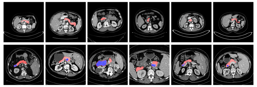
Figure 1: An illustration of normal pancreases on NIH dataset roth2015deeporgan and abnormal cystic pancreases on JHMI dataset zhou2017deep shown in the first and second row respectively. Normal pancreas regions are masked as red and abnormal pancreas regions are marked as blue. The pancreas usually occupies a small region in a whole CT scan. Best viewed in color.

An obstacle to train 3D deep segmentation networks is that it suffers from the “out of memory” problem. 2D FCNs can accept a whole 2D slice as input, but 3D FCNs cannot be fed a whole 3D volume due to the limited GPU memory size. A common solution is to train 3D FCNs from small sub-volumes and test them in a sliding-window manner milletari2016v bui20173d cciccek20163d chen2017voxresnet yu2017automatic , i.e., performing 3D segmentation on densely and uniformly sampled sub-volumes one by one. Usually, these neighboring sampled sub-volumes overlap with each other to improve the robustness of the final 3D results. It is worth noting that the overlap size is a trade-off between the segmentation accuracy and the time cost. Setting a larger/smaller overlap size generally leads to a better/worse segmentation accuracy but takes more/less time during testing.

To address these issues, we propose a concise and effective framework to train 3D deep networks for pancreas segmentation, which can simultaneously achieve high segmentation accuracy and low time cost. Our framework is formulated into a coarse-to-fine manner. In the training stage, we first train a 3D FCN from the sub-volumes sampled from an entire CT volume. We call this ResDSN Coarse model, which aims at obtaining the rough location of the target pancreas from the whole CT volume by making full use of the overall 3D context. Then, we train another 3D FCN from the sub-volumes sampled only from the ground truth bounding boxes of the target pancreas. We call this the ResDSN Fine model, which can refine the segmentation based on the coarse result. In the testing stage, we first apply the coarse model in the sliding-window manner to a whole CT volume to extract the most probable location of the pancreas. Since we only need a rough location for the target pancreas in this step, the overlap size is set to a small value. Afterwards, we apply the fine model in the sliding-window manner to the coarse pancreas region, but by setting a larger overlap size. Thus, we can efficiently obtain a fine segmentation result and we call the coarse-to-fine framework by ResDSN C2F.

Note that, the meaning of “coarse-to-fine” in our framework is twofold. First, it means the input region of interests (RoIs) for the ResDSN Coarse model and the ResDSN Fine model are different, i.e., a whole CT volume for the former one and a rough bounding box of the target pancreas for the latter one. We refer to this as coarse-to-fine RoIs, which is designed to achieve better segmentation performance. The coarse step removes a large amount of the unrelated background region, then with a relatively smaller region to be sampled as input, the fine step can much more easily learn cues which distinguish the pancreas from the local background, i.e., exploit local context which makes it easier to obtain a more accurate segmentation result. Second, it means the overlap sizes used for the ResDSN Coarse model and the ResDSN Fine model during inference are different, i.e., small and large overlap sizes for them, respectively. We refer to this as coarse-to-fine overlap sizes, which is designed for efficient 3D inference.

Recently, it is increasingly realized that deep networks are vulnerable to adversarial examples, i.e., inputs that are almost indistinguishable from natural data which are imperceptible to a human, but yet classified incorrectly by the network goodfellow2014explaining szegedy2013intriguing xie2017adversarial . This problem is even more serious for medical learning systems, as they may cause incorrect decisions, which could mislead human doctors. Adversarial examples may be only a small subset of the space of all medical images, so it is possible that they will only rarely occur in real datasets. But, even so, they could potentially have major errors. Analyzing them can help medical imaging researchers to understand more about their deep network based model, with the ultimate goal of increasing robustness. In this chapter, we generate 3D adversarial examples by the gradient-based methods goodfellow2014explaining ; kurakin2016scale and investigate the threat of these 3D adversarial examples on our framework. We also show how to defend against these adversarial examples.

The contributions of this chapter can be summarized into two aspects: (1) A novel 3D deep network based framework which leverages the rich spatial information for medical image segmentation, which achieves the state-of-the-art performance with relative low time cost on segmenting both normal and abnormal pancreases; (2) A systematic analysis about the threat of 3D adversarial examples on our framework as well as the adversarial defense methods.

The first part of this work appeared as a conference paper ZhuXSFY18 , in which Zhuotun Zhu, Yingda Xia, and Wei Shen made contributions to. The second part was contributed by Yingwei Li, Yuyin Zhou, and Wei Shen. Elliot K. Fishman and Alan L. Yuille oversaw the entire project. This chapter extends the previous work ZhuXSFY18 by including the analysis about the 3D adversarial attacks and defenses for our framework and more experimental results.·

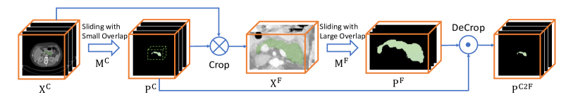
Figure 2: Flowchart of the proposed 3D coarse-to-fine segmentation system in the testing phase. We first apply “ResDSN Coarse” with a small overlapped sliding window to obtain a rough pancreas region and then use the “ResDSN Fine” model to refine the results with a large overlapped sliding window. Best viewed in color.

2 Related Work

2.1 Deep Learning based Medical Image Segmentation

The medical image analysis community is facing a revolution brought by the fast development of deep networks KrizhevskySH12 SimonyanZ14a . Deep Convolutional Neural Networks (CNNs) based methods have dominated the research area of volumetric medical image segmentation in the last few years. Generally speaking, CNN-based methods for volumetric medical image segmentation can be divided into two major categories: 2D CNNs based and 3D CNNs based.

2D CNNs for Medical Image Segmentation

2D CNNs based methods roth2015deeporgan roth2016spatial HavaeiDWBCBPJL17 MoeskopsWVGLVI17 ronneberger2015u WangZTSFY18 Yan-MultiOrgan18 performed volumetric segmentation slice by slice from different views, and then fused the 2D segmentation results to obtain a 3D Volumetric Segmentation result. In the early stage, the 2D segmentation based models were trained from image patches and tested in a patch by patch manner roth2015deeporgan , which is time consuming. Since the introduction of fully convolution networks (FCNs) LongSD15 , almost all the 2D segmentation methods are built upon 2D FCNs to perform holistic slice segmentation during both training and testing. Havaei et al HavaeiDWBCBPJL17 proposed a two-pathway FCN architecture, which exploited both local features as well as more global contextual features simultaneously by the two pathways. Roth et al roth2016spatial performed Pancreas segmentation by a holistic learning approach, which first segment pancreas regions by holistically-nested networks XieT15 and then refine them by the boundary maps obtained by robust spatial aggregation using random forest. The U-Net ronneberger2015u is one of the most popular FCN architectures for medical image segmentation, which is a encoder-decoder network, but with additional short connection between encoder and decoder paths. Based on the fact that a pancreas only takes up a small fraction of the whole scan, Zhou et al. zhou2017fixed proposed to find the rough pancreas region and then learn a FCN based fixed-point model to refine the pancreas region iteratively. Their method is also based on a coarse-to-fine framework, but it only considered coarse-to-fine RoIs. Besides coarse-to-fine RoIs, our coarse-to-fine method also takes coarse-to-fine overlap sizes into account, which is designed specifically for efficient 3D inference.

3D CNNs for Medical Image Segmentation

Although 2D CNNs based methods achieved considerable progress, they are not optimal for medical image segmentation, as they cannot make full use of the 3D context encoded in volumetric data. Several 3D CNNs based segmentation methods have been proposed. The 3D U-Net cciccek20163d extended the previous 2D U-Net architecture ronneberger2015u by replacing all 2D operations with their 3D counterparts. Based on the architecture of the 3D U-Net, the V-Net milletari2016v introduced residual structures he2016deep (short term skip connection) into each stage of the network. Chen et al chen2017voxresnet proposed a deep voxel-wise residual network for 3D brain segmentation. Both I2I-3D merkow2016dense and 3D-DSN dou20173d included auxiliary supervision via side outputs into their 3D deep networks. Despite the success of 3D CNNs as a technique for segmenting the target organs, such as prostate milletari2016v and kidney cciccek20163d , very few techniques have been developed for leveraging 3D spatial information on the challenging pancreas segmentation. Gibson et al. gibson2018automatic proposed the DenseVNet which is however constrained to have shallow encoders due to the computationally demanding dense connections. Roth et al. roth2018towards extended 3D U-Net to segment the pancreas, while obtaining good results, this method has the following shortcomings, 1) the input of their networks is fixed to $120\times 120\times 120$, which is very computationally demanding due to this large volume size, 2) the rough pancreas bounding box is resampled to a fixed size as their networks input, which loses information and flexibility, and cannot deal with the intrinsic large variations of pancreas in shape and size. Therefore, we propose our 3D coarse-to-fine framework that works on both normal and abnormal CT data to ensure both low computation cost and high pancreas segmentation accuracy.

2.2 Adversarial Attacks and Defenses for Medical Image Segmentation Networks

Deep learning has become increasingly adopted within the medical imaging community for a wide range of tasks including classification, segmentation, detection, etc. Though achieving tremendous success in various problems, CNNs have been demonstrated to be extremely vulnerable to adversarial examples, i.e., images which are crafted by human-imperceptible perturbations goodfellow2014explaining szegedy2013intriguing xie2017adversarial . Xie et al. xie2017adversarial were first to make adversarial examples for semantic segmentation, which is directly related to medical image segmentation. Paschali et.al. paschali2018generalizability used the code from Xie et al. xie2017adversarial and showed that state-of-the-art networks such as Inception szegedy2016rethinking and UNet Ronneberger_2015_UNet are still extremely susceptible to adversarial examples for skin lesion classification and whole brain segmentation. It was also demonstrated that adversarial examples are superior in pushing a network to its limits and evaluating its robustness in paschali2018generalizability . Additionally, Huang et.al. huang2018some pointed out that the robustness of deep learning-based reconstruction techniques for limited angle tomography remains a concern due to its vulnerability to adversarial examples. This makes the robustness of neural networks for clinical applications an important unresolved issue.

To alleviate such adversarial effects for clinical applications, we investigate the application of adversarial training szegedy2013intriguing for improving the robustness of deep learning algorithms in the medical area. Adversarial training was first proposed by Szegedy et.al. szegedy2013intriguing to increase robustness by augmenting training data with adversarial examples. Madry et.al. madry2017towards further validated that adversarially trained models can be robust against white-box attacks, i.e., with knowledge of the model parameters. Note that clinical applications of deep learning require a high level of safety and security huang2018some . Our experiments empirically demonstrate that adversarial training can be greatly beneficial for improving the robustness of 3D deep learning-based models against adversarial examples.

3 Method

3.1 A 3D Coarse-to-fine Framework for Medical Image Segmentation

In this section, we elaborate our 3D coarse-to-fine framework which includes a coarse stage and a fine stage afterwards. We first formulate a segmentation model that can be generalized to both coarse stage and fine stage. Later in Sec. 3.1 and Sec. 3.1, we will customize the segmentation model to these two stages, separately.

We denote a 3D CT-scan volume by $\mathbf{X}$. This is associated with a human-labeled per-voxel annotation $\mathbf{Y}$, where both $\mathbf{X}$ and $\mathbf{Y}$ have size $W\times H\times D$, which corresponds to axial, sagittal and coronal views, separately. The ground-truth segmentation mask $\mathbf{Y}$ has a binary value $y_{i}$, $i=1,\cdots,WHD$, at each spatial location $i$ where $y_{i}=1$ indicates that $x_{i}$ is a pancreas voxel. Denote a segmentation model by $\mathbb{M}:\mathbf{P}={\mathbf{f}\!\left(\mathbf{X};\boldsymbol{\Theta}\right)}$, where $\boldsymbol{\Theta}$ indicates model parameters and $\mathbf{P}$ means the binary prediction volume. Specifically in a neural network with $L$ layers and parameters $\boldsymbol{\Theta}=\{\mathcal{W},\mathcal{B}\}$, $\mathcal{W}$ is a set of weights and $\mathcal{B}$ is a set of biases, where $\mathcal{W}=\{\mathbf{W}^{1},\mathbf{W}^{2},\cdots,\mathbf{W}^{L}\}$ and $\mathcal{B}=\{\mathbf{B}^{1},\mathbf{B}^{2},\cdots,\mathbf{B}^{L}\}$. Given that $p(y_{i}|x_{i};\boldsymbol{\Theta})$ represents the predicted probability of a voxel $x_{i}$ being what is the labeled class at the final layer of the output, the negative log-likelihood loss can be formulated as:

$$\mathcal{L}=\mathcal{L}(\mathbf{X};\boldsymbol{\Theta})=-\sum_{x_{i}\in\mathbf{X}}{\log(p(y_{i}|x_{i};\boldsymbol{\Theta}))}.$$ (1)

It is also known as the cross entropy loss in our binary segmentation setting. By thresholding $p(y_{i}|x_{i};\boldsymbol{\Theta})$, we can obtain the binary segmentation mask $\mathbf{P}$.

We also add some auxiliary layers to the neural network, which produces side outputs under deep supervision lee2015deeply . These auxiliary layers form a branch network and facilitate feature learning at lower layer of the mainstream network. Each branch network shares the weights of the first $d$ layers from the mainstream network, which is denoted by $\boldsymbol{\Theta}_{d}=\{\mathcal{W}_{d},\mathcal{B}_{d}\}$ and has its own weights $\widehat{\boldsymbol{\Theta}}_{d}$ to output the per-voxel prediction. Similarly, the loss of an auxiliary network can be formulated as:

$$\mathcal{L}_{d}(\mathbf{X};\boldsymbol{\Theta}_{d},\widehat{\boldsymbol{\Theta}}_{d})=\sum_{x_{i}\in\mathbf{X}}{-\log(p(y_{i}|x_{i};\boldsymbol{\Theta}_{d},\widehat{\boldsymbol{\Theta}}_{d}))},$$ (2)

which is abbreviated as $\mathcal{L}_{d}$. Finally, stochastic gradient descent is applied to minimize the negative log-likelihood, which is given by following regularized objective function:

$$\mathcal{L}_{overall}=\mathcal{L}+\sum_{d\in\mathcal{D}}\xi_{d}\mathcal{L}_{d}+\lambda({\|\boldsymbol{\Theta}\|}^{2}+\sum_{d\in\mathcal{D}}{\|\widehat{\boldsymbol{\Theta}}_{d}\|)}^{2},$$ (3)

where $\mathcal{D}$ is a set of branch networks for auxiliary supervisions, $\xi_{d}$ balances the importance of each auxiliary network and $l_{2}$ regularization is added to the objective to prevent the networks from overfitting. For notational simplicity, we keep a segmentation model that is obtained from the overall function described in Eq. 3 denoted by $\mathbb{M}:\mathbf{P}={\mathbf{f}\!\left(\mathbf{X};\boldsymbol{\Theta}\right)}$, where $\boldsymbol{\Theta}$ includes parameters of the mainstream network and auxiliary networks.

Coarse Stage

In the coarse stage, the input of “ResDSN Coarse” is sampled from the whole CT-scan volume denoted by $\mathbf{X}^{\textrm{C}}$, on which the coarse segmentation model $\mathbb{M}^{\textrm{C}}:\mathbf{P}^{\textrm{C}}={\mathbf{f}^{\textrm{C}}\!\left(\mathbf{X}^{\textrm{C}};\boldsymbol{\Theta}^{\textrm{C}}\right)}$ is trained on. All the C superscripts depict the coarse stage. The goal of this stage is to efficiently produce a rough binary segmentation $\mathbf{P}^{\textrm{C}}$ from the complex background, which can get rid of regions that are segmented as non-pancreas with a high confidence to obtain an approximate pancreas volume. Based on this approximate pancreas volume, we can crop from the original input $\mathbf{X}^{\textrm{C}}$ with a rectangular cube derived from $\mathbf{P}^{\textrm{C}}$ to obtain a smaller 3D image space $\mathbf{X}^{\textrm{F}}$, which is surrounded by simplified and less variable context compared with $\mathbf{X}^{\textrm{C}}$. The mathematic definition of $\mathbf{X}^{\textrm{F}}$ is formulated as:

$$\mathbf{X}^{\textrm{F}}=\textrm{Crop}[\mathbf{X}^{\textrm{C}}\otimes\mathbf{P}^{\textrm{C}};\mathbf{P}^{\textrm{C}},m],$$ (4)

where $\otimes$ means an element-wise product. The function $\textrm{Crop}[\mathbf{X};\mathbf{P},m]$ denotes cropping $\mathbf{X}$ via a rectangular cube that covers all the $1$’s voxels of a binary volume $\mathbf{P}$ added by a padding margin $m$ along three axes. Given $\mathbf{P}$, the functional constraint imposed on $\mathbf{X}$ is that they have exactly the same dimensionality in 3D space. The padding parameter $m$ is empirically determined in experiments, where it is used to better segment the boundary voxels of pancreas during the fine stage. The Crop operation acts as a dimensionality reduction to facilitate the fine segmentation, which is crucial to cut down the consuming time of segmentation. It is well-worth noting that the 3D locations of the rectangular cube which specifies where to crop $\mathbf{X}^{\textrm{F}}$ from $\mathbf{X}^{\textrm{C}}$ is recorded to map the fine segmentation results back their positions in the full CT scan.

Fine Stage

In the fine stage, the input of the ConvNet is sampled from the cropped volume $\mathbf{X}^{\textrm{F}}$, on which we train the fine segmentation model $\mathbb{M}^{\textrm{F}}:\mathbf{P}^{\textrm{F}}={\mathbf{f}^{\textrm{F}}\!\left(\mathbf{X}^{\textrm{F}};\boldsymbol{\Theta}^{\textrm{F}}\right)}$, where the F superscripts indicate the fine stage. The goal of this stage is to refine the coarse segmentation results from previous stage. In practice, $\mathbf{P}^{\textrm{F}}$ has the same volumetric size of $\mathbf{X}^{\textrm{F}}$, which is smaller than the original size of $\mathbf{X}^{\textrm{C}}$.

Coarse-to-Fine Segmentation

Our segmentation task is to give a volumetric prediction on every voxel of $\mathbf{X}^{\textrm{C}}$, so we need to map the $\mathbf{P}^{\textrm{F}}$ back to exactly the same size of $\mathbf{X}^{\textrm{C}}$ given by:

$$\mathbf{P}^{\textrm{C2F}}=\textrm{DeCrop}[\mathbf{P}^{\textrm{F}}\odot\mathbf{P}^{\textrm{C}};\mathbf{X}^{\textrm{F}},\mathbf{X}^{\textrm{C}}],$$ (5)

where $\mathbf{P}^{\textrm{C2F}}$ denotes the final volumetric segmentation, and $\odot$ means an element-wise replacement, and DeCrop operation defined on $\mathbf{P}^{\textrm{F}},\mathbf{P}^{\textrm{C}},\mathbf{X}^{\textrm{F}}\textrm{ and }\mathbf{X}^{\textrm{C}}$ is to replace a pre-defined rectangular cube inside $\mathbf{P}^{\textrm{C}}$ by $\mathbf{P}^{\textrm{F}}$, where the replacement locations are given by the definition of cropping $\mathbf{X}^{\textrm{F}}$ from $\mathbf{X}^{\textrm{C}}$ given in Eq. 4.

All in all, our entire 3D-based coarse-to-fine segmentation framework during testing is illustrated in Fig 2.

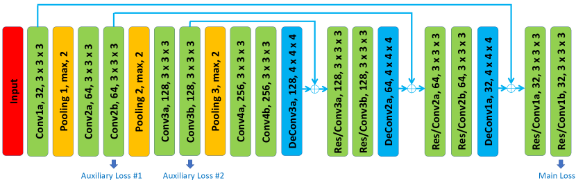
Figure 3: Illustration of our 3D convolutional neural network for volumetric segmentation. The encoder path is composed from “Conv1a” to “Conv4b” while the decoder path is from “DeConv3a” to “Res/Conv1b”. Each convolution or deconvolution layer consists of one convolution followed by a BatchNorm and a ReLU. To clarify, “Conv1a, 32, $3\times 3\times 3$” means the convolution operation with $32$ channels and a kernel size of $3\times 3\times 3$. “Pooling 1, max, $2$” means the max pooling operation with kernel size of $2\times 2\times 2$ and a stride of two. Long residual connections are illustrated by the blue concrete lines. Blocks with same color mean the same operations. Best viewed in color.

Network Architecture

As shown in Fig. 3, we provide an illustration of our convolutional network architecture. Inspired by V-Net milletari2016v , 3D U-Net cciccek20163d , and VoxResNet chen2017voxresnet , we have an encoder path followed by a decoder path each with four resolution steps. The left part of network acts as a feature extractor to learn higher and higher level of representations while the right part of network decompresses compact features into finer and finer resolution to predict the per-voxel segmentation. The padding and stride of each layer (Conv, Pooling, DeConv) are carefully designed to make sure the densely predicted output is the same size as the input.

The encoder sub-network on the left is divided into different steps that work on different resolutions. Each step consists of one to two convolutions, where each convolution is composed of $3\times 3\times 3$ convolution followed by a batch normalization (BN ioffe2015batch ) and a rectified linear unit (ReLU nair2010rectified ) to reach better convergence, and then a max pooling layer with a kernel size of $2\times 2\times 2$ and strides of two to reduce resolutions and learn more compact features. The downsampling operation implemented by max-pooling can reduce the size of the intermediate feature maps while increasing the size of the receptive fields. Having fewer size of activations makes it possible to double the number of channels during feature aggregation given the limited computational resource.

The decoder sub-network on the right is composed of several steps that operate on different resolutions as well. Each step has two convolutions with each one followed by a BatchNorm and a ReLU, and afterwards a Deconvolution with a kernel size of $4\times 4\times 4$ and strides of two is connected to expand the feature maps and finally predict the segmentation mask at the last layer. The upsampling operation that is carried out by deconvolution enlarges the resolution between each step, which increases the size of the intermediate activations so that we need to halve the number of channels due to the limited memory of the GPU card.

Apart from the left and right sub-networks, we impose a residual connection he2016deep to bridge short-cut connections of features between low-level layers and high-level layers. During the forward phase, the low-level cues extracted by networks are directly added to the high-level cues, which can help elaborate the fine-scaled segmentation, e.g., small parts close to the boundary which may be ignored during the feature aggregation due to the large size of receptive field at high-level layers. As for the backward phase, the supervision cues at high-level layers can be back-propagated through the short-cut way via the residual connections. This type of mechanism can prevent networks from gradient vanishing and exploding glorot2010understanding , which hampers network convergence during training.

We have one mainstream loss layer connected from “Res/Conv1b” and another two auxiliary loss layers connected from “Conv2b” and “Conv3b” to the ground truth label, respectively. For the mainstream loss in “Res/Conv1b” at the last layer which has the same size of data flow as one of the input, a $1\times 1\times 1$ convolution is followed to reduce the number of channels to the number of label classes which is $2$ in our case. As for the two auxiliary loss layers, deconvolution layers are connected to upsample feature maps to be the same as input.

The deep supervision imposed by auxiliary losses provides robustness to hyper-parameters choice, in that the low-level layers are guided by the direct segmentation loss, leading to faster convergence rate. Throughout this work, we have two auxiliary branches where the default parameters are $\xi_{1}=0.2$ and $\xi_{2}=0.4$ in Eq. 3 to control the importance of deep supervisions compared with the major supervision from the mainstream loss for all segmentation networks.

Method	Long Res	Short Res	Deep Super	Loss
ResDSN (Ours)	Sum	No	Yes	CE
FResDSN	Sum	Sum	Yes	CE
SResDSN	No	Sum	Yes	CE
3D U-Net cciccek20163d	Concat	No	No	CE
V-Net milletari2016v	Concat	Sum	No	DSC
VoxResNet chen2017voxresnet	No	Sum	Yes	CE
MixedResNet yu2017volumetric	Sum	Sum	Yes	CE
3D DSN dou20173d	No	No	Yes	CE
3D HED merkow2016dense	Concat	No	Yes	CE

Table 1: Configurations comparison of different 3D segmentation networks on medical image analysis. For all the abbreviated phrases, “Long Res” means long residual connection, “Short Res” means short residual connection, “Deep Super” means deep supervision implemented by auxiliary loss layers, “Concat” means concatenation, “DSC” means Dice-Sørensen Coefficient and “CE” means cross-entropy. For residual connection, it has two types: concatenation (“Concat”) or element-wise sum (“Sum”).

As shown in Table 1, we give the detailed comparisons of network configurations in terms of four aspects: long residual connection, short residual connection, deep supervision and loss function. Our backbone network architecture, named as “ResDSN”, is proposed with different strategies in terms of combinations of long residual connection and short residual connection compared with VoxResNet chen2017voxresnet , 3D HED merkow2016dense , 3D DSN dou20173d and MixedResNet yu2017volumetric . In this table, we also depict “FResDSN” and “SResDSN”, where “FResDSN” and “SResDSN” are similar to MixedResNet yu2017volumetric and VoxResNet chen2017voxresnet , respectively. As confirmed by our quantitative experiments in Sec. 4.1, instead of adding short residual connections to the network, e.g., “FResDSN” and “SResDSN”, we only choose the long residual element-wise sum, which can be more computationally efficient while even performing better than the “FResDSN” architecture which is equipped with both long and short residual connections. Moreover, ResDSN has noticeable differences with respect to the V-Net milletari2016v and 3D U-Net cciccek20163d . On the one hand, compared with 3D U-Net and V-Net which concatenate the lower-level local features to higher-level global features, we adopt the element-wise sum between these features, which outputs less number of channels for efficient computation. On the other hand, we introduce deep supervision via auxiliary losses into the network to yield better convergence.

3.2 3D Adversarial Examples

In this section, we discuss how to generate 3D adversarial examples for our segmentation framework as well as the defense method. We follow the notations defined in Sec. 3.1, i.e., $\mathbf{X}$ denotes a 3D CT-scan volume, $\mathbf{Y}^{\text{true}}$ denotes the corresponding ground-truth label, and $\mathcal{L}(\mathbf{X};\bm{\Theta})$ denotes the network loss function. To generate the adversarial example, the goal is to maximize the loss $\mathcal{L}(\mathbf{X}+\mathbf{r};\bm{\Theta})$ for the image $\mathbf{X}$, under the constraint that the generated adversarial example $\mathbf{X}^{\text{adv}}=\mathbf{X}+\mathbf{r}$ should look visually similar to the original image $\mathbf{X}$ and the corresponding predicted label $\mathbf{Y}^{\text{adv}}\neq\mathbf{Y}^{\text{true}}$. By imposing additional constraints such as $||\mathbf{r}||_{\infty}\leq\epsilon$, we can restrict the perturbation to be small enough to be imperceptible to humans.

Attack Methods

As for 3D adversarial attacking, we mainly adopt the gradient-based methods. They are

• Fast Gradient Sign Method (FGSM): FGSM goodfellow2014explaining is the first member in this attack family, which finds the adversarial perturbations in the direction of the loss gradient $\nabla_{\mathbf{X}}\mathcal{L}(\mathbf{X};\bm{\Theta})$. The update equation is

  $$\mathbf{X}^{\text{adv}}=\mathbf{X}+\epsilon\cdot\text{sign}(\nabla_{\mathbf{X}}\mathcal{L}(\mathbf{X};\bm{\Theta})).$$ (6)

• Iterative Fast Gradient Sign Method (I-FGSM): An extended iterative version of FGSM kurakin2016scale , which can be expressed as

  $$\mathbf{X}_{0}^{\text{adv}}=\mathbf{X}$$ (7)

  $$\mathbf{X}_{n+1}^{\text{adv}}=\text{Clip}_{\mathbf{X}}^{\epsilon}\left\{\mathbf{X}_{n}^{\text{adv}}+\alpha\cdot\text{sign}(\nabla_{\mathbf{X}}\mathcal{L}(\mathbf{X}_{n}^{adv};\bm{\Theta}))\right\},$$

  where $\text{Clip}_{\mathbf{X}}^{\epsilon}$ indicates the resulting images are clipped within the $\epsilon$-ball of the original image $\mathbf{X}$, $n$ is the iteration number and $\alpha$ is the step size.

Defending against 3D adversarial examples

Following madry2017towards , defending against adversarial examples can be expressed as a saddle point problem, which comprises of an inner maximization problem and an outer minimization problem. More precisely, our objective for defending against 3D adversarial examples is formulated as following:

$$\min_{\mathbf{\Theta}}\rho(\bm{\Theta}),\quad\text{ where }\quad\rho(\bm{\Theta})=\mathbb{E}_{(\mathbf{X})\sim\mathcal{D}}\left[\max_{\mathbf{r}\in\mathcal{S}}\mathcal{L}(\mathbf{X}+\mathbf{r};\bm{\Theta})\right].$$ (8)

$\mathcal{S}$ and $\mathcal{D}$ denote the set of allowed perturbations and the data distribution, respectively.

4 Experiments

In this section, we demonstrate our experimental results, which consists of two parts. In the first part, we show the performance of our framework on pancreas segmentation. We first describe in detail how we conduct training and testing on the coarse and fine stages, respectively. Then we give the comparison results on three pancreas datasets: the NIH pancreas dataset roth2015deeporgan , the JHMI pathological cyst dataset zhou2017deep and the JHMI pancreas dataset. In the second part, we discuss the adversarial attack and defense results on our framework.

4.1 Pancreas Segmentation

Network Training and Testing

All our experiments were run on a desktop equipped with the NVIDIA TITAN X (Pascal) GPU and deep neural networks were implemented based on the CAFFE jia2014caffe platform customized to support 3D operations for all necessary layers, e.g., “convolution”, “deconvolution” and “pooling”, etc. For the data pre-processing, we simply truncated the raw intensity values to be in $[-100,240]$ and then normalized each raw CT case to have zero mean and unit variance to decrease the data variance caused by the physical processes gravel2004method of medical images. As for the data augmentation in the training phase, unlike sophisticated processing used by others, e.g., elastic deformation milletari2016v ronneberger2015u , we utilized simple but effective augmentations on all training patches, i.e., rotation ($90\degree,180\degree,\textrm{ and }270\degree$) and flip in all three axes (axial, sagittal and coronal), to increase the number of 3D training samples which can alleviate the scarce of CT scans with expensive human annotations. Note that different CT cases have different physical resolutions, but we keep their resolutions unchanged. The input size of all our networks is denoted by $W_{I}\times H_{I}\times D_{I}$, where $W_{I}=H_{I}=D_{I}=64$.

For the coarse stage, we randomly sampled $64\times 64\times 64$ sub-volumes from the whole CT scan in the training phase. In this case, a sub-volume can either cover a portion of pancreas voxels or be cropped from regions with non-pancreas voxels at all, which acts as a hard negative mining to reduce the false positive. In the testing phase, a sliding window was carried out to the whole CT volume with a coarse stepsize that has small overlaps within each neighboring sub-volume. Specifically, for a testing volume with a size of $W\times H\times D$, we have a total number of $(\lfloor\frac{W}{W_{I}}\rfloor+n)\times(\lfloor\frac{H}{H_{I}}\rfloor+n)\times(\lfloor\frac{D}{D_{I}}\rfloor+n)$ sub-volumes to be fed into the network and then combined to obtain the final prediction, where $n$ is a parameter to control the sliding overlaps that a larger $n$ results in a larger overlap and vice versa. In the coarse stage for the low time cost concern, we set $n=6$ to efficiently locate the rough region of pancreas $\mathbf{X}^{\textrm{F}}$ defined in Eq. 4 from the whole CT scan $\mathbf{X}^{\textrm{C}}$.

For the fine stage, we randomly cropped $64\times 64\times 64$ sub-volumes constrained to be from the pancreas regions defined by ground-truth labels during training. In this case, a training sub-volume was assured to cover pancreatic voxels, which was specifically designed to be capable of segmentation refinement. In the testing phase, we only applied the sliding window on $\mathbf{X}^{\textrm{F}}$ with a size of $W_{F}\times H_{F}\times D_{F}$. The total number of sub-volumes to be tested is $(\lfloor\frac{W_{F}}{W_{I}}\rfloor+n)\times(\lfloor\frac{H_{F}}{H_{I}}\rfloor+n)\times(\lfloor\frac{D_{F}}{D_{I}}\rfloor+n)$. In the fine stage for the high accuracy performance concern, we set $n=12$ to accurately estimate the pancreatic mask $\mathbf{P}^{\textrm{F}}$ from the rough segmentation volume $\mathbf{X}^{\textrm{F}}$. In the end, we mapped the $\mathbf{P}^{\textrm{F}}$ back to $\mathbf{P}^{\textrm{C}}$ to obtain $\mathbf{P}^{\textrm{C2F}}$ for the final pancreas segmentation as given in Eq. 5, where the mapping location is given by the cropped location of $\mathbf{X}^{\textrm{F}}$ from $\mathbf{X}^{\textrm{C}}$.

After we get the final binary segmentation mask, we denote $\mathcal{P}$ and $\mathcal{Y}$ to be the set of pancreas voxels in the prediction and ground truth, separately, i.e., $\mathcal{P}=\{i|p_{i}=1\}$ and $\mathcal{Y}=\{i|y_{i}=1\}$. The evaluation metric is defined by the Dice-Sørensen Coefficient (DSC) formulated as $\text{DSC}(\mathcal{P},\mathcal{Y})=\frac{2\times|\mathcal{P}\cap\mathcal{Y}|}{|\mathcal{P}|+|\mathcal{Y}|}$. This evaluation measurement ranges in $[0,1]$ where $1$ means a perfect prediction.

NIH Pancreas Dataset

We conduct experiments on the NIH pancreas segmentation dataset roth2015deeporgan , which contains $82$ contrast-enhanced abdominal CT volumes provided by an experienced radiologist. The size of CT volumes is $512\times 512\times D$, where $D\in[181,466]$ and their spatial resolutions are $w\times h\times d$, where $d=1.0\textrm{mm}$ and $w=h$ that ranges from $0.5\textrm{mm}$ to $1.0\textrm{mm}$. Data pre-processing and data augmentation were described in Sec. 4.1. Note that we did not normalize the spatial resolution into the same one since we wanted to impose the networks to learn to deal with the variations between different volumetric cases. Following the training protocol roth2015deeporgan , we perform $4$-fold cross-validation in a random split from $82$ patients for training and testing folds, where each testing fold has $21,21,20$ and $20$ cases, respectively. We trained networks illustrated in Fig. 3 by SGD optimizer with a $16$ mini-batch, a $0.9$ momentum, a base learning rate to be $0.01$ via polynomial decay (the power is $0.9$) in a total of $80\rm{,}000$ iterations, and the weight decay $0.0005$. Both training networks in the coarse and fine stages shared the same training parameter settings except that they took a $64\times 64\times 64$ input sampled from different underlying distributions described in Sec. 4.1, which included the details of testing settings as well. We average the score map of overlapped regions from the sliding window and throw away small isolated predictions whose portions are smaller than $0.2$ of the total prediction, which can remove small false positives. For DSC evaluation, we report the average with standard deviation, max and min statistics over all $82$ testing cases as shown in Table 2.

Method	Mean DSC	Max DSC	Min DSC
ResDSN C2F (Ours)	$\bm{84.59\pm{4.86}}\%$	$\bm{91.45}\%$	$\bm{69.62}\%$
ResDSN Coarse (Ours)	$83.18\pm{6.02}\%$	$91.33\%$	$58.44\%$
Cai et al. cai2017improving	$82.4\pm{6.7}\%$	$90.1\%$	$60.0\%$
Zhou et al. zhou2017fixed	$82.37\pm{5.68}\%$	$90.85\%$	$62.43\%$
Dou et al. dou20173d	$82.25\pm{5.91}\%$	$90.32\%$	$62.53\%$
Roth et al. roth2016spatial	$78.01\pm{8.20}\%$	$88.65\%$	$34.11\%$
Yu et al. yu2017automatic	$71.96\pm{15.34}\%$	$89.27\%$	$0\%$

Table 2: Evaluation of different methods on the NIH dataset. Our proposed framework achieves state-of-the-art by a large margin compared with previous state-of-the-arts.

First of all, our overall coarse-to-fine framework outperforms previous state-of-the-art by nearly $2.2\%$ (Cai et al. cai2017improving and Zhou et al. zhou2017fixed ) in terms of average DSC, which is a large improvement. The lower standard deviation of DSC shows that our method is the most stable and robust across all different CT cases. Although the enhancement of max DSC of our framework is small due to saturation, the improvement of the min DSC over the second best (Dou et al. dou20173d ) is from $62.53\%$ to $69.62\%$, which is a more than $7\%$ advancement. The worst case almost reaches $70\%$, which is a reasonable and acceptable segmentation result. After coarse-to-fine, the segmentation result of the worst case is improved by more than $11\%$ after the 3D-based refinement from the 3D-based coarse result. The overall average DSC was also improved by $1.41\%$, which proves the effectiveness of our framework.

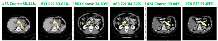
Figure 4: Examples of segmentation results reported by “ResDSN Coarse” and “ResDSN C2F” on a same slice in the axial view from NIH case $\#33$, $\#63$ and $\#74$, respectively. Numbers after “Coarse” or “C2F” mean testing DSC. Red, green and yellow indicate the ground truth, prediction and overlapped regions, respectively. Best viewed in color.

As shown in Fig 4, we report the segmentation results by “ResDSN Coarse” and “ResDSN C2F” on the same slice for comparison. Note that yellow regions are the correctly predicted pancreas. For the NIH case $\#33$, which is the min DSC case reported by both “ResDSN Coarse” and “ResDSN C2F”, the “ResDSN C2F” successfully predict more correct pancreas regions at the bottom, which is obviously missed by “ResDSN Coarse”. If the coarse segmentation is bad, e.g., case $\#33$ and $\#63$, our 3D coarse-to-fine can significantly improve the segmentation results by as much as $10\%$ in DSC. However, if the coarse segmentation is already very good, e.g., case $\#74$, our proposed method cannot improve too much. We conclude that our proposed “ResDSN C2F” shows its advancement over 2D methods by aggregating rich spatial information and is more powerful than other 3D methods on the challenging pancreas segmentation task.

JHMI Pathological Cyst Dataset

We verified our proposed idea on the JHMI pathological cyst dataset zhou2017deep of abdominal CT scans as well. Different from the NIH pancreas dataset, which only contains healthy pancreas, this dataset includes pathological cysts where some can be or can become cancerous. The pancreatic cancer stage largely influences the morphology of the pancreas lasboo2010morphological that makes this dataset extremely challenging for considering the large variants.

This dataset has a total number of $131$ contrast-enhanced abdominal CT volumes with human-labeled pancreas annotations. The size of CT volumes is $512\times 512\times D$, where $D\in[358,1121]$ that spans a wider variety of thickness than one of the NIH dataset. Following the training protocol zhou2017deep , we conducted $4$-fold cross validation on this dataset where each testing fold has $33,33,32$ and $33$ cases, respectively. We trained networks illustrated in Fig. 3 in both the coarse and fine stage with the same training settings as on the NIH except that we trained a total of $300\rm{,}000$ iterations on this pathological dataset since a pancreas with cysts is more difficult to segment than a normal case. In the testing phase, we vote the prediction map of overlapped regions from the sliding window and ignore small isolated pancreas predictions whose portions are smaller than $0.05$ of the total prediction. As shown in Table. 3, we compare our framework with only one available published results on this dataset. “ResDSN C2F” achieves an average ${80.56\%}$ DSC that consistently outperforms the 2D based coarse-to-fine method zhou2017deep , which confirms the advantage of leveraging the rich spatial information along three axes. What’s more, the “ResDSN C2F” improves the “ResDSN Coarse” by ${2.60\%}$ in terms of the mean DSC, which is a remarkable improvement that proves the effectiveness of the proposed 3D coarse-to-fine framework. Both  zhou2017deep and our method have multiple failure cases whose testing DSC are $0$, which indicates the segmentation of pathological organs is a more tough task. Due to these failure cases, we observe a large deviation on this pathological pancreas dataset compared with results on the NIH healthy pancreas dataset.

Method	Mean DSC
ResDSN C2F (Ours)	$\bm{80.56\pm{13.36}}\%$
ResDSN Coarse (Ours)	$77.96\pm{13.36}\%$
Zhou et al. zhou2017deep	$79.23\pm{9.72}\%$

Table 3: Evaluations on the JHMI pathological pancreas.

JHMI Pancreas Dataset

In order to further validate the superiority of our 3D model, We also evaluate our approach on a large high-quality dataset collected by the radiologists in our team. This dataset contains $305$ contrast-enhanced abdominal CT volumes, and each of them is manually labeled with pancreas masks. Each CT volume consists of $319\sim 1051$ slices of $512\times 512$ pixels, and have voxel spatial resolution of $([0.523\sim 0.977]\times[0.523\sim 0.977]\times 0.5)\textup{mm}^{3}$. Following the training protocol roth2015deeporgan , we perform $4$-fold cross-validation in a random split from all patients for training and testing folds, where each testing fold has $77,76,76$ and $76$ cases, respectively. We demonstrate the superiority of our 3D model by comparing with the 2D baseline zhou2017fixed (see Table 4).

Method	Mean DSC	Max DSC	Min DSC
ResDSN Coarse (Ours)	$\bm{87.84\pm{7.27}}\%$	$\bm{95.27}\%$	$0.07\%$
Zhou et al. zhou2017deep	$84.99\pm{7.42}\%$	$93.45\%$	$\bm{3.76}\%$

Table 4: Evaluations on the JHMI pancreas dataset.

Ablation Study

In this section, we conduct the ablation studies about residual connection, time efficiency and deep supervision to further investigate the effectiveness and efficiency of our proposed framework for pancreas segmentation.

Residual Connection

We discuss how different combinations of residual connections contribute to the pancreas segmentation task on the NIH dataset. All the residual connections are implemented in the element-wise sum and they shared exactly the same deep supervision connections, cross-validation splits, data input, training and testing settings except that the residual structure is different from each other. As given in Table. 5, we compare four configurations of residual connections of 3D based networks only in the coarse stage. The major differences between our backbone network “ResDSN” with respect to “FResDSN”, “SResDSN” and “DSN” are depicted in Table. 1. “ResDSN” outperforms other network architectures in terms of average DSC and a small standard deviation even through the network is not as sophisticated as “FResDSN”, which is the reason we adopt “ResDSN” for efficiency concerns in the coarse stage.

Method	Mean DSC	Max DSC	Min DSC
ResDSN Coarse (Ours)	$\bm{83.18\pm{6.02}}\%$	$91.33\%$	$58.44\%$
FResDSN Coarse	$83.11\pm{6.53}\%$	$91.34\%$	$61.97\%$
SResDSN Coarse	$82.82\pm{5.97}\%$	$90.33\%$	$62.43\%$
DSN dou20173d Coarse	$82.25\pm{5.91}\%$	$90.32\%$	$62.53\%$

Table 5: Evaluation of different residual connections on NIH.

Time Efficiency

We discuss the time efficiency of the proposed coarse-to-fine framework with a smaller overlap in the coarse stage for the low consuming time concern while a larger one in the fine stage for the high prediction accuracy concern. The overlap size depends on how large we choose $n$ defined in Sec 4.1. We choose $n=6$ during the coarse stage while $n=12$ during the fine stage. Experimental results are shown in Table 6. “ResDSN Coarse” is the most efficient while the accuracy is the worst among three methods, which makes sense that we care more of the efficiency to obtain a rough pancreas segmentation. “ResDSN Fine” is to use a large overlap on an entire CT scan to do the segmentation which is the most time-consuming. In our coarse-to-fine framework, we combine the two advantages together to propose “ResDSN C2F” which can achieve the best segmentation results while the average testing time cost for each case is reduced by $36\%$ from $382$s to $245$s compared with “ResDSN Fine”. In comparison, it takes an experienced board certified Abdominal Radiologist 20 mins for one case, which verifies the clinical use of our framework.

Method	Mean DSC	$n$	Testing Time (s)
ResDSN C2F (Ours)	$\bm{84.59\pm{4.86}}\%$	$6\&12$	$245$
ResDSN Coarse (Ours)	$83.18\pm{6.02}\%$	$6$	$\bm{111}$
ResDSN Fine (Ours)	$83.96\pm{5.65}\%$	$12$	$382$

Table 6: Average time cost in the testing phase, where $n$ controls the overlap size of sliding windows during the inference.

Deep Supervision

We discuss how effective of the auxiliary losses to demonstrate the impact of the deep supervision on our 3D coarse-to-fine framework. Basically, we train our mainstream networks without any auxiliary losses for both coarse and fine stages, denoted as “Res C2F”, while keeping all other settings as the same, e.g., cross-validation splits, data pre-processing and post-processing. As shown in Table 7, “ResDSN C2F” outperforms “Res C2F” by $17.79\%$ to a large extent on min DSC and $0.53\%$ better on average DSC though it’s a little bit worse on max DSC. We conclude that 3D coarse-to-fine with deep supervisions performs better and especially more stable on the pancreas segmentation.

Method	Mean DSC	Max DSC	Min DSC
ResDSN C2F (Ours)	$\bm{84.59\pm{4.86}}\%$	$91.45\%$	$\bm{69.62}\%$
Res C2F	$84.06\pm{6.51}\%$	$\bm{91.72}\%$	$51.83\%$

Table 7: Ablation study of the deep supervision on NIH.

4.2 Adversarial Attack and Defense

In spite of the success of 3D learning models such as our proposed ResDSN, the robustness of neural networks for clinical applications remains a concern. In this section, we first show that our well-trained 3D model can be easily led to failure under imperceptible adversarial perturbations (see Sec. 4.2), and then investigate how to improve the adversarial robustness by employing adversarial training (see Sec. 4.2). We evaluate our approach by performing standard $4$-fold cross-validation on the JHMI pancreas dataset since this dataset is the largest in scale and has the best quality (see Sec. 4.1).

Robustness Evaluation

To evaluate the robustness of our well-trained 3D model, we attack the ResDSN Coarse model following the methods in Sec. 3.2. For both attacking methods, i.e., FGSM and I-FGSM, we set $\epsilon=0.03\Lambda$ so that the maximum perturbation can be small enough compared with the range of the truncated intensity value ($\Lambda$). Specially in the case of I-FGSM, the total iteration number $N$ and the step size $\alpha$ are set to be $5$ and $0.01\Lambda$, respectively. Following the test strategy in the coarse stage, we first compute the loss gradients of the $64\times 64\times 64$ sub-volumes obtained by a sliding window policy, and these gradients are then combined to calculate the final loss gradient map $\nabla_{\mathbf{X}}\mathcal{L}(\mathbf{X};\bm{\Theta})$ of each whole CT volume. The combine approach is also similar as the testing method described in Sec. 4.1, i.e., taking the average of loss gradient if a voxel is in the overlapped region. According to Eq. 6 and Eq. 7, the overall loss gradient can be used to generate adversarial examples which can then attack the 3D model for the purpose of robustness evaluation.

Attack Methods	Clean	FGSM goodfellow2014explaining	I-FGSM kurakin2016scale	Drop
ResDSN Coarse	$\bm{87.84\pm{7.27}}\%$	$42.68\%$	$2.01\%$	$85.83\%$
Adversarially-trained ResDSN Coarse	$79.09\pm{12.10}\%$	$\bm{67.58}\%$	$\bm{65.98}\%$	$\bm{13.11}\%$

Table 8: Comparative evaluation of the 3D segmentation model on clean (indicated by “Clean” in the table) and adversarial examples. Different attack methods,i.e., FGSM and I-FGSM, are used for generating the adversarial examples. We report the average accuracy and Dice overlap score along with the $\%$ maximum drop in performance on adversarial examples with respect to performance on clean data.

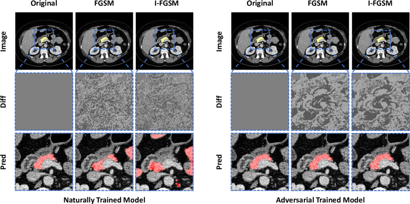
Figure 5: Qualitative comparison of adversarial examples and their effects on model predictions. Note that the added perturbation is effectively imperceptible to the human eye, and the difference between the original image and the adversarial image has been magnified by 5x(values shifted by 128) for a better visualization. Contrasting with prediction on original images, the crafted examples are able to successfully fool the models into generating incorrect segmentation maps. Meanwhile adversarial training can effectively alleviate such negative influence of adversarial attacks, hence improving the performance to a reasonable level. Image differences and predictions are zoomed in from the axial view to better visualize the finer details.

Defending Against Adversarial Attacks

To improve the adversarial robustness of our 3D segmentation model, we apply the adversarial training policy as described in Sec. 3.2. During each training iteration, $\mathbf{X_{adv}}$ is first randomly sampled in the $\epsilon\text{-ball}$ and then updated by I-FGSM so that $\mathcal{L}(\mathbf{X_{adv}};\bm{\Theta})$ can be maximized. Afterwards $\mathbf{X_{adv}}$ is fed to the model instead of $\mathbf{X}$ to update the parameter $\mathbf{\Theta}$. Note that we set the same maximum perturbation $\epsilon$, iteration number $N$ and step size $\alpha$ as in Sec. 4.2. Similar to the training process described in Sec. 4.1, our model is trained by SGD optimizer with a $128$ mini-batch, a $0.9$ momentum, a base learning rate to be $0.08$ via polynomial decay (the power is $0.9$) in a total of $10,000$ iterations, and the weight decay $0.0005$.

Results and Discussion

All attack and defense results are summarized in Table 8. We can see that both attack methods, i.e. FGSM and I-FGSM, can successfully fool the well-trained 3D ResDSN into producing incorrect prediction maps. More specifically, the dramatic performance drop of I-FGSM, i.e.,$85.83\%$ (from $87.84\%$ to $2.01\%$), suggests low adversarial robustness of the original model. Meanwhile the maximum performance drop decreases from $85.83\%$ to $13.11\%$, indicating that our adversarially-trained model can largely alleviate the adversarial effect and hence improving the robustness of our 3D model. Note that our baseline with “Clean” training has $87.84\%$ accuracy when tested on clean images, whereas its counterpart with adversarial training obtains $79.09\%$. This tradeoff between adversarial and clean training has been previously observed in tsipras2018robustness . We hope this tradeoff can be better studied in future research.

We also show a qualitative example in Fig. 5. As can be observed from the illustration, adversarial attacks to naturally trained 3D ResDSN induces many false positives, which makes the corresponding outcomes noisy. On the contrary, the adversarially trained 3D model yields similar performances even after applying I-FGSM. More specifically, the original average Dice score of 3D ResDSN is $89.30\%$, and after applying adversarial attack the performance drops to $48.45\%$ and $6.06\%$ with FGSM and I-FGSM respectively. However, when applying the same attack methods to the adversarial trained model, the performance only drops from $86.41\%$ to $80.32\%$ and $79.56\%$ respectively. In other words, employing adversarial training decreases the performance drop from $83.24\%$ to only $6.85\%$. This promising result clearly indicates that our adverarially-trained model can largely improve the adversarial robustness.

5 Conclusion

In this chapter, we proposed a novel 3D network called “ResDSN” integrated with a coarse-to-fine framework to simultaneously achieve high segmentation accuracy and low time cost. The backbone network “ResDSN” is carefully designed to only have long residual connections for efficient inference. In addition, we also analyzed the threat of adversarial attacks on our framework and showed how to improve the robustness against the attack. Experimental evidence indicates that our adversarially trained model can largely improve adversarial robustness than naturally trained ones.

To our best knowledge, the proposed 3D coarse-to-fine framework is one of the first works to segment the challenging pancreas using 3D networks which leverage the rich spatial information to achieve the state-of-the-art. We can naturally apply the proposed idea to other small organs, e.g., spleen, duodenum and gallbladder, etc, In the future, we will target on error causes that lead to inaccurate segmentation to make our framework more stable, and extend our 3D coarse-to-fine framework to cyst segmentation which can cause cancerous tumors, and the very important tumor segmentation zhu2018multi task.

References

- (1) Bui, T.D., Shin, J., Moon, T.: 3D densely convolution networks for volumetric segmentation. arXiv:1709.03199 (2017)
- (2) Cai, J., Lu, L., Xie, Y., Xing, F., Yang, L.: Improving deep pancreas segmentation in CT and MRI images via recurrent neural contextual learning and direct loss function (2017)
- (3) Chen, H., Dou, Q., Yu, L., Qin, J., Heng, P.A.: Voxresnet: Deep voxelwise residual networks for brain segmentation from 3D MR images. NeuroImage (2017)
- (4) Chen, L.C., Papandreou, G., Kokkinos, I., Murphy, K., Yuille, A.L.: Deeplab: Semantic image segmentation with deep convolutional nets, atrous convolution, and fully connected crfs. arXiv:1606.00915 (2016)
- (5) Çiçek, Ö., Abdulkadir, A., Lienkamp, S.S., Brox, T., Ronneberger, O.: 3D u-net: learning dense volumetric segmentation from sparse annotation. In: MICCAI (2016)
- (6) Dou, Q., Yu, L., Chen, H., Jin, Y., Yang, X., Qin, J., Heng, P.A.: 3D deeply supervised network for automated segmentation of volumetric medical images. MIA 41, 40–54 (2017)
- (7) Fang, Y., Xie, J., Dai, G., Wang, M., Zhu, F., Xu, T., Wong, E.: 3D deep shape descriptor. In: CVPR (2015)
- (8) Gibson, E., Giganti, F., Hu, Y., Bonmati, E., Bandula, S., Gurusamy, K., Davidson, B., Pereira, S.P., Clarkson, M.J., Barratt, D.C.: Automatic multi-organ segmentation on abdominal ct with dense v-networks. TMI (2018)
- (9) Glorot, X., Bengio, Y.: Understanding the difficulty of training deep feedforward neural networks. In: AISTATS (2010)
- (10) Goodfellow, I.J., Shlens, J., Szegedy, C.: Explaining and harnessing adversarial examples. In: ICLR (2015)
- (11) Gravel, P., Beaudoin, G., De Guise, J.A.: A method for modeling noise in medical images. TMI 23(10), 1221–1232 (2004)
- (12) Havaei, M., Davy, A., Warde-Farley, D., Biard, A., Courville, A.C., Bengio, Y., Pal, C., Jodoin, P., Larochelle, H.: Brain tumor segmentation with deep neural networks. MIA 35, 18–31 (2017)
- (13) He, K., Zhang, X., Ren, S., Sun, J.: Deep residual learning for image recognition. In: CVPR (2016)
- (14) Huang, Y., Würfl, T., Breininger, K., Liu, L., Lauritsch, G., Maier, A.: Some investigations on robustness of deep learning in limited angle tomography. In: MICCAI (2018)
- (15) Ioffe, S., Szegedy, C.: Batch normalization: Accelerating deep network training by reducing internal covariate shift. In: ICML (2015)
- (16) Jia, Y., Shelhamer, E., Donahue, J., Karayev, S., Long, J., Girshick, R., Guadarrama, S., Darrell, T.: CAFFE: Convolutional Architecture for Fast Feature Embedding. MM (2014)
- (17) Krizhevsky, A., Sutskever, I., Hinton, G.E.: Imagenet classification with deep convolutional neural networks. In: NIPS (2012)
- (18) Kurakin, A., Goodfellow, I., Bengio, S.: Adversarial machine learning at scale. In: ICLR (2017)
- (19) Lasboo, A.A., Rezai, P., Yaghmai, V.: Morphological analysis of pancreatic cystic masses. Academic radiology 17(3), 348–351 (2010)
- (20) Lee, C.Y., Xie, S., Gallagher, P., Zhang, Z., Tu, Z.: Deeply-supervised nets. In: AISTATS (2015)
- (21) Long, J., Shelhamer, E., Darrell, T.: Fully convolutional networks for semantic segmentation. In: CVPR (2015)
- (22) Madry, A., Makelov, A., Schmidt, L., Tsipras, D., Vladu, A.: Towards deep learning models resistant to adversarial attacks. In: ICLR (2018)
- (23) Merkow, J., Marsden, A., Kriegman, D., Tu, Z.: Dense volume-to-volume vascular boundary detection. In: MICCAI (2016)
- (24) Milletari, F., Navab, N., Ahmadi, S.A.: V-net: Fully convolutional neural networks for volumetric medical image segmentation. In: 3DV (2016)
- (25) Moeskops, P., Wolterink, J.M., van der Velden, B.H.M., Gilhuijs, K.G.A., Leiner, T., Viergever, M.A., Isgum, I.: Deep learning for multi-task medical image segmentation in multiple modalities. CoRR abs/1704.03379 (2017)
- (26) Nair, V., Hinton, G.E.: Rectified linear units improve restricted boltzmann machines. In: ICML (2010)
- (27) Paschali, M., Conjeti, S., Navarro, F., Navab, N.: Generalizability vs. robustness: Adversarial examples for medical imaging. In: MICCAI (2018)
- (28) Ronneberger, O., Fischer, P., Brox, T.: U-Net: Convolutional Networks for Biomedical Image Segmentation. International Conference on Medical Image Computing and Computer-Assisted Intervention (2015)
- (29) Ronneberger, O., Fischer, P., Brox, T.: U-net: Convolutional networks for biomedical image segmentation. In: MICCAI (2015)
- (30) Roth, H., Oda, M., Shimizu, N., Oda, H., Hayashi, Y., Kitasaka, T., Fujiwara, M., Misawa, K., Mori, K.: Towards dense volumetric pancreas segmentation in CT using 3D fully convolutional networks. In: SPIE (2018)
- (31) Roth, H.R., Lu, L., Farag, A., Shin, H.C., Liu, J., Turkbey, E.B., Summers, R.M.: Deeporgan: Multi-level deep convolutional networks for automated pancreas segmentation. In: MICCAI (2015)
- (32) Roth, H.R., Lu, L., Farag, A., Sohn, A., Summers, R.M.: Spatial aggregation of holistically-nested networks for automated pancreas segmentation. In: MICCAI (2016)
- (33) Shen, W., Wang, B., Jiang, Y., Wang, Y., Yuille, A.L.: Multi-stage multi-recursive-input fully convolutional networks for neuronal boundary detection. In: ICCV. pp. 2410–2419 (2017)
- (34) Shen, W., Wang, X., Wang, Y., Bai, X., Zhang, Z.: Deepcontour: A deep convolutional feature learned by positive-sharing loss for contour detection. In: CVPR (2015)
- (35) Simonyan, K., Zisserman, A.: Very deep convolutional networks for large-scale image recognition. arXiv:1409.1556 (2014)
- (36) Szegedy, C., Vanhoucke, V., Ioffe, S., Shlens, J., Wojna, Z.: Rethinking the inception architecture for computer vision. In: CVPR (2016)
- (37) Szegedy, C., Zaremba, W., Sutskever, I., Bruna, J., Erhan, D., Goodfellow, I., Fergus, R.: Intriguing properties of neural networks. In: ICLR (2014)
- (38) Tsipras, D., Santurkar, S., Engstrom, L., Turner, A., Madry, A.: Robustness may be at odds with accuracy. arXiv preprint arXiv:1805.12152 1 (2018)
- (39) Wang, Y., Zhou, Y., Shen, W., Park, S., Fishman, E.K., Yuille, A.L.: Abdominal multi-organ segmentation with organ-attention networks and statistical fusion. CoRR abs/1804.08414 (2018)
- (40) Wang, Y., Zhou, Y., Tang, P., Shen, W., Fishman, E.K., Yuille, A.L.: Training multi-organ segmentation networks with sample selection by relaxed upper confident bound. In: Proc. MICCAI. pp. 434–442 (2018)
- (41) Xie, C., Wang, J., Zhang, Z., Zhou, Y., Xie, L., Yuille, A.: Adversarial examples for semantic segmentation and object detection. In: ICCV (2017)
- (42) Xie, S., Tu, Z.: Holistically-nested edge detection. In: ICCV (2015)
- (43) Yu, L., Cheng, J.Z., Dou, Q., Yang, X., Chen, H., Qin, J., Heng, P.A.: Automatic 3D cardiovascular MR segmentation with densely-connected volumetric convnets. In: MICCAI (2017)
- (44) Yu, L., Yang, X., Chen, H., Qin, J., Heng, P.: Volumetric convnets with mixed residual connections for automated prostate segmentation from 3D MR images. In: AAAI (2017)
- (45) Zhou, Y., Xie, L., Fishman, E.K., Yuille, A.L.: Deep supervision for pancreatic cyst segmentation in abdominal CT scans. In: MICCAI (2017)
- (46) Zhou, Y., Xie, L., Shen, W., Wang, Y., Fishman, E.K., Yuille, A.L.: A fixed-point model for pancreas segmentation in abdominal CT scans. In: MICCAI (2017)
- (47) Zhu, Z., Wang, X., Bai, S., Yao, C., Bai, X.: Deep learning representation using autoencoder for 3D shape retrieval. Neurocomputing 204, 41–50 (2016)
- (48) Zhu, Z., Xia, Y., Shen, W., Fishman, E.K., Yuille, A.L.: A 3d coarse-to-fine framework for volumetric medical image segmentation. In: International Conference on 3D Vision. pp. 682–690 (2018)
- (49) Zhu, Z., Xia, Y., Xie, L., Fishman, E.K., Yuille, A.L.: Multi-scale coarse-to-fine segmentation for screening pancreatic ductal adenocarcinoma. arXiv:1807.02941 (2018)