Hawking temperature and phonon emission in acoustic holes

Abstract

Acoustic holes are the hydrodynamic analogue of standard black holes. Featuring an acoustic horizon, these systems spontaneously emit phonons at the Hawking temperature. We derive the Hawking temperature of the acoustic horizon by fully exploiting the analogy between black and acoustic holes within a covariant kinetic theory approach. After deriving the phonon distribution function from the covariant kinetic equations, we reproduce the expression of the Hawking temperature by equating the entropy and energy losses of the acoustic horizon and the entropy and energy gains of the spontaneously emitted phonons. Differently from previous calculations we do not need a microscopical treatment of normal modes propagation. Our approach opens a different perspective on the meaning of Hawking temperature and its connection with entropy, which may allow an easier study of non stationary horizons beyond thermodynamic equilibrium, including dissipative effects.

I Introduction

There exists a remarkable analogy between transonic flow in hydrodynamics and black hole (BH) physics [1], which allows to define in both contexts an event horizon. In acoustic holes (AHs), the analog of BHs, long-wavelength sound waves cannot move against the fluid flow beyond the surface (the acoustic horizon) where that becomes supersonic. Intriguingly, in both cases one can define the Hawking temperature characterizing the spectrum of the particles spontaneously emitted close to the horizon [1, 2]. As photons are spontaneously emitted at the BH horizon, AHs can be viewed as a thermal reservoir at fixed Hawking temperature, $T_{H}$, continuously emitting phonons, corresponding to long-wavelength sonic vibrations [2, 3, 4, 5, 6, 7, 8]. The first expression of the Hawking temperature of an AH was derived by Unruh [1]: he presented an expression of $T_{H}$ as a function of the gradient of the velocity field for a transonic flow in a background with spatially uniform sound speed. Afterwards, this expression was generalized to

$$T_{H}=\frac{1}{2\pi}\left.\frac{\partial|c_{s}-v|}{\partial n}\right|_{H}\,,$$ (1)

where $v$ and $c_{s}$ are the space dependent fluid velocity and sound speed, respectively, and the normal derivative is evaluated at the event horizon, as discussed for instance in  [7]. Remarkably, both numerical [9] and laboratory [10, 11] experiments recently verified that phonons spontaneously emitted by an acoustic horizon in Bose-Einstein condensates have a thermal spectrum with temperature $T_{H}$.

The analogy between hydrodynamics and gravity resides on the fact that the low-energy phonon action can be written as that of a scalar boson propagating in an effective acoustic metric [1, 12, 13], determined by the hydrodynamic flow. For both black and acoustic horizons $T_{H}$ corresponds to the surface gravity $\kappa$. Then, this analogy between quasiparticle propagation and gravitational phenomena has been exploited in a number of works using different media [7].

Though these analogies are quite rich, it is useful reminding their limitations. Not all aspects of gravity can be mimicked by an analog model: the matter stress-energy tensor does not obey the Einstein’s equations, therefore it does not exist a link between matter energy density and the analog metric. Nevertheless, analogies can inspire unexplored perspectives and sprout new ideas. Here, we establish that the intimate relation proven for BHs between the Hawking emission and the horizon area [14] holds as well for acoustic horizons. This provides further support to the conjecture that, analogously to BHs, the entropy of AHs is proportional to their horizon area as expected if it arises by information loss [15] or by the entanglement of quantum fluctuations on the two sides of the horizon [16]. Our derivation fully exploits the analogy between hydrodynamic flow and gravity yielding a covariant expression of the phonon distribution function from the appropriate kinetic equations [17, 18], formally expressing the concept that spontaneously emitted phonons can be viewed as bosons in Unruh’s acoustic metric. The usual expression of the Hawking temperature thus pops out as a simple and straightforward consequence of the entropy area law which, to our knowledge, remained unnoticed so far. Likewise, we establish a clear link between the entropy and the energy variations of the fluid and the phonon entropy and energy densities. Our results are analytically derived in the limit of vanishing bulk temperature: in other words, the only excitations of the fluid are generated by the acoustic horizon, neglecting any thermal noise.

This paper is organized as follows. In Sec. II we present the general theoretical setup to describe AHs by a kinetic theory approach. In Sec. III we discuss the spherical AHs; although unphysical this case displays a manifest analogy with standard BHs. A more realistic geometry is discussed in Sec. IV. We draw our conclusions in Sec. V. We include two Appendixes containing details of the calculations. In particular in Appendix A we present a few technical details regarding the dimensional reduction close to the acoustic horizon, while in Appendix B we report the evaluation of selected thermodynamic quantities.

II Theoretical setup

The effective low-energy Lagrangian of a fluid depends on the equation of state and on the space symmetries of the system, as discussed in [19, 20, 21, 22]. In this work, we use the Minkowski metric $\eta_{\mu\nu}={\rm diag}(1,-1,-1,-1)$ and natural units $c=\hbar=k_{B}=1$. For simplicity, we consider a barotropic equation of state $P\equiv P(\mu)$, where $P$ is the pressure and $\mu$ is the chemical potential. Assuming irrotational flow, the background velocity configuration can be described by a scalar field $\varphi$, and defining $D_{\rho}\varphi\equiv\partial_{\rho}\varphi-\delta_{\rho 0}\mu$ with $\delta$ the Kronecker’s symbol, the low-energy effective Lagrangian for $\varphi$ can be expressed as

$${\cal L}_{\rm eff}[D_{\rho}\varphi]=P[(D_{\rho}\varphi D^{\rho}\varphi)^{1/2}]\,,$$ (2)

where $P$ has now to be understood as a functional of the derivatives of the field $\varphi$ that has the same form as the pressure [21, 22]. In this context, we interpret the classical scalar field, $\bar{\varphi}$, as the potential field of the irrotational flow. Since the Lagrangian explicitly depends only on field derivatives, the classical equation of motion of $\bar{\varphi}$ takes the form of the hydrodynamic conservation law of the fluid current

$$\partial_{\nu}(nv^{\nu})=0,$$ (3)

with

$$n=\left.\frac{dP}{d\mu}\right|_{\mu=\bar{\mu}}\,$$ (4)

the number density [21], and $v_{\rho}={\bar{\mu}}^{-1}{D_{\rho}\bar{\varphi}}\,$, with $\bar{\mu}=(D_{\rho}\bar{\varphi}D^{\rho}\bar{\varphi})^{1/2}$, the fluid velocity, so that the velocity is properly normalized to one.

From  (2) it is possible to derive the effective field theory of the phonons moving in the background of the fluid [23]. Our discussion applies to both superfluid phonons and ideal-fluid hydrodynamics: indeed, in both cases the irrotational fluid motion can be described by the same scalar field Lagrangian, see for instance [20]. The decomposition between the background fluid motion and the phonon oscillations can be obtained by a scale separation between the classical motion, described by $\bar{\varphi}$, and the long-wavelength fluctuations associated to the phonon field, described by $\phi$. Hence we write $\varphi(x)=\bar{\varphi}(x)+\phi(x)$ and expand the system low-energy action

$${\cal S}[\varphi]=\int d^{4}x\,{\cal L}_{\rm eff}[\partial\varphi]\,$$ (5)

around the classical solution

$${\cal S}[\varphi]={\cal S}[\bar{\varphi}]+\frac{1}{2}\int d^{4}x\,\frac{\partial^{2}{\cal L}_{\rm eff}}{\partial(\partial_{\mu}\varphi)\partial(\partial_{\nu}\varphi)}\Bigg{|}_{\bar{\varphi}}\partial_{\mu}\,\phi\partial_{\nu}\phi+\cdots\,.$$ (6)

Considering the Lagrangian in Eq. (2), one has that

$$f^{\mu\nu}=\frac{\partial{\cal L}_{\rm eff}}{\partial(\partial_{\mu}\varphi)\partial(\partial_{\nu}\varphi)}\Bigg{|}_{\bar{\varphi}}=\frac{n}{\bar{\mu}}\left\{\eta^{\mu\nu}+\left(\frac{1}{c_{s}^{2}}-1\right)v^{\mu}v^{\nu}\right\}\,.$$ (7)

This allows us to write

$${\cal S}[\phi]=\frac{1}{2}\int d^{4}x\sqrt{-g}\,g^{\mu\nu}\partial_{\mu}\,\phi\partial_{\nu}\phi\,,$$ (8)

corresponding to the action of a boson in a gravity background [7] with the so-called acoustic metric tensor [24, 25]

$$g^{\mu\nu}=\Omega\left\{\eta^{\mu\nu}+\left(\frac{1}{c_{s}^{2}}-1\right)v^{\mu}v^{\nu}\right\}\,,$$ (9)

with $\Omega$ a conformal factor. The inverse metric

$$g_{\mu\nu}=\Omega^{-1}[\eta_{\mu\nu}+\left(c_{s}^{2}-1\right)v_{\mu}v_{\nu}]\,,$$ (10)

is obtained assuming that $v_{\mu}=\eta_{\mu\nu}v^{\mu}$.

For simplicity we take $\Omega=1$, although the presence of any conformal factor can be easily taken into account [22], thus $g\equiv\det{g_{\mu\nu}}=-c_{s}^{2}$. If both the fluid and the sound speed are much smaller than the speed of light, we recover the standard non-relativistic acoustic metric, see for instance [23]. The acoustic horizon can be defined by the condition that at the position $\bm{x}_{H}$ of the horizon, the $g_{tt}$ component of the metric vanishes, i.e. $c_{s}(\bm{x}_{H})-v(\bm{x}_{H})=0$.

An AH, like a BH, behaves as a thermal reservoir [2], thus phonons are spontaneously emitted with a thermal distribution at the acoustic horizon, $f(x,p)$, which in the long-wavelength limit is independent of the phonon-phonon interactions. Knowing $f(x,p)$, one can construct the phonon energy-momentum tensor and entropy density, that using a covariant formalism are respectively given by

$$T^{\alpha\beta}_{\rm ph} = \int p^{\alpha}p^{\beta}f(x,p)d{\cal P}\ ,$$ (11)

$$s^{\alpha}_{\rm ph} = -\int p^{\alpha}\left[f\ln{f}-(1+f)\ln{(1+f)}\right]d{\cal P}\,,$$ (12)

with the covariant momentum measure [17]

$$d{\cal P}=\sqrt{-g}2H(p)\delta({g}_{\mu\nu}p^{\mu}p^{\nu})\frac{d^{4}p}{(2\pi)^{3}}\,,$$ (13)

where $H(p)=1$ if $p$ is future oriented for an observer moving with velocity $v_{\mu}$, and $0$ otherwise. These expressions turn to the standard ones in Minkowski space-time. One important aspect is that the conserved quantities should include the metric [22], in particular, for a collisionless fluid with no source term $(s^{\alpha}_{\rm ph})_{;\alpha}=0$ (also $(n_{\rm ph}^{\alpha})_{;\alpha}=0$ ), which is equivalent to $(s^{\alpha}_{\rm ph})_{,\alpha}=-\Gamma^{\mu}_{\mu\nu}s_{\rm ph}^{\nu}=-{c_{s}}^{-1}(\partial_{\nu}c_{s})s_{\rm ph}^{\nu}\,$. Thus an entropy (phonon) current, of purely geometrical origin, arises in the presence of gradients of $c_{s}$.

The stationary phonon distribution function, $f(x,p)$, should satisfy the covariant Liouville equation [17, 18]

$$L[f]\equiv p^{\alpha}\frac{\partial f}{\partial x^{\alpha}}-\Gamma^{\alpha}_{\beta\gamma}p^{\beta}p^{\gamma}\frac{\partial f}{\partial p^{\alpha}}=C[f]\,,$$ (14)

corresponding to the general relativistic version of the Boltzmann equation, where the Christoffel symbols are obtained using Eq. (13). In the covariant kinetic theory, $f(x,p)p^{\mu}n_{\mu}d\Sigma d{\cal P}$ represents the number of particles whose world lines intersect the hypersurface element $n_{\mu}d\Sigma$ around $x$, having four-momenta in the range $(p,p+dp)$, and $n_{\mu}$ is a four light-like vector. The stationary solutions of Eq. (14) correspond to the condition $L[f]=0$, meaning that we are neglecting any dissipative process (see Appendix B for a brief discussion of dissipation processes). If we assume that

$$f(x,p)=\frac{1}{\exp{(p^{\mu}\beta_{\mu})}-1}\,,$$ (15)

we obtain that the stationary configuration is characterized by the 4-vector $\beta_{\mu}$ that has to satisfy $({\beta}_{\lambda,\rho}-{\beta}_{\alpha}\Gamma^{\alpha}_{\lambda\rho})\,p^{\lambda}p^{\rho}=0$, which is equivalent to the Killing’s equation [22]

$${\beta}_{\lambda;\rho}+{\beta}_{\rho;\lambda}=0\,,$$ (16)

indicating how the equilibrium distribution function can be determined for any configuration with a given acoustic metric $g_{\mu\nu}$.

III The spherical acoustic hole

We shall now exploit the analogy with the BH thermodynamics to determine $\beta_{\mu}$. We consider a spherically symmetric stationary flow with velocity $\bm{v}=v\,\hat{r}\,$ along the radial direction $\hat{r}$ and $v(r)<0$, is the time independent velocity of the flow falling towards the center. This is not a physically realizable system, due to a singularity at $r=0$, however it makes the analogy with standard BHs straightforward. More realistic configurations are considered later. In spherical coordinates the line element reads

$$ds^{2}= dt^{2}(c_{s}^{2}-v^{2})\gamma^{2}+2\gamma^{2}(1-c_{s}^{2})vdrdt$$

$$-[(1-c_{s}^{2})\gamma^{2}v^{2}+1]dr^{2}-r^{2}d\Omega^{2}\,,$$ (17)

where $\gamma$ is the Lorentz factor, then

$$g_{\mu\nu}=\left(\begin{array}[]{cccc}(c_{s}^{2}-v^{2})\gamma^{2}&(1-c_{s}^{2})\gamma^{2}v&0&0\\ (1-c_{s}^{2})\gamma^{2}v&(c_{s}^{2}-1)\gamma^{2}v^{2}-1&0&0\\ 0&0&-r^{2}&0\\ 0&0&0&-r^{2}\sin^{2}\theta\end{array}\right)$$ (22)

and since we assume stationary flow, $g_{\mu\nu,t}=0$. We remark that at the acoustic horizon, phonons can only be emitted radially, otherwise they would have a radial velocity smaller than $c_{s}$ hence they cannot escape (see Appendix A for more details). Thus we define the $2\times 2$ metric tensor

$$\tilde{g}_{\alpha\beta}=\left(\begin{array}[]{cc}(c_{s}^{2}-v^{2})\gamma^{2}&(1-c_{s}^{2})\gamma^{2}v\\ (1-c_{s}^{2})\gamma^{2}v&(c_{s}^{2}-1)\gamma^{2}v^{2}-1\end{array}\right)\,,$$ (25)

where $\alpha,\beta=t,r$ so that $\tilde{g}=\det(\tilde{g}_{\alpha\beta})=-c_{s}^{2}$ and $g=\det(g_{\mu\nu})=\tilde{g}\,r^{4}\sin^{2}\theta$.

It can be shown that $\beta_{\mu}=(\beta_{t},\beta_{r},0,0)$, meaning that the system is effectively $1+1$ dimensional, thus phonons are only sensitive to the $\tilde{g}_{\alpha\beta}$ metric. We shall assume $\beta_{\mu,t}=0$ as well. The relevant Christoffel symbols are:

$$\Gamma^{t}_{tt} =-\frac{1}{2}g^{tr}g_{tt,r} \Gamma^{r}_{tt}=-\frac{1}{2}g^{rr}g_{tt,r}$$ (26)

$$\Gamma^{t}_{rt} =\frac{1}{2}g^{tt}g_{tt,r} \Gamma^{r}_{rt}=\frac{1}{2}g^{rt}g_{tt,r}\,;$$ (27)

substituting these expressions in Eq. (16) we obtain the expression for $\beta^{\mu}$. For $\lambda=\rho=t$, Eq. (16) yields

$$g^{tr}\beta_{t}+g^{rr}\beta_{r}=0\,,$$ (28)

which implies $\beta^{r}=0$. For $\lambda=r$ and $\rho=t$ we have

$$0=\beta_{t,r}-2\Gamma^{\alpha}_{rt}\beta_{\alpha}=\beta_{t,r}-2\Gamma^{t}_{rt}\beta_{t}-2\Gamma^{r}_{rt}\beta_{r}\,,$$ (29)

that using Eqs. (26) yields

$$\beta_{t,r}-g_{tt,r}(g^{tt}\beta_{t}+g^{tr}\beta_{r})=0\,,$$ (30)

while from $\lambda=r$ and $\rho=r$ we have

$$\beta_{r,r}-g_{tr,r}(g^{tt}\beta_{t}+g^{tr}\beta_{r})=0\,.$$ (31)

From the above equations we readily have that $\beta_{t}=\beta g_{tt}$ and $\beta_{r}=\beta g_{tr}$, with $\beta$ a constant, implying that $\beta^{\mu}=(\beta,\bm{0})$. i.e. the stationary condition implies that the phonon distribution function is completely determined by only one parameter $\beta=1/T$, that has no angular or radial dependence.

To fix $T$ we now need to link the phonon distribution function to the acoustic horizon. Since the kinetic equations describe on-mass shell particles, we first look at the phonon dispersion law. Phonons follow null geodesics of the acoustic metric, $g^{\mu\nu}p_{\mu}p_{\nu}=0$: writing $p_{\mu}=(E,-p_{r},0,0)$ (see Appendix A) we obtain

$$g^{tt}E^{2}-2g^{tr}Ep_{r}+g^{rr}p^{2}_{r}=0\,,$$ (32)

with solution $E_{\pm}=K_{\pm}p_{r}$ and $K_{\pm}=(v\pm c_{s})/(1\pm c_{s}v)$ the effective phonon velocity. In the considered system $v<0$

$$K_{\pm}=\begin{cases}\displaystyle{\frac{c_{s}-|v|}{1-c_{s}|v|}}&\phantom{for}\\[4.30554pt] \displaystyle{\frac{-c_{s}-|v|}{1+c_{s}|v|}}&\phantom{for}\end{cases},$$ (33)

meaning that outside the acoustic horizon, where $|v|<c_{s}$, the mode with $p_{r}>0$ has positive energy. Inside the horizon, both modes propagating towards the center with $p_{r}<0$, have positive energy, though only one mode is relevant for our discussion. This is more evident in the fluid rest frame ($v=0$) where the phonons have dispersion law $E_{\pm}=\pm c_{s}p_{r}$, therefore there exist two radially emitted modes with positive energy, one propagating outwards and one inwards. The sum of the energies of the emitted phonons is not zero, therefore phonons carry away energy from the acoustic horizon.

We now proceed to extend the entropy area law of BHs to AHs, allowing us to relate $\beta=1/T$ to the Hawking temperature. As for BHs, we assume that it is possible to associate to the acoustic horizon the entropy

$$S_{H}=\kappa\frac{A}{L_{c}^{2}}=\frac{4\kappa\pi r_{H}^{2}}{L_{c}^{2}}\,,$$ (34)

where $L_{c}$ is the phonon cutoff length scale playing the same role of the Planck length scale in General Relativity [26], $\kappa$ is a number to be fixed, while $A$ and $r_{H}$ are the area and radius of the acoustic horizon, respectively. We note that this result can in principle be formally derived along the same reasoning lines used to determine the information loss [15] or the entanglement of quantum fluctuations on the two sides of the horizon [16]. If the AH emits sound waves by a radial fluctuation, then in the laboratory frame its entropy variation is

$$dS_{H}=8\pi\kappa\frac{r_{H}}{L_{c}^{2}}dr_{H}\,,$$ (35)

where $dr_{H}$ is a small variation of the horizon radius. The corresponding variation of the phonon entropy in the volume around $r_{H}$ is instead

$$dS_{\rm ph}=4\pi r_{H}^{2}\,d_{g}\,\tilde{s}_{\rm ph}dr_{H}\,,$$ (36)

where $\tilde{s}_{\rm ph}$ is the conserved entropy density of phonons. The number $d_{g}=3\times 2$ takes into account the contributions of the three phonon quasiparticles and of the modes propagating outside and inside the AH. As discussed in [27, 28] for a superfluid (see [19, 20] for ideal fluids), when counting the number of modes in our three-dimensional superfluid geometry, we need to account for 3 spatial degrees of freedom and for the existence of Bogoliubov $v$ and $u$ modes, propagating inside and outside the AH, respectively. This mode counting is independent of the details of phonon propagation.

In our base hypothesis, phonons are produced only by geometry. Thus, upon equating $\displaystyle{dS_{H}=dS_{\rm ph}}$ we obtain

$$\tilde{s}_{\rm ph}=\frac{\kappa}{3r_{H}L_{c}^{2}}\,,$$ (37)

which relates the phonon entropy density to a geometric property of the system. In evaluating $\tilde{s}_{\rm ph}$, we have now to consider that the horizon can only emit phonons radially. As shown in Appendix A, this fact, together with the presence of the scale $L_{c}$, affects the momentum measure which should be cast as (see Eq. (52))

$$d{\cal P}=c_{s}2H(p)\delta({\tilde{g}}_{\mu\nu}p^{\mu}p^{\nu})\frac{dp^{0}dp^{r}}{2\pi L_{c}^{2}}\,,$$ (38)

where ${\tilde{g}}_{\mu\nu}$ is the two-dimensional metric, see Eq. (25).

Using the results derived in Appendix B, we are now ready to express the phonon entropy density Eq. (12) close to the horizon, obtaining that it is directly proportional to the temperature:

$$\tilde{s}^{0}_{\rm ph}=\tilde{s}_{\rm ph}=\frac{\pi T}{6K_{+}L_{c}^{2}}\,,$$ (39)

with $K_{+}$ given by Eq. (33). Substituting this expression in Eq. (37), the cutoff length scale simplifies and the AH temperature turns out to be

$$T=\frac{2\kappa K_{+}}{\pi r_{H}}\,.$$ (40)

After shifting the radial coordinate so that the acoustic horizon corresponds to $r_{H}=0$, and assuming that close to the acoustic horizon $v+c_{s}=Cr$, $C=(v+c_{s})^{\prime}_{H}$, Eq. (40) yields

$$T=\frac{2\kappa}{\pi}\left.\left(\frac{c_{s}-|v|}{1-c_{s}|v|}\right)^{\prime}\ \right|_{H}\,,$$ (41)

in fact equivalent to Eq. (1) in the nonrelativistic limit for $\kappa=1/4$. Remarkably this is the same value generally adopted for BHs (see e.g. [15]).

Notice that the same result can be obtained in a similar way by equating the energy loss of the AH and the energy gain of the phonon gas. In this case, we assume that the spontaneous phonon emission is associated to the energy variation of an AH

$$dE_{H}\propto\frac{1}{2}\frac{dr_{H}}{L_{c}^{2}}\,,$$ (42)

which is indeed the analogue of the BH energy variation by spontaneous photon emission. The corresponding energy variation of the phonon gas is

$$dE_{\text{ph}}=4\pi r_{H}^{2}d_{g}(\tilde{T}_{\rm ph})^{0}_{\phantom{0}\,0}dr_{H}\,,$$ (43)

where $d_{g}$ is the degeneracy introduced above and $(\tilde{T}_{\rm ph})^{0}_{\phantom{0}\,0}=\sqrt{-\tilde{g}}(T_{\rm ph})^{0}_{\phantom{0}\,0}$. Equating $dE_{H}=dE_{\text{ph}}$ and using (11) we obtain again the expression of the Hawking temperature in  (41).

These results indicate that spherical AHs, as ordinary BHs, can be viewed as a thermodynamic system at fixed temperature spontaneously emitting massless particles carrying energy and entropy. In AHs, the emission can be viewed as triggered by fluctuations of the acoustic horizon that produces radially propagating sound waves. Since the spherical acoustic horizon is exactly isothermal, to make the analogy with BHs more stringent, one should actually consider a BH that accretes matter by a rate exactly equivalent to the energy loss by photon emission. This difference is relevant for light BHs, possibly produced at LHC [29, 30, 31], however in general the BH mass is much larger than the radiated energy and the process can be approximated as isothermal [32, 33].

IV More realistic geometries

Although we have derived the above relations using a spherically symmetric system, our results hold as well for different geometries.

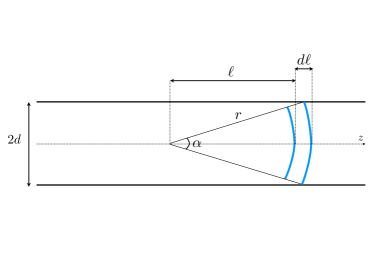
Figure 1: Schematic representation of the section of a cylindrical tube with transonic flow. The blue curves represent the acoustic horizon during phonon emission, causing the horizon’s radial fluctuation with its slight reduction between the blue lines, followed by a corresponding increase of the phonon density in the volume within the two.

As an example, in Fig. 1 we schematically show the variation of the acoustic horizon for a flow in a cylindrical tube of diameter $2d$ and axis in the $z$-direction. For a viscous fluid, the effective area of the acoustic horizon can be approximated by $A=c_{s}\alpha r^{2}$, where $r=\sqrt{d^{2}+\ell^{2}}$; for an unviscous flow, the acoustic horizon becomes flat corresponding to the $\ell\to 0$ limit. Assuming that the phonon emission happens by a horizon radial fluctuation and that it is possible to associate to the acoustic horizon an entropy as in BHs, the entropy change of the fluid is

$$dS_{H}=\frac{2\kappa\alpha c_{s}\ell d\ell}{L_{c}^{2}}\,,$$ (44)

while the associated change in the phonon entropy is

$$dS_{\text{ph}}=dV\tilde{s}_{\text{ph}}=c_{s}\alpha\ell^{2}d\ell\tilde{s}_{\text{ph}}\,.$$ (45)

Equating $dS_{H}=dS_{\text{ph}}$ and using the phonon entropy density in Eq. (39), we obtain $\displaystyle{T=\frac{2\kappa K_{+}}{\pi d_{g}\ell}}$ and

$$\lim_{\ell\to 0}T=\frac{2\kappa}{\pi}\left.\frac{\partial}{\partial z}\left(\frac{c_{s}-|v|}{1-c_{s}|v|}\right)\right|_{H}\,,$$ (46)

that is the same expression of the Hawking temperature reported in Eq. (41). As for the spherical case, we obtain the same expression of the Hawking temperature when equating the energy loss of the AH and the energy gain of the phonon gas. The present derivation can be straightforwardly extended to reduced space dimensions, e.g. in 2D, by appropriately counting the corresponding number of phonon modes.

V Conclusions

We have shown how for AHs the Hawking temperature comes with a conceptually simple covariant kinetic theory approach. Under the hypothesis that the BH and AH entropies have the analogous physical origin, we associate to the latter the entropy $A/4$ in terms of the horizon surface area $A$. Then, we determine the Hawking temperature by equating the entropy loss of the fluid with the phonon entropy gain. The same result can be obtained associating to an AH a a mass equal to half the Schwarzschild radius and equating the energy loss of the fluid with the energy gain of the phonon gas. These results hold if the horizon fluctuates radially, which is appropriate for sonic wave emission.

Our findings elucidate the relationship between the fluid fluctuations and the phonon (Hawking) emission gas variations, further clarifying the geometrical nature of the process. Remarkably, our results do not depend on the phonon emission mechanism and are truly shaped only by the geometrical properties of the acoustic horizon, as clearly emerges from our covariant description. However, the proposed method works only in a region sufficiently close to the acoustic horizon, where the system is effectively $1+1$ dimensional, and for a fluid temperature much lower than $T_{H}$. In this case, it is possible to neglect phonon-phonon interactions, meaning that the spontaneously emitted phonon gas is in a out-of-equilibrium thermodynamic state  [34].

Interestingly, we are also able to clarify an important aspect of BH physics: the spontaneous emission of photons at the event horizon should result in energy and entropy gains of the photon gas equal to the mass and entropy losses of the BH. In this case though, one complication arises because of the long-range behavior of the gravitational interaction, which may not allow to separate the photon energy density and entropy from the BH ones [2].

The physics described here can be probed in currently available experimental setups based on extremely accurate control of table-top quantum technologies, such as ultracold gases platforms. In particular, we envisage that the 2D, disk-shaped geometry setup experimented in [35, 36] can be especially promising in probing the behavior we describe. In the experiment, a coherent Hawking radiation is simulated in a 2D Bose-Einstein condensate after modulating the scattering length driving the atomic interactions, and thus the speed of sound, by a variable amount of time. The measured probability distribution of the matter-wave emission is observed to be thermal. Adapting Eqs. (36) and (43) to the desired geometry one can compute the rate of entropy as well as of energy emitted by the AH. These quantities could be measured by experimental strategy adopted in  [37] or via measurements of dynamical correlation functions [38]. In this measurement one should take into account the bulk temperature of the system, here neglected, as well as the transport properties of the superfluid. Quite generally, the theoretical framework here developed opens to new formulations of the AH physics with unexplored perspective, shining a different light on the treatment dynamical and dissipative effects.

Appendix A Dimensional reduction close to the acoustic horizon

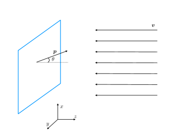
Figure 2: Schematic representation of the emission of a phonon close to the acoustic horizon. The blue rectangle corresponds to the local surface of the acoustic horizon orthogonal to the fluid velocity $\bm{v}$, which is along the $z$ axis. The black line corresponds to the emitted phonon with momentum ${\bm{p}}$ at a certain angle $\theta$ with respect to the normal to the surface. Only phonons emitted with vanishing $\bm{p}_{x}$ and $\bm{p}_{y}$ components can escape from the acoustic horizon.

The acoustic horizon is the region where the fluid velocity equals the speed of sound [1, 2, 7]. Since phonons propagate at the speed of sound, the only phonons that can escape from the acoustic horizon are those having velocity with vanishing azimuthal angle with respect to the fluid motion, corresponding to vanishing values of $\theta$ in Fig. 2, where the horizon is pictorially represented by the blue contour. In fluids, the phonon momentum and velocity are parallel, thus only those phonons emitted with vanishing $p_{x}$ and $p_{y}$ components can escape. We can interpret this result assuming that the distribution function of phonons close to the horizon of Fig. 2 is given by

$$f_{\text{ph}}=f\cdot f_{t}(p_{x},p_{y})\,,$$ (47)

where $f$ is the standard Bose-Einstein distribution (see Eq. (15)), while the $f_{t}$ distribution should in principle be derived by the microscopic physics. However, sufficiently close to the acoustic horizon $f_{t}$ can only depend on the cutoff length scale $L_{c}$, which is the only relevant length scale. For this reason we assume that sufficiently close to the horizon of Fig. 2 the transverse distribution function is given by

$$f_{t}(p_{x},p_{y})=\frac{2\pi}{L_{c}}\delta(p_{x})\frac{2\pi}{L_{c}}\delta(p_{y})\,.$$ (48)

This expression can be generalized as

$$f_{t}(p_{t})=\left(\frac{2\pi}{L_{c}}\right)^{2}\delta(p_{t}^{2})\,$$ (49)

close to any acoustic horizon, where $p_{t}$ is the transverse momentum with respect to the local orientation of $\bm{v}$ at the horizon, while we will indicate with $p^{r}$ the momentum parallel to $\bm{v}$. Instead of the Dirac delta function, one may consider a Gaussian distribution or any representation of the Dirac delta function, the results would be qualitatively the same. In any case, this would be still consistent with our kinetic theory approach (see Eq. (14)). When evaluating the energy-momentum tensor (see for instance [22])

$$T^{\alpha\beta}_{\rm ph}=\int p^{\alpha}p^{\beta}f_{\text{ph}}(p)d{\cal P}\ ,$$ (50)

the momentum measure [17, 18]

$$d{\cal P}=\sqrt{-g}2H(p)\delta({g}_{\mu\nu}p^{\mu}p^{\nu})\frac{dp^{0}dp^{r}dp_{t}^{2}}{(2\pi)^{3}}\,,$$ (51)

can be simplified by integrating out the transverse momentum. Taking into account that $\sqrt{-g}=c_{s}$, the resulting integration measure is

$$d{\cal P}=c_{s}2H(p)\delta({\tilde{g}}_{\mu\nu}p^{\mu}p^{\nu})\frac{dp^{0}dp^{r}}{(2\pi)L_{c}^{2}}\,,$$ (52)

where ${\tilde{g}}_{\mu\nu}$ is the two-dimensional metric. This expression can be rewritten as

$$d{\cal P}=c_{s}\frac{\delta(p_{0}-E_{+})}{p^{0}}\frac{dp^{0}dp^{r}}{(2\pi)L_{c}^{2}}\,,$$ (53)

where $E_{+}$ is the dispersion law of phonons. The latter can be obtained from $g^{\mu\nu}p_{\mu}p_{\nu}=0$ and has the general expression

$$E_{\pm}=\frac{vp_{r}(1-c_{s}^{2})\pm c_{s}\gamma^{-2}\sqrt{p_{t}^{2}\gamma^{2}(1-c_{s}^{2}v^{2})+p_{r}^{2}}}{1-c_{s}^{2}v^{2}}\,,$$ (54)

which for vanishing transverse momenta gives

$$E_{\pm}=\frac{v\pm c_{s}}{1\pm vc_{s}}p_{r}=K_{\pm}p_{r}\,,$$ (55)

with the $+$ sign corresponding to the positive energy states relevant for the kinetic equations.

Appendix B Evaluation of the thermodynamic quantities

From the expression of the energy-momentum tensor in Eq. (50) and using the integration measure in Eq. (53) we can extract the energy density

$$\tilde{\epsilon}_{\text{ph}}=\sqrt{-g}T^{0}_{\phantom{0}0}=\int E_{+}f\frac{dp_{r}}{2\pi L_{c}^{2}}\,,$$ (56)

where

$$f=\frac{1}{e^{K_{+}p_{r}/T}-1}\,,$$ (57)

is the phonon distribution function. Similarly, the pressure can be evaluated by using

$$\sqrt{-g}T^{i}_{\phantom{i}j}=\delta^{ir}\delta_{jr}\tilde{P}_{\text{ph}}\,,$$ (58)

showing that the pressure is radially oriented: it is locally orthogonal to the acoustic horizon. We can derive the entropy density by the thermodynamic relation

$$\tilde{\epsilon}_{\text{ph}}+\tilde{P}_{\text{ph}}=T\tilde{s}_{\text{ph}}\,,$$ (59)

which holds because phonons are emitted at the temperature, $T$, and they have vanishing chemical potential. Since $\tilde{P}_{\text{ph}}=\tilde{\epsilon}_{\text{ph}}$, we obtain that

$$T\tilde{s}_{\text{ph}}=2\tilde{\epsilon}_{\text{ph}}\,,$$

and upon changing the integration variable to $x=K_{+}p/T$, Eq. (56) yields

$$\tilde{\epsilon}_{\text{ph}}=\frac{T^{2}}{2\pi L_{c}^{2}K_{+}}\int_{0}^{\infty}xf(x)dx\,.$$ (60)

Since

$$\int_{0}^{\infty}xf(x)dx=\frac{\pi^{2}}{6}\,,$$ (61)

it follows that

$$\tilde{s}_{\text{ph}}=\frac{\pi T}{6L_{c}^{2}K_{+}}\,.$$ (62)

Alternatively, the entropy density can be evaluated using the expression

$$s_{\rm ph}=-c_{s}\int\left[f\ln{f}-(1+f)\ln{(1+f)}\right]\delta(p_{0}-E_{+})\frac{dp^{0}dp^{r}}{(2\pi)L_{c}^{2}}\,,$$ (63)

and upon lowering the indices in the integration measure, which amounts to divide by $c_{s}^{2}$, and integrating over $p_{0}$ we obtain

$$s_{\rm ph}=-\frac{1}{c_{s}}\int\left[f\ln{f}-(1+f)\ln{(1+f)}\right]\frac{dp_{r}}{(2\pi)L_{c}^{2}}\,,$$ (64)

where the distribution function is in Eq. (57). Upon changing the integration variable to $x=K_{+}p_{r}/T$, we get

$$s_{\rm ph}=-\frac{T}{(2\pi)L_{c}^{2}K_{+}c_{s}}\int\left[f\ln{f}-(1+f)\ln{(1+f)}\right]dx\,,$$ (65)

where the integral can now be analytically evaluated to

$$\int\left[f\ln{f}-(1+f)\ln{(1+f)}\right]dx=-\frac{\pi^{2}}{3}\,,$$ (66)

meaning that the entropy density $\tilde{s}_{\text{ph}}=\sqrt{-g}s_{\text{ph}}$, takes the expression in Eq. (62). Noticeably, for $r\rightarrow r_{H}$, the factor $K_{+}$ introduces a divergence in the energy and enetropy densities, meaning that we are approaching the phonon source. However, the covariant entropy and energy density in Eqs. (56) and (62) can be regularized by the short distance cutoff $L_{c}$. This is evident from (54), accounting for the finite value of the transverse momentum $p_{t}\sim 1/L_{c}^{2}$, hence removing the divergence that appears in the energy and entropy densities due to the vanishing of $K_{+}$ at the acoustic horizon. The non-vanishing transverse momentum can be related to dissipative effects, which transfer momentum in the orthogonal direction with respect to the flow. This shows that dissipation can effectively regularize the behaviour close to the horizon. We shall come back on this issue in a separate work.

References

- Unruh [1981] W. Unruh, Experimental black hole evaporation, Phys.Rev.Lett. 46, 1351 (1981).
- Brout et al. [1995] R. Brout, S. Massar, R. Parentani, and P. Spindel, A Primer for black hole quantum physics, Phys. Rept. 260, 329 (1995), arXiv:0710.4345 [gr-qc] .
- Corley [1998] S. Corley, Computing the spectrum of black hole radiation in the presence of high frequency dispersion: An Analytical approach, Phys. Rev. D 57, 6280 (1998), arXiv:hep-th/9710075 .
- Saida and Sakagami [2000] H. Saida and M.-a. Sakagami, Black hole radiation with high frequency dispersion, Phys. Rev. D 61, 084023 (2000), arXiv:gr-qc/9905034 .
- Himemoto and Tanaka [2000] Y. Himemoto and T. Tanaka, Generalization of the model of Hawking radiation with modified high frequency dispersion relation, in 9th M. Grossmann Meeting on Recent Developments in Theoretical and Experimental General Relativity, Gravitation and Relativistic Field Theories (2000) pp. 1384–1394.
- Unruh and Schutzhold [2005] W. G. Unruh and R. Schutzhold, On the universality of the Hawking effect, Phys. Rev. D 71, 024028 (2005), arXiv:gr-qc/0408009 .
- Barcelo et al. [2005] C. Barcelo, S. Liberati, and M. Visser, Analogue gravity, Living Rev. Rel. 8, 12 (2005), arXiv:gr-qc/0505065 .
- Balbinot et al. [2005] R. Balbinot, A. Fabbri, S. Fagnocchi, and R. Parentani, Hawking radiation from acoustic black holes, short distance and back-reaction effects, Riv. Nuovo Cim. 28, 1 (2005), arXiv:gr-qc/0601079 .
- Carusotto et al. [2008] I. Carusotto, S. Fagnocchi, A. Recati, R. Balbinot, and A. Fabbri, Numerical observation of Hawking radiation from acoustic black holes in atomic Bose–Einstein condensates, New J. Phys. 10, 103001 (2008), 0803.0507 .
- Steinhauer [2016] J. Steinhauer, Observation of quantum Hawking radiation and its entanglement in an analogue black hole, Nature Physics 12, 959–965 (2016).
- Muñoz de Nova et al. [2019] J. R. Muñoz de Nova, K. Golubkov, V. I. Kolobov, and J. Steinhauer, Observation of thermal Hawking radiation and its temperature in an analogue black hole, Nature 569, 688 (2019).
- Stone [2000] M. Stone, Acoustic energy and momentum in a moving medium, Physical Review E 62, 1341 (2000).
- Volovik [2001] G. Volovik, Superfluid analogies of cosmological phenomena, Phys. Rept. 351, 195 (2001), arXiv:gr-qc/0005091 .
- Bardeen et al. [1973] J. M. Bardeen, B. Carter, and S. W. Hawking, The four laws of black hole mechanics, Comm. Math. Phys. 31, 161 (1973).
- Bekenstein [1973] J. D. Bekenstein, Black holes and entropy, Phys. Rev. D 7, 2333 (1973).
- Jacobson [1994] T. Jacobson, Black hole entropy and induced gravity (1994), arXiv:gr-qc/9404039 .
- Lindquist [1966] R. W. Lindquist, Relativistic transport theory, Annals of Physics 37, 487 (1966).
- Stewart [1969] J. Stewart, Lecture Notes in Physics, Lecture Notes in Physics No. v. 10 (Springer-Verlag, 1969).
- Leutwyler [1997] H. Leutwyler, Phonons as goldstone bosons, Helv. Phys. Acta 70, 275 (1997), arXiv:hep-ph/9609466 [hep-ph] .
- Schakel [1996] A. M. Schakel, Effective field theory of ideal-fluid hydrodynamics, Modern Physics Letters B 10, 999 (1996).
- Son [2002] D. T. Son, Low-energy quantum effective action for relativistic superfluids (2002), arXiv:hep-ph/0204199 [hep-ph] .
- Mannarelli and Manuel [2008] M. Mannarelli and C. Manuel, Transport theory for cold relativistic superfluids from an analogue model of gravity, Phys. Rev. D 77, 103014 (2008), arXiv:0802.0321 [hep-ph] .
- Manuel and Llanes-Estrada [2007] C. Manuel and F. J. Llanes-Estrada, Bulk viscosity in a cold CFL superfluid, JCAP 08, 001, arXiv:0705.3909 [hep-ph] .
- Bilic [1999] N. Bilic, Relativistic acoustic geometry, Class. Quant. Grav. 16, 3953 (1999), arXiv:gr-qc/9908002 .
- Visser and Molina-Paris [2010] M. Visser and C. Molina-Paris, Acoustic geometry for general relativistic barotropic irrotational fluid flow, New J. Phys. 12, 095014 (2010), arXiv:1001.1310 [gr-qc] .
- Jacobson [1991] T. Jacobson, Black hole evaporation and ultrashort distances, Phys. Rev. D 44, 1731 (1991).
- Macher and Parentani [2009a] J. Macher and R. Parentani, Black hole radiation in Bose-Einstein condensates, Phys. Rev. A 80, 043601 (2009a), arXiv:0905.3634 [cond-mat.quant-gas] .
- Macher and Parentani [2009b] J. Macher and R. Parentani, Black/White hole radiation from dispersive theories, Phys. Rev. D 79, 124008 (2009b), arXiv:0903.2224 [hep-th] .
- Eardley and Giddings [2002] D. M. Eardley and S. B. Giddings, Classical black hole production in high-energy collisions, Phys. Rev. D 66, 044011 (2002), arXiv:gr-qc/0201034 .
- Yoshino and Nambu [2003] H. Yoshino and Y. Nambu, Black hole formation in the grazing collision of high-energy particles, Phys. Rev. D 67, 024009 (2003), arXiv:gr-qc/0209003 .
- Yoshino and Rychkov [2005] H. Yoshino and V. S. Rychkov, Improved analysis of black hole formation in high-energy particle collisions, Phys. Rev. D 71, 104028 (2005), [Erratum: Phys.Rev.D 77, 089905 (2008)], arXiv:hep-th/0503171 .
- Misner et al. [1973] C. W. Misner, K. S. Thorne, and J. A. Wheeler, Gravitation (W. H. Freeman, San Francisco, 1973).
- Shapiro and Teukolsky [1983] S. Shapiro and S. Teukolsky, Black holes, white dwarfs, and neutron stars: the physics of compact objects, A Wiley-interscience publication (Wiley, New York, USA, 1983).
- Prigogine [2017] I. Prigogine, Non-Equilibrium Statistical Mechanics, Dover Books on Physics (Dover Publications, 2017).
- Clark et al. [2017] L. W. Clark, A. Gaj, L. Feng, and C. Chin, Collective emission of matter-wave jets from driven Bose-Einstein condensates, Nature 551, 356–359 (2017).
- Hu et al. [2019] J. Hu, L. Feng, Z. Zhang, and C. Chin, Quantum Simulation of Coherent Hawking-Unruh Radiation, Nature Physics 15, 785–789 (2019).
- Ku et al. [2012] M. J. H. Ku, A. T. Sommer, L. W. Cheuk, and M. W. Zwierlein, Revealing the Superfluid Lambda Transition in the Universal Thermodynamics of a Unitary Fermi Gas, Science 335, 563 (2012), arXiv:1110.3309v1 .
- [38] V. I. Kolobov, K. Golubkov, J. R. Muñoz de Nova, and J. Steinhauer, Spontaneous Hawking Radiation and Beyond: Observing the Time Evolution of an Analogue Black Hole, gr-qc/1910.09363 .