Efficient Channel Estimation for Double-IRS Aided Multi-User MIMO System

Abstract

To achieve the more significant passive beamforming gain in the double-intelligent reflecting surface (IRS) aided system over the conventional single-IRS counterpart, channel state information (CSI) is indispensable in practice but also more challenging to acquire, due to the presence of not only the single- but also double-reflection links that are intricately coupled and also entail more channel coefficients for estimation. In this paper, we propose a new and efficient channel estimation scheme for the double-IRS aided multi-user multiple-input multiple-output (MIMO) communication system to resolve the cascaded CSI of both its single- and double-reflection links. First, for the single-user case, the single- and double-reflection channels are efficiently estimated at the multi-antenna base station (BS) with both the IRSs turned ON (for maximal signal reflection), by exploiting the fact that their cascaded channel coefficients are scaled versions of their superimposed lower-dimensional CSI. Then, the proposed channel estimation scheme is extended to the multi-user case, where given an arbitrary user’s cascaded channel (estimated as in the single-user case), the other users’ cascaded channels can also be expressed as lower-dimensional scaled versions of it and thus efficiently estimated at the BS. Simulation results verify the effectiveness of the proposed channel estimation scheme and joint training reflection design for double IRSs, as compared to various benchmark schemes.

I Introduction

Intelligent reflecting surface (IRS) has recently emerged as an innovative solution to the realization of smart and reconfigurable environment for wireless communications [2, 3, 4, 5]. Specifically, IRS consists of a large number of passive reflecting elements with ultra-low power consumption, each being able to control the reflection phase shift and/or amplitude of the incident signal in a programmable manner so as to collaboratively reshape the wireless propagation channel in favor of signal transmission. As such, different from the existing transmission techniques that can only adapt to but have no control over the random wireless channels, IRS provides a new means to effectively combat with wireless channel fading impairment and co-channel interference. Furthermore, as being of light weight and free of radio frequency (RF) chains, large-scale IRSs can be densely deployed in various wireless communication systems [6, 7, 8, 9, 10, 11, 12] to enhance their performance at low as well as sustainable energy and hardware cost.

Prior works on IRS mainly considered the wireless communication systems aided by one or multiple distributed IRSs (see, e.g., [13, 14, 15, 16, 17, 18, 19, 20, 21, 22, 23]), each independently serving its nearby users without taking into account the inter-IRS signal reflection, which, however, fails to capture the cooperative beamforming gains between IRSs to further improve the system performance. Only recently, the cooperative beamforming over inter-IRS channel has been explored in the double-IRS aided communication system [24, 25, 26], which was shown to achieve a much higher-order passive beamforming gain than that of the conventional single-IRS aided system (i.e., ${\cal O}(M^{4})$ versus ${\cal O}(M^{2})$ with $M$ denoting the total number of reflecting elements/subsurfaces in both systems [24]). However, achieving this more appealing passive beamforming gain requires more channel training overhead in practice, due to the significantly more channel coefficients to be estimated over the inter-IRS double-reflection link, in addition to the single-reflection links in the conventional single-IRS system. Note that existing works on IRS channel estimation mainly focused on the channel state information (CSI) acquisition for the single-reflection links only [27, 28, 29, 30, 31, 32, 33, 34, 35, 36], which, however, are inapplicable to the double-IRS aided system with the co-existence of single- and double-reflection links as shown in Fig. 1. In [24], the authors assumed that the two IRSs in the double-IRS system are equipped with receive RF chains to enable signal sensing for estimating their channels with the base station (BS)/user, separately. However, even with receive RF chains integrated to IRSs, the channel estimation for the inter-IRS (i.e., IRS 1$\rightarrow$IRS 2 in Fig.1) link still remains a difficult task in practice (unless active sensors that can both transmit and receive signals are mounted on the IRSs, which inevitably incurs additional hardware cost and complexity). In contrast, the double-IRS channel estimation with fully-passive IRSs was investigated in [26], but without the single-reflection links considered and for the single-user case only. In [1], we presented a decoupled channel estimation scheme for the general double-IRS aided system with multiple BS antennas/users, which successively estimates the two single-reflection channels (each corresponding to one of the two IRSs turned ON with the other turned OFF, respectively) and then the double-reflection channel (with the signals canceled over the two single-reflection channels estimated) in a decoupled manner. Although this scheme substantially reduces the training overhead of that in [26], it suffers from not only residual interference due to imperfect signal cancellation (based on the estimated single-reflection channels) but also considerable reflection power loss due to the ON/OFF reflection control of the two IRSs during the channel training, which thus degrade the channel estimation accuracy.

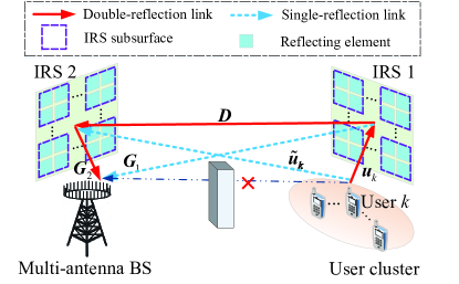
Figure 1: A double-IRS cooperatively aided multi-user MIMO communication system in the uplink.

To overcome the above issues, we propose in this paper a new and efficient channel estimation scheme for the double-IRS aided multi-user multiple-input multiple-output (MIMO) communication system shown in Fig. 1, where two fully-passive IRSs are deployed near a multi-antenna BS and a cluster of $K$ users, respectively, to assist their communications. Different from the decoupled channel estimation scheme in [1], we propose to jointly estimate the cascaded CSI of the single- and double-reflection links with the always-ON training reflection (i.e., all the reflecting elements/subsurfaces of the two IRSs are switched ON with the maximum reflection amplitude during the entire channel training) while properly tuning their reflection phase-shifts over time, which thus achieves the full-reflection power for improving the channel estimation accuracy significantly. Note that with the always-ON reflection of both IRSs, the two single-reflection channels (each corresponding to one of the two IRSs, respectively) are superimposed with the double-reflection channel at all time, which makes them difficult to be estimated separately at the BS based on the received user pilot signals over the intricately coupled single- and double-reflection links. To tackle this difficulty, we explore the intrinsic relationship between the single- and double-reflection channels as well as that among different users and design the training reflection phase-shifts of the two IRSs accordingly to achieve low training overhead and yet high channel estimation accuracy. Specifically, the main contributions of this paper are summarized as follows (please refer to Fig. 1 for the channel illustration).

• First, for the single-user case, the superimposed CSI of the single- and double-reflection channels related to IRS 2 is estimated at the multi-antenna BS with dynamically tuned reflection phase-shifts of IRS 2 over time and those of IRS 1 being fixed. Then, the high-dimensional double-reflection (i.e., user$\rightarrow$IRS 1$\rightarrow$IRS 2$\rightarrow$BS) channel and the single-reflection (i.e., user$\rightarrow$IRS 2$\rightarrow$BS) channel are efficiently estimated, by exploiting the fact that their cascaded channel coefficients are scaled versions of their superimposed CSI due to their commonly shared IRS 2$\rightarrow$BS link; as a result, by taking the superimposed CSI as the reference CSI, only the lower-dimensional scaling factors and the other single-reflection (i.e., user$\rightarrow$IRS 1$\rightarrow$BS) channel need to be estimated at the multi-antenna BS, thus greatly reducing the training overhead. The proposed channel estimation scheme is further extended to the multi-user case, where given an arbitrary user’s cascaded channel estimated as in the single-user case, the other users’ cascaded channels are also (lower-dimensional) scaled versions of it and thus can be efficiently estimated at the BS with low training overhead.

• Moreover, for the proposed channel estimation scheme, we jointly optimize the training reflection phase-shifts of the two IRSs to minimize the channel estimation error over different training phases, for which some closed-form optimal solutions are derived with desired orthogonality. In addition, we analytically characterize the minimum training overhead of the proposed scheme, which is shown to decrease with the increasing number of BS antennas $N$ until reaching its lower bound with $N>M$. We also show an interesting trade-off in training time allocation over different training phases with the intricate error propagation effect taken into account.

• Last, we provide extensive numerical results to validate the superiority of our proposed channel estimation scheme to other benchmark schemes in terms of both training overhead and channel estimation error. Besides, the effectiveness of the proposed joint training reflection phase-shift design for double IRSs is also corroborated by simulation results, as compared to other heuristic training reflection designs.

The rest of this paper is organized as follows. Section II presents the system model for the double-IRS aided multi-user MIMO system. In Sections III and IV, we propose efficient channel estimation schemes with optimized training reflection phase-shift designs for the single-user and multi-user cases, respectively. Simulation results are presented in Section V to evaluate the performance of the proposed channel estimation scheme and training reflection phase-shift design. Finally, conclusions are drawn in Section VI.

Notation: Upper-case and lower-case boldface letters denote matrices and column vectors, respectively. Superscripts ${\left(\cdot\right)}^{T}$, ${\left(\cdot\right)}^{H}$, ${\left(\cdot\right)}^{*}$ ${\left(\cdot\right)}^{-1}$, and ${\left(\cdot\right)}^{\dagger}$ stand for the transpose, Hermitian transpose, conjugate, matrix inversion, and pseudo-inverse operations, respectively. ${\mathbb{C}}^{a\times b}$ denotes the space of ${a\times b}$ complex-valued matrices. For a complex-valued vector $\bm{x}$, $\lVert\bm{x}\rVert$ denotes its $\ell_{2}$-norm and $\mathrm{diag}(\bm{x})$ returns a diagonal matrix with the elements in $\bm{x}$ on its main diagonal. For a general matrix ${\bm{A}}$, ${\rm rank}\left({\bm{A}}\right)$ returns its rank, $\left\|{\bm{A}}\cdot\right\|_{F}$ denotes its Frobenius norm, ${\rm vec}\left({\bm{A}}\right)$ denotes the vectorization of ${\bm{A}}$ by stacking its columns into a column vector, and $[{\bm{A}}]_{a:b,c:d}$ denotes the submatrix of ${\bm{A}}$ with its rows from $a$ to $b$ and columns from $c$ to $d$. ${\cal O}(\cdot)$ denotes the standard big-O notation, $\lceil\cdot\rceil$ is the ceiling function, $\otimes$ denotes the Kronecker product, and ${\mathbb{E}}\{\cdot\}$ stands for the statistical expectation. ${\bm{I}}$, ${\bm{1}}$, and ${\bm{0}}$ denote an identity matrix, an all-one vector/matrix, and an all-zero vector/matrix, respectively, with appropriate dimensions. The distribution of a circularly symmetric complex Gaussian (CSCG) random vector with mean vector $\bm{\mu}$ and covariance matrix ${\bm{\Sigma}}$ is denoted by ${\mathcal{N}_{c}}({\bm{\mu}},{\bm{\Sigma}})$; and $\sim$ stands for “distributed as”.

II System Model

Consider a double-IRS cooperatively aided multi-user MIMO communication system shown in Fig. 1, in which two distributed IRSs (referred to as IRS 1 and IRS 2) are deployed to assist the communications between a cluster of $K$ single-antenna users and an $N$-antenna BS. As in [25], we consider a practical scenario where the direct links between the users in the cluster of interest and the BS are severely blocked due to obstacles (e.g., walls/corners in the indoor environment) and thus can be ignored. To bypass the blockage as well as minimize the path loss, IRSs 1 and 2 are properly placed near the cluster of users and the BS, respectively, such that the $K$ users can be effectively served by the BS through both the single- and double-reflection links created by them. Let $M$ denote our budget on the total number of passive subsurfaces for the two distributed IRSs, where IRSs 1 and 2 comprise $M_{1}$ and $M_{2}$ subsurfaces, respectively, with $M_{1}+M_{2}=M$. Similar to the element-grouping strategy in [37, 27], each of these IRS subsurfaces is composed of an arbitrary number of adjacent reflecting elements that share a common phase shift for reducing the channel estimation and reflection design complexity. In this paper, we assume the quasi-static flat-fading channel model for all channels involved, which remain approximately constant during each channel coherence interval.

Let ${{\bm{u}}}_{k}\triangleq\left[u_{k,1},\ldots,u_{k,M_{1}}\right]^{T}\in{\mathbb{C}^{M_{1}\times 1}}$, ${\tilde{\bm{u}}}_{k}\triangleq\left[{\tilde{u}}_{k,1},\ldots,{\tilde{u}}_{k,M_{2}}\right]^{T}\in{\mathbb{C}^{M_{2}\times 1}}$, ${{\bm{D}}}\triangleq\left[{\bm{d}}_{1},\ldots,{\bm{d}}_{M_{1}}\right]\in{\mathbb{C}^{M_{2}\times M_{1}}}$, ${{\bm{G}}}_{1}\in{\mathbb{C}^{N\times M_{1}}}$, and ${{\bm{G}}}_{2}\in{\mathbb{C}^{N\times M_{2}}}$ denote the baseband equivalent channels in the uplink for the user $k$$\rightarrow$IRS 1, user $k$$\rightarrow$IRS 2, IRS 1$\rightarrow$IRS 2, IRS 1$\rightarrow$BS, and IRS 2$\rightarrow$BS links, respectively, with $k=1,\ldots,K$. Let ${\bm{\theta}}_{\mu}\triangleq[{\theta_{\mu,1}},\ldots,{\theta_{\mu,M_{\mu}}}]^{T}=\left[\beta_{\mu,1}e^{j\phi_{\mu,1}},\ldots,\beta_{\mu,M_{\mu}}e^{j\phi_{\mu,M_{\mu}}}\right]^{T}\in{\mathbb{C}^{M_{\mu}\times 1}}$ denote the equivalent reflection coefficients of IRS $\mu$ with $\mu\in\{1,2\}$, where $\beta_{\mu,m}\in[0,1]$ and $\phi_{\mu,m}\in[0,2\pi)$ are the reflection amplitude and phase shift of subsurface $m$ at IRS $\mu$, respectively. Thus, the effective channel from user $k$ to the BS is the superimposition of the double-reflection link and the two single-reflection links (see Fig. 1), which is given by

$${\bm{h}}_{k}= {{\bm{G}}}_{2}{\bm{\Phi}}_{2}{{\bm{D}}}{\bm{\Phi}}_{1}{{\bm{u}}}_{k}+{{\bm{G}}}_{2}{\bm{\Phi}}_{2}{\tilde{\bm{u}}}_{k}+{{\bm{G}}}_{1}{\bm{\Phi}}_{1}{{\bm{u}}}_{k}$$ (1)

where ${\bm{\Phi}}_{\mu}={\rm diag}\left({\bm{\theta}}_{\mu}\right)$ denotes the diagonal reflection matrix of IRS $\mu$ with $\mu\in\{1,2\}$. With fully-passive IRSs 1 and 2, it is infeasible to acquire the CSI between the two IRSs as well as that with the BS/users separately. Nonetheless, it was shown in [25] that the cascaded CSI (to be specified below) is sufficient for designing the cooperative reflection/passive beamforming at the two IRSs to maximize the data transmission rate without loss of optimality. As such, let ${{\bm{R}}}_{k}={{\bm{G}}}_{1}{\rm diag}\left({{\bm{u}}}_{k}\right)\in{\mathbb{C}^{N\times M_{1}}}$ (${\tilde{\bm{R}}}_{k}={{\bm{G}}}_{2}{\rm diag}\left({\tilde{\bm{u}}}_{k}\right)\in{\mathbb{C}^{N\times M_{2}}}$) denote the cascaded user $k$$\rightarrow$IRS 1 (IRS 2)$\rightarrow$BS channel (without taking the effect of IRS reflection yet) for the single-reflection link reflected by IRS 1 (IRS 2), and ${\tilde{\bm{D}}}_{k}\triangleq\left[{\tilde{\bm{d}}}_{k,1},\ldots,{\tilde{\bm{d}}}_{k,M_{1}}\right]={{\bm{D}}}{\rm diag}\left({{\bm{u}}}_{k}\right)\in{\mathbb{C}^{M_{2}\times M_{1}}}$ denote the cascaded user $k$$\rightarrow$IRS 1$\rightarrow$ IRS 2 channel (without IRS reflection) with ${\tilde{\bm{d}}}_{k,m}={\bm{d}}_{m}{{u}}_{k,m}\in{\mathbb{C}^{M_{2}\times 1}},\forall m=1,\ldots,M_{1}$. Then, the channel model in (1) can be equivalently expressed as

$${\bm{h}}_{k} ={{\bm{G}}}_{2}{\bm{\Phi}}_{2}{\tilde{\bm{D}}}_{k}{\bm{\theta}}_{1}+{\tilde{\bm{R}}}_{k}{\bm{\theta}}_{2}+{{\bm{R}}}_{k}{\bm{\theta}}_{1}$$

$$={{\bm{G}}}_{2}\left[{\bm{\Phi}}_{2}{\tilde{\bm{d}}}_{k,1},\ldots,{\bm{\Phi}}_{2}{\tilde{\bm{d}}}_{k,M_{1}}\right]{\bm{\theta}}_{1}+{\tilde{\bm{R}}}_{k}{\bm{\theta}}_{2}+{{\bm{R}}}_{k}{\bm{\theta}}_{1}$$

$$={{\bm{G}}}_{2}\left[{\rm diag}\left({\tilde{\bm{d}}}_{k,1}\right){\bm{\theta}}_{2},\ldots,{\rm diag}\left({\tilde{\bm{d}}}_{k,M_{1}}\right){\bm{\theta}}_{2}\right]{{\bm{\theta}}}_{1}$$

$$~{}~{}~{}+{\tilde{\bm{R}}}_{k}{\bm{\theta}}_{2}+{{\bm{R}}}_{k}{\bm{\theta}}_{1}$$

$$=\sum\limits_{m=1}^{M_{1}}\underbrace{{{\bm{G}}}_{2}~{}{\rm diag}\left({\tilde{\bm{d}}}_{k,m}\right)}_{{{\bm{Q}}}_{k,m}}{\bm{\theta}}_{2}{\theta}_{1,m}+{\tilde{\bm{R}}}_{k}{\bm{\theta}}_{2}+{{\bm{R}}}_{k}{\bm{\theta}}_{1}$$ (2)

where ${{\bm{Q}}}_{k,m}\in{\mathbb{C}^{N\times M_{2}}}$ denotes the cascaded user $k$$\rightarrow$IRS 1$\rightarrow$IRS 2$\rightarrow$BS channel associated with subsurface $m$ of IRS 1, $\forall m=1,\ldots,M_{1}$ for the double-reflection link. According to (2), it is sufficient to acquire the knowledge of the cascaded channels $\left\{{{\bm{Q}}}_{k,m}\right\}_{m=1}^{M_{1}}$, ${\tilde{\bm{R}}}_{k}$, and ${{\bm{R}}}_{k}$ for jointly designing the passive beamforming $\left\{{\bm{\theta}}_{1},{\bm{\theta}}_{2}\right\}$ for uplink/downlink data transmission in the double-IRS aided multi-user MIMO system, which is applicable to, but not limited to, the max-min SINR problem considered in [25].

However, the total number of channel coefficients in the cascaded channels $\left\{{{\bm{Q}}}_{k,m}\right\}_{m=1}^{M_{1}}$, ${\tilde{\bm{R}}}_{k}$, and ${{\bm{R}}}_{k}$ is prohibitively large, which consists of two parts:

• The number of channel coefficients (equal to $K\times NM_{1}M_{2}$) for the high-dimensional double-reflection link (i.e., $\left\{{{\bm{Q}}}_{k,m}\right\}_{m=1}^{M_{1}}$), which are newly introduced due to the double IRSs.

• The number of channel coefficients (equal to $K\times N(M_{1}+M_{2})$) for the two single-reflection links (i.e., ${{\bm{R}}}_{k}$ and ${\tilde{\bm{R}}}_{k}$), which exist in the conventional single-IRS aided system (with either IRS 1 or IRS 2 present).

As such, the number of channel coefficients for the double-reflection link is of much higher-order than that for the two single-reflection links due to the fact that $M_{1}M_{2}\gg M_{1}+M_{2}$ given large $M_{1}$ and $M_{2}$ in practice, which makes the channel estimation problem more challenging for the double-IRS aided system, as compared to the single-IRS counterpart. Note that given a limited channel coherence interval, such a considerably larger number of channel coefficients may require significantly more training overhead that renders much less or even no time for data transmission, thus resulting in reduced achievable rate for the double-IRS aided system (despite the higher-order passive beamforming gain over the double-reflection link assuming perfect CSI as shown in [25]). Moreover, the cascaded CSI of the double-refection link needs to be efficiently estimated along with that of the two single-reflection links. However, the pilot signals from the users are intricately coupled over the single- and double-reflection links when both the two IRSs are turned ON for maximizing the reflected signal power, which thus calls for new designs for their joint channel estimation at the multi-antenna BS.

To tackle the above challenges, we propose a new and efficient channel estimation scheme for the considered double-IRS aided system that achieves practically low training overhead and yet high channel estimation accuracy. We first consider the single-user setup, i.e., $K=1$, to illustrate the main idea of the proposed channel estimation scheme and training reflection design in Section III, and then extend the results to the general multi-user case in Section IV. To reduce the hardware cost and maximize the signal reflection power, we consider the always-ON training reflection design for which all the reflecting elements/sub-surfaces at the two IRSs are turned ON during the entire channel training and their reflection amplitudes are set to the maximum value of one (i.e., $\beta_{\mu,m}=1,\forall m=1,\ldots,M_{\mu},\mu\in\{1,2\}$), and thereby focus on the dynamically tuned reflection phase-shift design for achieving efficient joint channel estimation of the single- and double-reflection links.

III Double-IRS Channel Estimation for Single-User Case

In this section, we study the cascaded channel estimation and training design for the single-user case with $K=1$. For notational convenience, the user index $k$ is omitted in this section.

III-A Proposed Channel Estimation Scheme

Note that with both IRSs 1 and 2 turned ON simultaneously, the double-reflection channel $\left\{{{\bm{Q}}}_{m}\right\}_{m=1}^{M_{1}}$ and two single-reflection channels $\left\{{{\bm{R}}},{\tilde{\bm{R}}}\right\}$ are superimposed in (2), which are difficult to be estimated separately at the BS as the received pilot signals from the user are intricately coupled over the single- and double-reflection links. To tackle this difficulty, we propose an efficient channel estimation scheme, which includes two phases as elaborated below.

Phase I: In this phase, we fix the reflection phase-shifts of IRS 1, i.e., ${\bm{\theta}}_{1,\rm I}^{(i)}={\bm{\theta}}_{1,\rm I},\forall i=1,\ldots,I_{1}$ and dynamically tune the reflection phase-shifts of IRS 2, i.e., ${\bm{\theta}}_{2,\rm I}^{(i)}$, over different pilot symbols to facilitate the cascaded channel estimation, where $I_{1}$ denotes the number of pilot symbols in Phase I. For simplicity, we set ${\bm{\theta}}_{1,\rm I}={\bm{1}}_{M_{1}\times 1}$ and thus the effective channel in (2) during symbol $i$ of Phase I, denoted by ${\bm{h}}_{\rm I}^{(i)}$, is given by

$${\bm{h}}_{\rm I}^{(i)} =\sum_{m=1}^{M_{1}}{{\bm{Q}}}_{m}{\bm{\theta}}_{2,\rm I}^{(i)}+{\tilde{\bm{R}}}{\bm{\theta}}_{2,\rm I}^{(i)}+{{\bm{G}}}_{1}{{\bm{u}}}$$

$$=\sum\limits_{m=1}^{M_{1}}{{\bm{G}}}_{2}~{}{\rm diag}\left({\tilde{\bm{d}}}_{m}\right){\bm{\theta}}_{2,\rm I}^{(i)}+{{\bm{G}}}_{2}{\rm diag}\left({\tilde{\bm{u}}}\right){\bm{\theta}}_{2,\rm I}^{(i)}+{{\bm{G}}}_{1}{{\bm{u}}}$$

$$={{\bm{G}}}_{2}{\rm diag}\left({\tilde{\bm{u}}}+\sum_{m=1}^{M_{1}}{\tilde{\bm{d}}}_{m}\right){\bm{\theta}}_{2,\rm I}^{(i)}+{{\bm{G}}}_{1}{{\bm{u}}},i=1,\ldots,I_{1}.$$ (3)

For notational convenience, we let ${\bm{g}}_{1}\triangleq{{\bm{G}}}_{1}{{\bm{u}}}\in{\mathbb{C}^{N\times 1}}$, ${\bar{\bm{d}}}\triangleq{\tilde{\bm{u}}}+\sum_{m=1}^{M_{1}}{\tilde{\bm{d}}}_{m}\in{\mathbb{C}^{M_{2}\times 1}}$, and

$${\bar{\bm{Q}}}\triangleq{{\bm{G}}}_{2}~{}{\rm diag}\left({\bar{\bm{d}}}\right)={\tilde{\bm{R}}}+\sum_{m=1}^{M_{1}}{{\bm{Q}}}_{m}$$ (4)

where ${\bar{\bm{Q}}}\in{\mathbb{C}^{N\times M_{2}}}$ can be regarded as the superimposed CSI of the single- and double-reflection channels related to IRS 2. As such, the effective channel in (III-A) can be simplified as

$${\bm{h}}_{\rm I}^{(i)}={\bar{\bm{Q}}}{\bm{\theta}}_{2,\rm I}^{(i)}+{\bm{g}}_{1},\quad i=1,\ldots,I_{1}.$$ (5)

Based on the channel model in (5) with $x_{\rm I}^{(i)}=1$ being the pilot symbol transmitted by the (single) user, the received signal at the BS during symbol $i$ of Phase I is expressed as

$${\bm{z}}_{\rm I}^{(i)}={\bar{\bm{Q}}}~{}{\bm{\theta}}_{2,\rm I}^{(i)}+{\bm{g}}_{1}+{\bm{v}}_{\rm I}^{(i)},\quad i=1,\ldots,I_{1}$$ (6)

where ${\bm{v}}_{\rm I}^{(i)}\sim{\mathcal{N}_{c}}({\bm{0}},\sigma^{2}{\bm{I}}_{N})$ is the additive white Gaussian noise (AWGN) vector with normalized noise power of $\sigma^{2}$ at the BS (with respect to user transmit power). By stacking the received signal vectors $\left\{{\bm{z}}_{\rm I}^{(i)}\right\}_{i=1}^{I_{1}}$ into ${\bm{Z}}_{\rm I}=\left[{\bm{z}}_{\rm I}^{(1)},{\bm{z}}_{\rm I}^{(2)},\ldots,{\bm{z}}_{\rm I}^{(I_{1})}\right]\in{\mathbb{C}^{N\times I_{1}}}$, we obtain

$${\bm{Z}}_{\rm I}=\left[{\bm{g}}_{1},{\bar{\bm{Q}}}\right]\underbrace{\begin{bmatrix}1,&1,&\ldots,&1\\ {\bm{\theta}}_{2,\rm I}^{(1)},&{\bm{\theta}}_{2,\rm I}^{(2)},&\ldots,&{\bm{\theta}}_{2,\rm I}^{(I_{1})}\end{bmatrix}}_{{\bar{\bm{\Theta}}}_{2,\rm I}}+{\bm{V}}_{\rm I}.$$ (7)

where ${\bar{\bm{\Theta}}}_{2,\rm I}\in{\mathbb{C}^{(M_{2}+1)\times I_{1}}}$ denotes the training reflection matrix of IRS 2 in Phase I and ${\bm{V}}_{\rm I}=\left[{\bm{v}}_{\rm I}^{(1)},{\bm{v}}_{\rm I}^{(2)},\ldots,{\bm{v}}_{\rm I}^{(I_{1})}\right]\in{\mathbb{C}^{N\times I_{1}}}$ is the corresponding AWGN matrix. By properly constructing the training reflection matrix of IRS 2 in Phase I such that ${\rm rank}\left({\bar{\bm{\Theta}}}_{2,\rm I}\right)=M_{2}+1$, the least-square (LS) estimates of ${\bm{g}}_{1}$ and ${\bar{\bm{Q}}}$ based on (7) are given by

$$\left[{\hat{\bm{g}}_{1}},{\hat{\bar{\bm{Q}}}}\right]={\bm{Z}}_{\rm I}{\bar{\bm{\Theta}}}_{2,\rm I}^{\dagger}=\left[{\bm{g}}_{1},{\bar{\bm{Q}}}\right]+{\bm{V}}_{\rm I}{\bar{\bm{\Theta}}}_{2,\rm I}^{\dagger}$$ (8)

where ${\bar{\bm{\Theta}}}_{2,\rm I}^{\dagger}={\bar{\bm{\Theta}}}_{2,\rm I}^{H}\left({\bar{\bm{\Theta}}}_{2,\rm I}{\bar{\bm{\Theta}}}_{2,\rm I}^{H}\right)^{-1}$. Note that $I_{1}\geq M_{2}+1$ is required to ensure ${\rm rank}\left({\bar{\bm{\Theta}}}_{2,\rm I}\right)=M_{2}+1$ and thus the existence of ${\bar{\bm{\Theta}}}_{2,\rm I}^{\dagger}$.

Lemma 1.

With the superimposed CSI ${\bar{\bm{Q}}}$ available after Phase I, the channel model in (2) for the single-user case can be simplified as

$${\bm{h}}=\left[{\bar{\bm{Q}}}{\rm diag}\left({\bm{\theta}}_{2}\right){{\bm{E}}},~{}{{\bm{R}}}\right]{\vec{\bm{\theta}}}_{1}$$ (9)

where ${\vec{\bm{\theta}}}_{1}\triangleq\left[1,{\bm{\theta}}_{1}^{T},{\bm{\theta}}_{1}^{T}\right]^{T}\in{\mathbb{C}^{(2M_{1}+1)\times 1}}$ and ${{\bm{E}}}\triangleq\left[{{\bm{e}}}_{0},{{\bm{e}}}_{1},\ldots,{{\bm{e}}}_{M_{1}}\right]\in{\mathbb{C}^{M_{2}\times(M_{1}+1)}}$ is the scaling matrix that collects all the (lower-dimensional) scaling vectors $\left\{{{\bm{e}}}_{m}\right\}_{m=0}^{M_{1}}$ with ${{\bm{e}}}_{0}\triangleq{\rm diag}\left({\bar{\bm{d}}}\right)^{-1}{\tilde{\bm{u}}}\in{\mathbb{C}^{M_{2}\times 1}}$ and ${{\bm{e}}}_{m}\triangleq{\rm diag}\left({\bar{\bm{d}}}\right)^{-1}{\tilde{\bm{d}}}_{m}\in{\mathbb{C}^{M_{2}\times 1}},\forall m=1,\ldots,M_{1}$.

Proof.

Recall from (2) that ${\tilde{\bm{R}}}$ and $\left\{{{\bm{Q}}}_{m}\right\}_{m=1}^{M_{1}}$ are respectively expressed as

$${\tilde{\bm{R}}}={{\bm{G}}}_{2}{\rm diag}\left({\tilde{\bm{u}}}\right),\quad{{\bm{Q}}}_{m}={{\bm{G}}}_{2}~{}{\rm diag}\left({\tilde{\bm{d}}}_{m}\right)$$ (10)

with $m=1,\ldots,M_{1}$. It is observed that ${\tilde{\bm{R}}}$ and $\left\{{{\bm{Q}}}_{m}\right\}_{m=1}^{M_{1}}$ in (10) share the same (common) IRS 2$\rightarrow$BS link (i.e, ${{\bm{G}}}_{2}$) as the superimposed CSI ${\bar{\bm{Q}}}$ in (4). As such, if taking the superimposed CSI ${\bar{\bm{Q}}}$ in (4) as the reference CSI, we can re-express (10) as

$${\tilde{\bm{R}}} =\underbrace{{{\bm{G}}}_{2}~{}{\rm diag}\left({\bar{\bm{d}}}\right)}_{{\bar{\bm{Q}}}}\cdot\underbrace{{\rm diag}\left({\bar{\bm{d}}}\right)^{-1}{\rm diag}\left({\tilde{\bm{u}}}\right)}_{{\rm diag}\left({{\bm{e}}}_{0}\right)}$$ (11)

$${{\bm{Q}}}_{m} =\underbrace{{{\bm{G}}}_{2}~{}{\rm diag}\left({\bar{\bm{d}}}\right)}_{{\bar{\bm{Q}}}}\cdot\underbrace{{\rm diag}\left({\bar{\bm{d}}}\right)^{-1}{\rm diag}\left({\tilde{\bm{d}}}_{m}\right)}_{{\rm diag}\left({{\bm{e}}}_{m}\right)}$$ (12)

with $m=1,\ldots,M_{1}$, where ${{\bm{e}}}_{0}\triangleq{\rm diag}\left({\bar{\bm{d}}}\right)^{-1}{\tilde{\bm{u}}}\in{\mathbb{C}^{M_{2}\times 1}}$ and ${{\bm{e}}}_{m}\triangleq{\rm diag}\left({\bar{\bm{d}}}\right)^{-1}{\tilde{\bm{d}}}_{m}\in{\mathbb{C}^{M_{2}\times 1}},\forall m=1,\ldots,M_{1}$ denote the scaling vectors normalized by ${\bar{\bm{d}}}$. As compared to the cascaded channel matrices ${\tilde{\bm{R}}}$ and $\left\{{{\bm{Q}}}_{m}\right\}_{m=1}^{M_{1}}$, the scaling vectors $\left\{{{\bm{e}}}_{m}\right\}_{m=0}^{M_{1}}$ are of lower dimension with ${\bar{\bm{Q}}}$ being the reference CSI. By substituting ${\tilde{\bm{R}}}$ and ${{\bm{Q}}}_{m}$ of (11) and (12) into (2), the channel model in (2) for the single user case can be equivalently expressed as

$${\bm{h}} =\sum\limits_{m=1}^{M_{1}}{\bar{\bm{Q}}}{\rm diag}\left({{\bm{e}}}_{m}\right){\bm{\theta}}_{2}{\theta}_{1,m}+{\bar{\bm{Q}}}{\rm diag}\left({{\bm{e}}}_{0}\right){\bm{\theta}}_{2}+{{\bm{R}}}{\bm{\theta}}_{1}$$

$$={\bar{\bm{Q}}}{\rm diag}\left({\bm{\theta}}_{2}\right)\underbrace{\left[{{\bm{e}}}_{0},{{\bm{e}}}_{1},\ldots,{{\bm{e}}}_{M_{1}}\right]}_{{{\bm{E}}}}\begin{bmatrix}1\\ {\bm{\theta}}_{1}\end{bmatrix}+{{\bm{R}}}{\bm{\theta}}_{1}.$$ (13)

Let ${\vec{\bm{\theta}}}_{1}\triangleq\left[1,{\bm{\theta}}_{1}^{T},{\bm{\theta}}_{1}^{T}\right]^{T}\in{\mathbb{C}^{(2M_{1}+1)\times 1}}$ for notational simplicity and after some simple transformations, the channel model in (III-A) can be further expressed in a more compact form as in (9), thus completing the proof. ∎

According to Lemma 1, it is sufficient to acquire the CSI of $\left\{{\bar{\bm{Q}}},{{\bm{E}}},{{\bm{R}}}\right\}$ for our considered cascaded channel estimation. Moreover, it is worth pointing out that as compared to (2) with totally $N(M_{1}+M_{2})+NM_{1}M_{2}$ channel coefficients in $\left\{\left\{{{\bm{Q}}}_{m}\right\}_{m=1}^{M_{1}},{\tilde{\bm{R}}},{{\bm{R}}}\right\}$ under the single-user setup with $K=1$, the number of channel coefficients in $\left\{{\bar{\bm{Q}}},{{\bm{E}}},{{\bm{R}}}\right\}$ based on (9) is substantially reduced to $N(M_{1}+M_{2})+M_{2}(M_{1}+1)$ when $N\gg 1$ in practice. Moreover, with the superimposed CSI ${\bar{\bm{Q}}}$ estimated in Phase I according to (8), we only need to further estimate $\left\{{{\bm{E}}},{{\bm{R}}}\right\}$ in the subsequent Phase II, as elaborated in the next.

Phase II (Estimation of $\left\{{{\bm{E}}},{{\bm{R}}}\right\}$): In this phase, we dynamically tune the reflection phase-shifts of the two IRSs, i.e., $\left\{{\bm{\theta}}_{1,\rm II}^{(i)},{\bm{\theta}}_{2,\rm II}^{(i)}\right\}$, over different pilot symbols to facilitate the joint estimation of $\left\{{{\bm{E}}},{{\bm{R}}}\right\}$, where the number of pilot symbols in Phase II is denoted by $I_{2}$. As such, the effective channel in (9) during symbol $i$ of Phase II, denoted by ${\bm{h}}_{\rm II}^{(i)}$, is given by

$${\bm{h}}_{\rm II}^{(i)}=\left[{\bar{\bm{Q}}}{\rm diag}\left({\bm{\theta}}_{2,\rm II}^{(i)}\right){{\bm{E}}},~{}{{\bm{R}}}\right]{\vec{\bm{\theta}}}_{1,\rm II}^{(i)},\quad i=1,\ldots,I_{2}$$ (14)

where ${\vec{\bm{\theta}}}_{1,\rm II}^{(i)}\triangleq\left[1,({\bm{\theta}}_{1,\rm II}^{(i)})^{T},({\bm{\theta}}_{1,\rm II}^{(i)})^{T}\right]^{T}$.

Based on the channel model in (14) with $x_{\rm II}^{(i)}=1$ being the pilot symbol transmitted by the (single) user, the received signal at the BS during symbol $i$ of Phase II is given by

$${\bm{z}}_{\rm II}^{(i)}=\left[{\bar{\bm{Q}}}{\rm diag}\left({\bm{\theta}}_{2,\rm II}^{(i)}\right){{\bm{E}}},~{}{{\bm{R}}}\right]{\vec{\bm{\theta}}}_{1,\rm II}^{(i)}+{\bm{v}}_{\rm II}^{(i)}$$ (15)

where ${\bm{v}}_{\rm II}^{(i)}\sim{\mathcal{N}_{c}}({\bm{0}},\sigma^{2}{\bm{I}}_{N})$ is the AWGN vector at the BS. Note that ${\bar{\bm{Q}}}$ can be regarded as the spatial observation matrix for ${{\bm{E}}}$ in (15) and its column rank will affect the training reflection design and the corresponding minimum training overhead of Phase II. As such, for the joint estimation of $\left\{{{\bm{E}}},{{\bm{R}}}\right\}$, we consider the following two cases depending on whether ${\bar{\bm{Q}}}$ is of full column rank or not.

III-A1 Case 1

$N\geq M_{2}$. In this case, we design the time-varying reflection phase-shifts of IRS 2 as ${\bm{\theta}}_{2,\rm II}^{(i)}=\psi_{\rm II}^{(i)}{\bm{\theta}}_{2,\rm II}$, where $\psi_{\rm II}^{(i)}$ with $|\psi_{\rm II}^{(i)}|=1$ denotes the time-varying common phase shift that is applied to all the reflecting elements/subsurfaces of IRS 2 (given the initial reflection phase-shifts of IRS 2 in Phase II as ${\bm{\theta}}_{2,\rm II}$). For simplicity, we set ${\bm{\theta}}_{2,\rm II}={\bm{1}}_{M_{2}\times 1}$ and the resultant received signal in (15) reduces to

$${\bm{z}}_{\rm II}^{(i)} =\left[\psi_{\rm II}^{(i)}{\bar{\bm{Q}}}{{\bm{E}}},~{}{{\bm{R}}}\right]{\vec{\bm{\theta}}}_{1,\rm II}^{(i)}+{\bm{v}}_{\rm II}^{(i)}$$

$$=\underbrace{\left[{\bar{\bm{Q}}}{{\bm{E}}},~{}{{\bm{R}}}\right]}_{{{\bm{F}}}}\begin{bmatrix}\psi_{\rm II}^{(i)}\\ \psi_{\rm II}^{(i)}{\bm{\theta}}_{1,\rm II}^{(i)}\\ {\bm{\theta}}_{1,\rm II}^{(i)}\end{bmatrix}+{\bm{v}}_{\rm II}^{(i)}$$ (16)

where ${{\bm{F}}}\in{\mathbb{C}^{N\times(2M_{1}+1)}}$ denotes the composite CSI of $\left\{{\bar{\bm{Q}}},{{\bm{E}}},{{\bm{R}}}\right\}$. By stacking the received signal vectors $\left\{{\bm{z}}_{\rm II}^{(i)}\right\}$ over $I_{2}$ pilot symbols as ${\bm{Z}}_{\rm II}=\left[{\bm{z}}_{\rm II}^{(1)},{\bm{z}}_{\rm II}^{(2)},\ldots,{\bm{z}}_{\rm II}^{(I_{2})}\right]\in{\mathbb{C}^{N\times I_{2}}}$, we obtain

$${\bm{Z}}_{\rm II}={{\bm{F}}}\underbrace{\begin{bmatrix}\psi_{\rm II}^{(1)},&\psi_{\rm II}^{(2)},&\ldots,&\psi_{\rm II}^{(I_{2})}\\ \psi_{\rm II}^{(1)}{\bm{\theta}}_{1,\rm II}^{(1)},&\psi_{\rm II}^{(2)}{\bm{\theta}}_{1,\rm II}^{(2)},&\ldots,&\psi_{\rm II}^{(I_{2})}{\bm{\theta}}_{1,\rm II}^{(I_{2})}\\ {\bm{\theta}}_{1,\rm II}^{(1)},&{\bm{\theta}}_{1,\rm II}^{(2)},&\ldots,&{\bm{\theta}}_{1,\rm II}^{(I_{2})}\end{bmatrix}}_{{\bm{\Omega}}_{\rm II}}+{\bm{V}}_{\rm II}$$ (17)

where ${\bm{\Omega}}_{\rm II}\in{\mathbb{C}^{(2M_{1}+1)\times I_{2}}}$ denotes the joint training reflection matrix of the phase shifts $\left\{{\bm{\theta}}_{1,\rm II}^{(i)}\right\}_{i=1}^{I_{2}}$ at IRS 1 and the (common) phase shifts $\left\{\psi_{\rm II}^{(i)}\right\}_{i=1}^{I_{2}}$ at IRS 2, and ${\bm{V}}_{\rm II}=\left[{\bm{v}}_{\rm II}^{(1)},{\bm{v}}_{\rm II}^{(2)},\ldots,{\bm{v}}_{\rm II}^{(I_{2})}\right]\in{\mathbb{C}^{N\times I_{2}}}$ is the corresponding AWGN matrix in Phase II. By properly constructing the joint training reflection matrix ${\bm{\Omega}}_{\rm II}$ such that ${\rm rank}\left({\bm{\Omega}}_{\rm II}\right)=2M_{1}+1$, the LS estimate of ${{\bm{F}}}$ based on (17) is given by

$${\hat{{\bm{F}}}}={\bm{Z}}_{\rm II}{\bm{\Omega}}_{\rm II}^{\dagger}={{\bm{F}}}+{\bm{V}}_{\rm II}{\bm{\Omega}}_{\rm II}^{\dagger}$$ (18)

where ${\bm{\Omega}}_{\rm II}^{\dagger}={\bm{\Omega}}_{\rm II}^{H}\left({\bm{\Omega}}_{\rm II}{\bm{\Omega}}_{\rm II}^{H}\right)^{-1}$. Note that $I_{2}\geq 2M_{1}+1$ is required to ensure ${\rm rank}\left({\bm{\Omega}}_{\rm II}\right)=2M_{1}+1$ and thus the existence of ${\bm{\Omega}}_{\rm II}^{\dagger}$. With the CSI of ${\bar{\bm{Q}}}$ and ${{\bm{F}}}$ estimated in (8) and (18), respectively, the LS estimates of ${{\bm{E}}}$ and ${{\bm{R}}}$ are respectively given by

$${\hat{{\bm{E}}}} =\left({\hat{\bar{\bm{Q}}}^{H}}{\hat{\bar{\bm{Q}}}}\right)^{-1}{\hat{\bar{\bm{Q}}}^{H}}\left[{\hat{{\bm{F}}}}\right]_{:,1:M_{1}+1}$$ (19)

$${\hat{{\bm{R}}}} =\left[{\hat{{\bm{F}}}}\right]_{:,M_{1}+2:2M_{1}+1}.$$ (20)

With the CSI of $\left\{{\bar{\bm{Q}}},{{\bm{E}}},{{\bm{R}}}\right\}$ estimated in (8) and (18)-(20) for the case of $N\geq M_{2}$, we can then recover the estimated CSI of the double-reflection channels $\left\{{{\bm{Q}}}_{m}\right\}_{m=1}^{M_{1}}$ and the single-reflection channel ${\tilde{\bm{R}}}$ according to (11) and (12) in the proof of Lemma 1. As such, accounting for both Phases I and II, the minimum training overhead in terms of number of pilot symbols required is $2M_{1}+M_{2}+2$ for the proposed channel estimation scheme in the case of $N\geq M_{2}$ under the single-user setup.

III-A2 Case 2

$N<M_{2}$. Recall from (III-A1) that $\left[{{\bm{F}}}\right]_{:,1:M_{1}+1}={\bar{\bm{Q}}}{{\bm{E}}}$. In this case, since ${\bar{\bm{Q}}}$ is (column) rank-deficient, i.e., ${\rm rank}\left({\bar{\bm{Q}}}\right)=N<M_{2}$, we cannot estimate ${{\bm{E}}}$ according to (19). As such, we propose to simultaneously tune the training reflection phase-shifts of the two IRSs over time to jointly estimate $\left\{{{\bm{E}}},{{\bm{R}}}\right\}$ for the case of $N<M_{2}$. Specifically, the received signal at the BS during symbol $i$ of Phase II in (15) can be re-expressed as

$${\bm{z}}_{\rm II}^{(i)}= {\bar{\bm{Q}}}{\rm diag}\left({\bm{\theta}}_{2,\rm II}^{(i)}\right){{\bm{E}}}{\tilde{\bm{\theta}}}_{1,\rm II}^{(i)}+{{\bm{R}}}{\bm{\theta}}_{1,\rm II}^{(i)}+{\bm{v}}_{\rm II}^{(i)}$$

$$\stackrel{{\scriptstyle(a)}}{{=}} \left(({\tilde{\bm{\theta}}}_{1,\rm II}^{(i)})^{T}\otimes{\bar{\bm{Q}}}{\rm diag}\left({\bm{\theta}}_{2,\rm II}^{(i)}\right)\right){\rm vec}({{\bm{E}}})$$

$$+\left(({\bm{\theta}}_{1,\rm II}^{(i)})^{T}\otimes{\bm{I}}_{N}\right){\rm vec}({{\bm{R}}})+{\bm{v}}_{\rm II}^{(i)}$$

$$= \left[({\tilde{\bm{\theta}}}_{1,\rm II}^{(i)})^{T}\otimes{\bar{\bm{Q}}}{\bm{\Psi}}_{\rm II}^{(i)},~{}({\bm{\theta}}_{1,\rm II}^{(i)})^{T}\otimes{\bm{I}}_{N}\right]\begin{bmatrix}{\rm vec}({{\bm{E}}})\\ {\rm vec}({{\bm{R}}})\end{bmatrix}+{\bm{v}}_{\rm II}^{(i)}$$ (21)

where $(a)$ is obtained according to the property of Kronecker product for vectorization, ${\tilde{\bm{\theta}}}_{1,\rm II}^{(i)}\triangleq\big{[}1,({\bm{\theta}}_{1,\rm II}^{(i)})^{T}\big{]}^{T}$, and ${\bm{\Psi}}_{\rm II}^{(i)}\triangleq{\rm diag}\left({\bm{\theta}}_{2,\rm II}^{(i)}\right)$. By stacking the received signal vectors $\left\{{\bm{z}}_{\rm II}^{(i)}\right\}$ over $I_{2}$ pilot symbols as ${\bm{z}}_{\rm II}=\left[({\bm{z}}_{\rm II}^{(1)})^{T},({\bm{z}}_{\rm II}^{(2)})^{T},\ldots,({\bm{z}}_{\rm II}^{(I_{2})})^{T}\right]^{T}\in{\mathbb{C}^{I_{2}N\times 1}}$, we obtain

$${\bm{z}}_{\rm II}=\underbrace{\begin{bmatrix}({\tilde{\bm{\theta}}}_{1,\rm II}^{(1)})^{T}\otimes{\bar{\bm{Q}}}{\bm{\Psi}}_{\rm II}^{(i)},&\left(({\bm{\theta}}_{1,\rm II}^{(1)})^{T}\otimes{\bm{I}}_{N}\right)\\ \vdots&\vdots\\ ({\tilde{\bm{\theta}}}_{1,\rm II}^{(I_{2})})^{T}\otimes{\bar{\bm{Q}}}{\bm{\Psi}}_{\rm II}^{(i)},&\left(({\bm{\theta}}_{1,\rm II}^{(I_{2})})^{T}\otimes{\bm{I}}_{N}\right)\end{bmatrix}}_{{\bm{\Xi}}\in{\mathbb{C}^{I_{2}N\times(M_{2}+M_{1}M_{2}+NM_{1})}}}\begin{bmatrix}{\rm vec}({{\bm{E}}})\\ {\rm vec}({{\bm{R}}})\end{bmatrix}+{\bm{v}}_{\rm II}$$ (22)

where ${\bm{v}}_{\rm II}=\left[({\bm{v}}_{\rm II}^{(1)})^{T},({\bm{v}}_{\rm II}^{(2)})^{T},\ldots,({\bm{v}}_{\rm II}^{(I_{2})})^{T}\right]^{T}\in{\mathbb{C}^{I_{2}N\times 1}}$ is the corresponding AWGN vector in Phase II. Accordingly, if we design the training reflection phase-shifts $\left\{{\bm{\theta}}_{1,\rm II}^{(i)},{\bm{\theta}}_{2,\rm II}^{(i)}\right\}_{i=1}^{I_{2}}$ at the two IRSs properly such that ${\rm rank}\left({\bm{\Xi}}\right)=M_{2}+M_{1}M_{2}+NM_{1}$, the LS estimates of ${{\bm{E}}}$ and ${{\bm{R}}}$ based on (22) can be obtained as

$$\begin{bmatrix}{\rm vec}({\hat{\bm{E}}})\\ {\rm vec}({\hat{\bm{R}}})\end{bmatrix}={\bm{\Xi}}^{\dagger}{\bm{z}}_{\rm II}=\begin{bmatrix}{\rm vec}({{\bm{E}}})\\ {\rm vec}({{\bm{R}}})\end{bmatrix}+{\bm{\Xi}}^{\dagger}{\bm{v}}_{\rm II}$$ (23)

where ${\bm{\Xi}}^{\dagger}=\left({\bm{\Xi}}^{H}{\bm{\Xi}}\right)^{-1}{{\bm{\Xi}}^{H}}$. Note that since $I_{2}N\geq M_{2}+M_{1}M_{2}+NM_{1}$ is required to ensure ${\rm rank}\left({\bm{\Xi}}\right)=M_{2}+M_{1}M_{2}+NM_{1}$ with $I_{2}$ being an integer, we have $I_{2}\geq\left\lceil\frac{M_{2}+M_{1}M_{2}+NM_{1}}{N}\right\rceil=\left\lceil\frac{(M_{1}+1)M_{2}}{N}\right\rceil+M_{1}$.

Similar to the case of $N\geq M_{2}$, after estimating the CSI of $\left\{{\bar{\bm{Q}}},{{\bm{E}}},{{\bm{R}}}\right\}$ based on (8) and (23) for the case of $N<M_{2}$, we can also obtain the estimated CSI of $\left\{{{\bm{Q}}}_{m}\right\}_{m=1}^{M_{1}}$ and ${\tilde{\bm{R}}}$ according to (11) and (12) in the proof of Lemma 1. As such, the corresponding minimum training overhead in terms of number of pilot symbols is $\left\lceil\frac{(M_{1}+1)M_{2}}{N}\right\rceil+M_{1}+M_{2}+1$ over Phases I and II for the case of $N<M_{2}$ under the single-user setup. Finally, it is worth pointing out that although the LS channel estimation based on (22)-(23) for the case of $N<M_{2}$ can also be applied to the case of $N\geq M_{2}$, it is generally less efficient due to the more reflection phase-shifts of the two IRSs required during Phase II as well as the higher complexity of the larger-size matrix inversion operation for ${\bm{\Xi}}^{\dagger}$, as compared to the case of $N\geq M_{2}$ in Section III-A1.

III-B Training Reflection Phase-Shift Design

In this subsection, we optimize the training reflection phase-shift design to minimize the channel estimation error over the two training phases proposed in Section III-A.

Phase I: The mean squared error (MSE) of the LS channel estimation in (8) is given by

$$\varepsilon_{\rm I} =\frac{1}{N(M_{2}+1)}{\mathbb{E}}\left\{\left\|\left[{\hat{\bm{g}}_{1}},{\hat{\bar{\bm{Q}}}}\right]-\left[{\bm{g}}_{1},{\bar{\bm{Q}}}\right]\right\|^{2}_{F}\right\}$$

$$=\frac{1}{N(M_{2}+1)}{\mathbb{E}}\left\{\Big{\|}{\bm{V}}_{\rm I}{\bar{\bm{\Theta}}}_{2,\rm I}^{\dagger}\Big{\|}^{2}_{F}\right\}$$

$$=\frac{1}{N(M_{2}+1)}\text{tr}\left\{\left({\bar{\bm{\Theta}}}_{2,\rm I}^{\dagger}\right)^{H}{\mathbb{E}}\left\{{\bm{V}}_{\rm I}^{H}{\bm{V}}_{\rm I}\right\}{\bar{\bm{\Theta}}}_{2,\rm I}^{\dagger}\right\}$$

$$=\frac{\sigma^{2}}{M_{2}+1}\text{tr}\left\{\left({\bar{\bm{\Theta}}}_{2,\rm I}{\bar{\bm{\Theta}}}_{2,\rm I}^{H}\right)^{-1}\right\}$$ (24)

where ${\mathbb{E}}\left\{{\bm{V}}_{\rm I}^{H}{\bm{V}}_{\rm I}\right\}=\sigma^{2}N{\bm{I}}_{I_{1}}$. Similar to [27, 28], the MSE in (III-B) can be minimized if and only if ${\bar{\bm{\Theta}}}_{2,\rm I}{\bar{\bm{\Theta}}}_{2,\rm I}^{H}=I_{1}{\bm{I}}_{M_{2}+1}$. Accordingly, we can design the training reflection matrix ${\bar{\bm{\Theta}}}_{2,\rm I}$ of IRS 2 in Phase I as e.g., the submatrix of the $I_{1}\times I_{1}$ discrete Fourier transform (DFT) matrix with its first $M_{2}+1$ rows and thus achieve the minimum MSE as $\varepsilon_{\rm I}^{\rm min}=\frac{\sigma^{2}}{I_{1}}$ for Phase I.

Phase II: Next, we jointly optimize the training reflection phase-shifts of the two IRSs in Phase II to minimize the MSE, which is divided into the following two cases for $N\geq M_{2}$ and $N<M_{2}$, respectively, as in Section III-A.

III-B1 Case 1

$N\geq M_{2}$. The MSE of the LS channel estimation in (18) is given by

$$\varepsilon_{\rm II} =\frac{1}{N(2M_{1}+1)}{\mathbb{E}}\left\{\left\|{\hat{{\bm{F}}}}-{{\bm{F}}}\right\|^{2}_{F}\right\}$$

$$=\frac{1}{N(2M_{1}+1)}{\mathbb{E}}\left\{\Big{\|}{\bm{V}}_{\rm II}{\bm{\Omega}}_{\rm II}^{\dagger}\Big{\|}^{2}_{F}\right\}$$

$$=\frac{1}{N(2M_{1}+1)}\text{tr}\left\{\left({\bm{\Omega}}_{\rm II}^{\dagger}\right)^{H}{\mathbb{E}}\left\{{\bm{V}}_{\rm II}^{H}{\bm{V}}_{\rm II}\right\}{\bm{\Omega}}_{\rm II}^{\dagger}\right\}$$

$$=\frac{\sigma^{2}}{2M_{1}+1}\text{tr}\left\{\left({\bm{\Omega}}_{\rm II}{\bm{\Omega}}_{\rm II}^{H}\right)^{-1}\right\}$$ (25)

where ${\mathbb{E}}\left\{{\bm{V}}_{\rm II}^{H}{\bm{V}}_{\rm II}\right\}=\sigma^{2}N{\bm{I}}_{I_{2}}$. Similarly, the MSE in (III-B1) can be minimized if and only if ${\bm{\Omega}}_{\rm II}{\bm{\Omega}}_{\rm II}^{H}=I_{2}{\bm{I}}_{2M_{1}+1}$. However, recall from (17) that ${\bm{\Omega}}_{\rm II}$ is the joint training reflection matrix of the phase-shifts $\left\{{\bm{\theta}}_{1,\rm II}^{(i)}\right\}_{i=1}^{I_{2}}$ at IRS 1 and the (common) phase shifts $\left\{\psi_{\rm II}^{(i)}\right\}_{i=1}^{I_{2}}$ at IRS 2, whose design is more involved as compared to that of ${\bar{\bm{\Theta}}}_{2,\rm I}$ in Phase I. For the purpose of exposition, let ${\bm{\psi}}_{\rm II}^{H}=\left[\psi_{\rm II}^{(1)},\ldots,\psi_{\rm II}^{(I_{2})}\right]\in{\mathbb{C}^{1\times I_{2}}}$ denote the (common) phase-shift vector at IRS 2 and ${\bm{\Theta}}_{1,\rm II}=\left[{\bm{\theta}}_{1,\rm II}^{(1)},\ldots,{\bm{\theta}}_{1,\rm II}^{(I_{2})}\right]\in{\mathbb{C}^{M_{1}\times I_{2}}}$ denote the reflection phase-shift matrix at IRS 1 in Phase II. By substituting ${\bm{\psi}}_{\rm II}^{H}$ and ${\bm{\Theta}}_{1,\rm II}$ into the joint training reflection matrix ${\bm{\Omega}}_{\rm II}$ in (17), we have

$${\bm{\Omega}}_{\rm II}{\bm{\Omega}}_{\rm II}^{H}=\begin{bmatrix}{\bm{\psi}}_{\rm II}^{H}\\ {\bm{\Theta}}_{1,\rm II}{\rm diag}({\bm{\psi}}_{\rm II}^{H})\\ {\bm{\Theta}}_{1,\rm II}\end{bmatrix}\left[{\bm{\psi}}_{\rm II},~{}{\rm diag}({\bm{\psi}}_{\rm II}){\bm{\Theta}}_{1,\rm II}^{H},~{}{\bm{\Theta}}_{1,\rm II}^{H}\right]$$

$$\stackrel{{\scriptstyle(b)}}{{=}}\begin{bmatrix}I_{2}&{\bm{1}}_{1\times I_{2}}{\bm{\Theta}}_{1,\rm II}^{H}&{\bm{\psi}}_{\rm II}^{H}{\bm{\Theta}}_{1,\rm II}^{H}\\ {\bm{\Theta}}_{1,\rm II}{\bm{1}}_{I_{2}\times 1}&{\bm{\Theta}}_{1,\rm II}{\bm{\Theta}}_{1,\rm II}^{H}&{\bm{\Theta}}_{1,\rm II}{\rm diag}({\bm{\psi}}_{\rm II}^{H}){\bm{\Theta}}_{1,\rm II}^{H}\\ {\bm{\Theta}}_{1,\rm II}{\bm{\psi}}_{\rm II}&{\bm{\Theta}}_{1,\rm II}{\rm diag}({\bm{\psi}}_{\rm II}){\bm{\Theta}}_{1,\rm II}^{H}&{\bm{\Theta}}_{1,\rm II}{\bm{\Theta}}_{1,\rm II}^{H}\end{bmatrix}$$ (26)

where $(b)$ holds since ${\bm{\psi}}_{\rm II}^{H}{\bm{\psi}}_{\rm II}=I_{2}$, ${\rm diag}({\bm{\psi}}_{\rm II}^{H}){\bm{\psi}}_{\rm II}={\bm{1}}_{I_{2}\times 1}$, and ${\rm diag}({\bm{\psi}}_{\rm II}^{H}){\rm diag}({\bm{\psi}}_{\rm II})={\bm{I}}_{I_{2}}$ for the (common) phase-shift vector at IRS 2. Then the optimal condition of ${\bm{\Omega}}_{\rm II}{\bm{\Omega}}_{\rm II}^{H}=I_{2}{\bm{I}}_{2M_{1}+1}$ to achieve the minimum MSE in (III-B1) is equivalent to the following conditions:

$${\bm{\Theta}}_{1,\rm II}{\bm{\Theta}}_{1,\rm II}^{H} =I_{2}{\bm{I}}_{M_{1}},$$ (27)

$${\bm{\Theta}}_{1,\rm II}{\bm{1}}_{I_{2}\times 1} ={\bm{0}}_{M_{1}\times 1},$$ (28)

$${\bm{\Theta}}_{1,\rm II}{\bm{\psi}}_{\rm II} ={\bm{0}}_{M_{1}\times 1},$$ (29)

$${\bm{\Theta}}_{1,\rm II}{\rm diag}({\bm{\psi}}_{\rm II}^{H}){\bm{\Theta}}_{1,\rm II}^{H} ={\bm{0}}_{M_{1}\times M_{1}}.$$ (30)

As such, we need to carefully construct ${\bm{\Theta}}_{1,\rm II}$ and ${\bm{\psi}}_{\rm II}^{H}$ to satisfy all the conditions in (27)-(30) under the full-reflection constraint with the always-ON IRSs so as to minimize the MSE in (III-B1), which, however, is not a trivial task.

Fortunately, we notice that the DFT matrix has the perfect orthogonality desired and the summation of each row (except the first row with all-one elements) is $0$, which can be exploited for the joint training reflection design of ${\bm{\Theta}}_{1,\rm II}$ and ${\bm{\psi}}_{\rm II}$. In particular, we need to carefully select $M+1$ rows from the DFT matrix to construct ${\bm{\Theta}}_{1,\rm II}$ and ${\bm{\psi}}_{\rm II}$ for achieving perfect orthogonality in ${\bm{\Omega}}_{\rm II}$, so as to minimize the MSE in (III-B1). To this end, we propose to construct an optimal joint training reflection design of ${\bm{\Theta}}_{1,\rm II}$ and ${\bm{\psi}}_{\rm II}$ as follows.

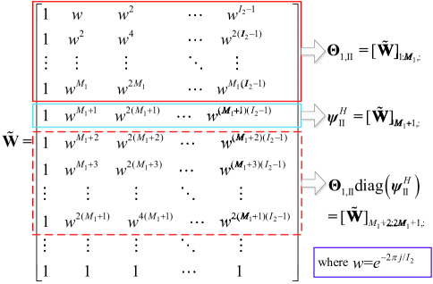
Figure 2: Illustration of constructing an optimal joint training design of ${\bm{\Theta}}_{1,\rm II}$ and ${\bm{\psi}}_{\rm II}$.

Let ${\bm{W}}$ denote the $I_{2}\times I_{2}$ DFT matrix, where $I_{2}\geq 2M_{1}+1$ is required for the LS estimation in (18). First, we move the first row of ${\bm{W}}$ to the last and form a new $I_{2}\times I_{2}$ matrix denoted by ${\tilde{\bm{W}}}$. To satisfy the conditions in (27)-(28), we let the training reflection matrix at IRS 1 as the first $M_{1}$ rows of ${\tilde{\bm{W}}}$, i.e., ${\bm{\Theta}}_{1,\rm II}=[{\tilde{\bm{W}}}]_{1:M_{1},:}$. Then it can be observed that, if we design the common phase-shift vector at IRS 2 as the $(M_{1}+1)$-th row of ${\tilde{\bm{W}}}$, i.e., ${\bm{\psi}}_{\rm II}^{H}=[{\tilde{\bm{W}}}]_{M_{1}+1,:}$, we then have ${\bm{\Theta}}_{1,\rm II}{\rm diag}({\bm{\psi}}_{\rm II}^{H})=[{\tilde{\bm{W}}}]_{M_{1}+2:2M_{1}+1,:}$ due to the row-shifting effect of ${\rm diag}({\bm{\psi}}_{\rm II}^{H})$ on ${\bm{\Theta}}_{1,\rm II}$ and thus the conditions in (29)-(30) can be simultaneously satisfied due to the pairwise orthogonality among rows in ${\tilde{\bm{W}}}$. The above optimal training reflection matrix construction is illustrated in Fig. 2. With the optimal ${\bm{\Theta}}_{1,\rm II}$ and ${\bm{\psi}}_{\rm II}$ that satisfy ${\bm{\Omega}}_{\rm II}{\bm{\Omega}}_{\rm II}^{H}=I_{2}{\bm{I}}_{2M_{1}+1}$, the minimum MSE of (III-B1) is achieved, which is given by $\varepsilon_{\rm II}^{\rm min}=\frac{\sigma^{2}}{I_{2}}$ for Phase II.

III-B2 Case 2

$N<M_{2}$. The MSE of the LS channel estimation in (23) is given by

$$\varepsilon_{\rm II}^{\prime} =\frac{1}{M_{2}+M_{1}M_{2}+NM_{1}}{\mathbb{E}}\left\{\left\|\begin{bmatrix}{\rm vec}({\hat{\bm{E}}})\\ {\rm vec}({\hat{\bm{R}}})\end{bmatrix}-\begin{bmatrix}{\rm vec}({{\bm{E}}})\\ {\rm vec}({{\bm{R}}})\end{bmatrix}\right\|^{2}\right\}$$

$$=\frac{1}{M_{2}+M_{1}M_{2}+NM_{1}}{\mathbb{E}}\left\{\Big{\|}{\bm{\Xi}}^{\dagger}{\bm{v}}_{\rm II}\Big{\|}^{2}\right\}$$

$$=\frac{1}{M_{2}+M_{1}M_{2}+NM_{1}}\text{tr}\left\{{\bm{\Xi}}^{\dagger}{\mathbb{E}}\left\{{\bm{v}}_{\rm II}{\bm{v}}_{\rm II}^{H}\right\}\left({\bm{\Xi}}^{\dagger}\right)^{H}\right\}$$

$$=\frac{\sigma^{2}}{M_{2}+M_{1}M_{2}+NM_{1}}\text{tr}\left\{\left({\bm{\Xi}}^{H}{\bm{\Xi}}\right)^{-1}\right\}$$ (31)

where ${\mathbb{E}}\left\{{\bm{v}}_{\rm II}{\bm{v}}_{\rm II}^{H}\right\}=\sigma^{2}{\bm{I}}_{I_{2}N}$. Moreover, according to the expression of ${\bm{\Xi}}$ given in (22), we have (III-B2) shown at the top of next page, where $(c)$ in (III-B2) is obtained according to the mixed-product property of Kronecker product.

$${\bm{\Xi}}^{H}{\bm{\Xi}}= \begin{bmatrix}({\tilde{\bm{\theta}}}_{1,\rm II}^{(1)})^{*}\otimes({\bar{\bm{Q}}}{\bm{\Psi}}_{\rm II}^{(1)})^{H}&\cdots&({\tilde{\bm{\theta}}}_{1,\rm II}^{(I_{2})})^{*}\otimes({\bar{\bm{Q}}}{\bm{\Psi}}_{\rm II}^{(I_{2})})^{H}\\ ({\bm{\theta}}_{1,\rm II}^{(1)})^{*}\otimes{\bm{I}}_{N}&\cdots&({\bm{\theta}}_{1,\rm II}^{(I_{2})})^{*}\otimes{\bm{I}}_{N}\end{bmatrix}\begin{bmatrix}({\tilde{\bm{\theta}}}_{1,\rm II}^{(1)})^{T}\otimes{\bar{\bm{Q}}}{\bm{\Psi}}_{\rm II}^{(1)}&({\bm{\theta}}_{1,\rm II}^{(1)})^{T}\otimes{\bm{I}}_{N}\\ \vdots&\vdots\\ ({\tilde{\bm{\theta}}}_{1,\rm II}^{(I_{2})})^{T}\otimes{\bar{\bm{Q}}}{\bm{\Psi}}_{\rm II}^{(I_{2})}&({\bm{\theta}}_{1,\rm II}^{(I_{2})})^{T}\otimes{\bm{I}}_{N}\end{bmatrix}$$

$$\stackrel{{\scriptstyle(c)}}{{=}} \sum_{i=1}^{I_{2}}\begin{bmatrix}\left(({\tilde{\bm{\theta}}}_{1,\rm II}^{(i)})^{*}({\tilde{\bm{\theta}}}_{1,\rm II}^{(i)})^{T}\right)\otimes\left(({\bar{\bm{Q}}}{\bm{\Psi}}_{\rm II}^{(i)})^{H}{\bar{\bm{Q}}}{\bm{\Psi}}_{\rm II}^{(i)}\right)&\left(({\tilde{\bm{\theta}}}_{1,\rm II}^{(i)})^{*}({\bm{\theta}}_{1,\rm II}^{(i)})^{T}\right)\otimes\left(({\bar{\bm{Q}}}{\bm{\Psi}}_{\rm II}^{(i)})^{H}\right)\\ \left(({\bm{\theta}}_{1,\rm II}^{(i)})^{*}({\tilde{\bm{\theta}}}_{1,\rm II}^{(i)})^{T}\right)\otimes\left({\bar{\bm{Q}}}{\bm{\Psi}}_{\rm II}^{(i)}\right)&\left(({\bm{\theta}}_{1,\rm II}^{(i)})^{*}({\bm{\theta}}_{1,\rm II}^{(i)})^{T}\right)\otimes{\bm{I}}_{N}\end{bmatrix}$$ (32)

It is noted that for any arbitrary ${\bar{\bm{Q}}}$ involved in (III-B2), it is generally difficult (if not impossible in some special cases) to jointly design the optimal training reflection phase-shifts $\left\{{\bm{\theta}}_{1,\rm II}^{(i)},{\bm{\theta}}_{2,\rm II}^{(i)}\right\}_{i=1}^{I_{2}}$ at the two IRSs in Phase II to minimize the MSE in (III-B2). Alternatively, we can construct the training reflection phase-shifts $\left\{{\bm{\theta}}_{1,\rm II}^{(i)},{\bm{\theta}}_{2,\rm II}^{(i)}\right\}_{i=1}^{I_{2}}$ based on some orthogonal matrices (e.g., the DFT matrix, Hadamard matrix, and circulant matrix generated by Zadoff-Chu sequence [39]) to achieve ${\rm rank}\left({\bm{\Xi}}\right)=M_{2}+M_{1}M_{2}+NM_{1}$ required by the LS estimation in (23).

IV Double-IRS Channel Estimation for Multi-User Case

For the multi-user channel estimation, a straightforward method is by adopting the single-user channel estimation in Section III to estimate the cascaded channels of $K$ users separately over consecutive time, which, however, increases the total training overhead by $K$ times as compared to the single-user case and thus is practically prohibitive if $K$ is large. To achieve more efficient channel training, we extend the proposed channel estimation scheme and training reflection design for the single-user case in Section III to the general multi-user case in this section in a different way. The key idea is to exploit the fact that given the cascaded channel of an arbitrary user (referred to as the reference user) estimated as in the single-user case (cf. Section III), the other users’ cascaded channels can be expressed as lower-dimensional scaled versions of it and thus estimated with substantially reduced channel training. The detailed channel estimation scheme and training reflection design for the general multi-user case are elaborated in the two subsequent subsections, respectively.

IV-A Extended Channel Estimation Scheme for Multiple Users

After estimating the cascaded channel of an arbitrary user as in the single-user case of Section III, the cascaded channels of the other users can be efficiently estimated by exploiting the property that all the users share the common IRS 2$\rightarrow$BS (i.e, ${{\bm{G}}}_{2}$), IRS 1$\rightarrow$BS (i.e, ${{\bm{G}}}_{1}$), and IRS 1$\rightarrow$IRS 2 (i.e, ${\bm{D}}$) links in their respective single- and double-reflection channels (see Fig. 1). In particular, we have the following lemma for the cascaded channels of the other users.

Lemma 2.

With the cascaded CSI of an arbitrary user (say, $\left\{{{\bm{Q}}}_{1,m}\right\}_{m=1}^{M_{1}}$, ${\tilde{\bm{R}}}_{1}$, and ${{\bm{R}}}_{1}$ of user 1) available as the reference CSI, we only need to estimate the scaling vectors ${{\bm{b}}}_{k}={\rm diag}\left({{\bm{u}}}_{1}\right)^{-1}{{\bm{u}}}_{k}\in{\mathbb{C}^{M_{1}\times 1}}$ and ${\tilde{\bm{b}}}_{k}={\rm diag}\left({\tilde{\bm{u}}}_{1}\right)^{-1}{\tilde{\bm{u}}}_{k}\in{\mathbb{C}^{M_{2}\times 1}}$ to acquire the cascaded CSI of the remaining $K-1$ users with $k=2,\ldots,K$.

Proof.

If given the cascaded CSI of user 1 as the reference CSI, we can rewrite the two single-reflection channels $\left\{{{\bm{R}}}_{k},{\tilde{\bm{R}}}_{k}\right\},\forall k=2,\ldots,K$ in (2) as

$${{\bm{R}}}_{k} ={{\bm{G}}}_{1}{\rm diag}\left({{\bm{u}}}_{k}\right)={{\bm{G}}}_{1}{\rm diag}\left({{\bm{u}}}_{1}\right)\cdot{\rm diag}\left({{\bm{u}}}_{1}\right)^{-1}{{\bm{u}}}_{k}$$

$$={{\bm{R}}}_{1}{\rm diag}\left({{\bm{b}}}_{k}\right)$$ (33)

$${\tilde{\bm{R}}}_{k} ={{\bm{G}}}_{2}{\rm diag}\left({\tilde{\bm{u}}}_{k}\right)={{\bm{G}}}_{2}{\rm diag}\left({\tilde{\bm{u}}}_{1}\right)\cdot{\rm diag}\left({\tilde{\bm{u}}}_{1}\right)^{-1}{\tilde{\bm{u}}}_{k}$$

$$={\tilde{\bm{R}}}_{1}{\rm diag}\left({\tilde{\bm{b}}}_{k}\right)$$ (34)

and the double-reflection channels $\left\{{{\bm{Q}}}_{k,m}\right\}_{m=1}^{M_{1}},\forall k=2,\ldots,K$ in (2) as

$${{\bm{Q}}}_{k,m}= {{\bm{G}}}_{2}{\rm diag}\left({\tilde{\bm{d}}}_{k,m}\right)={{\bm{G}}}_{2}{\rm diag}\left({\bm{d}}_{m}{{u}}_{k,m}\right)$$

$$= {{\bm{G}}}_{2}{\rm diag}\left({\bm{d}}_{m}{{u}}_{1,m}\right)\cdot{{u}}_{1,m}^{-1}{{u}}_{k,m}={{\bm{Q}}}_{1,m}{{b}}_{k,m}$$ (35)

with $m=1,\ldots,M_{1}$, where ${{\bm{b}}}_{k}\triangleq\left[{{b}}_{k,1},\ldots,{{b}}_{k,M_{1}}\right]^{T}={\rm diag}\left({{\bm{u}}}_{1}\right)^{-1}{{\bm{u}}}_{k}\in{\mathbb{C}^{M_{1}\times 1}}$ and ${\tilde{\bm{b}}}_{k}={\rm diag}\left({\tilde{\bm{u}}}_{1}\right)^{-1}{\tilde{\bm{u}}}_{k}\in{\mathbb{C}^{M_{2}\times 1}}$ are two scaling vectors of user $k$$\rightarrow$IRS 1 and user $k$$\rightarrow$IRS 2 channels normalized by ${{\bm{u}}}_{1}$ and ${\tilde{\bm{u}}}_{1}$, respectively. As such, with the cascaded CSI of user 1 available as the reference CSI, we only need to further estimate $\left\{{{\bm{b}}}_{k},{\tilde{\bm{b}}}_{k}\right\}_{k=2}^{K}$ to acquire the cascaded CSI of the remaining $K-1$ users according to the channel relationship in (33)-(IV-A), thus completing the proof. ∎

According to Lemma 2, after acquiring the cascaded CSI of user 1 as for the single-user case in Section III, we only need to further estimate the scaling vectors $\left\{{{\bm{b}}}_{k},{\tilde{\bm{b}}}_{k}\right\}_{k=2}^{K}$ for the remaining $K-1$ users. By substituting (33)-(IV-A) into (2), we can re-express the channel model in (2) as

$${\bm{h}}_{k}=\sum_{m=1}^{M_{1}}{{\bm{Q}}}_{1,m}{\bm{\theta}}_{2}{\theta}_{1,m}{{b}}_{k,m}+{\tilde{\bm{R}}}_{1}{\rm diag}\left({\tilde{\bm{b}}}_{k}\right){\bm{\theta}}_{2}+{{\bm{R}}}_{1}{\rm diag}\left({{\bm{b}}}_{k}\right){\bm{\theta}}_{1}$$

$$=\left[{{\bm{Q}}}_{1,1}{\bm{\theta}}_{2},\ldots,{{\bm{Q}}}_{1,M}{\bm{\theta}}_{2}\right]{\rm diag}\left({\bm{\theta}}_{1}\right){{\bm{b}}}_{k}$$

$$~{}~{}~{}+{\tilde{\bm{R}}}_{1}{\rm diag}\left({\bm{\theta}}_{2}\right){\tilde{\bm{b}}}_{k}+{{\bm{R}}}_{1}{\rm diag}\left({\bm{\theta}}_{1}\right){{\bm{b}}}_{k}$$

$$=\underbrace{\left[\left(\left[{{\bm{Q}}}_{1,1}{\bm{\theta}}_{2},\ldots,{{\bm{Q}}}_{1,M}{\bm{\theta}}_{2}\right]+{{\bm{R}}}_{1}\right){\bm{\Phi}}_{1},~{}{\tilde{\bm{R}}}_{1}{\bm{\Phi}}_{2}\right]}_{{\bm{B}}\in{\mathbb{C}^{N\times(M_{1}+M_{2})}}}\underbrace{\begin{bmatrix}{{\bm{b}}}_{k}\\ {\tilde{\bm{b}}}_{k}\end{bmatrix}}_{{\bm{\lambda}}_{k}}$$ (36)

where ${\bm{\lambda}}_{k}\in{\mathbb{C}^{(M_{1}+M_{2})\times 1}}$ denotes the the stacked scaling vector of user $k$. Following Phases I-II for estimating the cascaded CSI of the single user (i.e., user 1) in Section III, we propose the joint estimation of $\left\{{\bm{\lambda}}_{k}\right\}_{k=2}^{K}$ in the subsequent Phase III, which is elaborated in the next.

Phase III (Estimation of $\{{{\bm{b}}}_{k},{\tilde{\bm{b}}}_{k}\}_{k=2}^{K}$): In this phase, we fix the reflection phase-shifts of the two IRSs for simplicity, i.e., ${\bm{\theta}}_{1,\rm III}^{(i)}={\bm{\theta}}_{1,\rm III}$ and ${\bm{\theta}}_{2,\rm III}^{(i)}={\bm{\theta}}_{2,\rm III}$, and design the concurrent pilot symbols for the remaining $K-1$ users to facilitate the joint estimation of $\left\{{\bm{\lambda}}_{k}\right\}_{k=2}^{K}$. Based on the channel model in (36) with the fixed reflection phase-shifts $\left\{{\bm{\theta}}_{1,\rm III},{\bm{\theta}}_{2,\rm III}\right\}$ of the two IRSs, the received signal at the BS during symbol period $i$ of Phase III can be expressed as

$${\bm{z}}_{\rm III}^{(i)}=\sum_{k=2}^{K}x_{k}^{(i)}{\bm{B}}{\bm{\lambda}}_{k}+{\bm{v}}_{\rm III}^{(i)}={\bm{B}}\underbrace{\left[{\bm{\lambda}}_{2},\ldots,{\bm{\lambda}}_{K}\right]}_{{\bm{\Lambda}}}{\bm{x}}^{(i)}+{\bm{v}}_{\rm III}^{(i)}$$ (37)

where $i=1,\ldots,I_{3}$ with $I_{3}$ denoting the number of (pilot) symbol periods in Phase III, ${\bm{x}}^{(i)}=\left[x_{2}^{(i)},\ldots,x_{K}^{(i)}\right]^{T}\in{\mathbb{C}^{(K-1)\times 1}}$ denotes the pilot symbol vector transmitted by the remaining $K-1$ users, and ${\bm{v}}_{\rm III}^{(i)}\sim{\mathcal{N}_{c}}({\bm{0}},\sigma^{2}{\bm{I}}_{N})$ is the AWGN vector with normalized noise power of $\sigma^{2}$. Note that ${\bm{B}}$ can be regarded as the spatial observation matrix for (37) and its column rank will affect the training design and the corresponding minimum training overhead of Phase III. As such, for the joint estimation of ${\bm{\Lambda}}\triangleq\left[{\bm{\lambda}}_{2},\ldots,{\bm{\lambda}}_{K}\right]\in{\mathbb{C}^{(M_{1}+M_{2})\times(K-1)}}$, we consider the following two cases depending on whether ${\bm{B}}$ is of full column rank or not.

IV-A1 Case 1

$N\geq M_{1}+M_{2}$. In this case, we stack the received signal vectors $\left\{{\bm{z}}_{\rm III}^{(i)}\right\}$ over $I_{3}$ symbol periods as ${\bm{Z}}_{\rm III}=\left[{\bm{z}}_{\rm III}^{(1)},{\bm{z}}_{\rm III}^{(2)},\ldots,{\bm{z}}_{\rm III}^{(I_{3})}\right]\in{\mathbb{C}^{N\times I_{3}}}$ and thus obtain

$${\bm{Z}}_{\rm III} ={\bm{B}}{\bm{\Lambda}}{\bm{X}}+{\bm{V}}_{\rm III}$$ (38)

where ${\bm{X}}=\left[{\bm{x}}^{(1)},{\bm{x}}^{(2)},\ldots,{\bm{x}}^{(I_{3})}\right]\in{\mathbb{C}^{(K-1)\times I_{3}}}$ is the pilot symbol matrix of the remaining $K-1$ users and ${\bm{V}}_{\rm III}=\left[{\bm{v}}_{\rm III}^{(1)},{\bm{v}}_{\rm III}^{(2)},\ldots,{\bm{v}}_{\rm III}^{(I_{3})}\right]\in{\mathbb{C}^{N\times I_{3}}}$ is the corresponding AWGN matrix. By properly designing the training reflection phase-shifts $\left\{{\bm{\theta}}_{1,\rm III},{\bm{\theta}}_{2,\rm III}\right\}$ of the two IRSs as well as the pilot symbol matrix ${\bm{X}}$ such that ${\rm rank}\left({\bm{B}}\right)=M_{1}+M_{2}$ and ${\rm rank}\left({\bm{X}}\right)=K-1$, the LS estimate of ${\bm{\Lambda}}$ based on (38) is given by

$${\hat{\bm{\Lambda}}}={\bm{B}}^{\dagger}{\bm{Z}}_{\rm III}{\bm{X}}^{\dagger}={\bm{\Lambda}}+{\bm{B}}^{\dagger}{\bm{V}}_{\rm III}{\bm{X}}^{\dagger}$$ (39)

where ${\bm{B}}^{\dagger}=\left({\bm{B}}^{H}{\bm{B}}\right)^{-1}{\bm{B}}^{H}$ and ${\bm{X}}^{\dagger}={\bm{X}}^{H}\left({\bm{X}}{\bm{X}}^{H}\right)^{-1}$. Note that $I_{3}\geq K-1$ is required to ensure ${\rm rank}\left({\bm{X}}\right)=K-1$ and thus the existence of ${\bm{X}}^{\dagger}$ for the case of $N\geq M_{1}+M_{2}$.

IV-A2 Case 2

$N<M_{1}+M_{2}$. In this case, since ${\bm{B}}$ is (column) rank-deficient, i.e., ${\rm rank}\left({\bm{B}}\right)=N<M_{1}+M_{2}$, we cannot estimate ${\bm{\Lambda}}$ according to (39). Alternatively, we stack the received signal vectors $\{{\bm{z}}_{\rm III}^{(i)}\}$ over $I_{3}$ symbol periods as ${\bm{z}}_{\rm III}=\left[({\bm{z}}_{\rm III}^{(1)})^{T},({\bm{z}}_{\rm III}^{(2)})^{T},\ldots,({\bm{z}}_{\rm III}^{(I_{3})})^{T}\right]^{T}={\rm vec}\left({\bm{Z}}_{\rm III}\right)\in{\mathbb{C}^{I_{3}N\times 1}}$ and thus obtain

$${\bm{z}}_{\rm III}=\left({\bm{X}}^{T}\otimes{\bm{B}}\right){\rm vec}\left({\bm{\Lambda}}\right)+{\bm{v}}_{\rm III}$$ (40)

where ${\bm{v}}_{\rm III}=\left[({\bm{v}}_{\rm III}^{(1)})^{T},({\bm{v}}_{\rm III}^{(2)})^{T},\ldots,({\bm{v}}_{\rm III}^{(I_{3})})^{T}\right]^{T}\in{\mathbb{C}^{I_{3}N\times 1}}$ is the corresponding AWGN vector in Phase III. Accordingly, if we design the training reflection phase-shifts $\left\{{\bm{\theta}}_{1,\rm III},{\bm{\theta}}_{2,\rm III}\right\}$ of the two IRSs as well as the pilot symbol matrix ${\bm{X}}$ properly such that ${\rm rank}\left({\bm{X}}^{T}\otimes{\bm{B}}\right)=(K-1)(M_{1}+M_{2})$, the LS estimate of ${\rm vec}\left({\bm{\Lambda}}\right)$ based on (40) is given by

$${\rm vec}\left({\hat{\bm{\Lambda}}}\right)=\left({\bm{X}}^{T}\otimes{\bm{B}}\right)^{\dagger}{\bm{z}}_{\rm III}={\rm vec}\left({\bm{\Lambda}}\right)+\left({\bm{X}}^{T}\otimes{\bm{B}}\right)^{\dagger}{\bm{v}}_{\rm III}$$ (41)

where $\left({\bm{X}}^{T}\otimes{\bm{B}}\right)^{\dagger}=\left(\left({\bm{X}}^{T}\otimes{\bm{B}}\right)^{H}\left({\bm{X}}^{T}\otimes{\bm{B}}\right)\right)^{-1}\left({\bm{X}}^{T}\otimes{\bm{B}}\right)^{H}$. Note that since $I_{3}N\geq(K-1)(M_{1}+M_{2})$ is required to ensure ${\rm rank}\left({\bm{X}}^{T}\otimes{\bm{B}}\right)=(K-1)(M_{1}+M_{2})$ with $I_{3}$ being an integer, we have $I_{3}\geq\left\lceil\frac{(K-1)(M_{1}+M_{2})}{N}\right\rceil$ for the case of $N<M_{1}+M_{2}$. Moreover, it is worth pointing out that the LS channel estimation based on (41) for the case of $N<M_{1}+M_{2}$ can also be applied to the case of $N\geq M_{1}+M_{2}$, but it incurs higher complexity due to the larger-size matrix inversion operation for $\left({\bm{X}}^{T}\otimes{\bm{B}}\right)^{\dagger}$.

IV-B Training Design for Multiple Users

It can be verified that for the case of $N\geq M_{1}+M_{2}$, the LS channel estimation based on (41) is also equivalent to that based on (39) with proper vectorization. As such, we focus on the MSE derivation for the LS channel estimation based on (41), which is given by

$$\varepsilon_{\rm III}=\frac{1}{(K-1)(M_{1}+M_{2})}{\mathbb{E}}\left\{\left\|{\rm vec}\left({\hat{\bm{\Lambda}}}\right)-{\rm vec}\left({\bm{\Lambda}}\right)\right\|^{2}\right\}$$

$$=\frac{1}{(K-1)(M_{1}+M_{2})}{\mathbb{E}}\left\{\Big{\|}\left({\bm{X}}^{T}\otimes{\bm{B}}\right)^{\dagger}{\bm{v}}_{\rm III}\Big{\|}^{2}\right\}$$

$$=\frac{1}{(K-1)(M_{1}+M_{2})}\text{tr}\left\{\left({\bm{X}}^{T}\otimes{\bm{B}}\right)^{\dagger}{\mathbb{E}}\left\{{\bm{v}}_{\rm III}{\bm{v}}_{\rm III}^{H}\right\}\left(\left({\bm{X}}^{T}\otimes{\bm{B}}\right)^{\dagger}\right)^{H}\right\}$$

$$=\frac{\sigma^{2}}{(K-1)(M_{1}+M_{2})}\text{tr}\left\{\left(\left({\bm{X}}^{T}\otimes{\bm{B}}\right)^{H}\left({\bm{X}}^{T}\otimes{\bm{B}}\right)\right)^{-1}\right\}$$

$$\stackrel{{\scriptstyle(d)}}{{=}}\frac{\sigma^{2}}{(K-1)(M_{1}+M_{2})}\text{tr}\left\{\left({\bm{X}}{\bm{X}}^{H}\right)^{-1}\right\}\text{tr}\left\{\left({\bm{B}}^{H}{\bm{B}}\right)^{-1}\right\}$$ (42)

where ${\mathbb{E}}\left\{{\bm{v}}_{\rm III}{\bm{v}}_{\rm III}^{H}\right\}=\sigma^{2}{\bm{I}}_{I_{3}N}$ and $(d)$ is obtained according to the mixed-product and trace properties of Kronecker product. As such, the MSE minimization in (IV-B) is equivalent to minimizing $\text{tr}\left\{\left({\bm{X}}{\bm{X}}^{H}\right)^{-1}\right\}$ and $\text{tr}\left\{\left({\bm{B}}^{H}{\bm{B}}\right)^{-1}\right\}$, respectively. Specifically, the minimization of $\text{tr}\left\{\left({\bm{X}}{\bm{X}}^{H}\right)^{-1}\right\}$ can be achieved if and only if ${\bm{X}}{\bm{X}}^{H}=I_{3}{\bm{I}}_{K-1}$, which implies that the pilot sequences from the remaining $K-1$ users should be orthogonal to each other in Phase III. Accordingly, we can design the pilot symbol matrix ${\bm{X}}$ in Phase III as e.g., the submartix of the $I_{3}\times I_{3}$ DFT matrix with its first $K-1$ rows. On the other hand, since the matrix ${\bm{B}}$ involves the cascaded CSI of $\left\{{{\bm{Q}}}_{1,m}\right\}_{m=1}^{M_{1}}$, ${\tilde{\bm{R}}}_{1}$, and ${{\bm{R}}}_{1}$ which can be arbitrary in practice, it is generally difficult to design the optimal training reflection phase-shifts of the two IRSs to minimize $\text{tr}\left\{\left({\bm{B}}^{H}{\bm{B}}\right)^{-1}\right\}$. Alternatively, we can design the training reflection phase-shifts of the two IRSs based on some orthogonal matrices/sequences (e.g., the DFT matrix), to satisfy the rank conditions required by the LS channel estimations in (39) and (41), whose performance will be examined by simulations in Section V.

V Numerical Results

In this section, we present numerical results to validate the effectiveness of our proposed channel estimation scheme as well as the corresponding training design for the double-IRS aided multi-user MIMO system. Under the three-dimensional (3D) Cartesian coordinate system, we assume that the central (reference) points of the BS, IRS 2, IRS 1, and user cluster are located at $(1,0,2)$, $(0,0.5,1)$, $(0,49.5,1)$, and $(1,50,0)$ in meter (m), respectively. Moreover, we assume that the BS is equipped with a uniform linear array (ULA); while the two distributed IRSs are equipped with uniform planar arrays (UPAs). As the element-grouping strategy adopted in [37, 27], each IRS subsurface is a small-size UPA composed of $5\times 5$ adjacent reflecting elements that share a common phase shift for reducing design complexity. The distance-dependent channel path loss is modeled as $\gamma=\gamma_{0}/d^{\alpha}$, where $\gamma_{0}$ denotes the path loss at the reference distance of 1 m which is set as $\gamma_{0}=-30$ dB for all individual links, $d$ denotes the individual link distance, and $\alpha$ denotes the path loss exponent which is set as $2.2$ for the link between the user cluster/BS and its nearby serving IRS (due to the short distance) and set as $3$ for the other links (due to the relatively longer distances). Without loss of generality, all the users are assumed to have equal transmit power, i.e., $P_{k}=P,\forall k=1,\ldots,K$ and the noise power at the BS is set as $\sigma^{2}_{N}=-65$ dBm. Accordingly, the normalized noise power at the BS is given by $\sigma^{2}=\sigma^{2}_{N}/P$.

Note that there has been very limited work on channel estimation for the double-IRS aided system with the co-existence of single- and double-reflection links. As such, we consider the following two benchmark channel estimation schemes for comparison.

• Decoupled scheme with ON/OFF IRSs [1]: For the single-user case of this scheme, the cascaded channels of the two single-reflection links, each corresponding to one of the two IRSs respectively, are successively estimated at the multi-antenna BS with the other IRS turned OFF. Then, after canceling the signals over the two single-reflection channels estimated, the higher-dimensional double-reflection (i.e., user$\rightarrow$IRS 1$\rightarrow$IRS 2$\rightarrow$BS) channel is efficiently estimated at the BS by exploiting the fact that its cascaded channel coefficients are scaled versions of those of the single-reflection (i.e., user$\rightarrow$IRS 2$\rightarrow$BS) channel due to their commonly shared IRS 2$\rightarrow$BS link. For the multi-user case, by leveraging the same (common) channel relationship among users in Lemma 2, the scaling vectors $\left\{{{\bm{b}}}_{k}\right\}_{k=2}^{K}$ and $\left\{{\tilde{\bm{b}}}_{k}\right\}_{k=2}^{K}$ are separately estimated at the BS with one of the two IRSs turned OFF.

• Benchmark scheme based on [26]: We extend the channel estimation method proposed in [26] as another benchmark scheme, where the double-reflection channel is estimated at each BS antenna in parallel without exploiting the (common) channel relationship with the single-reflection channels, and the cascaded channels of $K$ users are separately estimated over consecutive time. Moreover, as the single-reflection channels were ignored in [26], the same decoupled channel estimation for the two single-reflection channels in [1] is adopted for each user in this benchmark scheme.

V-A Training Overhead Comparison

The training overhead comparison between the proposed channel estimation scheme and the two benchmark schemes is shown in Table I, where $M_{1}=M_{2}=M/2$ is assumed for ease of exposition. As can be seen in Table I, by exploiting the peculiar channel relationship over single- and double-reflection channels as well as that among multiple users, both the proposed channel estimation scheme with always-ON IRSs and the decoupled channel estimation scheme with ON/OFF IRSs incur much lower-order training overhead than the benchmark scheme based on [26], especially when $N\geq M$. In the rest of this section, given the total number of subsurfaces $M=40$, we set $M_{1}=M_{2}=M/2=20$ for the two distributed IRSs.

TABLE I: Training Overhead Comparison for Different Channel Estimation Schemes (Assume $M_{1}=M_{2}=M/2$)

	Minimum number of (pilot) symbol periods
	$N\geq M$	$M>N\geq M/2$	$N<M/2$
Proposed scheme with always-ON IRSs	$\frac{3}{2}M+K+1$	$\frac{3}{2}M+2+\left\lceil\frac{(K-1)M}{N}\right\rceil$	$M+1+\left\lceil\frac{(M+2)M}{4N}\right\rceil+\left\lceil\frac{(K-1)M}{N}\right\rceil$
Decoupled scheme with ON/OFF IRSs [1]	$\frac{3}{2}M+2(K-1)$		$M+\left\lceil\frac{M^{2}}{4N}\right\rceil+2\left\lceil\frac{(K-1)M}{2N}\right\rceil$
Benchmark scheme based on [26]	$KM+\frac{1}{4}KM^{2}$

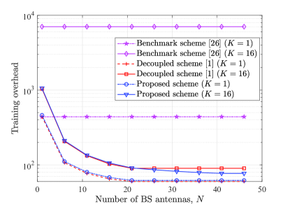
(a) Training overhead versus number of BS antennas $N$.

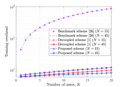
(b) Training overhead versus number of users $K$.

Figure 3: Training overhead comparison of different channel estimation schemes.

In Fig. 3(a), we show the required training overhead versus the number of BS antennas $N$. It is observed that for both the proposed and decoupled channel estimation schemes, their training overheads decrease dramatically with the increasing number of BS antennas $N$, which is in sharp contrast to the benchmark scheme based on [26] where its training overhead is independent of $N$. This is expected since both the proposed and decoupled channel estimation schemes exploit the (common) channel relationship and the multiple antennas at the BS for joint cascaded channel estimation to reduce their training overheads substantially; whereas in the benchmark scheme based on [26], the BS estimates its cascaded channels associated with different antennas/users independently in parallel without exploiting the channel relationship between them. When the number of BS antennas is sufficiently large (i.e., $N\geq M=40$), the required training overheads of the proposed and decoupled channel estimation schemes reach their respective lower bounds of $\frac{3}{2}M+K+1$ and $\frac{3}{2}M+2(K-1)$ pilot symbols, as given in Table I.

In Fig. 3(b), we show the required training overhead versus the number of users $K$. One can observe that the training overhead increment is marginal in both the proposed and decoupled channel estimation schemes as the number of users $K$ increases. In contrast, the training overhead required by the benchmark scheme based on [26] increases dramatically with $K$ since it estimates the channels of different users separately over consecutive time. In particular, the additional training overhead with one more user is $\text{max}\{1,\left\lceil\frac{M}{N}\right\rceil\}$ and $\text{max}\{2,2\left\lceil\frac{M}{2N}\right\rceil\}$ for the proposed and decoupled channel estimation schemes, respectively; whereas that for the benchmark scheme based on [26] is $M+\frac{1}{4}M^{2}$, which is considerably higher when $M$ is large.

V-B Normalized MSE Comparison for Single-User Case

In the following simulations, we calculate the normalized MSE for different channels estimated over $1,000$ independent fading channel realizations. For example, the normalized MSE of the cascaded user$\rightarrow$IRS 1$\rightarrow$BS channel ${{\bm{R}}}$ estimated is given by

$${\varepsilon}_{{\bm{R}}}=\frac{1}{NM_{1}}{\mathbb{E}}\left\{\left\|{\hat{\bm{R}}}-{{\bm{R}}}\right\|^{2}_{F}\Big{/}{\left\|{{\bm{R}}}\right\|^{2}_{F}}\right\}.$$ (43)

The normalized MSE of other channels estimated can be similarly calculated as the above.

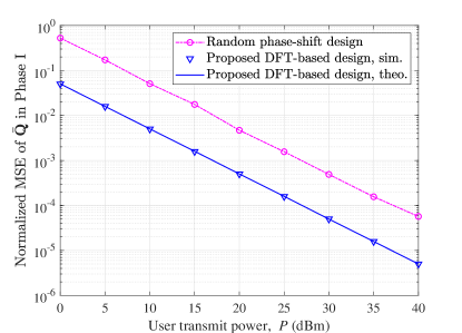
(a) Normalized MSE of ${\bar{\bm{Q}}}$ in Phase I versus user transmit power $P$.

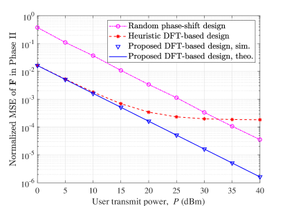
(b) Normalized MSE of ${{\bm{F}}}$ in Phase II versus user transmit power $P$.

Figure 4: Normalized MSE comparison of different training reflection designs for the single-user case with $N=25$.

We first compare different training reflection designs of the proposed channel estimation scheme under the single-user setup with $N=25$. In Figs. 4(a) and 4(b), we show the normalized MSE versus user transmit power $P$ for different training reflection designs in Phases I and II, respectively. It is observed that the theoretical (theo.) analysis of MSE given in Section 4 is in perfect agreement with the simulation (sim.) results for our proposed optimal training design in the two Phases. For Phase I shown in Fig. 4(a), the proposed DFT-based design achieves up to $10$ dB power gain over the random phase-shift design where the training reflection phase-shifts of ${\bar{\bm{\Theta}}}_{2,\rm I}$ are randomly generated following the uniform distribution within $[0,2\pi)$. For Phase II shown in Fig. 4(b), the joint training reflection design of the two IRSs is more involved and we consider the heuristic DFT-based design with ${\bm{\Theta}}_{1,\rm II}$ and ${\bm{\psi}}_{\rm II}$ drawn from the first (or any randomly selected) $M_{1}+1$ rows of the $I_{2}\times I_{2}$ DFT matrix as another benchmark design for comparison. It is observed from Fig. 4(b) that by carefully choosing $M_{1}+1$ rows from the DFT matrix to ensure the perfect orthogonality of ${\bm{\Omega}}_{\rm II}$ with the joint training reflection design of ${\bm{\Theta}}_{1,\rm II}$ and ${\bm{\psi}}_{\rm II}$, our proposed DFT-based design achieves much lower MSE than the heuristic DFT-based design as well as the random phase-shift design.

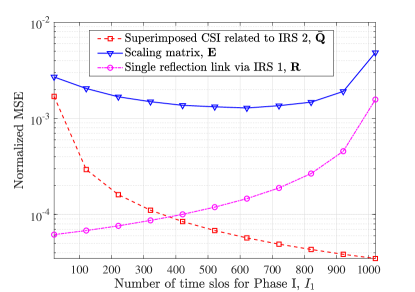
(a) Normalized MSE versus number of pilot symbols allocated to Phase I for estimating $\left\{{\bar{\bm{Q}}},{{\bm{E}}},{{\bm{R}}}\right\}$ in (9) of Lemma 1.

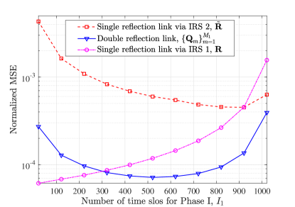
(b) Normalized MSE versus number of pilot symbols allocated to Phase I for estimating $\left\{\left\{{{\bm{Q}}}_{m}\right\}_{m=1}^{M_{1}},{\tilde{\bm{R}}},{{\bm{R}}}\right\}$ in (2).

Figure 5: Normalized MSE versus number of pilot symbols allocated to Phase I for the single-user case, where the total number of pilot symbols over the two phases is fixed as $I_{1}+I_{2}=1062$, $P=15$ dBm, and $N=25$.

In Fig. 5, we show the normalized MSE versus the number of pilot symbols allocated to Phase I, $I_{1}$, for estimating different CSI required for the channel models in (9) and (2), respectively, where the total number of pilot symbols over the two training phases is fixed as $I_{1}+I_{2}=1062$ for the single-user case. It is observed from Fig. 5 that the MSE of $\left\{{{\bm{E}}},\left\{{{\bm{Q}}}_{m}\right\}_{m=1}^{M_{1}},{\tilde{\bm{R}}}\right\}$ first decreases and then increases with the increasing number of pilot symbols allocated to Phase I. This is expected since the channel estimation error of Phase I will affect the channel estimation performance of Phase II due to the channel estimation error propagation. Intuitively, for the estimation of $\left\{{{\bm{E}}},\left\{{{\bm{Q}}}_{m}\right\}_{m=1}^{M_{1}},{\tilde{\bm{R}}}\right\}$, if more pilot symbols are allocated to Phase I, the error propagation effect to Phase II will be reduced, while less time is left for channel estimation in Phase II given the fixed overall training overhead. In contrast, as the CSI ${\bar{\bm{Q}}}$ (${{\bm{R}}}$) is estimated in Phase I (Phase II) only without suffering from the error propagation issue, the corresponding MSE thus monotonically decreases (increases) with the increasing number of pilot symbols allocated to Phase I given the fixed overall training overhead.

As shown in Fig. 3, the benchmark scheme based on [26] is much less efficient due to its higher-order training overhead. Moreover, it was shown in [1] that given the same training overhead, the decoupled channel estimation scheme with ON/OFF IRSs already achieves much better performance than the benchmark scheme based on [26] in terms of normalized MSE. As such, we mainly focus on the normalized MSE comparison between the proposed and decoupled channel estimation schemes in Fig. 6, considering their comparable minimum training overheads shown in Table I with $K=1$.

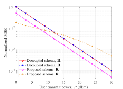
(a) Normalized MSE versus user transmit power $P$ for estimating the CSI of the two single-reflection links $\left\{{\tilde{\bm{R}}},{{\bm{R}}}\right\}$.

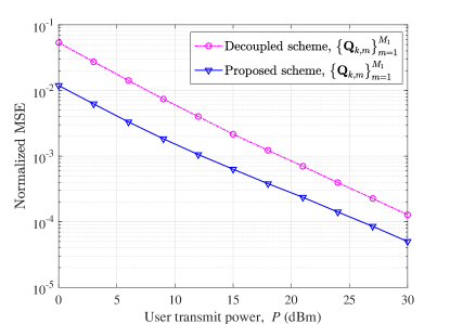
(b) Normalized MSE versus user transmit power $P$ for estimating the CSI of the double-reflection link $\left\{{{\bm{Q}}}_{m}\right\}_{m=1}^{M_{1}}$.

Figure 6: Normalized MSE comparison of different channel estimation schemes with $N=25$.

In Fig. 6(a), we compare the normalized MSE of the proposed and decoupled channel estimation schemes versus user transmit power $P$ for estimating the cascaded CSI of the two single-reflection links $\left\{{\tilde{\bm{R}}},{{\bm{R}}}\right\}$. It is observed that the proposed channel estimation scheme has different (asymmetric) normalized MSE performance for estimating the cascaded CSI of the two single-reflection links. This can be understood by the fact that the estimation of ${\tilde{\bm{R}}}$ is affected by the error propagation from Phase I to Phase II; while the estimation of ${{\bm{R}}}$ involves Phase II only without suffering from the error propagation issue, as discussed for Fig. 5. In contrast, the decoupled channel estimation scheme has the same (symmetric) normalized MSE performance for estimating the cascaded CSI of the two single-reflection links, which is due to the successive/separate channel estimation of $\left\{{\tilde{\bm{R}}},{{\bm{R}}}\right\}$ with equal training time. Two interesting observations are also made as follows in comparing the performance of the proposed and decoupled channel estimation schemes. First, by exploiting the full-reflection power of the two IRSs for estimating ${{\bm{R}}}$, the proposed channel estimation scheme with always-ON IRSs achieves up to 3 dB power gain over the decoupled counterpart with only one of the two IRSs turned ON successively over training. Second, the proposed channel estimation scheme is observed to achieve lower normalized MSE when $P\leq 12$ dBm while higher normalized MSE when $P>12$ dBm for estimating ${\tilde{\bm{R}}}$, as compared to the decoupled scheme. This is because the normalized MSE performance of the proposed channel estimation scheme for estimating ${\tilde{\bm{R}}}$ is limited by the error propagation in the two phases, thus suffering from a lower deceasing rate of the normalized MSE as user transmit power $P$ increases.

In Fig. 6(b), we compare the normalized MSE of the proposed and decoupled channel estimation schemes versus user transmit power $P$ for estimating the cascaded CSI of the double-reflection links $\left\{{{\bm{Q}}}_{m}\right\}_{m=1}^{M_{1}}$. As discussed in Fig. 5, the estimation of $\left\{{{\bm{Q}}}_{m}\right\}_{m=1}^{M_{1}}$ is affected by the error propagation from Phase I to Phase II in the proposed scheme. On the other hand, with the signals canceled over the two single-reflection channels estimated and the estimated ${\tilde{\bm{R}}}$ taken as the reference CSI, the decoupled channel estimation scheme encounters not only the error propagation issue but also the residual interference due to imperfect signal cancellation for estimating $\left\{{{\bm{Q}}}_{m}\right\}_{m=1}^{M_{1}}$, thus resulting in higher normalized MSE than the proposed scheme.

V-C Normalized MSE Comparison for Multi-User Case

Last, we compare the normalized MSE performance between the proposed and decoupled channel estimation schemes for the multi-user case with $K=10$ in Fig. 7, considering their comparable minimum training overheads as shown in Fig. 3(b). Note that both the proposed and decoupled channel estimation schemes reduce the training overhead for the multi-user case by exploiting the fact that the other users’ cascaded channels are lower-dimensional scaled versions of an arbitrary (reference) user’s cascaded channel; as a result, both the two schemes only need to estimate the scaling vectors $\left\{{{\bm{b}}}_{k},{\tilde{\bm{b}}}_{k}\right\}_{k=2}^{K}$, with user 1 taken as the reference user. For the decoupled channel estimation scheme, the scaling vectors $\left\{{{\bm{b}}}_{k}\right\}_{k=2}^{K}$ and $\left\{{\tilde{\bm{b}}}_{k}\right\}_{k=2}^{K}$ are successively estimated at the BS with one of the two IRSs turned OFF; while for the proposed channel estimation scheme, $\left\{{{\bm{b}}}_{k},{\tilde{\bm{b}}}_{k}\right\}_{k=2}^{K}$ are jointly estimated at the BS with always-ON IRSs.

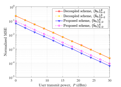
(a) Normalized MSE versus user transmit power $P$ for estimating the scaling vectors $\left\{{{\bm{b}}}_{k},{\tilde{\bm{b}}}_{k}\right\}_{k=2}^{K}$.

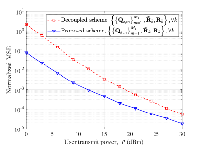
(b) Normalized MSE versus user transmit power $P$ for estimating the cascaded CSI of all users.

Figure 7: Normalized MSE comparison of different channel estimation schemes with $N=45$ and $K=10$.

In Fig. 7(a), we show the normalized MSE of the scaling vectors $\left\{{{\bm{b}}}_{k},{\tilde{\bm{b}}}_{k}\right\}_{k=2}^{K}$ by the proposed and decoupled channel estimation schemes versus user transmit power $P$ under the multi-user setup, where the cascaded CSI of user 1 (i.e., $\left\{{{\bm{Q}}}_{1,m}\right\}_{m=1}^{M_{1}}$, ${\tilde{\bm{R}}}_{1}$, and ${{\bm{R}}}_{1}$) is assumed to be perfectly available as the reference CSI for ease of comparison. Some important observations are made as follows. First, with the always-ON IRSs for maximizing the signal reflection power, the proposed channel estimation scheme achieves much better performance than the decoupled scheme with the ON/OFF IRS reflection design, in terms of the normalized MSE of $\left\{{{\bm{b}}}_{k}\right\}_{k=2}^{K}$ and $\left\{{\tilde{\bm{b}}}_{k}\right\}_{k=2}^{K}$. Second, the proposed channel estimation scheme has different (asymmetric) normalized MSE performance for estimating $\left\{{{\bm{b}}}_{k}\right\}_{k=2}^{K}$ and $\left\{{\tilde{\bm{b}}}_{k}\right\}_{k=2}^{K}$. This can be understood from (33)-(IV-A) that each ${{\bm{b}}}_{k}$ is associated with both the single-reflection (i.e., user $k$$\rightarrow$IRS 1$\rightarrow$BS) channel and the double-reflection (i.e., user $k$$\rightarrow$IRS 1$\rightarrow$IRS 2$\rightarrow$BS) channel, thus reaping higher reflection power for channel estimation than each ${\tilde{\bm{b}}}_{k}$ that is associated with the single-reflection (i.e., user $k$$\rightarrow$IRS 2$\rightarrow$BS) channel only. On the other hand, the decoupled channel estimation scheme has the same (symmetric) normalized MSE performance for estimating $\left\{{{\bm{b}}}_{k}\right\}_{k=2}^{K}$ and $\left\{{\tilde{\bm{b}}}_{k}\right\}_{k=2}^{K}$, which is due to the successive/separate channel estimation of them with nearly equal training time and single-reflection power.

In Fig. 7(b), we show the normalized MSE of the proposed and decoupled channel estimation schemes versus user transmit power $P$ accounting for all the cascaded CSI (i.e., $\left\{\left\{{{\bm{Q}}}_{k,m}\right\}_{m=1}^{M_{1}},{\tilde{\bm{R}}}_{k},{{\bm{R}}}_{k}\right\},\forall k$) under the multi-user case. It is observed that the proposed channel estimation scheme outperforms the decoupled counterpart significantly. This is expected due to the cumulative superior performance of the proposed channel estimation scheme as shown in Figs. 6 and 7(a).

VI Conclusions and Future Directions

In this paper, we proposed an efficient uplink channel estimation scheme for the double-IRS aided multi-user MIMO system with both IRSs always turned ON during the entire channel training for maximizing their reflected signal power. For the single-user case, minimum training time is achieved by exploiting the fact that the cascaded CSI of the single- and double-reflection links related to IRS 2 is lower-dimensional scaled versions of their superimposed CSI. For the multi-user case, by further exploiting the fact that all other users’ cascaded channels are also lower-dimensional scaled versions of an arbitrary (reference) user’s cascaded channel (estimated as in the single-user case), the multi-user cascaded channels are estimated with minimum training overhead. Moreover, for the proposed channel estimation scheme, we designed the corresponding training reflection phase-shifts for the double IRSs to minimize the channel estimation error over different training phases. In addition, we showed an interesting trade-off of training time allocation over different training phases with their intricate error propagation effect taken into account. Simulation results demonstrated the effectiveness of the proposed channel estimation scheme and training reflection phase-shift design, as compared to the existing channel estimation schemes and other heuristic training designs.

In the future, it is an interesting direction to study the more general multi-IRS aided multi-user communication system with multi-hop signal reflection [40, 38], which calls for more technically challenging system designs on channel estimation, joint passive beamforming, and multi-IRS deployment. Moreover, besides the CSI-based (robust) beamforming design, the beam training [31] and machine learning [41] based methods (that do not require the CSI explicitly) are also promising solutions to the multi-IRS aided multi-user communication system, which deserve more investigation in the future.

Beixiong Zheng (M’18) received the B.S. and Ph.D. degrees from the South China University of Technology, Guangzhou, China, in 2013 and 2018, respectively. He is currently a Research Fellow with the Department of Electrical and Computer Engineering, National University of Singapore. His recent research interests include intelligent reflecting surface (IRS), index modulation (IM), and non-orthogonal multiple access (NOMA). From 2015 to 2016, he was a Visiting Student Research Collaborator with Columbia University, New York, NY, USA. He was a recipient of the Best Paper Award from the IEEE International Conference on Computing, Networking and Communications in 2016, the Best Ph.D. Thesis Award from China Education Society of Electronics in 2018, the Exemplary Reviewer of the IEEE TRANSACTIONS ON COMMUNICATIONS, and the Outstanding Reviewer of Physical Communication.

Changsheng You (M’19) received his B.Eng. degree in 2014 from University of Science and Technology of China in electronic engineering and information science, and Ph.D. degree in 2018 from The University of Hong Kong in electrical and electronic engineering. He is currently a Research Fellow with the Department of Electrical and Computer Engineering, National University of Singapore. He is an editor for IEEE COMMUNICATIONS LETTERS. His research interests include intelligent reflecting surface, UAV communications, edge learning, mobile-edge computing, wireless power transfer, and convex optimization. Dr. You received the IEEE Communications Society Asia-Pacific Region Outstanding Paper Award in 2019 and the Exemplary Reviewer of the IEEE TRANSACTIONS ON COMMUNICATIONS and IEEE TRANSACTIONS ON WIRELESS COMMUNICATIONS. He was a recipient of the Best Ph.D. Thesis Award of The University of Hong Kong in 2019.

Rui Zhang (S’00-M’07-SM’15-F’17) received the B.Eng. (first-class Hons.) and M.Eng. degrees from the National University of Singapore, Singapore, and the Ph.D. degree from the Stanford University, Stanford, CA, USA, all in electrical engineering. From 2007 to 2010, he worked at the Institute for Infocomm Research, ASTAR, Singapore. Since 2010, he has been working with the National University of Singapore, where he is now a Professor in the Department of Electrical and Computer Engineering. He has published over 200 journal papers and over 180 conference papers. He has been listed as a Highly Cited Researcher by Thomson Reuters/Clarivate Analytics since 2015. His current research interests include UAV/satellite communications, wireless power transfer, reconfigurable MIMO, and optimization methods. He was the recipient of the 6th IEEE Communications Society Asia-Pacific Region Best Young Researcher Award in 2011, the Young Researcher Award of National University of Singapore in 2015, and the Wireless Communications Technical Committee Recognition Award in 2020. He was the co-recipient of the IEEE Marconi Prize Paper Award in Wireless Communications in 2015 and 2020, the IEEE Communications Society Asia-Pacific Region Best Paper Award in 2016, the IEEE Signal Processing Society Best Paper Award in 2016, the IEEE Communications Society Heinrich Hertz Prize Paper Award in 2017 and 2020, the IEEE Signal Processing Society Donald G. Fink Overview Paper Award in 2017, and the IEEE Technical Committee on Green Communications & Computing (TCGCC) Best Journal Paper Award in 2017. His co-authored paper received the IEEE Signal Processing Society Young Author Best Paper Award in 2017. He served for over 30 international conferences as the TPC co-chair or an organizing committee member, and as the guest editor for 3 special issues in the IEEE JOURNAL OF SELECTED TOPICS IN SIGNAL PROCESSING and the IEEE JOURNAL ON SELECTED AREAS IN COMMUNICATIONS. He was an elected member of the IEEE Signal Processing Society SPCOM Technical Committee from 2012 to 2017 and SAM Technical Committee from 2013 to 2015, and served as the Vice Chair of the IEEE Communications Society Asia-Pacific Board Technical Affairs Committee from 2014 to 2015. He served as an Editor for the IEEE TRANSACTIONS ON WIRELESS COMMUNICATIONS from 2012 to 2016, the IEEE JOURNAL ON SELECTED AREAS IN COMMUNICATIONS: Green Communications and Networking Series from 2015 to 2016, the IEEE TRANSACTIONS ON SIGNAL PROCESSING from 2013 to 2017, and the IEEE TRANSACTIONS ON GREEN COMMUNICATIONS AND NETWORKING from 2016 to 2020. He is now an Editor for the IEEE TRANSACTIONS ON COMMUNICATIONS. He serves as a member of the Steering Committee of the IEEE Wireless Communications Letters. He is a Distinguished Lecturer of IEEE Signal Processing Society and IEEE Communications Society.

References

- [1] B. Zheng, C. You, and R. Zhang, “Uplink channel estimation for double-IRS assisted multi-user MIMO,” in Proc. IEEE Int. Conf. Commun. (ICC), Montreal, Canada, Jun. 2020, pp. 1–6, accepted.
- [2] Q. Wu, S. Zhang, B. Zheng, C. You, and R. Zhang, “Intelligent reflecting surface aided wireless communications: A tutorial,” IEEE Trans. Commun., doi: 10.1109/TCOMM.2021.3051897, Jan. 2021.
- [3] Q. Wu and R. Zhang, “Towards smart and reconfigurable environment: Intelligent reflecting surface aided wireless network,” IEEE Commun. Mag., vol. 58, no. 1, pp. 106–112, Jan. 2020.
- [4] M. Di Renzo et al., “Smart radio environments empowered by reconfigurable AI meta-surfaces: An idea whose time has come,” EURASIP J. Wireless Commun. Netw., vol. 2019:129, May 2019.
- [5] E. Basar, M. Di Renzo, J. de Rosny, M. Debbah, M.-S. Alouini, and R. Zhang, “Wireless communications through reconfigurable intelligent surfaces,” IEEE Access, vol. 7, pp. 116 753–116 773, Aug. 2019.
- [6] B. Zheng, Q. Wu, and R. Zhang, “Intelligent reflecting surface-assisted multiple access with user pairing: NOMA or OMA?” IEEE Commun. Lett., vol. 24, no. 4, pp. 753–757, Apr. 2020.
- [7] C. Pan, H. Ren, K. Wang, W. Xu, M. Elkashlan, A. Nallanathan, and L. Hanzo, “Multicell MIMO communications relying on intelligent reflecting surfaces,” IEEE Trans. Wireless Commun., vol. 19, no. 8, pp. 5218–5233, Aug. 2020.
- [8] Y. Yang, S. Zhang, and R. Zhang, “IRS-enhanced OFDMA: Joint resource allocation and passive beamforming optimization,” IEEE Wireless Commun. Lett., vol. 9, no. 6, pp. 760–764, Jun. 2020.
- [9] Q. Wu and R. Zhang, “Joint active and passive beamforming optimization for intelligent reflecting surface assisted SWIPT under QoS constraints,” IEEE J. Sel. Areas Commun., vol. 38, no. 8, pp. 1735–1748, Aug. 2020.
- [10] C. Pan, H. Ren, K. Wang, M. Elkashlan, A. Nallanathan, J. Wang, and L. Hanzo, “Intelligent reflecting surface aided MIMO broadcasting for simultaneous wireless information and power transfer,” IEEE J. Sel. Areas Commun., vol. 38, no. 8, pp. 1719–1734, Aug. 2020.
- [11] M. Cui, G. Zhang, and R. Zhang, “Secure wireless communication via intelligent reflecting surface,” IEEE Wireless Commun. Lett., vol. 8, no. 5, pp. 1410–1414, Oct. 2019.
- [12] F. Zhou, C. You, and R. Zhang, “Delay-optimal scheduling for IRS-aided mobile edge computing,” IEEE Wireless Commun. Lett., doi: 10.1109/LWC.2020.3042189, Dec. 2020.
- [13] Q. Wu and R. Zhang, “Intelligent reflecting surface enhanced wireless network via joint active and passive beamforming,” IEEE Trans. Wireless Commun., vol. 18, no. 11, pp. 5394–5409, Nov. 2019.
- [14] C. Huang, A. Zappone, G. C. Alexandropoulos, M. Debbah, and C. Yuen, “Reconfigurable intelligent surfaces for energy efficiency in wireless communication,” IEEE Trans. Wireless Commun., vol. 18, no. 8, pp. 4157–4170, Aug. 2019.
- [15] Q. Wu and R. Zhang, “Beamforming optimization for wireless network aided by intelligent reflecting surface with discrete phase shifts,” IEEE Trans. Commun., vol. 68, no. 3, pp. 1838–1851, Mar. 2020.
- [16] W. Mei and R. Zhang, “Performance analysis and user association optimization for wireless network aided by multiple intelligent reflecting surfaces,” arXiv preprint arXiv:2009.02551, 2020.
- [17] S. Zhang and R. Zhang, “Intelligent reflecting surface aided multiple access: Capacity region and deployment strategy,” in Proc. IEEE Int. Wkshps. Signal Process. Adv. Wireless Commun. (SPAWC), Atlanta, GA, USA, May 2020, pp. 1–5.
- [18] Z. Yang, M. Chen, W. Saad, W. Xu, M. Shikh-Bahaei, H. V. Poor, and S. Cui, “Energy-efficient wireless communications with distributed reconfigurable intelligent surfaces,” arXiv preprint arXiv:2005.00269, 2020.
- [19] Z. Zhang and L. Dai, “Capacity improvement in wideband reconfigurable intelligent surface-aided cell-free network,” in Proc. IEEE Int. Wkshps. Signal Process. Adv. Wireless Commun. (SPAWC), Atlanta, GA, USA, May 2020, pp. 1–5.
- [20] X. Li, J. Fang, F. Gao, and H. Li, “Joint active and passive beamforming for intelligent reflecting surface-assisted massive MIMO systems,” arXiv preprint arXiv:1912.00728, 2019.
- [21] L. Yang, Y. Yang, D. B. da Costa, and I. Trigui, “Outage probability and capacity scaling law of multiple RIS-aided cooperative networks,” arXiv preprint arXiv:2007.13293, 2020.
- [22] Y. Gao, J. Xu, W. Xu, D. W. K. Ng, and M. S. Alouini, “Distributed IRS with statistical passive beamforming for MISO communications,” IEEE Wireless Commun. Lett., vol. 10, no. 2, pp. 221–225, Feb. 2021.
- [23] Z. Wei, Y. Cai, Z. Sun, D. W. K. Ng, J. Yuan, M. Zhou, and L. Sun, “Sum-rate maximization for IRS-assisted UAV OFDMA communication systems,” IEEE Trans. Wireless Commun., doi: 10.1109/TWC.2020.3042977, Dec. 2020.
- [24] Y. Han, S. Zhang, L. Duan, and R. Zhang, “Cooperative double-IRS aided communication: Beamforming design and power scaling,” IEEE Wireless Commun. Lett., vol. 9, no. 8, pp. 1206–1210, Aug. 2020.
- [25] B. Zheng, C. You, and R. Zhang, “Double-IRS assisted multi-user MIMO: Cooperative passive beamforming design,” IEEE Trans. Wireless Commun., doi: 10.1109/TWC.2021.3059945, Feb. 2021.
- [26] C. You, B. Zheng, and R. Zhang, “Wireless communication via double IRS: Channel estimation and passive beamforming designs,” IEEE Wireless Commun. Lett., vol. 10, no. 2, pp. 431–435, Feb. 2021.
- [27] B. Zheng and R. Zhang, “Intelligent reflecting surface-enhanced OFDM: Channel estimation and reflection optimization,” IEEE Wireless Commun. Lett., vol. 9, no. 4, pp. 518–522, Apr. 2020.
- [28] B. Zheng, C. You, and R. Zhang, “Intelligent reflecting surface assisted multi-user OFDMA: Channel estimation and training design,” IEEE Trans. Wireless Commun., vol. 19, no. 12, pp. 8315–8329, Dec. 2020.
- [29] ——, “Fast channel estimation for IRS-assisted OFDM,” IEEE Wireless Commun. Lett., doi: 10.1109/LWC.2020.3038434, Nov. 2020.
- [30] C. You, B. Zheng, and R. Zhang, “Channel estimation and passive beamforming for intelligent reflecting surface: Discrete phase shift and progressive refinement,” IEEE J. Sel. Areas Commun., vol. 38, no. 11, pp. 2604–2620, Nov. 2020.
- [31] ——, “Fast beam training for IRS-assisted multiuser communications,” IEEE Wireless Commun. Lett., vol. 9, no. 11, pp. 1845–1849, Nov. 2020.
- [32] Z. Wang, L. Liu, and S. Cui, “Channel estimation for intelligent reflecting surface assisted multiuser communications: Framework, algorithms, and analysis,” IEEE Trans. Wireless Commun., vol. 19, no. 10, pp. 6607–6620, Oct. 2020.
- [33] T. L. Jensen and E. De Carvalho, “An optimal channel estimation scheme for intelligent reflecting surfaces based on a minimum variance unbiased estimator,” in Proc. IEEE Int. Conf. Acoust., Speech, Signal Process. (ICASSP), Barcelona, Spain, May 2020, pp. 5000–5004.
- [34] H. Liu, X. Yuan, and Y. J. Zhang, “Matrix-calibration-based cascaded channel estimation for reconfigurable intelligent surface assisted multiuser MIMO,” IEEE J. Sel. Areas Commun., vol. 38, no. 11, pp. 2621–2636, Nov. 2020.
- [35] P. Wang, J. Fang, H. Duan, and H. Li, “Compressed channel estimation for intelligent reflecting surface-assisted millimeter wave systems,” IEEE Signal Process. Lett., vol. 27, pp. 905–909, May 2020.
- [36] W. Zhang, J. Xu, W. Xu, D. W. K. Ng, and H. Sun, “Cascaded channel estimation for IRS-assisted mmwave multi-antenna with quantized beamforming,” IEEE Commun. Lett., vol. 25, no. 2, pp. 593–597, Feb. 2021.
- [37] Y. Yang, B. Zheng, S. Zhang, and R. Zhang, “Intelligent reflecting surface meets OFDM: Protocol design and rate maximization,” IEEE Trans. Commun., vol. 68, no. 7, pp. 4522–4535, Jul. 2020.
- [38] C. You, B. Zheng, and R. Zhang, “How to deploy intelligent reflecting surfaces in wireless network: BS-side, user-side, or both sides?” arXiv preprint arXiv:2012.03403, 2020.
- [39] D. Chu, “Polyphase codes with good periodic correlation properties,” IEEE Trans. Inf. Theory, vol. 18, no. 4, pp. 531–532, Jul. 1972.
- [40] W. Mei and R. Zhang, “Multi-beam multi-hop routing for intelligent reflecting surfaces aided massive MIMO,” arXiv preprint arXiv:2101.00217, 2021.
- [41] J. Kim, S. Hosseinalipour, T. Kim, D. J. Love, and C. G. Brinton, “Exploiting multiple intelligent reflecting surfaces in multi-cell uplink MIMO communications,” arXiv preprint arXiv:2011.01141, 2020.