Influence Patterns for Explaining Information Flow in BERT

Abstract

While “attention is all you need” may be proving true, we do not know why: attention-based transformer models such as BERT are superior but how information flows from input tokens to output predictions are unclear. We introduce influence patterns, abstractions of sets of paths through a transformer model. Patterns quantify and localize the flow of information to paths passing through a sequence of model nodes. Experimentally, we find that significant portion of information flow in BERT goes through skip connections instead of attention heads. We further show that consistency of patterns across instances is an indicator of BERT’s performance. Finally, we demonstrate that patterns account for far more model performance than previous attention-based and layer-based methods.

1 Introduction

Previous works show that transformer models such as BERT devlin2018bert encode various linguistic concepts (lin2019open, ; tenney2019bert, ; goldberg2019assessing, ), some of which can be associated with internal components of each layer, such as internal embeddings or attention weights (lin2019open, ; tenney2019bert, ; hewitt2019structural, ; coenen2019visualizing, ). However, exactly how information flows through a transformer from input tokens to the output predictions remains an open question. Recent attempts to answer this question include using attention-based methods, where attention weights are used as indicators of flow of information (clark2019does, ; abnar2020quantifying, ; wu2020structured, ), or layer-based approacheshewitt2019structural ; hewitt2019designing ; coenen2019visualizing , which identify important network units in each layer.

In this paper, we examine the information flow question through an alternative lens of gradient-based attribution methods. We introduce influence patterns, abstractions of sets of gradient-based paths through a transformer’s entire computational graph. We also introduce a greedy search procedure for efficiently and effectively finding patterns representative of concept-critical information flow. Figure 1 provides an example of an influence pattern in BERT. We conduct an extensive empirical study of influence patterns for several NLP tasks: Subject-Verb Agreement (SVA), Reflexive Anaphora (RA), and Sentiment Analysis (SA). Our findings are summarized below.

• A significant portion of information flows in BERT go through skip connections and not attention heads, indicating that attention weightsabnar2020quantifying alone are not sufficient to characterize information flow. In our experiment, we show that on average, important information flow through skip connections 3 times more often than attentions.

• By visualizing the extracted patterns, we show how information flow of words interact inside the model and BERT may use grammatically incorrect cues to make predictions.

• The consistency of influence patterns across instances of a task reflects BERT’s performance for that task.

• Through ablation experiments, we find that influence patterns account for information flows in BERT on average 74% and 25% more accurately than prior attention-based and layer-based explanation methodsabnar2020quantifying ; leino2018influence ; dhamdhere2018important , respectively.

2 Background

We begin this section by introducing notations and architecture of BERT in Sec. 2.1. We then introduce distributional influence as an axiomatic method to explain the output behavior of any deep model in Sec. 2.2, which serves as a building block for our method to follow in the next section.

Figure 1: BERT architecture (left) and details of a transformer layer (right) for an instance of the SVA task, which evaluates whether the model chooses the correct verb form is over are for [MASK] to agree with the subject. An example of a pattern is highlighted with red nodes. $x$ and $h$ are input and internal embeddings, $a$ attention heads, $y$ output logits, $QoI$ the function for computing quantity of interest.

2.1 BERT

Throughout the paper we use $\mathbf{x}$ to denote a vector and $|S|$ to denote the cardinality of a set $S$ or number of nodes in a graph $S$. We begin with the basics of the BERT architecture devlin2018bert ; Vaswani2017AttentionIA (presented in Fig. 1). Let $L$ be the number of layers in BERT, $H$ the hidden dimension of embeddings at each layer, and $A$ the number of attention heads. The list of input word embeddings is $\mathbf{x}\stackrel{{\scriptstyle\smash{\scriptscriptstyle\mathrm{def}}}}{{=}}[\mathbf{x}_{1},\mathbf{x}_{2},...,\mathbf{x}_{N}],\mathbf{x}_{i}\in\mathbb{R}^{d}$. We denote the output of the $l$-th layer as $\mathbf{h}^{l}_{1:N}$. First layer inputs are $\mathbf{h}^{0}_{1:N}\stackrel{{\scriptstyle\smash{\scriptscriptstyle\mathrm{def}}}}{{=}}\mathbf{x}_{1:N}$.We use $a^{l,i}_{j}$ to denote the $j$-th attention head from the $i$-th embedding at $l$-th layer and $s^{l}_{j}$ to denote the skip connection that is “copied” from the input embedding from the previous layer then combined with the attention output. The output logits are denoted by $\mathbf{y}$.

Computation Graph of BERT

A deep network can be viewed as a computational graph $\mathcal{G}\stackrel{{\scriptstyle\smash{\scriptscriptstyle\mathrm{def}}}}{{=}}(\mathcal{V},\mathcal{F},\mathcal{E})$, a set of nodes, activation functions, and edges, respectively. In this paper, we assume the graph is directed, acyclic, and does not contain more than one edge per adjacent pair of nodes. A path $p$ in $\mathcal{G}$ is a sequence of graph-adjacent nodes $[p_{1},p_{2},\cdots,p_{t}]$; $p_{t}$ is the output node. Thus, the Jacobian passing through a path $p$ evaluated at input $\mathbf{x}$ is $\prod^{-1}_{i=1}\partial p_{i}(\mathbf{x})/\partial p_{i-1}(\mathbf{x})$ as per chain rule. We further denote the Jacobian of the output of node $n_{i}$ w.r.t the output of connected (not necessarily directly) predecessor node $n_{j}$ evaluated at $\mathbf{x}$ as $\partial n_{j}(\mathbf{x})/\partial n_{i}(\mathbf{x})$.

For computational and interpretability reasons, an ideal graph would contain as few nodes and edges as possible while exposing the structures of interest. For BERT we propose two graphs: embedding-level graph $\mathcal{G}_{e}$ corresponding to the nodes and edges shown in Fig. 1 (left) to explain how the influence of input embeddings flow from one layer of internal representations to another and to the eventual prediction; and attention-level graph $\mathcal{G}_{a}\supset\mathcal{G}_{e}$ that additionally includes attention head nodes and skip connection nodes as in Fig. 1 (right), a finer decomposition to demonstrate how influence from the input embedding flows through the attention block (or skip connections) within each layer.

2.2 Explaining Deep Neural Networks

Gradient-based explanations sundararajan2017axiomatic ; dhamdhere2018important ; smilkov2017smoothgrad are well-studied in explaining the behavior of a deep model by attributing the model’s output to each input feature as its feature importance score. While existing approaches often explain with the most important features for a single class $i$, distributional Influence leino2018influence generalizes gradient-based approaches to answer a broader set of questions, e.g. why [MASK] should be IS instead of ARE (Figure 1), by introducing quantity of interest (QoI). Suppose a general network $f:\mathbb{R}^{d}\rightarrow\mathbb{R}^{n}$, a QoI is a differentiable function $q(f(x))$ that outputs a scalar to incorporate the subject of an explanation. For example, to answer the aforementioned question, we can define $q(f(x))=f(x)_{\texttt{IS}}-f(x)_{\texttt{ARE}}$ where $f(x)_{*}$ is the logit output of class $*$. Formally, we introduce Distributional Influence.

Definition 1 (Distributional Influence)

Given a model $f:\mathbb{R}^{d}\rightarrow\mathbb{R}^{n}$, an input $\mathbf{x}$, a user-defined distribution $\mathcal{D}(\mathbf{x})$, and a user-defined QoI $q$, Distributional Influence $g(\mathbf{x};q,\mathcal{D})$ is defined as:

$$g(\mathbf{x};q,\mathcal{D})\stackrel{{\scriptstyle\smash{\scriptscriptstyle\mathrm{def}}}}{{=}}\mathbb{E}_{\mathbf{z}\sim\mathcal{D}(\mathbf{x})}\frac{\partial q(f(\mathbf{z}))}{\partial\mathbf{z}}$$

Remark 1

Distributional Influence also leverages a user-defined distribution $\mathcal{D}(\mathbf{x})$ to capture the network’s behavior in a neighborhood of the input of interest $\mathbf{x}$. By introducing $\mathcal{D}(\mathbf{x})$, we can prove that several popular attribution methods are specific cases of the distributional influence; e.g. when $\mathcal{D}(\mathbf{x})$ is a Gaussian Distribution, $g(\mathbf{x};q,\mathcal{D})$ reduces to Smooth Gradientsmilkov2017smoothgrad ; when $\mathcal{D}(\mathbf{x})$ is a uniform distributions over a path $c=\{\mathbf{x}+\alpha(\mathbf{x}-\mathbf{x}_{b}),\alpha\in[0,1]\}$ from a user-defined baseline input $\mathbf{x}_{b}$ to $\mathbf{x}$, $\mathcal{D}(\mathbf{x})$ reduces to Integrated Gradient smilkov2017smoothgrad .

We use $\mathcal{D}(\mathbf{x})$ as the uniform distribution over a linear path described in Remark 1 in the rest of the paper because it provides several provable propertiessundararajan2017axiomatic to ensure the faithfulness of our explanations. We approximate the expectation in Def. 1 by sampling discrete points in the uniform distribution.

3 Tracing Influence Flow with Patterns

To explain how different concepts in the input flow to final predictions in BERT, it is important to show how the information from each input word flows through each intermediate layer and finally reaches the output embedding of interest, e.g. [MASK] for pretraining or [CLS] for fine-tuned models. Prior approaches have use the attention weights to build directed graphs from one embedding to another abnar2020quantifying ; wu2020structured . These approaches use heuristics to treat high attention weights as indicators of important information flow between layers. However, as more work starts to highlight the axiomatic justifications of gradient-based methods over attentions weights as an explanation approach treviso2020explanation , we therefore explore an orthogonal direction in applying distributional influence in BERT to trace the information flow. Since distributional influence only attributes the output behavior over the input features, in this section, we generalize it to find important internal components that faithfully account for the output behavior.

Tracing Influence by Patterns

By viewing BERT as a computation graph ($\mathcal{G}_{e}$ or $\mathcal{G}_{a}$ in 2.1), we restate the problem: given a source node $s$ and a target node $t$, we seek a significant pattern of nodes from $s$ to $t$ that shows how the influence from $s$ traverses from node to node and finally reaches $t$. An exhaust way to rank all paths by the amount of influence flowing from $s$ to $t$ is possible in smaller networks, as is done by Lu et al. DBLP:conf/acl/LuMLFD20 . However, the similar approach lacks scalability to large models like BERT. Therefore, we propose a way to greedily narrow down the searching space from all possible paths to specific patterns. That is, our approach is two-fold: 1) we employ abstractions of sets of paths as the localization and influence quantification instrument; 2) we discover influential patterns with a greedy search procedure that refines abstract patterns into more concrete ones, keeping the influence high. We begin with the formal definition of a pattern.

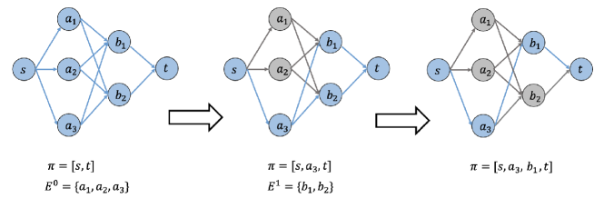
Figure 2: A visual illustration of Guided Pattern Refinement (GPR) in a toy example. We start with a pattern $\pi=[s,t]$ containing only the source and the target node. At each step we define a guided set $E^{0}$ and $E^{1}$, respectively and find the node in the guided set that maximize the pattern influence (Def. 3). GPR finally returns a pattern $\pi=[s,a_{3},b_{1},t]$ that abstracts a single path.

Definition 2 (Pattern)

A pattern $\pi$ is a sequence of nodes $[\pi_{1},\pi_{2},\cdots,\pi_{-1}]$ such that for any pair of nodes $\pi_{i},\pi_{i+1}$ adjacent in the sequence (not necessarily adjacent in the graph), there exists a path from $\pi_{i}$ and $\pi_{i+1}$.

A pattern $\pi$ abstracts a set of paths, written $\gamma(\pi)$ that follow the given sequence of nodes but are free to traverse the graph between those nodes in any way. Interpreting paths and patterns as sets, we define $\gamma(\pi)\stackrel{{\scriptstyle\smash{\scriptscriptstyle\mathrm{def}}}}{{=}}\left\{p\subseteq\mathcal{P}:\pi\subseteq p\right\}$ where $\mathcal{P}$ is the set of all paths from $\pi_{1}$ to $\pi_{-1}$. If every sequence-adjacent pair of nodes is directly connected then the pattern abstracts a single path. To quantify the amount of information that flows from the input node to the target node over a particular pattern, we propose Pattern Influence, motivated by distributional influence.

Definition 3 (Pattern influence)

Given a computation graph and a user-defined distribution $\mathcal{D}$, the influence of an influence pattern $\pi$, written $\mathcal{I}(\mathbf{x},\pi)$ is the total influence of all the paths abstracted by the pattern: $\mathcal{I}(\mathbf{x},\pi)\stackrel{{\scriptstyle\smash{\scriptscriptstyle\mathrm{def}}}}{{=}}\sum_{p\in\gamma(\pi)}\mathbb{E}_{\mathbf{z}\sim\mathcal{D}(\mathbf{x})}\prod^{-1}_{i=1}\frac{\partial p_{i}(\mathbf{z})}{\partial p_{i-1}(\mathbf{z})}$.

Proposition 1 (Chain Rule)

$\mathcal{I}(\mathbf{x},\pi)=\mathbb{E}_{\mathbf{z}\sim\mathcal{D}(\mathbf{x})}\prod_{i=1}^{-1}\frac{\partial\pi_{i}(\mathbf{z})}{\partial\pi_{i-1}(\mathbf{z})}$ for any distribution $\mathcal{D}(\mathbf{x})$.

Prop. 1 (proof in Appendix A) simplifies the evaluation of the pattern influence by specifying the exact set of internal nodes through which influence flows in a computational graph. We hereby introduce a greedy way of finding the most influential pattern in both $\mathcal{G}_{e}$ and $\mathcal{G}_{a}$.

Guided Pattern Refinement(GPR) Starting with source and target nodes $s$ and $t$ along with a initialized pattern $\pi^{0}=\left\{s,t\right\}$ representing all paths between $s$ and $t$, we construct $\pi^{1}$ by adding one sequence-adjacent node $e^{0}$ (there is a direct path between $s$ and $e^{0}$) from a guiding set $E^{0}$ that maximizes the influence of the resulting pattern such that:

$$e^{0}=\arg\max_{e\in E^{0}}\{\mathcal{I}(\mathbf{x},\left[s,e,t\right]),\pi^{1}=\left[s,e^{0},t\right],$$ (1)

This procedure is iterated until we exhaust the last guiding set. We show an example of GPR in a toy graph in Fig. 2. For an embedding-level graph $\mathcal{G}_{e}$, each guiding set $E^{l}$ includes all embeddings $\mathbf{h}^{l}_{1:N}$ at layer $l$. For the attention-level graph $\mathcal{G}_{a}$, we refine on the embedding-level pattern $\pi^{e}$ by only expanding $\pi^{e}$ from addition nodes in $\mathcal{G}_{a}$ compared with $\mathcal{G}_{e}$: we perform GPR iterations between $\pi^{e}_{l},\pi^{e}_{l+1}\in\pi^{e}$ with the guiding set $E^{l}_{a}$ which includes $A$ attention heads $\mathbf{a}^{l}$ and the skip node $\mathbf{s}^{l}$(Fig. 1 Right), until we reach the same last node in $\pi^{e}$. The returned attention-level pattern $\pi^{a}$ thus abstracts a single path from the source to the target in $\mathcal{G}_{a}$. As the attention-level analysis refines the embedding-level analysis, the produced attention-level pattern $\pi^{a}$ abstracts a strict subset of the paths of the attention-level graph that the embedding-level pattern $\pi^{e}$ abstracts. That is, $\pi^{e}\subset\pi^{a}$ while $\gamma(\pi^{a})\subset\gamma(\pi^{e})$. The detailed algorithm of GPR and analysis of its optimality can be found in Appendix B.1 and B.2.

4 Experiment

Experiments in this section demonstrate our method as a tool for interpreting end-to-end information flow in BERT. Specific visualizations exemplify these interpretations including the importance of skip connections and BERT’s encoding of grammatical concepts are included in Sec. 4.2. Sec. 4.3 explores the consistency of patterns across instances and template positions and how they relate to task performances and influence magnitudes in. Sec 4.4 demonstrates two advantages of patterns in explaining the information flow of BERT over baselines: 1) abstracted patterns, with much fewer nodes compared to the whole model, carry sufficient information for the prediction. That is, without the information outside the refined pattern, the model shows no significant performance drop; 2) At the same time, patterns are sparse but concentrated in BERT’s components.

4.1 Setup

Tasks. We consider two groups of NLP tasks: (1) subject-word agreement (SVA) and reflexive anaphora (RA). We explore different forms of sentence stimuli(subtask) within each task: object relative clause (Obj.), subject relative clause (Subj.), within sentence complement (WSC), and across prepositional phrase (APP) in SVA (marvin2018targeted, ); number agreement (NA) and gender agreement (GA) in RA (lin2019open, ). Both datasets are evaluated using masked language model (MLM) as is used in Goldberg goldberg2019assessing . We sample 1000 sentences from each subtask evenly distributed across different sentence types (e.g. singular/plural subject & singular/plural intervening noun) with a fixed sentence structure; (2) sentiment analysis(SA): we use 220 short examples (sentence length$\leq 17$) from the evaluation set of the 2-class GLUE SST-2 sentiment analysis dataset wang2018glue . More details and examples of each task can be found in Appendix D.1.

Models. For linguistic tasks, We evaluate our methods with a pretrained BERT($L=6,A=8$) turc2019 , referred hereby as $\text{BERT}_{\text{SMALL}}$. For SST-2 we fine-tuned on the pretrained $\text{BERT}_{\text{BASE}}$devlin2018bert with $L=12,A=12$. The models are similar in sizes compared to the transformer models used in abnar2020quantifying . All computations are done with a Titan V on a machine with 64 GB of RAM. See Appendix D.2 for more details.

Implementation of GPR. Let the target node for SVA and RA tasks be the output of the QoI score $q(\mathbf{y})\stackrel{{\scriptstyle\smash{\scriptscriptstyle\mathrm{def}}}}{{=}}y_{correct}-y_{wrong}$. For instance, $y_{\texttt{IS}}-y_{\texttt{ARE}}$ for the sentence she [MASK] happy. Similarly, we use $y_{\texttt{positive}}-y_{\texttt{negative}}$ for sentiment analysis. We choose an uniform distribution over a linear path from $\mathbf{x}_{b}$ to $\mathbf{x}$ as the distribution $\mathcal{D}$ in Def. 3 where the $\mathbf{x}_{b}$ is chosen as the the input embedding of [MASK] because it can viewed a word with no information. For a given input token $\mathbf{x}_{i}$, we apply GPR differently depending on the sign of distributional influence $g(\mathbf{x};q,\mathcal{D})$: if $g(\mathbf{x};q,\mathcal{D})\geq 0$, we maximize the pattern influence towards $q(\mathbf{y})$ at each iteration of the GPR otherwise we maximize pattern influence towards $-q(\mathbf{y})$. We use $\pi_{i}$ as the extracted patterns for individual input word $i$. When explaining the whole input sentence, we collect all refined patterns for each word and use $\Pi=\bigcup_{i}\pi_{i}$. Further, we denote $\Pi_{+}$ as the set of patterns for all positively influential words. Both terms may be further decorated by $a$ or $e$ to denote attention-level or embedding-level results.

4.2 Visualizing Influence Patterns

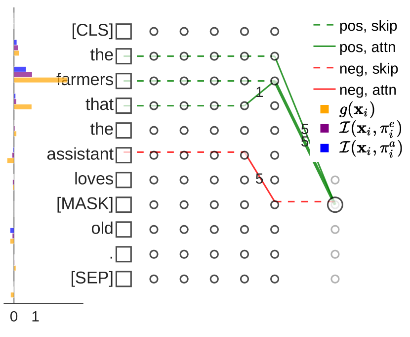
(a) plural subject+singular attractor(PS)

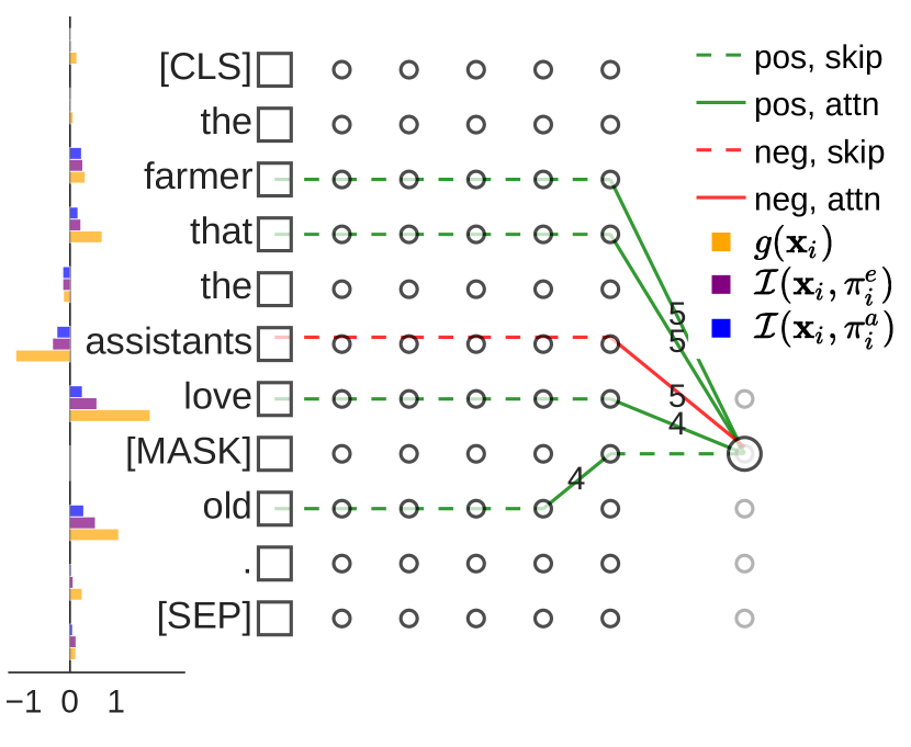
(b) singular subject+plural attractor(SP)

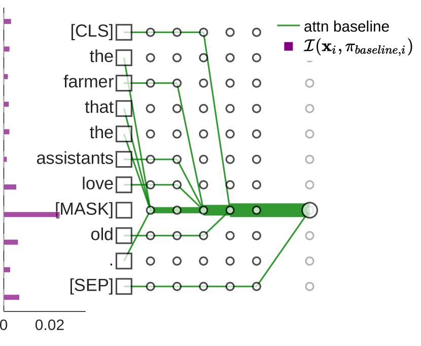
(c) attention-based baseline $\Pi_{\text{attn}}$

Figure 3: (a)(b) Patterns for two instances of SVA-Obj.(c)Baseline pattern $\Pi_{\text{attn}}$. For each plot: Left: bar plots of the distributional influence $g(\mathbf{x}_{i})$(yellow), $\mathcal{I}(\mathbf{x}_{i},\pi^{e}_{i})$ (purple) and $\mathcal{I}(\mathbf{x}_{i},\pi^{a}_{i})$ (blue) (or $\mathcal{I}(\mathbf{x}_{i},\pi_{baseline,i})$) for each word at position $i$. Right: Extracted patterns $\Pi$ from selective words. Square nodes and circle nodes denote input and internal embeddings, respectively. In (a) and (b), influence flowing through skip connections is represented by dashed lines and attention heads in solid lines; the edges are are marked with the corresponding attention head number (ranging from 1 to $A$) in $\Pi^{a}$ . Line colors represent the sign of influence (red as negative and green as positive).

This section does not serve as an evaluation but an exploration of insightful results and succinct conclusions an human user can learn from our proposed technique. We visualize the information flow identified by patterns found by GPR, and compare with those generated by attention weights as explored in the literature abnar2020quantifying ; wu2020structured . We therefore use $\Pi_{\text{attn}}$ to denote a pattern of nodes by maximizing the product of the corresponding attention weights between each pairs of nodes from adjacent layers. Implementation details are included in Appendix C.1.

We first focus on instances of the subtask SVA across object relative clauses (SVA-obj), which are generated from the template: the SUBJECT that the ATTRACTOR VERB [MASK](is/are) ADJ.. We observe in Figure 3 that the subject words exert positive input influences on the correct choice of the verb, and the intervening noun (attractor) exerts negative influence, which is true for both $\mathcal{I}(\mathbf{x}_{i},\pi^{e}_{i})$ and $\mathcal{I}(\mathbf{x}_{i},\pi^{a}_{i})$ (blue and purple bars in Figure 3(a) and 3(b)). While $\Pi_{\text{attn}}$(Fig. 3(c)) does not distinguish between positively influential words and negative ones, nor do they show an interpretable pattern. Our other main findings are discussed as follows.

Finding I: Skip Connection Matters.

Horizontal dashed lines in Figure 3 indicate that influence can flow through layers at the same word position via skip connections, which is not isolated as separate nodes $\Pi_{\text{attn}}$ (shown in Fig. 3(c)). Fig. 3(a) and 3(b) also show that the influence from subject words farmer[s] travels through skip connections across layers before it transfers into the attention head 5 in the last layer, indicating the “number information” from the subject embedding flows directly to the output. Interestingly, this also explains why attentions can be pruned effectively without compromising the performance kovaleva2019revealing ; michel2019sixteen ; voita2019analyzing as important information may not flow through attentions at all. Namely, they are simply “copied” to the next layer through the skip connection. In fact, attention heads are traversed far less often than skip connections, which account for $75.4\%$ of nodes in $\Pi_{a}$ across all tasks evaluated.

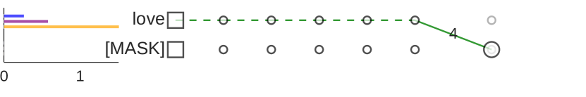
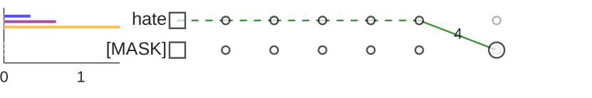
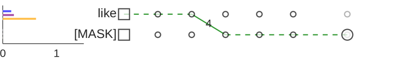
(a) Interactions between clausal verbs & [MASK] for SVA-Obj

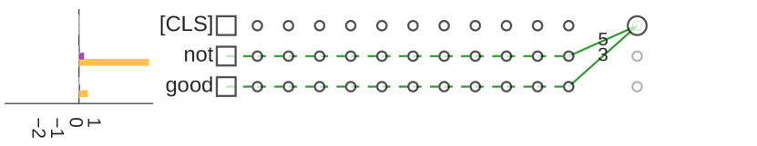
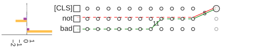
(b) Interactions between not & adjectives in SA

Figure 4: (a) Patterns on three clausal verbs from SP, SVA-obj.(b) Patterns for two instances in the SA task. Legend follows Figure 3.

Finding II: that as an Attractor.

Fig. 3(a) and 3(b) shows that the singular subject is less influential than the plural subject, especially when compared to the large negative influence from the attractor. Besides, the word that behaves like a singular pronoun in the singular subject case (Figure 3(b)), flowing through the same pattern as the subject (skip connections + attention head 5), whereas that is more like a grammatical marker (relativizer) in the plural subject case (Figure 3(a)): the pattern from that converge to the subject in the second to last layer via a different attention head 1. An explanation to the observed difference is that that can either be used as a singular pronoun in English, or a marker that encodes the syntactic boundary of the clause to help identify the subject and ignore the attractor. This finding reveals that although the latter one is always the correct usage for that across all instances, BERT may resort to the “easier”(while ungrammatical) encoding of that as a pronoun when the number happens to be singular.

Finding III: love, hate and like

Figure 4(a) shows the pattern across three instances containing different clausal verbs by replacing love in Figure 3(b) with like or hate. We observe that hate and love are more influential, with a distinct and more concentrated pattern compared to that of the word like, while one comparable to that of the subject or noun attractor. Therefore, hate and love are treated more like singular nouns than like, contributing positively to the correct prediction of the verb’s number (but for the wrong grammatical reason). This discrepancy also corroborates different accuracy for instances in the three subsets: hate: .99; love: 1.0; like: .82. In fact, the number of misclassifications containing like accounts for more than $33\%$ of all misclassifications in SVA-Obj(SP).

Finding IV: Interactions with not. Two instances of sentiment analysis which BERT classifies correctly (negative for not good. and positive for not bad.) in Fig. 4(b) shows that: 1) in not good., not and good does not interact internally and not carries much more positive influence than good towards the correct class (negative sentiment); 2) in not bad., on the contrary, not contributes negatively to the correctly class (positive sentiment) and bad interacts with the not in an internal layer and exhibit a large positive influence. This disparity shows the model may treat not as a word with negative sentiment by default, and only when the subsequent adjective is negative, can it be used as a negation marker to encode the correct sentiment.

The asymmetries and oddities of patterns of Finding II to IV show how BERT may use ungrammatical correlations for its predictions. We include more examples of patterns in Appendix E.

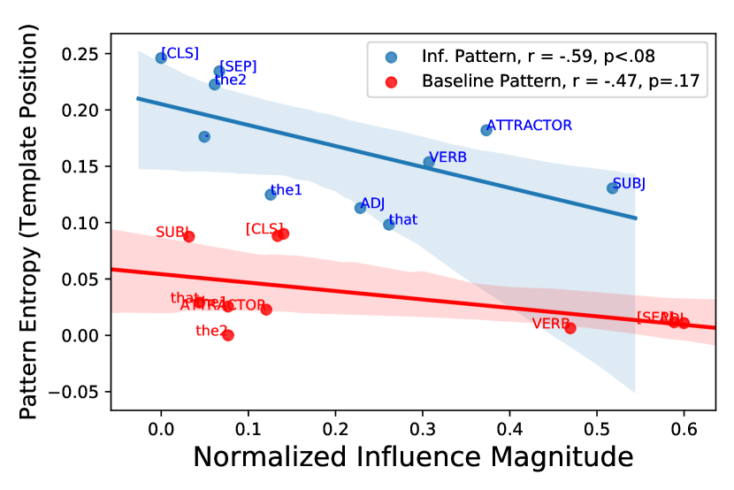
(a) Pattern Entropy vs. Average Influence Magnitude for template positions in SVA-Obj

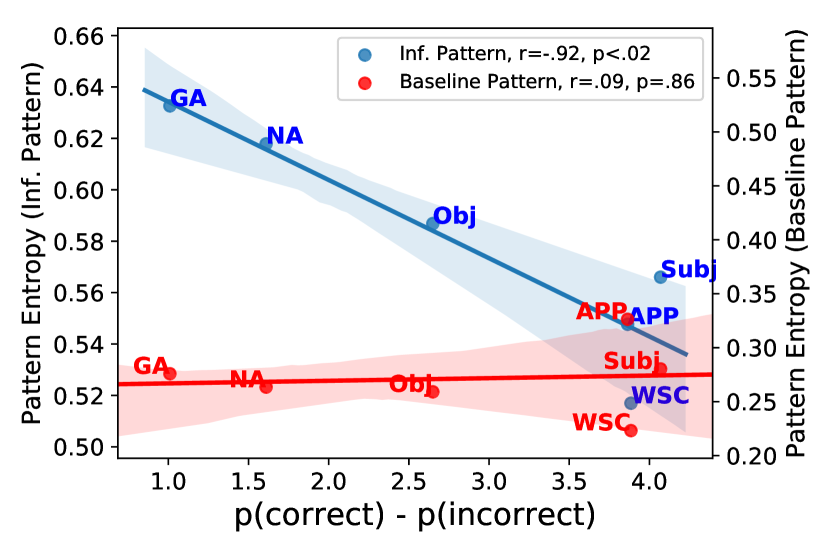
(b) Pattern Entropy vs. Average QoI for linguistic tasks (SVA & RA)

Figure 5: Relationship between Task Performance, Influence Magnitude and Pattern Entropy

4.3 Consistency of Patterns Across Instances

The prior section offered examples building connections between information flow and patterns. Since patterns are computed for each word of each instance individually, a global analysis of consistency/variation of patterns across instances can help us make deeper insights and make more general conjectures. We quantify this variation with pattern entropy on the linguistic tasks (SVA & RA) with fixed templates, where for each instance, each template position are chosen from a group of words. Interpreting the collection of instances, or template positions, in a task as a distribution, pattern entropy is the entropy of the binary probability that a node is part of a pattern, averaged over all nodes (minimally this is 0 if all patterns incorporate the exact same set of nodes). With a node $n$ in graph $G$, a set of $K$ instances, $\pi_{k}$ as the pattern of instance $k$ by abuse of notation and $H$ as the entropy function: pattern entropy of a pattern $\pi$ is defined as:

$$\hat{H}(\pi,G)=\frac{\sum_{n\in G}H(p_{n}(\pi))}{|G|};p_{n}(\pi)=\frac{\sum_{k}\mathbbm{1}(n\in\pi_{k})}{K}$$

Figure 5(a) shows an inverse linear relation between influence magnitude and the pattern entropy of each template position($\pi_{i}$) in SVA-Obj. For example, the subject position has on average high influence magnitude and low pattern entropy, while grammatically unimportant template positions such as [CLS] and the period token has relatively low influence and high entropy. Note that this fit is not perfect: attractors, for example, have high influence magnitude but also high entropy’s due to their disparate behaviors among instances shown in Sec 4.2.

Figure 5(b) demonstrates a more global inverse relation between the pattern entropy of $\Pi_{+}$ and task-specific performance(average QoI) for 6 linguistic subtasks studied. This indicates that the more consistent a pattern is for a concept, i.e, the more consistent how a model locates the positively influential signals, the better the model is at capturing that concept. In both figures, the baseline attention-based patterns ($\Pi_{\text{attn}}$) does not indicate this relation. Together with Finding II to IV in Sec. 4.2, it demonstrates that patterns may offer alternative insights in formalizing and answering high-level questions such as to what extent does BERT generalize to correct and consistent grammatical rules or use spurious correlations which varies across instancesmccoy2019right ; mccoy2020berts ; ribeiro2020beyond .

4.4 Evaluating Influence Patterns

This section serves as a formal evaluation of our proposed methods against existing baselines in tracing information flows. Except the attention baseline $\Pi_{\text{attn}}$ defined in Sec. 4.2, we also include the following baselines (implementation details to follow in Appendix C.1):

$\blacksquare$ $\Pi_{\text{rand}}$: patterns with randomly sampled nodes.

$\blacksquare$ $\Pi_{\text{inf}}$: patterns consisting of nodes that maximize the internal influence leino2018influence for each guiding set.

$\blacksquare$ $\Pi_{\text{cond}}$: patterns consisting of nodes that maximize the conductance dhamdhere2018important for each guiding set.

We compare various aspects of extracted patterns against the following baselines, including: (1) ablation experiments showing how influence patterns account for model performance; (2) the sparsity of the patterns in the computational graph. Finally, we also discuss the relation between patterns and attention-weights.

Patterns	SVA				RA		SA
	Obj.	Subj.	WSC	APP	NA	GA
$\Pi^{e}_{+}$(ours)	.96	.99	1.0	.96	.98	.99	.97
$\Pi^{e}_{\text{rand}}$	.55	.60	.55	.55	.55	.56	.52
$\Pi^{e}_{\text{attn}}$	.61	.55	.49	.63	.56	.65	.47
$\Pi^{e}_{\text{cond}}$	.93	.91	.88	.90	.71	.95	.94
$\Pi^{e}_{\text{inf}}$	.66	.71	.50	.56	.68	.50	.49
$\Pi^{a}_{+}$(ours)	.70	.62	.56	.65	.78	.89	.86
$\Pi^{a}_{\text{rand}}$	.50	.50	.50	.50	.50	.50	.49
$\Pi^{a}_{\text{repl\_skip}}$	.50	.58	.54	.52	.55	.50	.48
original	.96	1.0	1.0	1.0	.83	.73	.92

Metrics	SVA				RA		SA
	Obj.	Subj.	WSC	APP	NA	GA
conc.(${\Pi_{+}^{e}}$)	.33	.30	.27	.33	.31	.22	.07
conc.(${\Pi_{-}^{e}}$)	.29	.30	.38	.31	.31	.23	.05
share(${\Pi_{+}^{e}}$)	.06	.09	.03	.06	.04	.02	.01
conc.(${\Pi_{+}^{a}}$)	.21	.18	.16	.18	.18	.14	.01
conc.(${\Pi_{-}^{a}}$)	.17	.16	.25	.15	.17	.15	.01
share(${\Pi_{+}^{a}}$)	1.8	1.7	1.6	1.5	1.3	1.3	3e-2
$(\cdot 10^{-6})$
Alignment	.58	.57	.57	.59	.46	.53	.34
Rate

Table 1: Summary of quantitative results, with $*\in\{e,a\}$, denoting embedding & attention-level metrics. Left: Ablated accuracies of $\Pi_{+}$ and baseline patterns. Right: Sparsity metrics; conc.(${\Pi_{\pm}^{*}}$): positive/negative concentration; share(${\Pi^{*}}$): path share of pattern ${\Pi^{*}}$.

Ablation. We extend the commonly-used ablation study for evaluating explanation methods (deyoung2020eraser, ; Dabkowski2017RealTI, ; ancona2018towards, ; leino2018influence, ; DBLP:conf/acl/LuMLFD20, ) from input features to internal patterns as a sanity check of our method. That is, we ablate BERT down to a simpler model: we only retain the nodes from $\Pi_{+}^{e}$ (or $\Pi_{+}^{a}$) while replacing other nodes by zeros. The retained and replaced nodes together are forward passed to the next layer with the original model parameters until a new set of nodes are retained or replaced. Ablated Accuracy denotes the accuracy of the ablated model. We show the results for our methods $\Pi^{*}_{+}$ and other baseline patterns in Table 1. Each baseline retains the same number of nodes as the corresponding $\Pi_{+}$. Although this process seems to be highly invasive, the model ablated with $\Pi^{*}_{+}$ achieved the highest ablated accuracy uniformly over all tasks. All baseline patterns except $\Pi_{\text{cond}}^{e}$ gives random guesses. For the attention-level graph $\Pi_{a}$, we also add a counterfactual pattern $\Pi^{a}_{\text{repl\_skip}}$ where we replace each skip node in $\Pi^{a}_{+}$ with its all $A$ corresponding attention heads. However, with much fewer nodes ablated, $\Pi^{a}_{\text{repl\_skip}}$ still produces random ablated accuracies. This corroborates Finding I in Sec. 4.2 that the skip connections relaying important information directly which attention block cannot replace. In summary, patterns refined by GPR account for the model’s information flow more sufficiently compared to all baselines.

Sparsity of Patterns. A good explanation should not only account for the model performance, but also be sparse relative to the entire model semantics so as to be interpretable to humans. In this section, we quantify the sparsity of extracted patterns using two metrics: path share and concentration. With on average more than 10 words per sentence, the embedding and attention-level graphs contain at least $10^{6}$ and $10^{11}$ individual paths, respectively. The totality of these paths represent the entire semantics of the BERT model. Path share(i.e. $\text{share}(\Pi_{+}^{*})\stackrel{{\scriptstyle\smash{\scriptscriptstyle\mathrm{def}}}}{{=}}|\gamma_{*}(\Pi^{*}_{+})|/|\mathcal{P}^{*}|$), is defined as the number of paths in a pattern over the total number of paths in the entire computational graph. concentration, on the other hand, is defined as the proportion of negative/positive pattern influence over the total positive/negative influence. It represents the average ratio between the blue/purple bars and the orange bars in Figure 3.

Table 1(Right) shows that the abstracted patterns contain only a small share of paths while accounting for a large portion of both positive and negative influence. In linguistic tasks, the embedding level abstracted pattern has a concentration around $0.3$ (conc.(${\Pi_{\pm}^{e}}$)), indicating that the input concept flows through single internal embeddings in each layer, instead of distributed to many words. Zooming in on the attention-level graph, a relative high concentration conc.(${\Pi_{+}^{a}}$), suggests that between the internal embeddings of adjacent layers, influence is also more concentrated to either one attention head or the skip connection. We speculate the much lower conc.(${\Pi_{+}}$) in SA is due to (1) the much larger model for the SA task with more layers and attention heads (2) sentiment information may be more diverse and complex than the information needed to encode syntax agreements, therefore input information may flow in a more distributed way. However, despite low concentration of pattern influence, the extracted patterns for SA are still effective in capturing the model performance as shown in Table 1(Left).

Attention heads in $\Pi^{a}$ vs. Attention weight value. Another observation is that the attention head nodes in $\Pi^{a}$ found by GPR aligns, to greater extent than random ($1/|A|$), with the head of the largest attention weight along the corresponding embedding-level edge, as shown by alignment rate in Table 1(Left). This partial alignment is expected since the Jacobian between two nodes correlates with the coefficients (weights) in the linear attention mechanism(product rule), while the opposite is also expected since (1) attention weights themselves are not fixed model parameters thus part of the gradient flow, (2) model components other than attention blocks come between two adjacent layers (e,g. dense layer & skip connections). In other words, attention weights are correlated, but not equivalent to gradient-based methods as explanations.

5 Related Work

Previous work has shown the encoding of syntactic dependencies such as SVA in RNN Language models (linzen2016assessing, ; hupkes2018visualisation, ; lakretz2019emergence, ; jumelet2019analysing, ). More extensive work has since been done on transformer-based architectures such as BERT. Probing classifiers has shown BERT encodes many types of linguistic knowledge(elazar2020bert, ; hewitt2019designing, ; tenney2019bert, ; tenney2019you, ; jawahar2019does, ; klafka2020spying, ; liu2019linguistic, ; lin2019open, ; coenen2019visualizing, ; hewitt2019structural, ). goldberg2019assessing discovers that SVA and RA in complex clausal structures is better represented in BERT compared to an RNN model.

A line of related works analyze self-attention weights of BERT(clark2019does, ; vig2019analyzing, ; lin2019open, ; ethayarajh2021attention, ), where attention heads are found to have direct correspondences with specific dependency relations. abnar2020quantifying and wu2020structured , with which we compare in this paper, propose using attentions to quantify information flows in BERT. Attention weights as interpretation devices, however, have been controversial (serrano2019attention, ) and empirical analysis has shown that attention can be perturbed or pruned while retaining performance (kovaleva2019revealing, ; michel2019sixteen, ; voita2019analyzing, ). Our work demonstrates that attention mechanisms are only part of the computation graph, with each attention block complemented by other model components such as dense layer and skip connections; axiomatically justified influence patterns, however, can attribute to the whole computation graph. The strong influence passing through skip connections also corroborates the findings of brunner2020identifiability which finds input tokens mostly retain their identity. Besides pruning attentions, other worksprasanna2020bert ; sanh2019distilbert ; jiao2019tinybert also show that BERT is overparametrized and can be greatly compressed. Our work to some extent corroborates that point by pointing to the sparse gradient flow, while employing ablation studies only to verify the sufficiency of the extracted patterns.

A closely related and concurrent workpmlr-v139-dong21a also shows the importance of skip connections and dense(MLP) layers by decomposing and analyzing forward-pass computations in self-attention modules. Our work, in comparison, introduces a gradient-based method that can be generalized to any model as long as they are differentiable. We also focus on how influential patterns can help us understand information flow of specific NLP tasks.

Recent work introducing influence paths (DBLP:conf/acl/LuMLFD20, ) offers another form of explanation. Lu et al. DBLP:conf/acl/LuMLFD20 decomposed the attribution to path-specific quantities localizing the implementation of the given concept to paths through a model. The authors demonstrated that for LSTM models, a single path is responsible for most of the input-output effect defining SVA. Directly applying individual paths to transformer-based models like BERT, however, results in an intractable number of paths to enumerate due to the huge number of computation edges in BERT.

6 Limitations and Future Work

We believe there are three limitations to address in future work. (1) GPR algorithm does not guarantee absolute optimality, however, we provide empirical evidence in support of the searching algorithm in Appendix B.2. (2) For interpretability reasons, we compute GPR by picking one node per guiding set, while more complicated information may distribute to multiple internal embeddings or attention heads. (3) The findings in Sec. 4.2 would benefit from more quantitative analysis to support more general claims(instead of speculations) on BERT’s handling of various linguistic/semantic concepts. However, we will explore these limitations in future work and release our code and hope the proposed methods will serve as an insightful tool in future exploration.

7 Conclusion

We demonstrated influence patterns for explaining information flow in BERT. We highlighted the importance of skip connections and BERT’s potentially mishandling of various concepts through visualized patterns. We inspected the relation between consistency of patterns across instances with model performance and quantitatively validated pattern’s sufficiency in capturing model performance.

Acknowledgement

This work was developed with the support of NSF grant CNS-1704845. The U.S. Government is authorized to reproduce and distribute reprints for Governmental purposes not withstanding any copyright notation thereon. The views, opinions, and/or findings expressed are those of the author(s) and should not be interpreted as representing the National Science Foundation or the U.S. Government. We gratefully acknowledge the support of NVIDIA Corporation with the donation of the Titan V GPU used for this work.

Checklist

1. For all authors…

   1. Do the main claims made in the abstract and introduction accurately reflect the paper’s contributions and scope? [Yes]

   2. Did you describe the limitations of your work? [Yes] , in Sec. 6

   3. Did you discuss any potential negative societal impacts of your work? [Yes] , in Appendix E.3

   4. Have you read the ethics review guidelines and ensured that your paper conforms to them? [Yes]

2. If you are including theoretical results…

   1. Did you state the full set of assumptions of all theoretical results? [Yes] Only one theoretical result (Prep. 1 in in Sec. 3)

   2. Did you include complete proofs of all theoretical results? [Yes] A simple proof is included in Appendix A

3. If you ran experiments…

   1. Did you include the code, data, and instructions needed to reproduce the main experimental results (either in the supplemental material or as a URL)? [Yes] In Sec. 4. More details in the appendix D.

   2. Did you specify all the training details (e.g., data splits, hyperparameters, how they were chosen)? [Yes] In Sec. 4. More details in the appendix  D.

   3. Did you report error bars (e.g., with respect to the random seed after running experiments multiple times)? [Yes] . The only random experiments are done for Table 1, the error statistics are included in C.3.

   4. Did you include the total amount of compute and the type of resources used (e.g., type of GPUs, internal cluster, or cloud provider)? [Yes] In Sec. 4. More details in the appendix D.

4. If you are using existing assets (e.g., code, data, models) or curating/releasing new assets…

   1. If your work uses existing assets, did you cite the creators? [Yes] In In Sec. 4.

   2. Did you mention the license of the assets? [Yes] . in the appendix D.

   3. Did you include any new assets either in the supplemental material or as a URL? [Yes] . Code included in the supplementary materials.

   4. Did you discuss whether and how consent was obtained from people whose data you’re using/curating? [N/A] .

   5. Did you discuss whether the data you are using/curating contains personally identifiable information or offensive content? [N/A]

5. If you used crowdsourcing or conducted research with human subjects…

   1. Did you include the full text of instructions given to participants and screenshots, if applicable? [N/A]

   2. Did you describe any potential participant risks, with links to Institutional Review Board (IRB) approvals, if applicable? [N/A]

   3. Did you include the estimated hourly wage paid to participants and the total amount spent on participant compensation? [N/A]

Appendix A Appendix: Proof of Proposition 1

Proposition 1 (Chain Rule) $\mathcal{I}(\mathbf{x},\pi)=\mathbb{E}_{\mathbf{z}\sim\mathcal{D}(\mathbf{x})}\prod_{i=1}^{-1}\frac{\partial\pi_{i}(\mathbf{z})}{\partial\pi_{i-1}(\mathbf{z})}$ for any distribution $\mathcal{D}(\mathbf{x})$.

We first show that for a pattern $\pi=[\pi_{1},\pi_{1},...,\pi_{k},...,\pi_{n}]$ the following equation holds:

$$\frac{\partial\pi_{n}}{\partial\pi_{1}}=\frac{\partial\pi_{n}}{\partial\pi_{k}}\frac{\partial\pi_{k}}{\partial\pi_{1}}$$ (2)

Proof: Let $\gamma(\pi_{1}\rightarrow\pi_{n})$ be a set of paths that the pattern $\pi$ abstracts. Therefore, we have

$$\frac{\partial\pi_{n}}{\partial\pi_{1}}=\sum_{p\in\gamma(\pi_{1}\rightarrow\pi_{n})}\prod^{-1}_{i=1}\frac{\partial p_{i}}{\partial p_{i-1}}$$ (3)

Similarly, we have

$$\frac{\partial\pi_{k}}{\partial\pi_{1}}=\sum_{p\in\gamma(\pi_{1}\rightarrow\pi_{k})}\prod^{-1}_{i=1}\frac{\partial p_{i}}{\partial p_{i-1}},\quad\frac{\partial\pi_{n}}{\partial\pi_{k}}=\sum_{p\in\gamma(\pi_{k}\rightarrow\pi_{n})}\prod^{-1}_{i=1}\frac{\partial p_{i}}{\partial p_{i-1}}$$ (4)

Suppose $|\gamma(\pi_{1}\rightarrow\pi_{k})|=N_{1}$, $|\gamma(\pi_{k}\rightarrow\pi_{n})|=N_{2}$ and we denote $\prod^{-1}_{i=1}\frac{\partial p^{(j)}_{i}}{\partial p_{i-1}}$ as path gradient flowing from the path $j$. Therefore,

$$\frac{\partial\pi_{n}}{\partial\pi_{1}} =\sum_{p\in\gamma(\pi_{1}\rightarrow\pi_{n})}\prod^{-1}_{i=1}\frac{\partial p_{i}}{\partial p_{i-1}}$$ (5)

$$=\prod^{-1}_{i=k}\frac{\partial p^{(1)}_{i}}{\partial p_{i-1}}\cdot\prod^{k}_{i=1}\frac{\partial p^{(1)}_{i}}{\partial p_{i-1}}+\prod^{-1}_{i=k}\frac{\partial p^{(1)}_{i}}{\partial p_{i-1}}\cdot\prod^{k}_{i=1}\frac{\partial p^{(2)}_{i}}{\partial p_{i-1}}+...+\prod^{-1}_{i=k}\frac{\partial p^{(1)}_{i}}{\partial p_{i-1}}\cdot\prod^{k}_{i=1}\frac{\partial p^{(N_{1})}_{i}}{\partial p_{i-1}}$$ (6)

$$+\prod^{-1}_{i=k}\frac{\partial p^{(2)}_{i}}{\partial p_{i-1}}\cdot\prod^{k}_{i=1}\frac{\partial p^{(1)}_{i}}{\partial p_{i-1}}+\prod^{-1}_{i=k}\frac{\partial p^{(2)}_{i}}{\partial p_{i-1}}\cdot\prod^{k}_{i=1}\frac{\partial p^{(2)}_{i}}{\partial p_{i-1}}+...+\prod^{-1}_{i=k}\frac{\partial p^{(2)}_{i}}{\partial p_{i-1}}\cdot\prod^{k}_{i=1}\frac{\partial p^{(N_{1})}_{i}}{\partial p_{i-1}}$$ (7)

$$+...$$ (8)

$$+\prod^{-1}_{i=k}\frac{\partial p^{(N_{2})}_{i}}{\partial p_{i-1}}\cdot\prod^{k}_{i=1}\frac{\partial p^{(1)}_{i}}{\partial p_{i-1}}+\prod^{-1}_{i=k}\frac{\partial p^{(N_{2})}_{i}}{\partial p_{i-1}}\cdot\prod^{k}_{i=1}\frac{\partial p^{(2)}_{i}}{\partial p_{i-1}}+...+\prod^{-1}_{i=k}\frac{\partial p^{(N_{2})}_{i}}{\partial p_{i-1}}\cdot\prod^{k}_{i=1}\frac{\partial p^{(N_{1})}_{i}}{\partial p_{i-1}}$$ (9)

$$=\sum^{N_{2}}_{j}(\prod^{-1}_{i=k}\frac{\partial p^{(j)}_{i}}{\partial p_{i-1}}\cdot\sum^{N_{1}}_{m}\prod^{k}_{i=1}\frac{\partial p^{(m)}_{i}}{\partial p_{i-1}})$$ (10)

$$=\sum^{N_{2}}_{j}(\prod^{-1}_{i=k}\frac{\partial p^{(j)}_{i}}{\partial p_{i-1}})\cdot\sum^{N_{1}}_{m}(\prod^{k}_{i=1}\frac{\partial p^{(m)}_{i}}{\partial p_{i-1}})$$ (11)

$$=\sum_{p\in\gamma(\pi_{1}\rightarrow\pi_{k})}\prod^{-1}_{i=1}\frac{\partial p_{i}}{\partial p_{i-1}}\cdot\sum_{p\in\gamma(\pi_{k}\rightarrow\pi_{n})}\prod^{-1}_{i=1}\frac{\partial p_{i}}{\partial p_{i-1}}$$ (12)

$$=\frac{\partial\pi_{n}}{\partial\pi_{k}}\frac{\partial\pi_{k}}{\partial\pi_{1}}$$ (13)

Now we prove Proposition 1.

$$\mathcal{I}(\mathbf{x},\pi) =\sum_{p\in\gamma(\pi)}\mathbb{E}_{\mathbf{z}\sim\mathcal{D}(\mathbf{x})}\prod^{-1}_{i=1}\frac{\partial p_{i}(\mathbf{z})}{\partial p_{i-1}(\mathbf{z})}$$ (14)

$$=\mathbb{E}_{\mathbf{z}\sim\mathcal{D}(\mathbf{x})}\sum_{p\in\gamma(\pi)}\prod^{-1}_{i=1}\frac{\partial p_{i}(\mathbf{z})}{\partial p_{i-1}(\mathbf{z})}$$ (15)

$$=\mathbb{E}_{\mathbf{z}\sim\mathcal{D}(\mathbf{x})}\prod_{i=1}^{-1}\frac{\partial\pi_{i}(\mathbf{z})}{\partial\pi_{i-1}(\mathbf{z})}$$ (16)

Appendix B Appendix: Guided Pattern Refinement

B.1 Algorithms for GPR

The pseudo code of the GPR algorithms are presented in algorithm 1 and 2.

Result: Significant Path $\pi^{e}$

initialization;

$\mathbf{x}\sim\text{Input Tokens}$, $f\leftarrow\text{BERT}$ ;

$\mathcal{G}_{e}\leftarrow\text{GetEmbeddingGraph}(f)$, $L\leftarrow\text{GetNumberOfLayers}(f)$;

$N\leftarrow\text{GetNumberOfTokens(f)}$, $m\leftarrow\text{GetIndex}(\texttt{[MASK]})$, ;

$n_{q}\leftarrow\text{GetQoINode($m,\mathcal{G}_{e}$)}$, $n_{w}\leftarrow\text{GetClfNode($\mathcal{G}_{e}$)}$;

$\pi^{e}\leftarrow\text{OrderedSet()}$, $\mathcal{C}\leftarrow\{\}$ ;

$j\leftarrow\text{GetStartingIndex()}$;

  // The word we start the search with

$n^{0}_{j}\leftarrow\text{GetNode}(\mathcal{G}_{w},\mathbf{h}^{0}_{j})$ ;

  // Find the corresponding node

$\pi^{e}\leftarrow\text{Append}(\pi^{e},n^{0}_{j})$;

for $l\in\{1,...,L-2\}$ do

       $\mathcal{C}\leftarrow\{\}$;

       for $i\in\{0,...,N-1\}$ do

             $n^{l}_{i}\leftarrow\text{GetNode}(\mathcal{G}_{w},\mathbf{h}^{l}_{i})$ ;

             $\pi_{t}\leftarrow\text{Append}(\pi,n^{l}_{i})$;

             $\mathcal{C}\leftarrow\mathcal{C}\cup\{\pi_{t}\}$ ;

            

       end for

      $\pi^{e}\leftarrow\arg\max_{\pi^{\prime}\in\mathcal{C}}\mathcal{I}(\mathbf{x}|\pi^{\prime},\pi^{\prime}_{-1}\rightarrow^{\mathcal{P}}n_{q})$

end for

$n^{L}_{m}\leftarrow\text{GetNode}(\mathcal{G}_{w},\mathbf{h}^{L-1}_{m})$;

$\pi^{e}\leftarrow\text{Append}(\pi^{e},n^{L}_{m})$;

$\pi^{e}\leftarrow\text{Append}(\pi^{e},n_{w})$;

$\pi^{e}\leftarrow\text{Append}(\pi^{e},n_{q})$;

Algorithm 1 Guided Pattern Refinement in the Embedding-level Graph (GPR-e)

Result: Significant Path $\pi^{a}$

initialization;

$\mathbf{x}\sim\text{Input Tokens}$, $f\leftarrow\text{BERT}$ ;

$\mathcal{G}_{e}\leftarrow\text{GetEmbeddingGraph}(f)$, $\mathcal{G}_{a}\leftarrow\text{GetAttentionGraph}(f)$;

$m\leftarrow\text{GetIndex}(\texttt{[MASK]})$;

$n_{q}\leftarrow\text{GetQoINode($m,\mathcal{G}_{e}$)}$;

$L\leftarrow\text{GetNumberOfLayers}(f)$, $N\leftarrow\text{GetNumberOfTokens(f)}$ ;

$\pi^{e}\leftarrow\text{GPR-e}(\mathbf{x},\mathcal{G}_{e})$;

  // Find embedding-level path first

$\mathcal{C}\leftarrow\{\}$;

for $i\in\{0,...,|\pi^{e}|-2\}$ do

       if ExistAttentionBlock($\pi^{e}_{i},\pi^{e}_{i+1}$);

        // Check if this is a Transformer Layer

       then

             $\mathcal{A}_{i}\leftarrow\text{GetHeadsBetween}(\mathcal{G}_{a},\pi^{e}_{i},\pi^{e}_{i+1})$;

              // Get all attention heads and the skip connetion node

             $\pi^{e}_{head}\leftarrow\text{Slice}(\pi^{e}_{0},\pi^{e}_{i})$;

              // Take a slice between two nodes

             $(a^{*}_{i},c^{*}_{i})\leftarrow\arg\max_{(a_{i},c_{i})\in\mathcal{A}_{i}}\mathcal{I}(\mathbf{x}|\pi^{e}_{head}\cup\{a_{i},c_{i}\},c_{i}\rightarrow^{\mathcal{P}}n_{q})$;

             $\mathcal{C}\leftarrow\mathcal{C}\cup\{(a^{*}_{i},c^{*}_{i})\}$;

            

      else

             continue;

            

       end if

      

end for

$\pi^{a}\leftarrow\text{InsertNode}(\pi^{e},\mathcal{C})$;

  // Insert attention nodes into the embedding-level path at the corresponding place

Algorithm 2 Guided Pattern Refinement in the Attention-level Graph (GPR-a)

B.2 Optimality of GPR

The definition of pattern influence does not allow for polynomial-time searching algorithms such as dynamic programming. (Such an algorithm is possible for simple gradients/saliency maps but not for integrated gradients due to the expectation sum over the multiplication of Jacobians along all edges). As for the optimality of the polynomial-time greedy algorithm, we hereby include a statistical analysis by randomly sampling 1000 alternative patterns for 100 word patterns in the SVA-obj task and sentiment analysis task (SST2). The pattern influence of those random paths shows that the patterns extracted GPR are (1) more influential than 999.96 and 1000(all) random patterns, averaged across all 100 word patterns evaluated for embedding-level attention-level patterns, respectively for SVA-obj; the same holds for sentiment analysis (1000 and 1000); (2) The extracted pattern influences are statistically significant assuming all randomly sampled patterns’ influences follow a normal distribution, with $p=$2e-10 for and $p=0$ for embedding-level and attention-level patterns, respectively for SVA-obj; the same holds for sentiment analysis ($p=0$ for and $p=0$). In other words, the pattern influence values are far more significant than a random pattern, also confirmed by the high concentration values shown in  Sec. 4.4.

Appendix C Appendix: Baseline Patterns

C.1 Baseline: Attention-based baseline

We introduce the implementation details of attention-based patterns, inspired by [2] and [49]. Consider a BERT model with $L$ layers, between adjacent layers $l$ and $l+1$, the attention matrix is denoted by $M_{l}\in\mathbb{R}^{A\times N\times N}$ where $A$ is the number of attention heads and $K$ is the number of embeddings. Each element of $M_{l}[a,i,j]$ is the attentions scores between the $i$-th embedding at layer $l$ and the $j$-th embedding at layer $l+1$ of the $a$-th head such that $\sum_{i}M_{l}[a,i,j]=1$. We average the attentions scores over all heads to lower the dimension of $M$: $\tilde{M}_{l}\stackrel{{\scriptstyle\smash{\scriptscriptstyle\mathrm{def}}}}{{=}}\frac{1}{A}\sum_{a}M_{l}[a]$. We define the baseline attention path as a path where the product of each edge in this path is the maximum possible score among all paths from a given source to the target.

Definition 4 (Attention-based Pattern)

Given a set of attention matrices $\tilde{M}_{0},\tilde{M}_{1},...,\tilde{M}_{L-1}$, a source embedding $x$ and the quantity of interest node $q$, an attention-based pattern $\Pi_{\text{attn}}$ is defined as

$$\Pi_{\text{attn}}\stackrel{{\scriptstyle\smash{\scriptscriptstyle\mathrm{def}}}}{{=}}\{x,h^{1}_{*},h^{2}_{*},...,h^{L-2}_{*},q\}$$

where

$$h^{1}_{*},h^{2}_{*},...,h^{L-2}_{*}$$

$$=\arg\max_{j_{1},j_{2},...,j_{L-2}}P(h^{1}_{j_{1}},h^{2}_{j_{2}},...,h^{L-2}_{j_{L-2}})$$

$$P=\tilde{M}_{0}[s,j_{1}]\tilde{M}_{L-1}[j_{L-2},t]\prod^{L-2}_{l=1}\tilde{M}_{0}[j_{l},j_{l+1}]$$

[2] considers an alternative choice $\hat{M}_{l}\stackrel{{\scriptstyle\smash{\scriptscriptstyle\mathrm{def}}}}{{=}}0.5I+0.5\tilde{M}_{l}$ to model the skip connection in the attention block where $I$ is an identity matrix to represent the identity transformation in the skip connection, which we use GPR in Sec. 4, we use $\hat{M}_{l}$ to replace $\tilde{M}_{l}$ when returning the attention-based pattern. Dynamic programming can be applied to find the maximum of the product of attentions scores and back-trace the optimal nodes at each layer to return $h^{1}_{*},h^{2}_{*},...,h^{L-2}_{*}$.

C.2 Baseline: Conductance and Distributional Influence

We find patterns consisting of nodes that maximizes condutance [9] and internal influence [23] to build baseline methods $\Pi_{\text{cond}}$ and $\Pi_{\text{inf}}$, respectively. Definitions of these two measurements are shown as follows:

Definition 5 (Conductance [9])

Given a model $f:\mathbb{R}^{d}\rightarrow\mathbb{R}^{n}$, an input $\mathbf{x}$, a baseline input $\mathbf{x}_{b}$ and a QoI $q$, the conductance on the output $\mathbf{h}$ of a hidden neuron is defined as

$$c_{q}(\mathbf{x},\mathbf{x}_{b},\mathbf{h})=(\mathbf{x}-\mathbf{x}_{b})\circ\sum_{i}\mathbf{1}_{i}\circ\mathbb{E}_{\mathbf{z}\sim\mathcal{U}}[\frac{\partial q(f(\mathbf{z}))}{\partial\mathbf{h}(\mathbf{z})}\frac{\partial\mathbf{h}(\mathbf{z})}{\partial z_{i}}]$$ (17)

where $\mathbf{1}_{i}$ is a vector of the same shape with $\mathbf{x}$ but all elements are 0 except the $i$-th element is filled with 1. $\mathcal{U}:=\textit{Uniform}(\overline{\mathbf{x}_{b}\mathbf{x}})$.

Definition 6 (Internal Influence [23])

Given a model $f:\mathbb{R}^{d}\rightarrow\mathbb{R}^{n}$, an input $\mathbf{x}$, a QoI $q$ and a distribution of interest $\mathcal{D}$, the internal influence on the output $\mathbf{h}$ of a hidden neuron is defined as

$$\chi_{q}(\mathbf{x},\mathbf{h})=\mathbb{E}_{\mathbf{z}\sim\mathcal{D}}[\frac{\partial q(f(\mathbf{z}))}{\partial\mathbf{h}(\mathbf{z})}]$$ (18)

In this paper, we use a uniform distribution over a path $c=\{\mathbf{x}+\alpha(\mathbf{x}-\mathbf{x}_{b}),\alpha\in[0,1]\}$ from a user-defined baseline input $\mathbf{x}_{b}$ ([MASK]) to the target input $\mathbf{x}$, reducing the internal influence to Integrated Gradient(IG) [39] if we multiply the $(\mathbf{x}-\mathbf{x}_{b})$ with the distributional influence, as mentioned in Sec. 4. IG is an extention of Aumann Shapley values in the deep neural networks, which satisfies a lot of natural axioms: efficiency, dummy, path-symmetry, etc.[38]. Choices of DoIs, besides the one used in IG, include Gaussian distributions with mean $\mathbf{x}$ [37] and Uniform distribution around $\mathbf{x}$ [48] are shown to have other nice properties such as robustness against adversarial perturbations.

The relatively higher ablated accuracy of $\Pi_{\text{cond}}$ is expected: pattern influence (Def. 3) using our settings of $\mathcal{D}$ and QoI, with exactly one internal node, reduces to conductance[9], therefore picking most influential node per layer using conductance is likely to achieve similar patterns. However, this gap in ablated accuracy between $\Pi_{\text{cond}}$ with $\Pi^{e}_{+}$, albeit small, shows the utility of the GPR algorithm over a comparable layer-based approach.

C.3 Baseline: Variation Statistics for random patterns

Patterns	SVA				RA		SA
	Obj.	Subj.	WSC	APP	NA	GA
$\Pi^{e}_{+}$(ours)	.96	.99	1.0	.96	.98	.99	.97
$\Pi^{e}_{\text{rand}}$	.55$\pm.017$	.60$\pm.014$	.55$\pm.016$	.55$\pm.016$	.55$\pm.015$	.56$\pm.014$	.52$\pm.030$
$\Pi^{e}_{\text{attn}}$	.61	.55	.49	.63	.56	.65	.47
$\Pi^{e}_{\text{cond}}$	.93	.91	.88	.90	.71	.95	.94
$\Pi^{e}_{\text{inf}}$	.66	.71	.50	.56	.68	.50	.49
$\Pi^{a}_{+}$(ours)	.70	.62	.56	.65	.78	.89	.86
$\Pi^{a}_{\text{rand}}$	.50$\pm.010$	.50$\pm.008$	.50$\pm.009$	.50$\pm.011$	.50$\pm.011$	.50$\pm.008$	.49$\pm.022$
$\Pi^{a}_{\text{repl\_skip}}$	.50	.58	.54	.52	.55	.50	.48
original	.96	1.0	1.0	1.0	.83	.73	.92

Table 2: Ablated accuracies(Table 1 Left) of $\Pi_{+}$ and baseline patterns expanded with standard deviations for the random baseline patterns over 50 runs.

Appendix D Appendix: Experiment Details

D.1 Task and Data details

For linguistics tasks, example sentences and accuracy can be found in Table D.1. We also include the accuracy of a larger BERT model ($\text{BERT}_{\text{BASE}}$) which are comparable in performance with the smaller BERT model used in this work. First 5 tasks are sampled from [28](MIT license), the last task is sampled from dataset in [24](Apache-2.0 License), all datasets are constructed as an MLM task according to [13](Apache-2.0 License). In order to compute quantitative results, we sample sentences with a fixed length from each subtask. SA data (SST-2) are licensed under GNU General Public License. The BERT pretrained models[7] are licensed under Apache-2.0 License.

Task	Type	Example	BERT Small	BERT Base
SVA
Object Relative Clause	SS	the author that the guard likes [MASK(is/are)] young	1	1
	SP		0.92	0.96
	PS		0.9	0.98
	PP		1	1
Subject Relative Clause	SS	the author that likes the guard [MASK(is/are)] young	1	1
	SP		1	0.96
	PS		1	0.98
	PP		1	1
Within Sentence Complement	SS	the mechanic said the author [MASK(is/are)] young	1	1
	SP		1	1
	PS		1	1
	PP		1	1
Across Prepositional Phrase	SS	the author next to the guard [MASK(is/are)] young	1	0.99
	SP		1	0.98
	PS		0.98	0.98
	PP		1	1
Reflexive Anaphora
Number Agreement	SS	the author that the guard likes hurt [MASK(himself/themselves)]	0.66	0.6
	SP		0.66	0.74
	PS		0.83	0.83
	PP		1	0.96
Gender Agreement	MM	some wizard who can dress our man can clean [MASK(himself/herself)]	0.78	1
	MF		0.32	0.96
	FF		1	0.9
	FM		0.8	0.66

Table 3: Example of each agreement task and their performance on two BERT models.

D.2 Experiment Setup

Our experiments ran on one Titan V GPU with tensorflow[1]. On average GPR for attention-level and embedding-level take around half a minute to run for each instance in SVA and RA, and around 1 min for SA, with 50 batched samples to approximate influence. The whole quantitative experiment across all tasks takes around 1 days cumulatively.

D.3 Code submission

We will release the code publicly once the paper is published.

Appendix E Appendix: More Visualizations of Patterns

E.1 Example Visualizations

Figure 6, 7, 8 shows similar attractor examples from Figure 3(a) and  3(b), in three other evaluated subtask: SVA-Subj, SVA-APP, RA-NA. We observe similar discrepancies between SP and PS within each subtask, with that, and across and that functioning as attractors, respectively. Figure 9 through 13 show example patterns of actual sentences in the SST2 dataset.

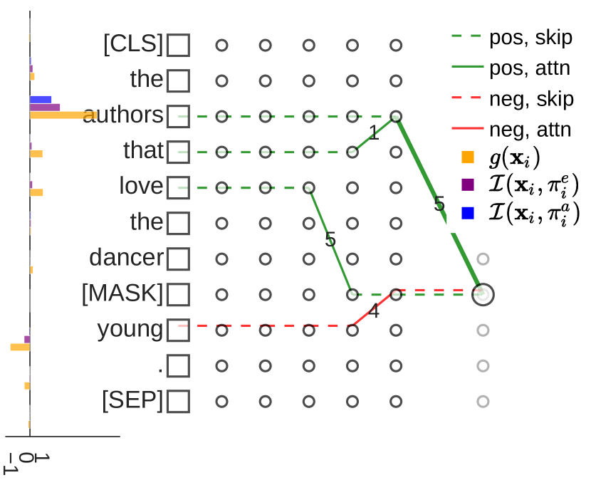
(a) SVA-Subj, PS case

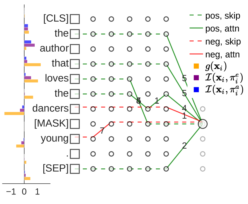
(b) SVA-Subj, SP case

Figure 6: Examples of SVA-Subj

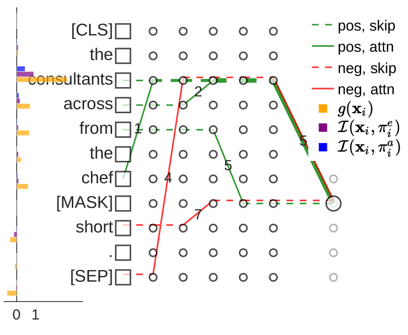
(a) SVA-APP, PS case

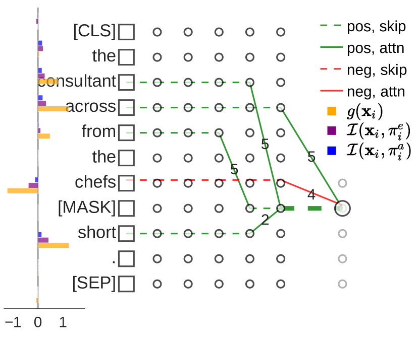
(b) SVA-APP, SP case

Figure 7: Examples of SVA-APP

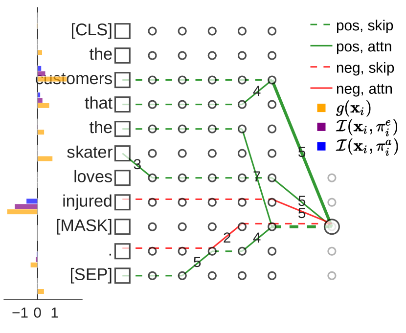
(a) RA-NA, PS case

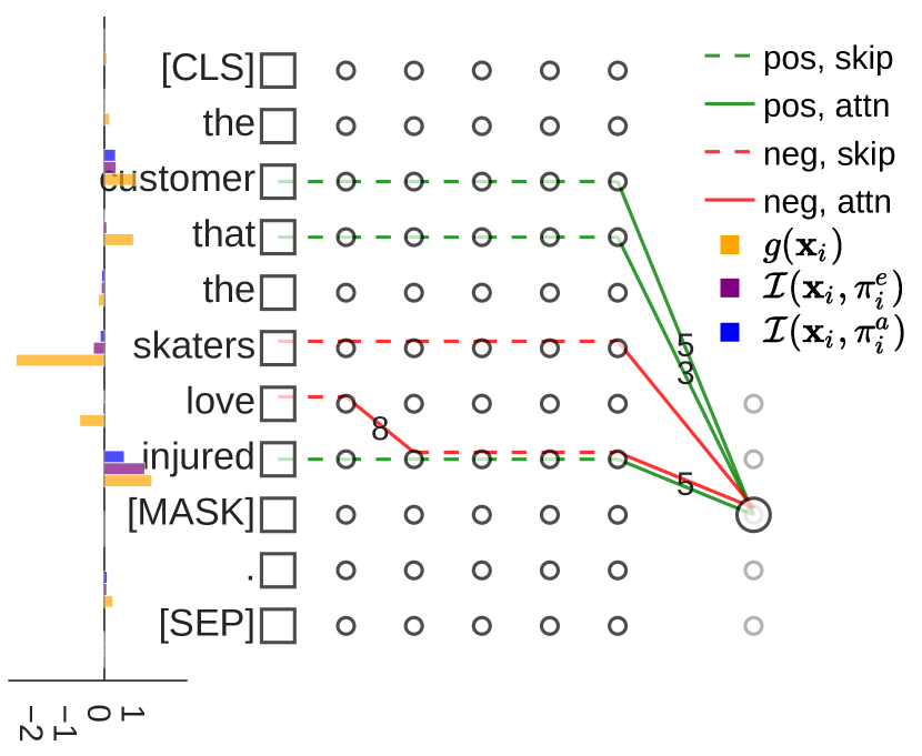
(b) RA-NA, SP case

Figure 8: Examples of RA-NA

Figure 9: Example pattern of a positive sentence in SA

Figure 10: Example pattern of a positive sentence in SA

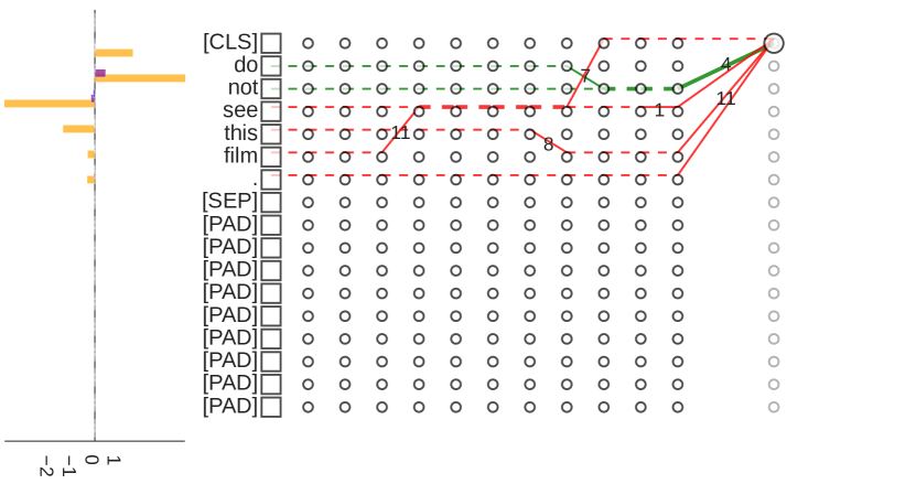
Figure 11: Example pattern of a negative sentence in SA

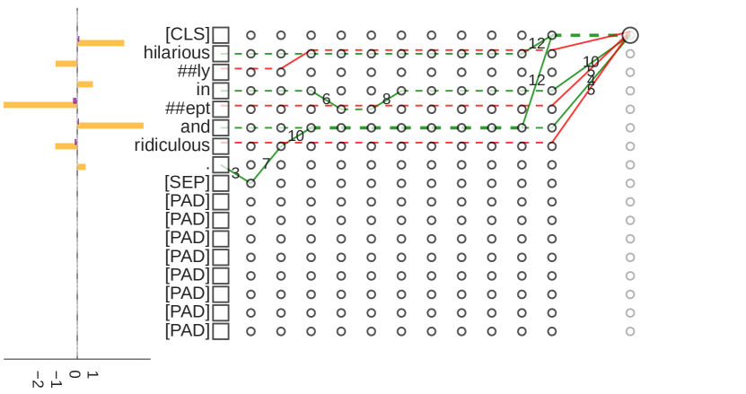
Figure 12: Example pattern of a positive sentence in SA

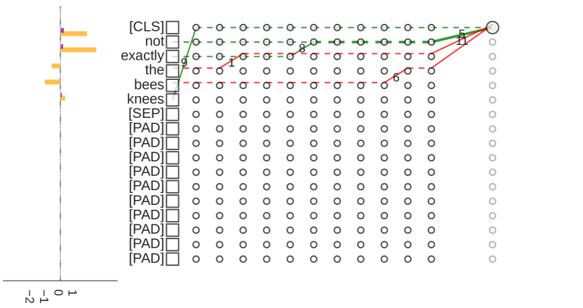
Figure 13: Example pattern of a negative sentence in SA

E.2 Aggregated Visualizations

In this section, we show the aggregated visualization(Fig. 14 and 15 ) across all examples of each case in two subtasks (SVA-Obj & NA-GA) by superimposing the patterns of individual instances (e.g. Figure 3(a) and  3(b)), while adjusting the line width to be proportional to the frequency of flow across all examples. The words within parenthesis represent one instance of the word in that position. The aggregated graphs verify (1) generality of patterns across examples in each case (including SS and PP). (2) a more intuitive visualization of the pattern entropy in these two tasks, with RA-NA showing “messier” aggregated patterns, or larger entropy.

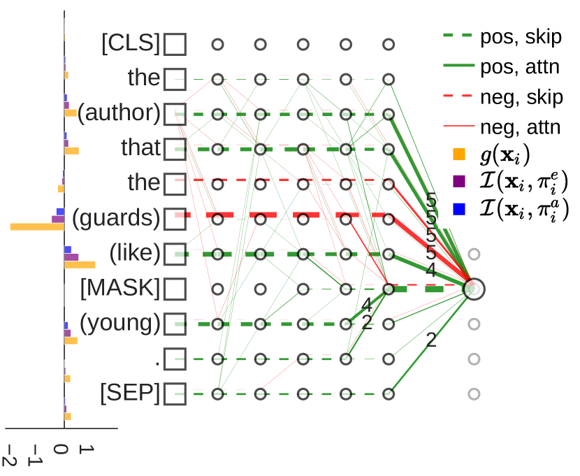
(a) singular subject + plural intervening noun(SP)

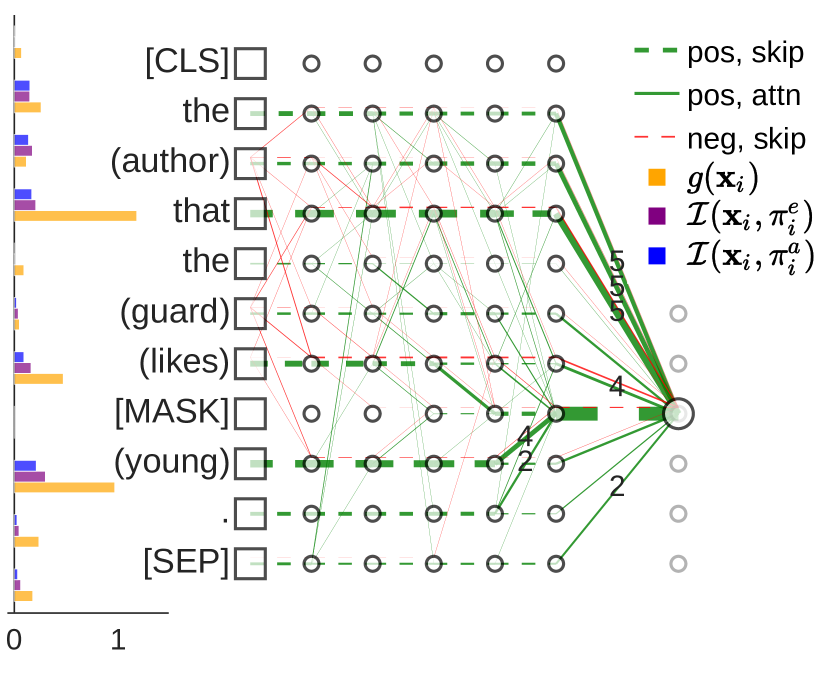
(b) singular subject + singular intervening noun(SS)

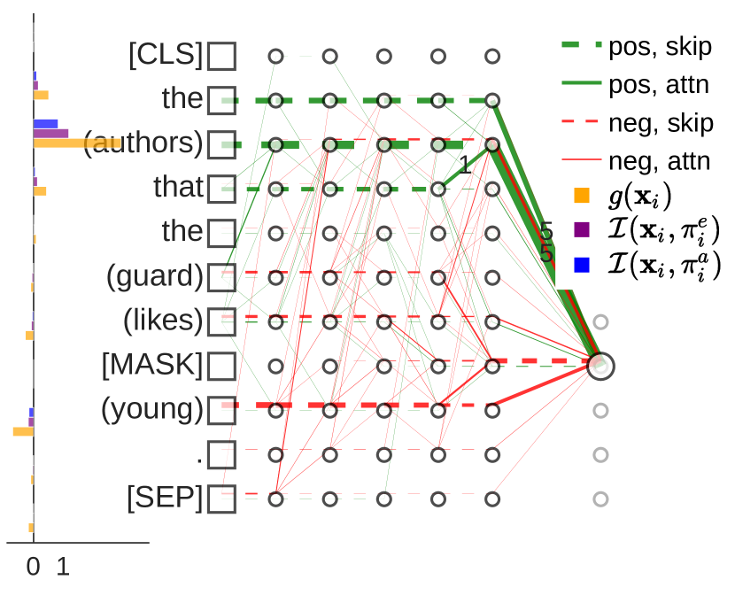
(c) plural subject + singular intervening noun(PS)

(d) plural subject + plural intervening noun(PP)

Figure 14: SVA-Obj. Aggregated

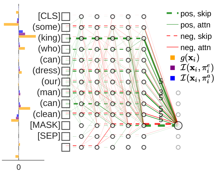
(a) male subject + male intervening noun(MM)

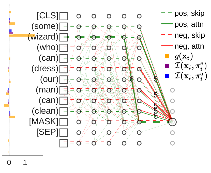
(b) female subject + male intervening noun(FM)

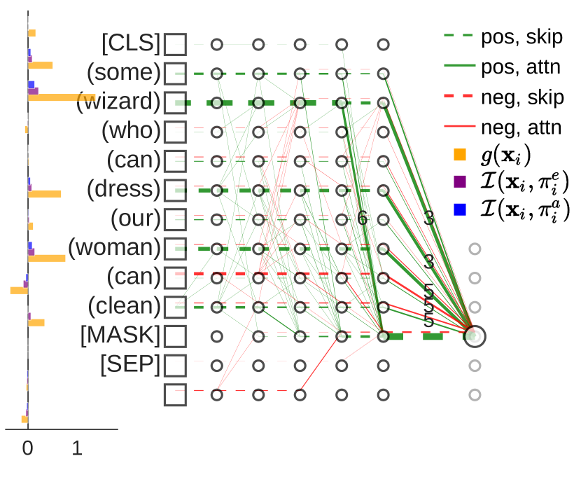
(c) female subject + female intervening noun(FF)

(d) male subject + female intervening noun(MF)

Figure 15: RA: GA, Aggregated

E.3 Impact Statement

Our work is expected to have general positive broader impacts on the uses of machine learning in the natural language processing. Specifically, we are addressing the continual lack of transparency in deep learning and the potential of intentional abuse of NLP systems employing deep learning. We hope that work such as ours will be used to build more trustworthy systems. Transparency/interpretability tools as we are building in this paper offer the ability for human users to peer inside the language models, e.g. BERT, to investigate the potential model quality issues, e.g. data bias and the abuse of privacy, which will in turn provide insights to improve the model quality. Conversely, the instrument we provide in this paper, when applied to specific realizations of language generation and understanding, can be used to scrutinize the ethics of these models’ behavior. We believe the publication of the work is more directly useful in ways positive to the broader society. As our method does not use much resources for training or building new models for applications, we believe there are no significant negative social impacts.

References

- [1] Martín Abadi, Ashish Agarwal, Paul Barham, Eugene Brevdo, Zhifeng Chen, Craig Citro, Greg S. Corrado, Andy Davis, Jeffrey Dean, Matthieu Devin, Sanjay Ghemawat, Ian Goodfellow, Andrew Harp, Geoffrey Irving, Michael Isard, Yangqing Jia, Rafal Jozefowicz, Lukasz Kaiser, Manjunath Kudlur, Josh Levenberg, Dandelion Mané, Rajat Monga, Sherry Moore, Derek Murray, Chris Olah, Mike Schuster, Jonathon Shlens, Benoit Steiner, Ilya Sutskever, Kunal Talwar, Paul Tucker, Vincent Vanhoucke, Vijay Vasudevan, Fernanda Viégas, Oriol Vinyals, Pete Warden, Martin Wattenberg, Martin Wicke, Yuan Yu, and Xiaoqiang Zheng. TensorFlow: Large-scale machine learning on heterogeneous systems, 2015. Software available from tensorflow.org.
- [2] Samira Abnar and Willem Zuidema. Quantifying attention flow in transformers. In Proceedings of the 58th Annual Meeting of the Association for Computational Linguistics, pages 4190–4197, 2020.
- [3] Marco Ancona, Enea Ceolini, Cengiz Öztireli, and Markus Gross. Towards better understanding of gradient-based attribution methods for deep neural networks. In International Conference on Learning Representations, 2018.
- [4] Gino Brunner, Yang Liu, Damian Pascual, Oliver Richter, Massimiliano Ciaramita, and Roger Wattenhofer. On identifiability in transformers. In International Conference on Learning Representations, 2020.
- [5] Kevin Clark, Urvashi Khandelwal, Omer Levy, and Christopher D Manning. What does bert look at? an analysis of bert’s attention. In Proceedings of the 2019 ACL Workshop BlackboxNLP: Analyzing and Interpreting Neural Networks for NLP, 2019.
- [6] P. Dabkowski and Yarin Gal. Real time image saliency for black box classifiers. In NIPS, 2017.
- [7] Jacob Devlin, Ming-Wei Chang, Kenton Lee, and Kristina Toutanova. Bert: Pre-training of deep bidirectional transformers for language understanding. In Proceedings of the 2019 Conference of the North American Chapter of the Association for Computational Linguistics: Human Language Technologies, Volume 1 (Long and Short Papers), pages 4171–4186, 2019.
- [8] Jay DeYoung, Sarthak Jain, Nazneen Fatema Rajani, Eric Lehman, Caiming Xiong, Richard Socher, and Byron C Wallace. Eraser: A benchmark to evaluate rationalized nlp models. Transactions of the Association for Computational Linguistics, 2020.
- [9] Kedar Dhamdhere, Mukund Sundararajan, and Qiqi Yan. How important is a neuron. In International Conference on Learning Representations, 2019.
- [10] Yihe Dong, Jean-Baptiste Cordonnier, and Andreas Loukas. Attention is not all you need: pure attention loses rank doubly exponentially with depth. In Marina Meila and Tong Zhang, editors, Proceedings of the 38th International Conference on Machine Learning, volume 139 of Proceedings of Machine Learning Research, pages 2793–2803. PMLR, 18–24 Jul 2021.
- [11] Yanai Elazar, Shauli Ravfogel, Alon Jacovi, and Yoav Goldberg. When bert forgets how to pos: Amnesic probing of linguistic properties and mlm predictions. arXiv preprint arXiv:2006.00995, 2020.
- [12] Kawin Ethayarajh and Dan Jurafsky. Attention flows are shapley value explanations. arXiv preprint arXiv:2105.14652, 2021.
- [13] Yoav Goldberg. Assessing bert’s syntactic abilities. arXiv preprint arXiv:1901.05287, 2019.
- [14] John Hewitt and Percy Liang. Designing and interpreting probes with control tasks. In Proceedings of the 2019 Conference on Empirical Methods in Natural Language Processing and the 9th International Joint Conference on Natural Language Processing (EMNLP-IJCNLP), 2019.
- [15] John Hewitt and Christopher D Manning. A structural probe for finding syntax in word representations. In Proceedings of the 2019 Conference of the North American Chapter of the Association for Computational Linguistics: Human Language Technologies, Volume 1 (Long and Short Papers), 2019.
- [16] Dieuwke Hupkes, Sara Veldhoen, and Willem Zuidema. Visualisation and’diagnostic classifiers’ reveal how recurrent and recursive neural networks process hierarchical structure. Journal of Artificial Intelligence Research, 61:907–926, 2018.
- [17] Ganesh Jawahar, Benoît Sagot, and Djamé Seddah. What does bert learn about the structure of language? In Proceedings of the 57th Annual Meeting of the Association for Computational Linguistics, 2019.
- [18] Xiaoqi Jiao, Yichun Yin, Lifeng Shang, Xin Jiang, Xiao Chen, Linlin Li, Fang Wang, and Qun Liu. Tinybert: Distilling bert for natural language understanding. arXiv preprint arXiv:1909.10351, 2019.
- [19] Jaap Jumelet, Willem Zuidema, and Dieuwke Hupkes. Analysing neural language models: Contextual decomposition reveals default reasoning in number and gender assignment. In Proceedings of the 23rd Conference on Computational Natural Language Learning (CoNLL), pages 1–11, 2019.
- [20] Josef Klafka and Allyson Ettinger. Spying on your neighbors: Fine-grained probing of contextual embeddings for information about surrounding words. In Proceedings of the 58th Annual Meeting of the Association for Computational Linguistics, 2020.
- [21] Olga Kovaleva, Alexey Romanov, Anna Rogers, and Anna Rumshisky. Revealing the dark secrets of bert. In Proceedings of the 2019 Conference on Empirical Methods in Natural Language Processing and the 9th International Joint Conference on Natural Language Processing (EMNLP-IJCNLP), pages 4365–4374, 2019.
- [22] Yair Lakretz, Germán Kruszewski, Théo Desbordes, Dieuwke Hupkes, Stanislas Dehaene, and Marco Baroni. The emergence of number and syntax units in lstm language models. In Proceedings of the 2019 Conference of the North American Chapter of the Association for Computational Linguistics: Human Language Technologies, Volume 1 (Long and Short Papers), 2019.
- [23] Klas Leino, Shayak Sen, Anupam Datta, Matt Fredrikson, and Linyi Li. Influence-directed explanations for deep convolutional networks. In 2018 IEEE International Test Conference (ITC). IEEE, 2018.
- [24] Yongjie Lin, Yi Chern Tan, and Robert Frank. Open sesame: Getting inside bert’s linguistic knowledge. In Proceedings of the 2019 ACL Workshop BlackboxNLP: Analyzing and Interpreting Neural Networks for NLP, 2019.
- [25] Tal Linzen, Emmanuel Dupoux, and Yoav Goldberg. Assessing the ability of lstms to learn syntax-sensitive dependencies. Transactions of the Association for Computational Linguistics, 2016.
- [26] Nelson F Liu, Matt Gardner, Yonatan Belinkov, Matthew E Peters, and Noah A Smith. Linguistic knowledge and transferability of contextual representations. In Proceedings of the 2019 Conference of the North American Chapter of the Association for Computational Linguistics: Human Language Technologies, 2019.
- [27] Kaiji Lu, Piotr Mardziel, Klas Leino, Matt Fredrikson, and Anupam Datta. Influence paths for characterizing subject-verb number agreement in LSTM language models. In Proceedings of the 58th Annual Meeting of the Association for Computational Linguistics. Association for Computational Linguistics, 2020.
- [28] Rebecca Marvin and Tal Linzen. Targeted syntactic evaluation of language models. In Proceedings of the 2018 Conference on Empirical Methods in Natural Language Processing, 2018.
- [29] R Thomas McCoy, Junghyun Min, and Tal Linzen. Berts of a feather do not generalize together: Large variability in generalization across models with similar test set performance. In Proceedings of the Third BlackboxNLP Workshop on Analyzing and Interpreting Neural Networks for NLP, pages 217–227, 2020.
- [30] Tom McCoy, Ellie Pavlick, and Tal Linzen. Right for the wrong reasons: Diagnosing syntactic heuristics in natural language inference. In Proceedings of the 57th Annual Meeting of the Association for Computational Linguistics, pages 3428–3448, 2019.
- [31] Paul Michel, Omer Levy, and Graham Neubig. Are sixteen heads really better than one? In Advances in Neural Information Processing Systems, 2019.
- [32] Sai Prasanna, Anna Rogers, and Anna Rumshisky. When bert plays the lottery, all tickets are winning. arXiv preprint arXiv:2005.00561, 2020.
- [33] Emily Reif, Ann Yuan, Martin Wattenberg, Fernanda B Viegas, Andy Coenen, Adam Pearce, and Been Kim. Visualizing and measuring the geometry of bert. In Advances in Neural Information Processing Systems 32. NeurIPS, 2019.
- [34] Marco Tulio Ribeiro, Tongshuang Wu, Carlos Guestrin, and Sameer Singh. Beyond accuracy: Behavioral testing of nlp models with checklist. In Proceedings of the 58th Annual Meeting of the Association for Computational Linguistics, pages 4902–4912, 2020.
- [35] Victor Sanh, Lysandre Debut, Julien Chaumond, and Thomas Wolf. Distilbert, a distilled version of bert: smaller, faster, cheaper and lighter. arXiv preprint arXiv:1910.01108, 2019.
- [36] Sofia Serrano and Noah A Smith. Is attention interpretable? In Proceedings of the 57th Annual Meeting of the Association for Computational Linguistics, 2019.
- [37] Daniel Smilkov, Nikhil Thorat, Been Kim, Fernanda Viégas, and Martin Wattenberg. Smoothgrad: removing noise by adding noise. arXiv preprint arXiv:1706.03825, 2017.
- [38] Mukund Sundararajan and Amir Najmi. The many shapley values for model explanation, 2020.
- [39] Mukund Sundararajan, Ankur Taly, and Qiqi Yan. Axiomatic attribution for deep networks. In Proceedings of the 34th International Conference on Machine Learning-Volume 70, 2017.
- [40] Ian Tenney, Dipanjan Das, and Ellie Pavlick. Bert rediscovers the classical nlp pipeline. In Proceedings of the 57th Annual Meeting of the Association for Computational Linguistics, 2019.
- [41] Ian Tenney, Patrick Xia, Berlin Chen, Alex Wang, Adam Poliak, R Thomas McCoy, Najoung Kim, Benjamin Van Durme, Samuel Bowman, Dipanjan Das, et al. What do you learn from context? probing for sentence structure in contextualized word representations. In 7th International Conference on Learning Representations, ICLR 2019, 2019.
- [42] Marcos Treviso and André FT Martins. The explanation game: Towards prediction explainability through sparse communication. In Proceedings of the Third BlackboxNLP Workshop on Analyzing and Interpreting Neural Networks for NLP, pages 107–118, 2020.
- [43] Iulia Turc, Ming-Wei Chang, Kenton Lee, and Kristina Toutanova. Well-read students learn better: On the importance of pre-training compact models. arXiv preprint arXiv:1908.08962v2, 2019.
- [44] Ashish Vaswani, Noam Shazeer, Niki Parmar, Jakob Uszkoreit, Llion Jones, Aidan N. Gomez, undefinedukasz Kaiser, and Illia Polosukhin. Attention is all you need. In Proceedings of the 31st International Conference on Neural Information Processing Systems, 2017.
- [45] Jesse Vig and Yonatan Belinkov. Analyzing the structure of attention in a transformer language model. In Proceedings of the 2019 ACL Workshop BlackboxNLP: Analyzing and Interpreting Neural Networks for NLP, 2019.
- [46] Elena Voita, David Talbot, Fedor Moiseev, Rico Sennrich, and Ivan Titov. Analyzing multi-head self-attention: Specialized heads do the heavy lifting, the rest can be pruned. In Proceedings of the 57th Annual Meeting of the Association for Computational Linguistics, 2019.
- [47] Alex Wang, Amanpreet Singh, Julian Michael, Felix Hill, Omer Levy, and Samuel Bowman. Glue: A multi-task benchmark and analysis platform for natural language understanding. In Proceedings of the 2018 EMNLP Workshop BlackboxNLP: Analyzing and Interpreting Neural Networks for NLP, pages 353–355, 2018.
- [48] Zifan Wang, Haofan Wang, Shakul Ramkumar, Matt Fredrikson, Piotr Mardziel, and Anupam Datta. Smoothed geometry for robust attribution. In Advances in Neural Information Processing Systems. NeurIPS, 2020.
- [49] Zhengxuan Wu, Thanh-Son Nguyen, and Desmond Ong. Structured self-attention weights encodes semantics in sentiment analysis. In Proceedings of the Third BlackboxNLP Workshop on Analyzing and Interpreting Neural Networks for NLP, pages 255–264, 2020.