Semi-supervised Federated Learning for Activity Recognition

Abstract.

Training deep learning models on in-home IoT sensory data is commonly used to recognise human activities. Recently, federated learning systems that use edge devices as clients to support local human activity recognition have emerged as a new paradigm to combine local (individual-level) and global (group-level) models. This approach provides better scalability and generalisability and also offers better privacy compared with the traditional centralised analysis and learning models. The assumption behind federated learning, however, relies on supervised learning on clients. This requires a large volume of labelled data, which is difficult to collect in uncontrolled IoT environments such as remote in-home monitoring.

In this paper, we propose an activity recognition system that uses semi-supervised federated learning, wherein clients conduct unsupervised learning on autoencoders with unlabelled local data to learn general representations, and a cloud server conducts supervised learning on an activity classifier with labelled data. Our experimental results show that using a long short-term memory autoencoder and a Softmax classifier, the accuracy of our proposed system is higher than that of both centralised systems and semi-supervised federated learning using data augmentation. The accuracy is also comparable to that of supervised federated learning systems. Meanwhile, we demonstrate that our system can reduce the number of needed labels and the size of local models, and has faster local activity recognition speed than supervised federated learning does.

1. Introduction

Modern smart homes are integrating more and more Internet of Things (IoT) technologies in different application scenarios. The IoT devices can collect a variety of time-series data, including ambient data such as occupancy, temperature, and brightness, and physiological data such as weight and blood pressure. With the help of machine learning (ML) algorithms, these sensory data can be used to recognise people’s activities at home. Human activity recognition (HAR) using IoT data has the promise that can significantly improve quality of life for people who require in-home care and support. For example, anomaly detection based on recognised activities can raise alerts when an individual’s health deteriorates. The alerts can then be used for early interventions  (Enshaeifar et al., 2018b; Cao et al., 2015; Queralta et al., 2019). Analysis of long-term activities can help identify behaviour changes, which can be used to support clinical decisions and healthcare plans (Enshaeifar et al., 2018a).

An architecture for HAR is to deploy devices with computational resources at the edge of networks, which is normally within people’s homes. Such “edge devices” are capable of communicating with sensory devices to collect and aggregate the sensory data, and running ML algorithms to process the in-home activity and movement data. With the help of a cloud back-end, these edge devices can form a federated learning (FL) system (McMahan et al., 2017; Yang et al., 2019; Zhao et al., 2020), which is increasingly used as a new system to learn at population-level while constructing personalised edge models for HAR. In an FL system, clients jointly train a global Deep Neural Network (DNN) model by sharing their local models with a cloud back-end. This design enables clients to use their data to contribute to the training of the model without breaching privacy. One of the assumptions behind using the canonical FL system for HAR is that data on clients are labelled with corresponding activities so that the clients can use these data to train supervised local DNN models. In HAR using IoT data, due to the large amount of time-series data that are continuously generated from different sensors, it is difficult to guarantee that end-users are capable of labelling activity data at a large scale. Thus, the availability of labelled data on clients is one of the challenges that impede the adoption of FL systems in real-world HAR applications.

Existing solutions to utilise unlabelled data in FL systems is through data augmentation (Jeong et al., 2020; Liu et al., 2020; Zhang et al., 2020). The server of an FL system keeps some labelled data and use them to train a global model through supervised learning. The clients of the system receive the global model and use it to generate pseudo labels on augmented local data. However, this approach couples the local training on clients with the specific task (i.e., labels) from the server. If a client accesses multiple FL servers for different tasks, it has to generate pseudo labels for each of them locally, which increases the cost of local training.

In centralised ML, unsupervised learning on DNN such as autoencoders (Baldi, 2011) has been widely used to learn general representations from unlabelled data. The learned representations can then be utilised to facilitate supervised learning models with labelled data. A recent study by van Berlo et al. (van Berlo et al., 2020) shows that temporal convolutional networks can be used as autoencoders to learn representations on clients of an FL system. The representations can help with training of the global supervised model of an FL system. The resulting model’s performance is comparable to that of a fully supervised algorithm. Building upon this promising result, we propose a semi-supervised FL system that realises activity recognition using time-series data at the edge, without labelled IoT sensory data on clients, and evaluate how different factors (e.g., choices of models, the number of labels, and the size of representations) affect the performance (e.g., accuracy and inference time) of the system.

In our proposed design, clients locally train autoencoders with unlabelled time-series sensory data to learn representations. These local autoencoders are then sent to a cloud server that aggregates them into a global autoencoder. The server integrates the resulting global autoencoder into the pipeline of the supervised learning process. It uses the encoder component of the global autoencoder to transform a labelled dataset into labelled representations, with which a classifier can be trained. Such a labelled dataset on the cloud back-end server can be provided by service providers without necessarily using any personal data from users (e.g., open data or data collected from laboratory trials with consents). Whenever the server selects a number of clients, both the global autoencoder and the global classifier are sent to the clients to support local activity recognition.

We evaluated our system through simulations on different HAR datasets, with different system component designs and data generation strategies. We also tested the local activity recognition part of our system on a Raspberry Pi 4 model B, which is a low-cost edge device. With the focus on HAR using time-series sensory data, we are interested in answering the research questions as follows:

• Q1. How does semi-supervised FL using autoencoders perform in comparison to supervised learning on a centralised server?

• Q2. How does semi-supervised FL using autoencoders perform in comparison to semi-supervised FL using data augmentation?

• Q3. How does semi-supervised FL using autoencoders perform in comparison to supervised FL?

• Q4. How do the key parameters of semi-supervised FL, including the number of labels on the server and the size of learned representations, affect its performance.

• Q5. How efficient is semi-supervised FL on low-cost edge devices?

Our experimental results demonstrate several key findings:

• Using long short-term memory autoencoders as local models and a Softmax classifier model as a global classifier, the accuracy of our system is higher than that of a centralised system that only conducts supervised learning in the cloud, which means that learning general representations locally improves the performance of the system.

• Our system also has higher accuracy than semi-supervised FL using data augmentation to generate pseudo labels does.

• Our system can achieve comparable accuracy to that of a supervised FL system.

• By only conducting supervised learning in the cloud, our system can significantly reduce the needed number of labels without losing much accuracy.

• By using autoencoders, our system can reduce the size of local models. This can potentially contribute to the reduction of upload traffic from the clients to the server.

• The processing time of our system when recognising activities on a low-cost edge device is acceptable for real-time applications and is significantly lower than that of supervised FL.

2. Related

As one of the key applications of IoT that can significantly improve the quality of people’s lives, HAR has attracted an enormous amount of research. Many HAR systems have been proposed to be deployed at the edge of networks, thanks to the evergrowing computational power of different types of edge devices.

2.1. HAR at the edge

In comparison to having both data and algorithms in the cloud, edge computing (Shi et al., 2016) instead deploys devices closer to end users of services, which means that data generated by the users and computation on these data can stay on the devices locally. Modern edge devices such as Intel Next Unit of Computing (NUC) (nuc, [n.d.]) and Raspberry Pi (pi, [n.d.]) are capable of running DNN models (Servia-Rodriguez et al., 2018; Chen and Ran, 2019) and providing real-time activity recognition (Liu et al., 2018; Cartas et al., 2019) from videos. Many deep learning models such as long short-term memory (LSTM) (Hochreiter and Schmidhuber, 1997; Guan and Plötz, 2017; Hammerla et al., 2016) or convolutional neural network (CNN)  (Hammerla et al., 2016) can be applied at the edge for HAR. For example, Zhang et al. (Zhang et al., 2018) proposed an HAR system that utilised both edge computing and back-end cloud computing. One implementation of this kind of HAR edge systems was proposed by Cao et al. (Cao et al., 2015), which implemented fall detection both at the edge and in the cloud. Their results show that their system has lower response latency than that of a cloud based system. Queralta et al. (Queralta et al., 2019) also proposed a fall detection system that achieved over 90% precision and recall. Uddin (Uddin, 2019) proposed a system that used more diverse body sensory data including electrocardiography (ECG), magnetometer, accelerometer, and gyroscope readings for activity recognition.

These HAR systems, however, send the personal data of their users to a back-end cloud server to train deep learning models, which poses great privacy threats to the data subjects. Servia-Rodríguez et al. (Servia-Rodriguez et al., 2018) proposed a system in which a small group of users voluntarily share their data to the cloud to train a model. Other users in the system can download this model for local training, which protects the privacy of the majority in the system but does not utilise the fine trained local models from different users to improve the performance of each other’s models. To improve the utility of local models and protect privacy at the same time, we apply federated learning (McMahan et al., 2017) to HAR at the edge, which can train a global deep learning model with constant contributions from users but does not require the users to send their personal data to the cloud.

2.2. HAR with federated learning

Federated learning (FL) (McMahan et al., 2017; Yang et al., 2019) was proposed as an alternative to traditional cloud based deep learning systems. It uses a cloud server to coordinate different clients to collaboratively train a global model. The server periodically sends the global model to a selection of clients that use their local data to update the global model. The resulting local models from the clients will be sent back to the server and be aggregated into a new global model. By this means, the global model is constantly updated using users’ personal data, without having these data in the server. Since FL was proposed, it has been widely adopted in many applications (Li et al., 2020; Yu et al., 2020) including HAR. Sozinov et al. (Sozinov et al., 2018) proposed an FL based HAR system and they demonstrated that its performance is comparable to that of its centralised counterpart, which suffers from privacy issues. Zhao et al. (Zhao et al., 2020) proposed an FL based HAR system for activity and health monitoring. Their experimental results show that, apart from acceptable accuracy, the inference time of such a system on low-cost edge devices such as Raspberry Pi is marginal. Feng et al. (Feng et al., 2020) introduced locally personalised models in FL based HAR systems to further improve the accuracy for mobility prediction. Specifically, HAR applications that need both utility and privacy guarantees such as smart healthcare can benefit from the accurate recognition and the default privacy by design of FL. For example, the system recently proposed by Chen et al. (Chen et al., 2020) applied FL to wearable healthcare, with a specific focus on the auxiliary diagnosis of Parkinson’s disease.

Existing HAR systems with canonical FL use supervised learning that relies on the assumption that all local data on clients are properly labelled with activities. This assumption is difficult to be satisfied in the scenario of IoT using sensory data. Compared to the existing FL based HAR systems, we aim to address this issue by utilising semi-supervised machine learning, which does not need locally labelled data.

2.3. Semi-supervised federated learning

Semi-supervised learning combines both supervised learning that requires labelled data and unsupervised learning that does not use labels when training DNN models. Traditional centralised ML has benefited from semi-supervised learning techniques such as transfer learning  (Khan and Roy, 2018; Zhang and Ardakanian, 2019) and autoencoders (Baldi, 2011). These techniques have been widely used in centralised ML such as learning time-series representations from videos (Srivastava et al., 2015), learning representations to compress local data (Hu and Krishnamachari, 2020), and learning representations that do not contain sensitive information (Malekzadeh et al., 2018).

The challenge of having available local labels in FL has motivated a number of systems that aim to realise FL in a semi-supervised or self-supervised fashion. The majority of the existing solutions in this area focuses on generating pseudo labels for unlabelled data and using these labels to conduct supervised learning (Jeong et al., 2020; Liu et al., 2020; Zhang et al., 2020; Long et al., 2020; Zhang et al., 2021; Kang et al., 2020; Wang et al., 2020; Yang et al., 2020). For example, Jeong et al. (Jeong et al., 2020) use data augmentation to generate fake labels and keep the consistency of the labels across different FL clients. However, the inter-client consistency requires some clients to share their data with others, which poses privacy issues. Liu et al. (Liu et al., 2020) use labelled data on an FL server to train a model through supervised learning and then send this model to FL clients to generate labels on their local data. These solutions couple the local training on clients with the specific task from the server, which means that a client has to generate pseudo labels for all the servers that have different tasks.

Another direction of semi-supervised FL is to conduct unsupervised learning on autoencoders locally on clients instead of generating pseudo labels. Compared with existing solutions, the trained autoencoders learn general representations from data, which are independent from specific tasks. Preliminary results from the work by van Berlo  et al. (van Berlo et al., 2020) show promising potential of using autoencoders to implement semi-supervised FL. Compared to their work, we evaluate different local models (i.e., autoencoders, convolutional autoencoders, and LSTM autoencoders), investigate different design considerations, and test how efficient its local activity recognition is when running on low-cost edge devices.

3. Methodology

Our goal is to implement HAR using an FL system, without having any labelled data on the edge clients. We first introduce the long short-term memory model (Hochreiter and Schmidhuber, 1997), which is a technique for analysing time-series data for HAR. We then introduce autoencoders, which are the key technique for deep unsupervised learning. We finally demonstrate the design of our proposed semi-supervised FL system and describe how unsupervised and supervised learning models are used in our framework.

3.1. Long short-term memory

The long short-term memory (LSTM) belongs to recurrent neural network (RNN) models, which are a class of DNN that processes sequences of data points such as time-series data. At each time point of the time series, the output of an RNN, which is referred to as the “hidden state”, is fed to the network together with the next data point in the time-series sequence. An RNN works in a way that, as time proceeds, it recurrently takes and processes the current input and the previous output (i.e., the hidden state), and generates a new output for the current time. Specifically for LSTM, Fig. 1 shows the network structure of a basic LSTM unit, which is called an LSTM cell. At each time $t$, it takes three input variables, which are the current observed data point $X_{t}$, the previous state of the cell $C_{t-1}$, and the previous hidden state $h_{t-1}$. For the case of applying LSTM to HAR, $X_{t}$ is a vector of all the observed sensory readings at time $t$. $h_{t}$ is the hidden state of the activity to be recognised in question.

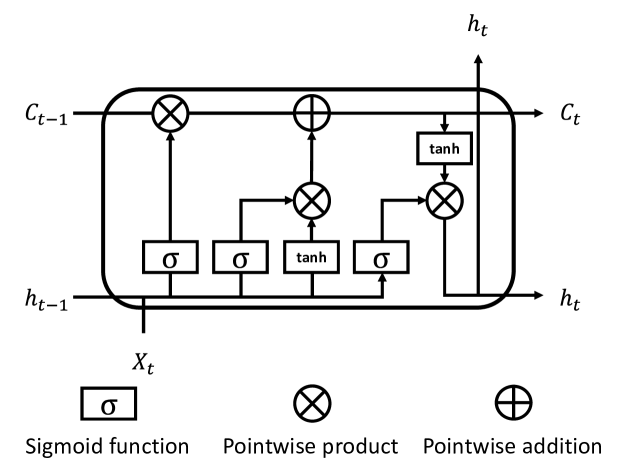
Figure 1. Network structure of a long short-term memory (LSTM) cell. At each time point $t$, the current cell state $C_{t}$ and hidden state $h_{t}$ is dependent on the previous cell state $C_{t-1}$, the previous hidden state $h_{t}$, and the current observed data point $X_{t}$.

LSTM can be used in both supervised learning and unsupervised learning. For supervised learning, each $X_{t}$ of a time-series sequence has a corresponding label $Y_{t}$ (e.g., activity class at time point $t$) as the ground truth. The hidden state $h_{t}$ can be fed into a “Softmax classifier” that contains a fully-connected layer and a Softmax layer. By this means, such an LSTM classifier can be trained against the labelled activities through feedforward and backpropagation to minimise the loss (e.g., Cross-entropy loss) between the classifications and the ground truth. For unsupervised learning, LSTM can be trained as components of an autoencoder, which we will describe in detail in Sec. 3.2.

3.2. Autoencoder

An autoencoder (Baldi, 2011) is a type of neural network that is used to learn latent feature representations from data. Different from supervised learning that aims to learn a function $f(X)\rightarrow Y$ from input variables $X$ to labels $Y$, an autoencoder used in unsupervised learning tries to encode $X$ to its latent representation $h$ and to decode $h$ into a reconstruction of $X$, which is presented as $X^{\prime}$. Fig. 2 demonstrates two types of autoencoders that use different neural networks. The simple autoencoder in Fig. LABEL:sub@sub_fig:ae uses fully connected layers to encode $X$ into $h$ and then to decode $h$ into $X^{\prime}$. The convolutional autoencoder in Fig. LABEL:sub@sub_fig:cae uses a convolutional layer that moves small kernels alongside the input $X$ and conducts convolution operations on each part of $X$ to encode it into $h$. The decoder part uses a transposed convolutional layer that moves small kernels on $h$ to upsample it into $X^{\prime}$.

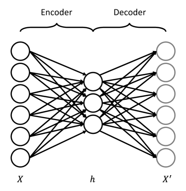
(a)

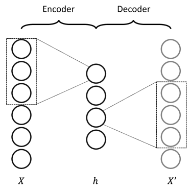
(b)

Figure 2. Network structures of a simple autoencoder and a convolutional autoencoder. The encoder part compresses the input $X$ into a representation $h$ that has fewer dimensions. The decoder part tries to generate a reconstruction $X^{\prime}$ from $h$, which is supposed to be close to $X$.

Ideally, $X^{\prime}$ is supposed to be as close to $X$ as possible, based on the assumption that the key representations of $X$ can be learned and encoded as $h$. As the dimensionality of $h$ is lower than that of $X$, there is less information in $h$ than in $X$. Thus the reconstructed $X^{\prime}$ is likely to be a distorted version of $X$. The goal of training an autoencoder is to minimise the distortion, i.e., minimising a loss function $L(X,X^{\prime})$, thereby producing an encoder (e.g., fully connected hidden layers or convolutional hidden layers) that can capture $X$’s most useful information in its representation $h$.

As mentioned Sec. 3.1, LSTM can also be used as components of an LSTM-autoencoder (Srivastava et al., 2015) to encode time-series data. As shown in Fig. 3, an LSTM cell is used as the encoder of an autoencoder and takes a time-series sequence as its input. The final hidden state $h_{3}$ is the representation of $X_{3}$ in the context of the sequence $(X_{1},X_{2},X_{3})$. As the hidden state of the LSTM encoder is based on both the input observation and the previous hidden states, the representation generated in this way compresses information of both the features in the observation and the time-series sequence. The decoder, which is another LSTM cell, reconstructs the original sequence in a reversed order. Thus, the goal of an LSTM-autoencoder is to minimise the loss between the original and the reconstructed sequences.

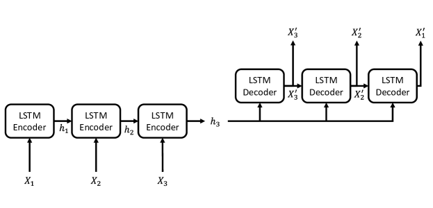
Figure 3. Network structure of an LSTM-autoencoder. The time-series sequence $(X_{1},X_{2},X_{3})$ is input into an LSTM encoder cell and the final output hidden state $h_{3}$ (i.e., after $X_{3}$ is input into the encoder) is the representation of $X_{3}$ in the context of $(X_{1},X_{2},X_{3})$. A sequence of the learned representation with the same length as that of the original sequence, i.e., $(h_{3},h_{3},h_{3})$, is input into an LSTM decoder cell. The output sequence tries to reconstruct the original sequence in reversed order.

Since our system runs unsupervised learning locally at the edge and supervised learning in the cloud, we consider simple autoencoders, convolutional autoencoders, and LSTM-autoencoders in our proposed system, in order to understand how the location where time-series information is captured (i.e., in supervised learning or unsupervised learning) affect the performance of our system.

3.3. System design

In a canonical FL system, as in a client-server structure, a cloud server periodically sends a global model to selected clients for updating the model locally. As shown in Fig. 4, in each communication round $t$, a global model $w^{g}_{t}$ is sent to three selected clients, which conduct supervised learning on $w^{g}_{t}$ with their labelled local data. The resulting local models are then sent to the server, which uses the federated averaging (FedAvg) algorithm (McMahan et al., 2017) to aggregate these models into a new global model $w^{g}_{t+1}$. The server and clients repeat this procedure through multiple communication rounds between them, thereby fitting the global model to clients’ local data without releasing the data to the server.

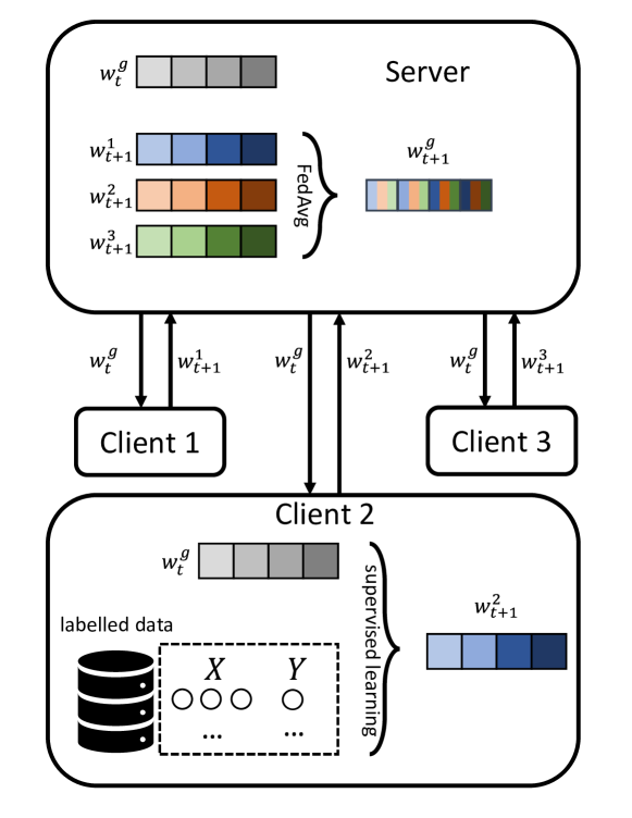
Figure 4. System structure of a canonical federated learning (FL) system with supervised learning. The server selects 3 clients and sends the global $w^{g}_{t}$ to them and the clients use their labelled data to update $w^{g}_{t}$ into their local models, which are then sent to the server to be aggregated into a new global model using the FedAvg algorithm.

In order to address the lack of labels on clients in HAR with IoT sensory data, our proposed system applies semi-supervised learning in an FL system, in which clients use unsupervised learning to train autoencoders with their unlabelled data, and a server uses supervised learning to train a classifier that can map encoded representations to activities with a labelled dataset.

As shown in Fig. 5, in each communication round, the server sends a global autoencoder $w^{a_{g}}_{t}$ to selected clients. In order to update $w^{a_{g}}_{t}$ locally, clients run unsupervised learning on $w^{a_{g}}_{t}$ with their unlabelled local data and then send the resulting local autoencoders to the server. The server follows the standard FedAvg algorithm to generate a new global autoencoder $w^{a_{g}}_{t+1}$, which is then plugged into the pipeline of supervised learning with a labelled dataset $D=(X,Y)$. The server first uses the encoder part of $w^{a_{g}}_{t+1}$ to encode the original features $X$ into representations $X^{\prime}$ in order to generate a labelled representation dataset $D^{\prime}=(X^{\prime},Y)$. Then the server conducts supervised learning with $D^{\prime}$ to update a classifier $w^{s}_{t}$ into $w^{s}_{t+1}$. Fig. 6 shows the detailed semi-supervised algorithm of our system.

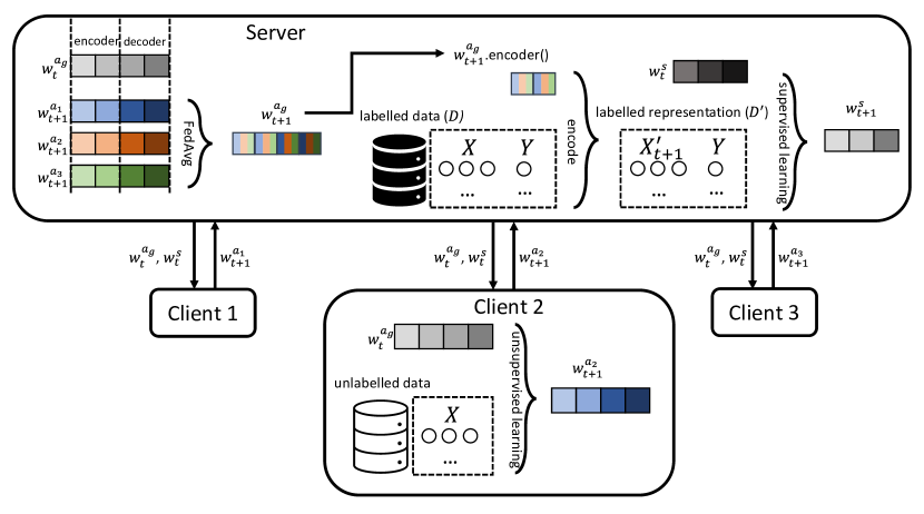
Figure 5. System structure of our semi-supervised FL system. A server and three clients follow the standard FL procedure to update a global autoencoder $w^{a_{g}}_{t}$ to $w^{a_{g}}_{t+1}$. Then the server uses the encoder of $w^{a_{g}}_{t+1}$ to encode the labelled dataset $D$ on the server into a labelled representation dataset $D^{\prime}$. It then conducts supervised learning on a classifier $w^{s}_{t}$ with $D^{\prime}$ and generates a new classifier $w^{s}_{t+1}$.

 

1:$K$: number of clients; $C$: fraction of clients; $D=(X,Y)$: labelled dataset in the format as $(features,label)$

2:initialises $w^{a_{g}}_{0}$, $w^{s}_{0}$ at $t=0$

3:for all communication round $t$ do $S_{t}\leftarrow$ randomly selected $K\cdot C$ clients

4:     for all client $k\in S_{t}$ do

5:         $w_{t+1}^{a_{k}}\leftarrow LocalTraining(k,w^{a_{g}}_{t})$ $\triangleright$ on client $k$

6:     end for

7:     $w^{a_{g}}_{t+1}\leftarrow\displaystyle\sum_{k\in S_{t}}\frac{n_{k}}{n}w^{a_{k}}_{t+1}$ $\triangleright$ FedAvg on the server

8:     $X^{\prime}\leftarrow w^{a_{g}}_{t+1}.encoder(X)$

9:     $D^{\prime}_{t}\leftarrow(X^{\prime},Y)$

10:     $w^{s}_{t+1}\leftarrow CloudTraining(D^{\prime}_{t},w^{s}_{t})$ $\triangleright$ on the server

11:end for  

Figure 6. Algorithm of semi-supervised FL. $n_{k}$ and $n$ are the numbers of unlabelled samples on client $k$ and on all selected clients, respectively. $LocalTraining$ is unsupervised learning on the global autoencoder $w^{a_{g}}_{t}$ on a client. $CloudTraining$ is supervised learning on the classifier $w^{s}_{t}$ on the server.

In each communication round $t$, the resulting classifier $w^{s}_{t}$ is also sent to selected clients with the global autoencoder $w^{g_{a}}_{t}$. In order to locally recognise activities from its observations $X$, a client first uses the encoder part of $w^{g_{a}}_{t}$ to transform $X$ into its presentation $X^{\prime}$, and then feeds $X^{\prime}$ into the classifier $w^{s}_{t}$ to recognise the corresponding activities.

4. Evaluation

We evaluated our system through simulations on different human activity datasets with different system designs and configurations. In addition we evaluated the local activity recognition algorithms of our system on a Raspberry Pi 4 model B. We want to answer research questions as follow:

• Q1. How does our system perform in comparison to supervised learning on a centralised server?

• Q2. How does our system perform in comparison to semi-supervised FL using data augmentation?

• Q3. How does our system perform in comparison to supervised FL?

• Q4. How do the key parameters of our system, including the size of labelled samples on the server and the size of learned representations, affect the performance of HAR.

• Q5. How efficient is semi-supervised FL on low-cost edge devices.

4.1. Datasets

We used three HAR datasets that contain time-series sensory data in our evaluation. The datasets have different numbers of features and activities with different durations and frequencies.

The Opportunity (Opp) dataset (Chavarriaga et al., 2013) contains short-term and non-repeated kitchen activities of 4 participants. The Daphnet Freezing of Gait (DG) dataset (Bachlin et al., 2009) contains Parkinson’s Disease patients’ freezing of gaits incidents collected from 10 participants, which are also short-term and non-repeated. The PAMAP2 dataset (Reiss and Stricker, 2012) contains household and exercise activities collected from 9 participants, which are long-term and repeated. The data pre-processing procedure in our evaluation is the same as described by Hammerla et al. (Hammerla et al., 2016). Table 1 shows detailed information about the used datasets after being pre-processed.

Table 1. HAR datasets in our experiments.

Dataset	Activities	Features	Classes	Train	Test
Opp	Kitchen	79	18	651k	119k
DG	Gait	9	3	792k	81k
PAMAP2	Household & Exercise	52	12	473k	83k

4.2. Simulation setup

We simulated a semi-supervised FL that runs unsupervised learning on 100 clients to locally update autoencoders and runs supervised learning on a server to update a classifier. In each communication round $t$, the server selects $100\cdot C$ clients to participate in the unsupervised learning, and $C$ is the fraction of clients to be selected. Each selected client uses its local data to train the global autoencoder $w^{a_{g}}_{t}$ with a learning rate $lr_{a}$ for $e_{a}$ epochs. The server conducts supervised learning to train the classifier $w^{s}_{t}$ with a learning rate $lr_{s}$ for $e_{s}$ epochs. For each individual simulation setup, we conducted 64 replicates with different random seeds.

Based on the assumption that a server is more computationally powerful than a client in practice, we set the learning rates $lr_{a}$ and $lr_{s}$ as 0.01 and 0.001, respectively. Similarly, we set the numbers of epochs $e_{a}$ and $e_{s}$ as 2 and 5, because an individual client is only supposed to run a small number of epochs of unsupervised learning and a server is capable of doing more epochs of supervised learning. The reason for setting $e_{s}=5$ is to keep the execution time of our simulation in an acceptable range. Nevertheless, we believe that this parameter on the server can be set as a larger number in real-world applications where more powerful clusters and graphics processing units (GPUs) can be deployed to accelerate the convergence of performance.

4.2.1. Baselines

To answer Q1 and Q2, we consider two baselines to 1) evaluate whether the autoencoders in our system improve the performance of the system and 2) compare the performance of our system to that of data augmentation based semi-supervised FL.

Since we assume that labelled data exist on the server of the system, thus for ablation studies, we consider a baseline system that only uses these labelled data to conduct supervised learning on the server and sends trained models to clients for local activity recognition. This system trains an LSTM classifier on labelled data on the server and does not train any autoencoders on clients. We refer to this baseline of a centralised system as CS. Comparing the performance of CS to that of our proposed system will indicate whether the autoencoders in our system have any effectiveness in improving the performance of the trained model.

To compare our system with the state of the art, we consider a semi-supervised FL system that uses data augmentation to generate pseudo labels as another baseline. We refer to this baseline as DA. It first conducts supervise learning on labelled data on the server to train an LSTM classifier. It then follows standard FL protocols to sends the trained global model to clients. Each client uses the received model to generate pseudo labels on their unlabelled local data. To introduce randomness in data augmentation, we feed sequences with randomised lengths into the model when generating labels. The sequences are then paired with the labels that are generated from them as a pseudo-labelled local dataset, which is used for locally updating the global model.

4.2.2. Autoencoders and classifiers

We implement three schemes for our system with different autoencoders, including simple autoencoders, convolutional autoencoders, and LSTM-autoencoders.

The first scheme uses a simple autoencoder with fully connected (FC) layers to learn representations from individual samples in unsupervised learning and uses a classifier that has an LSTM cell with its output hidden states connected to an FC layer and a Softmax layer, which we refer to as FC-LSTM.

The second scheme uses 1-d convolutional and transposed convolutional layers in its autoencoder. The convolutional layer has 8 output channels with kernel size 3 and has both stride and padding sizes equal to 1. The output is batch normalised and then fed into a ReLU layer. To control the size of the encoded $h$, after the ReLU layer, we flatten the output of 8 channels and feed it into a fully connected layer that transforms it into the $h$ with a specific size. For the decoder part, we have a fully connected layer whose output is unflattened into 8 channels. Then we use a 1-d transposed convolutional layer that has 1 output channel with kernel size 3 and has both stride and padding sizes equal to 1, to generate the decoded $X^{\prime}$. The LSTM classifier of this scheme has the same structure as that in FC+LSTM. We refer to this scheme as CNN-LSTM.

For the third scheme, we use an LSTM-autoencoder to capture time-series information in local unsupervised learning. Both the encoder and the decoder have 1 LSTM cell. It uses a Softmax classifier that has a fully connected layer and a Softmax layer. We refer to this scheme as LSTM-FC

For the LSTM classifiers in our experiments, we adopted the bagging (i.e., bootstrap aggregating) strategy similar to Guan and Plötz (Guan and Plötz, 2017) to train our models with random batch sizes and sequence lengths. In all schemes, we used the mean square error (MSE) loss function for autoencoders and the cross-entropy loss function for classifiers. We used the Adam optimiser in the training of all models. All the deep learning components in our simulations were implemented using PyTorch libraries (Paszke et al., 2019).

4.2.3. Label ratio and compression ratio

We adjusted two parameters to control the amount of labelled data and the size of representations. For an original training dataset that has $N^{l}$ time-series samples with labels, we adjusted the label ratio $r^{l}\in(0,1)$ and took $r^{l}\cdot N^{l}$ samples from it as the labelled training dataset on the server. Since the samples are formed as time-series sequences, to avoid breaking the activities by directly taking random samples from the sequences, we first divided the entire training set into 100 divisions. We then randomly sampled $100\cdot r^{l}$ divisions and concatenated them as the labelled training dataset on the server. For a training dataset whose observations have $N^{f}$ features, we adjusted the compression ratio $r^{f}\in(0,1)$ and used the rounded value of $r^{f}\cdot N^{f}$ as the size of the representation when training autoencoders.

4.2.4. IID and Non-IID local data

We used two strategies to generate local training data for clients from training datasets. In both strategies, the number of allocated samples for each client, i.e., $n_{k}$, equals to $\frac{n^{o}}{n^{p}}$, where $n^{o}$ is the number of samples in the original training dataset shown in Table 1 and $n^{p}$ is the number of participants (e.g., 4 for the Opp dataset) of the original dataset.

To generate IID local training datasets, we divided the training dataset into 100 divisions. For a client to be allocated $n_{k}$ samples, its local training data evenly distribute in these divisions. In each division, a time window that contains $\frac{n_{k}}{100}$ continuous samples is randomly selected, without their labels, as the client’s sample fragment in this division. The sample fragments from all divisions are then concatenated as the local training dataset for the client in the IID scenario.

For Non-IID local training datasets, we randomly located a time window with length $n_{k}$ in the training dataset and used the samples without labels in the time window as the local training dataset for the client in the Non-IID scenario. By this means, the local training dataset of each client can only represent the distribution within a single part in the unlabelled dataset.

4.3. Edge device setup

Apart from simulations, to answer Q5, we evaluated the local activity recognition part of our system on a Raspberry Pi 4 Model B. The specifications of the device are shown in Table. 2.

Table 2. System specifications of Raspberry Pi 4 Model B.

CPU	Quad core Cortex-A72 (ARM v8) 64-bit SoC @ 1.5GHz
RAM	4GB LPDDR4-3200 SDRAM
Storage	SanDisk Ultra 32GB microSDHC Memory Card
OS	Ubuntu Server 19.10

Compared with supervised FL, on the one hand, our system introduces local autoencoders that encode samples into representations before feeding them into classifiers, which costs additional processing time. On the other hand, encoded representations have smaller sizes than original samples do, which reduces the processing time of classifiers. To understand how these two factors affect the overall local processing time, we tested both supervised FL and our system on the Raspberry Pi and compared their performances. We divided the testing datasets into one-second-long sequences and measured the overall processing time of the trained models (i.e., autoencoders + classifiers) on each sequence, in order to calculate the overhead for each one-second time window.

4.4. Metrics

We evaluated the performance of the global autoencoder and the classifier with the testing datasets at the end of every other communication round. We first used a time window to select 5000 samples each time. As the sampling frequency in the processed datasets is approximately $33Hz$, this time window represents activities in about 2.53 minutes. We then applied the global autoencoder on the samples in the time window to encode them into a sequence of labelled representations. The classifier was applied to the sequence of representations to recognise the activities, which were then compared with the ground truth labels. We calculate the accuracy in the time window, which is the fraction of correctly classified representations among all representations. The accuracies from different time windows are averaged as the accuracy of the system. In every other communication round $t$, we calculate the average value from 64 simulation replicates and its standard error.

5. Results

We find that our proposed semi-supervised FL system has higher accuracy than the centralised system that only conducts supervised learning on the server. The accuracy is also higher than that of data augmentation based semi-supervised FL and is comparable to that of supervised FL that requires more labelled data and bigger local models. In addition, it has marginal local activity recognition time on a low-cost edge device.

5.1. Analysis of autoencoders and classifiers

We first look at the contribution of the autoencoders in our proposed system. As in our assumption, the server has some labelled data that can be used for supervised learning. If the server has enough labelled data to train a decent model, its accuracy may be higher than that of a semi-supervised FL. Thus the centralised system (CS) is a natural baseline that our system needs to surpass.

We adjust the label ratio $r^{l}$ from $1/2$ to $1/32$ in ablation studies for each scheme and try to find out if our system has higher accuracy than CS. We find that the scheme FC-LSTM (i.e., using simple autoencoders and LSTM classifiers) has lower accuracy than the CS baseline does under all circumstances. Therefore we remove it from our analysis. For the other schemes, we keep two $r^{l}$ values that lead to the two highest accuracies that are higher than that of the CS baseline on each dataset. Thus on the Opp dataset, our schemes have better performance than the CS baseline does when $r^{l}=\{1/16,1/32\}$. On the DG and PAMAP2 datasets, we have $r^{l}=\{1/2,1/4\}$. We test our schemes on both IID and Non-IID data but have not found significant differences in the accuracy because our schemes do not use any labels locally. Thus we only show the results on IID data. All schemes’ accuracy converges after 50 communication rounds and we only show the results during this period.

5.1.1. Ablation study of CNN autoencoder

Fig. 7 shows the accuracy of the scheme CNN+LSTM and the scheme CS, with $r^{f}=1/2$ on different datasets. As the round of communications increases, the accuracy of all schemes goes up and converges. The converged accuracy of CNN+LSTM schemes, i.e., using a convolutional autoencoder to learn representations locally and using an LSTM classifier for supervised learning in the cloud, is higher than that of the CS schemes that only conduct supervised learning in the cloud. This means that training CNN autoencoders locally indeed contributes to improving the accuracy of the system. When $r^{l}$ decreases, the converged accuracy of CNN+LSTM goes down on all datasets, which means that it is sensitive to the change of label ratios.

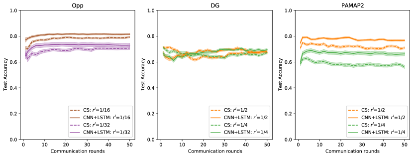
Figure 7. Test accuracy of CNN autoencoders with LSTM classifiers (CNN+LSTM), and a centralised system (CS) using LSTM classifiers without autoencoders. $r^{f}=1/2$ for both schemes. CNN+LSTM has higher converged accuracy than CS, which means that unsupervised learning on CNN autoencoders helps improve the performance.

5.1.2. Ablation study of LSTM autoencoder

Fig. 8 shows the accuracy of the scheme LSTM+FC and the scheme CS, with $r^{f}=1/2$. It demonstrates similar trends as Fig. 7 does. The accuracy of LSTM+FC, i.e., using LSTM autoencoders locally and using Softmax classifiers for supervised learning in the cloud, is higher than that of CS that runs centralised and supervised learning without using unlabelled local data. However, LSTM+FC is less sensitive to the change of label ratios. For example, its converged accuracy on the Opp dataset is almost the same when we change $r^{l}$ from $1/16$ to $1/32$. This would enable us to achieve similar performance but require fewer labelled data compared to CNN+LSTM.

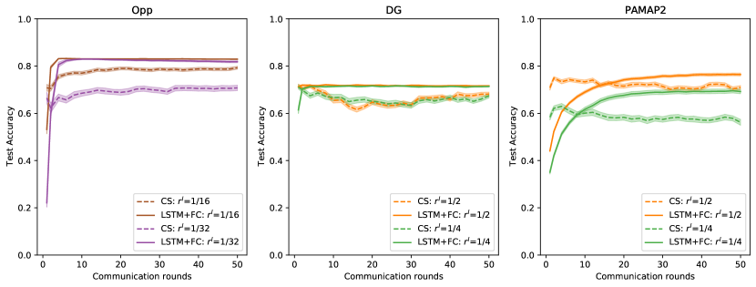
Figure 8. Test accuracy of LSTM autoencoders with Softmax classifiers (LSTM+FC), and a centralised system (CS) using LSTM classifiers without autoencoders. $r^{f}=1/2$ for both schemes. LSTM+FC has higher converged accuracy than CS. It is less sensitive to the change of $r^{l}$ than CNN+LSTM on the Opp and DG datasets.

The experimental results show that, when implementing a semi-supervised FL system for HAR, both CNN autoencoders and LSTM autoencoders can improve the accuracy of the system. Using LSTM autoencoders is less sensitive to the change of available labelled data in the cloud. In the rest of our analyses of our results, we only show the accuracy of the LSTM+FC scheme.

5.2. Comparison with different FL schemes

We now analyse the performance of our system in comparison with semi-supervised FL using data augmentation (DA) to generate pseudo labels and supervised FL having labelled data available on clients.

5.2.1. Comparison with DA

Fig. 9 shows the accuracy of both LSTM+FC and DA on three datasets. On the Opp and DG datasets, the accuracy of DA increases more slowly than LSTM+FC does. But once the accuracy of both schemes converge, they do not show significant differences. On the PAMAP2 dataset, the converged accuracy of LSTM+FC is higher than that of DA. We also find that, although the accuracy of DA on the Opp and DG datasets is higher than that of CS in Fig. 8, its accuracy on the PAMAP2 dataset in Fig. 9 converges more slowly than CS does in Fig. 8. This indicates that using the received global LSTM model to generate pseudo labels and then training the model on these pseudo labels may damage the testing accuracy. Although we used time-series sequences with randomised lengths to generate pseudo labels in our experiments, DA may still risk overfitting the model to the training data and consequently has slower speed to achieve decent accuracy on testing data.

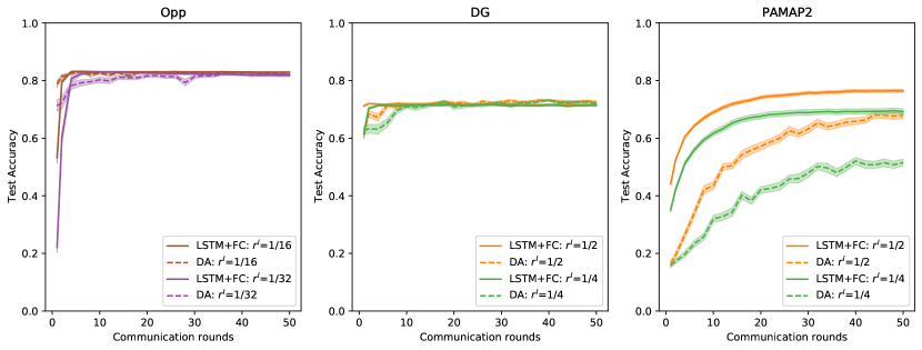
Figure 9. Test accuracy of LSTM autoencoders with Softmax classifiers (LSTM+FC), and semi-supervised FL using data augmentation (DA). There is not significant difference between their converged accuracy on the Opp and DG datasets. LSTM+FC has higher converged accuracy than DA on the PAMAP2 dataset.

Our results indicate that, for semi-supervised FL, using locally trained autoencoders can achieve higher converged accuracy than using data augmentation to generate pseudo labels. In addition, compared with DA, our scheme is independent from the specific tasks provided by the server. For example, if one client uses its unlabelled data to access multiple FL servers that conduct different tasks, with data augmentation, the client has to generate pseudo labels for each of models of these tasks. In our scheme, the client only conducts unsupervised learning locally using unlabelled data to learn general representations, which is independent from the labels in the cloud.

5.2.2. Comparison with supervised FL

Fig. 10 shows the accuracy of LSTM+FC with $r^{f}=1/2$ and a supervised FL scheme. The supervised FL uses all the information (i.e., 100% features and 100% labels) in the training datasets. Therefore it has higher accuracy than that of LSTM+FC. However, our scheme enables a trade-off between the performance of the system (i.e., accuracy), the cost of data annotation (i.e., label ratio), and the size of models (i.e., compression ratio). For example, having larger compression ratio $r^{f}=3/4$ on the PAMAP2 dataset can lead to a higher accuracy (shown in Fig. 11) that is comparable to that of the supervised FL.

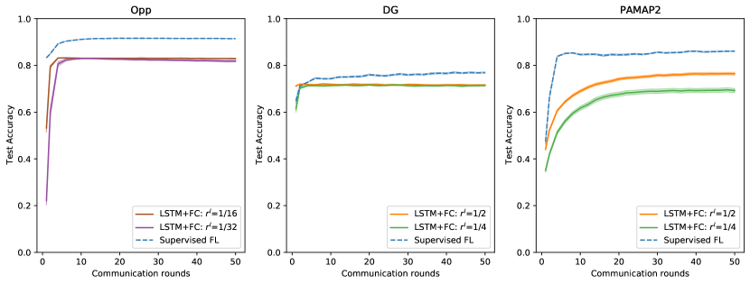
Figure 10. Test accuracy of LSTM autoencoders with Softmax classifiers (LSTM+FC, $r^{f}=1/2$), and supervised FL using 100% features and labels. The converged accuracy of LSTM+FC is comparable to that of the supervised FL and requires fewer labelled data.

The experimental results suggest that we can implement FL systems in a semi-supervised fashion with fewer needed labels than those in supervised FL, meanwhile achieve comparable accuracy. Although one of the motivations of FL is to hold models instead of personal data in the cloud to address potential privacy issues, the data held by the server of our system do not have to be from the users of the service of the system. This kind of dataset in the cloud has been used in FL to address other challenges such as dealing with Non-IID data by creating a small globally shared dataset  (Kairouz et al., 2019) and does not necessarily contain private information. We believe that service providers can collect these data from open datasets, or from laboratory trials in controlled environment where data subjects give their consents to contribute their data.

5.3. Analysis of compression ratio

We also investigate how the compression ratio $r^{f}$ of autoencoders affects the accuracy of our system. It is an important factor that can affect the number of parameters and the size of local models. These local models are regularly uploaded from the clients to the server over network, hence their sizes affect the outbound traffic. We use $r^{f}=\{3/4,1/2,1/4,1/8\}$ on all datasets. We keep $r^{l}=1/16$ for the Opp dataset and $r^{l}=1/2$ for both the DG and PAMAP2 datasets.

Fig. 11 demonstrates that, on the Opp and the DG datasets, our system can compress an original sample into a representation whose size is only $1/4$ of the original sample without significantly affecting the accuracy. On the PAMAP2 dataset, increasing $r^{f}$ from $1/2$ to $3/4$ can lead to accuracy that is comparable to that of the supervised FL scheme.

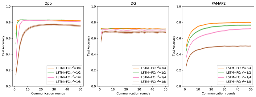
Figure 11. Test accuracy with different compression ratios $r^{f}=\{3/4,1/2,1/4,1/8\}$. $r^{l}=1/16$ for OPP and $r^{l}=1/2$ for both DG and PAMAP2. The accuracy on OPP and DG is not affected much when changing $r^{f}$ from $3/4$ to $1/4$. PAMAP2 is more sensitive to the change of $r^{f}$ than the other two datasets.

Changing the compression ratio in our system allows us to exchange accuracy with model sizes, or vice versa. When used data are not sensitive to the compression ratio (e.g., Opp and DG), compressing samples into smaller representations may significantly reduce the size of local models that are uploaded from the clients to the server, which may lead to lower network traffic.

5.4. Running time at the edge

We evaluated the local activity recognition using both supervised FL and our system (LSTM+FC) with $r^{f}=0.5$ on a Raspberry Pi. As shown in Fig. 12, the processing time of our system is significantly lower ($p<0.001$) than that of supervised FL on all datasets. Although the autoencoder in our system inevitably causes extra processing time as it increases the length of the local pipeline, the LSTM cell in the autoencoder encodes the input data into smaller representations. In contrast, the LSTM classifier in the supervised FL transforms input data into hidden states that have larger sizes. This reduction of the amount of data leads to a shorter overall processing time than that of the supervised FL.

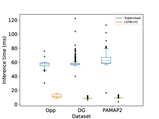
Figure 12. Local running time on a Raspberry Pi 4 Model B. Dashed lines are average values. Each data point is the processing time when recognising activities of a one-second long sequence. The running time of our system on all three datasets is significantly ($p<0.001$) lower than that of the supervised FL.

Combined with the results of Sec. 5.3, our experimental results show that running unsupervised learning on autoencoders can reduce both the size of local models and the size of data processed by classifiers. This can potentially improve not only the outbound network traffic, but also the efficiency of local activity recognition.

6. Discussion

Our experimental results show that HAR with semi-supervised FL can achieve comparable accuracy to that of supervised FL. We now discuss how these results can contribute to the system design of FL systems and possible research topics.

6.1. FL servers can do more than FedAvg

In canonical FL systems, servers only hold global models and use the FedAvg algorithm to aggregate received local models into new global models. This design consideration is due to the privacy concerns of having personal data on the servers. Our findings suggest that running supervised learning with a small amount of labelled data on the servers can alleviate individual users from labelling their local data. Therefore, we suggest that FL systems may consider maintaining datasets that do not contain private information on their servers to support semi-supervised learning. Apart from implementing the FedAvg algorithm in every communication round, servers can conduct more epochs of supervised learning than individual clients can do, since they have more computational resources and fewer power constrains than clients do. This can help the performance of the models converge faster.

6.2. Learning useful representations, not bias

By training autoencoders locally, semi-supervised FL is not affected by Non-IID data because it does not use any labels locally. This sheds light on a new solution, which is different from data augmentation or limiting individual contributions from clients (Kairouz et al., 2019), to address the Non-IID data issue in FL. Although, our work focuses on semi-supervised FL where no labels are available on clients, we suggest that supervised FL can also consider learning general representations apart from the mappings from features to labels, and use the learned representations to help alleviate the bias caused by Non-IID data.

Another possible application of semi-supervised FL is to defend against malicious users who attack the global model through data poisoning (Kairouz et al., 2019). Labels of local data are a common attack vector in FL. Adversaries can manipulate (e.g., flipping) the labels in their local data to affect the performance of their local models, thereby affecting the performance of the global model. Such an attack will be removed if we do not use local labels. We suggest that security researchers in FL should consider semi-supervised FL as a possible scheme to defend from data poisoning attacks.

6.3. Smaller models via unsupervised learning

In supervised FL, as the complexity of an ML task goes up, the size of the model of the task increases. This eventually leads to increasing numbers of parameters and increasing network traffic when uploading local models to the server. Semi-supervised FL only uploads trained autoencoders from clients to the server. Our experimental results suggest that the performance of semi-supervised FL can still converge to an acceptable level even if we use high compression rates, which help with reducing a significant amount of model parameters. The compression rate can be considered as a system parameter that can be tuned to reduce the size of models, as long as the key representations can be learned and the performance of the system can be guaranteed. This makes our system suitable in scenarios that have demanding network conditions. Although in this paper, we only focus on the application of HAR, such effects may exist in other applications with different types of data, which should be further investigated.

7. Conclusions

HAR using IoT sensory data and FL systems can empower many real-world applications including processing the daily activities and the changes to these activities in people living with long-term conditions. The difficulty of obtaining labelled data from end users limits the scalability of the FL applications for HAR in real-world and uncontrolled environments. In this paper, we propose a semi-supervised FL system to enable HAR in IoT environments. By training LSTM autoencoders through unsupervised learning on FL clients, and training Softmax classifiers through supervised learning on an FL server, our system can achieve higher accuracy than centralised systems and data augmentation based semi-supervised FL do. The accuracy is also comparable to that of a supervised FL system but does not require any locally labelled data. In addition, it is has simpler local models with smaller size and faster processing speed.

Our future research plans are to investigate fully unsupervised FL systems that can support anomaly detection through analysing the difference between local and global models. We believe that such systems will enable many useful real-time applications in HAR where useful labels are rare or extremely difficult to collect.

References

- (1)
- nuc ([n.d.]) [n.d.]. Intel Next Unit of Computing. https://www.intel.co.uk/content/www/uk/en/products/boards-kits/nuc.html. [Online; accessed 22-10-2020].
- pi ([n.d.]) [n.d.]. Raspberry Pi 4 Model B. https://www.raspberrypi.org/products/raspberry-pi-4-model-b/. [Online; accessed 22-10-2020].
- Bachlin et al. (2009) Marc Bachlin, Daniel Roggen, Gerhard Troster, Meir Plotnik, Noit Inbar, Inbal Meidan, Talia Herman, Marina Brozgol, Eliya Shaviv, Nir Giladi, and Jeffrey M. Hausdorff. 2009. Potentials of Enhanced Context Awareness in Wearable Assistants for Parkinson’s Disease Patients with the Freezing of Gait Syndrome. In Proceedings of the 2009 International Symposium on Wearable Computers. IEEE, 123–130. https://doi.org/10.1109/ISWC.2009.14
- Baldi (2011) Pierre Baldi. 2011. Autoencoders, Unsupervised Learning and Deep Architectures. In Proceedings of the 2011 International Conference on Unsupervised and Transfer Learning Workshop - Volume 27 (Washington, USA). JMLR.org, 37–50.
- Cao et al. (2015) Yu Cao, Peng Hou, Donald Brown, Jie Wang, and Songqing Chen. 2015. Distributed Analytics and Edge Intelligence: Pervasive Health Monitoring at the Era of Fog Computing. In Proceedings of the 2015 Workshop on Mobile Big Data (Hangzhou, China). ACM Press, 43–48. https://doi.org/10.1145/2757384.2757398
- Cartas et al. (2019) Alejandro Cartas, Martin Kocour, Aravindh Raman, Ilias Leontiadis, Jordi Luque, Nishanth Sastry, Jose Nuñez-Martinez, Diego Perino, and Carlos Segura. 2019. A Reality Check on Inference at Mobile Networks Edge. In Proceedings of the 2nd International Workshop on Edge Systems, Analytics and Networking (Dresden, Germany). ACM Press, 54–59. https://doi.org/10.1145/3301418.3313946
- Chavarriaga et al. (2013) Ricardo Chavarriaga, Hesam Sagha, Alberto Calatroni, Sundara Tejaswi Digumarti, Gerhard Tröster, José del R. Millán, and Daniel Roggen. 2013. The Opportunity Challenge: A Benchmark Database for On-Body Sensor-based Activity Recognition. Pattern Recognition Letters 34, 15 (Nov. 2013), 2033–2042. https://doi.org/10.1016/j.patrec.2012.12.014
- Chen and Ran (2019) Jiasi Chen and Xukan Ran. 2019. Deep Learning With Edge Computing: A Review. Proc. IEEE 107, 8 (Aug. 2019), 1655–1674. https://doi.org/10.1109/JPROC.2019.2921977
- Chen et al. (2020) Yiqiang Chen, Xin Qin, Jindong Wang, Chaohui Yu, and Wen Gao. 2020. FedHealth: A Federated Transfer Learning Framework for Wearable Healthcare. IEEE Intelligent Systems 35, 4 (July 2020), 83–93. https://doi.org/10.1109/MIS.2020.2988604
- Enshaeifar et al. (2018a) Shirin Enshaeifar, Payam Barnaghi, Severin Skillman, Andreas Markides, Tarek Elsaleh, Sahr Thomas Acton, Ramin Nilforooshan, and Helen Rostill. 2018a. The Internet of Things for Dementia Care. IEEE Internet Computing 22, 1 (Jan. 2018), 8–17. https://doi.org/10.1109/MIC.2018.112102418
- Enshaeifar et al. (2018b) Shirin Enshaeifar, Ahmed Zoha, Andreas Markides, Severin Skillman, Sahr Thomas Acton, Tarek Elsaleh, Masoud Hassanpour, Alireza Ahrabian, Mark Kenny, Stuart Klein, Helen Rostill, Ramin Nilforooshan, and Payam Barnaghi. 2018b. Health Management and Pattern Analysis of Daily Living Activities of People with Dementia Using In-home Sensors and Machine Learning Techniques. PLOS ONE 13, 5 (May 2018). https://doi.org/10.1371/journal.pone.0195605
- Feng et al. (2020) Jie Feng, Can Rong, Funing Sun, Diansheng Guo, and Yong Li. 2020. PMF: A Privacy-preserving Human Mobility Prediction Framework via Federated Learning. Proceedings of the ACM on Interactive, Mobile, Wearable and Ubiquitous Technologies 4, 1, Article 10 (March 2020), 21 pages. https://doi.org/10.1145/3381006
- Guan and Plötz (2017) Yu Guan and Thomas Plötz. 2017. Ensembles of Deep LSTM Learners for Activity Recognition using Wearables. Proceedings of the ACM on Interactive, Mobile, Wearable and Ubiquitous Technologies 1, 2, Article 11 (June 2017), 28 pages. https://doi.org/10.1145/3090076
- Hammerla et al. (2016) Nils Y. Hammerla, Shane Halloran, and Thomas Plötz. 2016. Deep, Convolutional, and Recurrent Models for Human Activity Recognition using Wearables. In Proceedings of the Twenty-Fifth International Joint Conference on Artificial Intelligence. 1533–1540.
- Hochreiter and Schmidhuber (1997) Sepp Hochreiter and Jürgen Schmidhuber. 1997. Long Short-Term Memory. Neural Computation 9, 8 (1997), 1735–1780. https://doi.org/10.1162/neco.1997.9.8.1735
- Hu and Krishnamachari (2020) Diyi Hu and Bhaskar Krishnamachari. 2020. Fast and Accurate Streaming CNN Inference via Communication Compression on the Edge. In Proceedings of the 2020 IEEE/ACM Fifth International Conference on Internet-of-Things Design and Implementation. IEEE, 157–163. https://doi.org/10.1109/IoTDI49375.2020.00023
- Jeong et al. (2020) Wonyong Jeong, Jaehong Yoon, Eunho Yang, and Sung Ju Hwang. 2020. Federated Semi-supervised Learning with Inter-client Consistency. (2020).
- Kairouz et al. (2019) Peter Kairouz, H. Brendan McMahan, Brendan Avent, Aurélien Bellet, Mehdi Bennis, Arjun Nitin Bhagoji, Keith Bonawitz, Zachary Charles, Graham Cormode, Rachel Cummings, et al. 2019. Advances and Open Problems in Federated Learning. (2019), 1–105. http://arxiv.org/abs/1912.04977
- Kang et al. (2020) Yan Kang, Yang Liu, and Tianjian Chen. 2020. FedMVT: Semi-supervised Vertical Federated Learning with MultiView Training. (2020).
- Khan and Roy (2018) Md Abdullah Al Hafiz Khan and Nirmalya Roy. 2018. UnTran: Recognizing Unseen Activities with Unlabeled Data Using Transfer Learning. In Proceedings of the 2018 IEEE/ACM Third International Conference on Internet-of-Things Design and Implementation. IEEE, 37–47. https://doi.org/10.1109/IoTDI.2018.00014
- Li et al. (2020) Li Li, Yuxi Fan, Mike Tse, and Kuo-Yi Lin. 2020. A Review of Applications in Federated Learning. Computers & Industrial Engineering 149 (Nov. 2020), 106854. https://doi.org/10.1016/j.cie.2020.106854
- Liu et al. (2018) Peng Liu, Bozhao Qi, and Suman Banerjee. 2018. EdgeEye: An Edge Service Framework for Real-time Intelligent Video Analytics. In Proceedings of the 1st International Workshop on Edge Systems, Analytics and Networking (Munich, Germany). ACM Press, 1–6. https://doi.org/10.1145/3213344.3213345
- Liu et al. (2020) Yi Liu, Xingliang Yuan, Ruihui Zhao, Yifeng Zheng, and Yefeng Zheng. 2020. RC-SSFL: Towards Robust and Communication-efficient Semi-supervised Federated Learning System. (2020).
- Long et al. (2020) Zewei Long, Liwei Che, Yaqing Wang, Muchao Ye, Junyu Luo, Jinze Wu, Houping Xiao, and Fenglong Ma. 2020. FedSemi: An Adaptive Federated Semi-Supervised Learning Framework. (2020).
- Malekzadeh et al. (2018) Mohammad Malekzadeh, Richard G. Clegg, and Hamed Haddadi. 2018. Replacement AutoEncoder: A Privacy-Preserving Algorithm for Sensory Data Analysis. In Proceedings of the 2018 IEEE/ACM Third International Conference on Internet-of-Things Design and Implementation. IEEE, 165–176. https://doi.org/10.1109/IoTDI.2018.00025
- McMahan et al. (2017) H. Brendan McMahan, Eider Moore, Daniel Ramage, Seth Hampson, and Blaise Agüera y Arcas. 2017. Communication-Efficient Learning of Deep Networks from Decentralized Data. In Proceedings of the 20th International Conference on Artificial Intelligence and Statistics. 1273–1282.
- Paszke et al. (2019) Adam Paszke, Sam Gross, Francisco Massa, Adam Lerer, James Bradbury, Gregory Chanan, Trevor Killeen, Zeming Lin, Natalia Gimelshein, Luca Antiga, Alban Desmaison, Andreas Kopf, Edward Yang, Zachary DeVito, Martin Raison, Alykhan Tejani, Sasank Chilamkurthy, Benoit Steiner, Lu Fang, Junjie Bai, and Soumith Chintala. 2019. PyTorch: An Imperative Style, High-Performance Deep Learning Library. In Advances in Neural Information Processing Systems 32, H. Wallach, H. Larochelle, A. Beygelzimer, F. d'Alché-Buc, E. Fox, and R. Garnett (Eds.). Curran Associates, Inc., 8024–8035. http://papers.neurips.cc/paper/9015-pytorch-an-imperative-style-high-performance-deep-learning-library.pdf
- Queralta et al. (2019) J. Peña Queralta, T. N. Gia, H. Tenhunen, and T. Westerlund. 2019. Edge-AI in LoRa-based Health Monitoring: Fall Detection System with Fog Computing and LSTM Recurrent Neural Networks. In Proceedings of the 2019 International Conference on Telecommunications and Signal Processing. IEEE, 601–604. https://doi.org/10.1109/TSP.2019.8768883
- Reiss and Stricker (2012) Attila Reiss and Didier Stricker. 2012. Introducing a New Benchmarked Dataset for Activity Monitoring. In Proceedings of the 2012 International Symposium on Wearable Computers. IEEE, 108–109. https://doi.org/10.1109/ISWC.2012.13
- Servia-Rodriguez et al. (2018) Sandra Servia-Rodriguez, Liang Wang, Jianxin R. Zhao, Richard Mortier, and Hamed Haddadi. 2018. Privacy-Preserving Personal Model Training. In Proceedings of the 2018 IEEE/ACM Third International Conference on Internet-of-Things Design and Implementation. IEEE, 153–164. https://doi.org/10.1109/IoTDI.2018.00024
- Shi et al. (2016) Weisong Shi, Jie Cao, Quan Zhang, Youhuizi Li, and Lanyu Xu. 2016. Edge Computing: Vision and Challenges. IEEE Internet of Things Journal 3, 5 (Oct. 2016), 637–646. https://doi.org/10.1109/JIOT.2016.2579198
- Sozinov et al. (2018) Konstantin Sozinov, Vladimir Vlassov, and Sarunas Girdzijauskas. 2018. Human Activity Recognition Using Federated Learning. In Proceedings of the 2018 IEEE International Conference on Parallel & Distributed Processing with Applications, Ubiquitous Computing & Communications, Big Data & Cloud Computing, Social Computing & Networking, Sustainable Computing & Communications. IEEE, 1103–1111. https://doi.org/10.1109/BDCloud.2018.00164
- Srivastava et al. (2015) Nitish Srivastava, Elman Mansimov, and Ruslan Salakhutdinov. 2015. Unsupervised Learning of Video Representations Using LSTMs. In Proceedings of the 32nd International Conference on International Conference on Machine Learning - Volume 37 (Lille, France). JMLR.org, 843–852.
- Uddin (2019) Md. Zia Uddin. 2019. A Wearable Sensor-based Activity Prediction System to Facilitate Edge Computing in Smart Healthcare System. J. Parallel and Distrib. Comput. 123 (Jan. 2019), 46–53. https://doi.org/10.1016/j.jpdc.2018.08.010
- van Berlo et al. (2020) Bram van Berlo, Aaqib Saeed, and Tanir Ozcelebi. 2020. Towards Federated Unsupervised Representation Learning. In Proceedings of the Third ACM International Workshop on Edge Systems, Analytics and Networking (Heraklion, Greece). Association for Computing Machinery, New York, NY, USA, 31–36. https://doi.org/10.1145/3378679.3394530
- Wang et al. (2020) Binghui Wang, Ang Li, Hai Li, and Yiran Chen. 2020. GraphFL: A Federated Learning Framework for Semi-Supervised Node Classification on Graphs. (2020).
- Yang et al. (2020) Dong Yang, Ziyue Xu, Wenqi Li, Andriy Myronenko, Holger R Roth, Stephanie Harmon, Sheng Xu, Baris Turkbey, Evrim Turkbey, Xiaosong Wang, et al. 2020. Federated Semi-Supervised Learning for COVID Region Segmentation in Chest CT using Multi-National Data from China, Italy, Japan. (2020).
- Yang et al. (2019) Qiang Yang, Yang Liu, Tianjian Chen, and Yongxin Tong. 2019. Federated Machine Learning. ACM Transactions on Intelligent Systems and Technology 10, 2 (feb 2019), 1–19. https://doi.org/10.1145/3298981
- Yu et al. (2020) Tianlong Yu, Tian Li, Yuqiong Sun, Susanta Nanda, Virginia Smith, Vyas Sekar, and Srinivasan Seshan. 2020. Learning Context-Aware Policies from Multiple Smart Homes via Federated Multi-Task Learning. In Proceedings of the 2020 IEEE/ACM Fifth International Conference on Internet-of-Things Design and Implementation. IEEE, 104–115. https://doi.org/10.1109/IoTDI49375.2020.00017
- Zhang et al. (2018) Shaojun Zhang, Wei Li, Yongwei Wu, Paul Watson, and Albert Zomaya. 2018. Enabling Edge Intelligence for Activity Recognition in Smart Homes. In Proceedings of the 2018 IEEE International Conference on Mobile Ad Hoc and Sensor Systems. IEEE, 228–236. https://doi.org/10.1109/MASS.2018.00044
- Zhang and Ardakanian (2019) Tianyu Zhang and Omid Ardakanian. 2019. A Domain Adaptation Technique for Fine-Grained Occupancy Estimation in Commercial Buildings. In Proceedings of the International Conference on Internet-of-Things Design and Implementation (Montreal, Quebec, Canada). ACM, New York, NY, USA, 148–159. https://doi.org/10.1145/3302505.3310077
- Zhang et al. (2021) Wei Zhang, Xiang Li, Hui Ma, Zhong Luo, and Xu Li. 2021. Federated Learning for Machinery Fault Diagnosis with Dynamic Validation and Self-supervision. Knowledge-Based Systems 213 (2021), 106679. https://doi.org/10.1016/j.knosys.2020.106679
- Zhang et al. (2020) Zhengming Zhang, Zhewei Yao, Yaoqing Yang, Yujun Yan, Joseph E Gonzalez, and Michael W Mahoney. 2020. Benchmarking Semi-supervised Federated Learning. (2020).
- Zhao et al. (2020) Yuchen Zhao, Hamed Haddadi, Severin Skillman, Shirin Enshaeifar, and Payam Barnaghi. 2020. Privacy-Preserving Activity and Health Monitoring on Databox. In Proceedings of the Third ACM International Workshop on Edge Systems, Analytics and Networking (Heraklion, Greece). Association for Computing Machinery, New York, NY, USA, 49–54. https://doi.org/10.1145/3378679.3394529