Theoretical formation of carbon nanomembranes under realistic conditions using classical molecular dynamics

Abstract

Carbon nanomembranes made from aromatic precursor molecules are free standing nanometer thin materials of macroscopic lateral dimensions. Although produced in various versions for about two decades not much is known about their internal structure. Here we present a first systematic theoretical attempt to model the formation, structure, and mechanical properties of carbon nanomembranes using classical molecular dynamics simulations. We find theoretical production scenarios under which stable membranes form. They possess pores as experimentally observed. Their Young’s modulus, however, is systematically larger than experimentally determined.

I Introduction

Many fascinating and technologically relevant carbon-based materials, see e.g. [1, 2, 3, 4, 5, 6], cannot be simulated by quantum mechanical means, not even by Density Functional Theory (DFT), since they are either too extended or structurally disordered. The latter is for instance the case for nanometer thin carbon nanomembranes (CNMs) of macroscopic lateral size, which are produced from molecular precursors [1, 7, 8, 9, 2, 4, 5]. These membranes are obtained by starting with a self-assembled monolayer (SAM) of aromatic precursors such as biphenyl, terphenyl or longer thiols, naphthalene thiols and its longer cousins as well as flake-like aromatic molecules grown on e.g. a gold substrate [8]. The SAM is then irradiated with electrons, e.g. of $\sim 50$ eV with a dose of $\sim 50$ mC/cm² [10]; this leads to a loss of practically all hydrogen atoms [9] and a cross-linking of the remaining carbon. The CNMs can be separated from the support and used for various purposes. It is conjectured that its properties are correlated with the respective precursor molecules, in particular the thickness and mechanical properties. It was demonstrated that CNMs turn into nanocrystalline graphene when exposed to temperatures above $500^{\circ}$ C [11]. In this paper we concentrate on theoretical investigations of CNM formation starting from the three best-studied precursor molecules biphenyl, terphenyl and naphthalene thiol, see [12] for an overview. In the past, CNMs have only been successfully synthesized from aromatic precursors and it was commonly believed that cyclic aliphatic thiols would not form nanomembranes [13]. But this situation changed very recently, since it appears to be possible to use certain non-aromatic alkanethiolate precursors too [14, 15, 16].

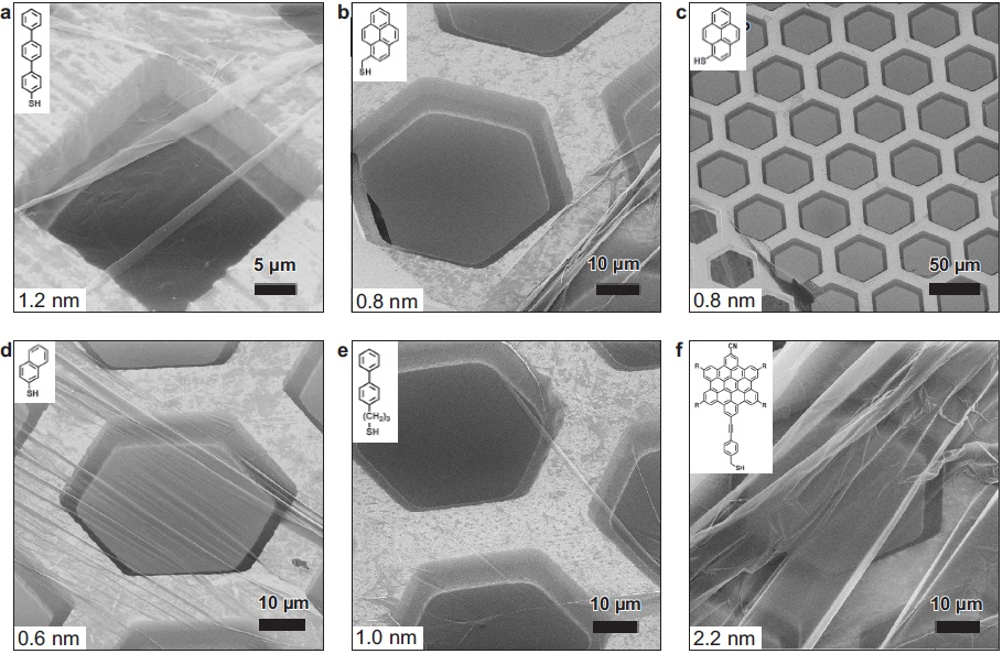
Figure 1: Macroscopic CNMs made from various precursors resting on support structures. Images, made using helium ion microscopy, are taken from [8] (with friendly permission).

Although the aromatic precursor molecules biphenyl, terphenyl and naphthalene thiols (BPT, TPT, NPTH, see Appendix B) are well-characterized, not much is known about the internal structure of such nanomembranes [17]. The reason is that existing characterization methods fail to deliver an accurate structure mainly due to the nanometer size thickness and the tiny weight, which, for example, does not allow accurate X-ray structure determination or infrared spectroscopy. In addition, the material is very likely highly disordered, which renders an X-ray structure determination nearly impossible.

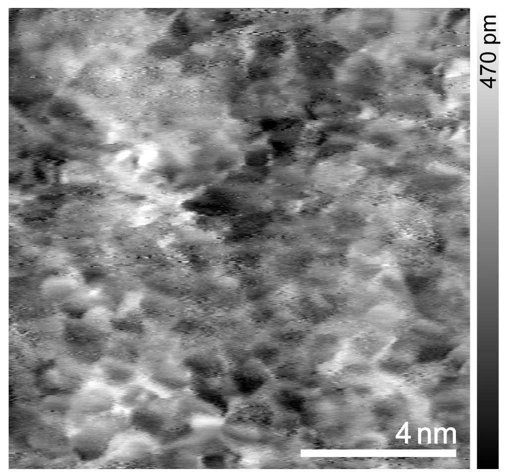
Figure 2: AFM tapping mode topography image of TPT CNM on Au, measured at 93 K in ultra-high vacuum (amplitude set point $A=7.6$ nm, center frequency $f_{0}=274.8$ kHz). The height information is black-to-white encoded, displaying the subnanoporous network of the nanomembrane.

On the other hand, the material can be produced to macroscopic dimensions, and it is mechanically stable, see Fig. 1. Therefore, macroscopic mechanical properties, such as Young’s moduli, can be determined for such membranes [18]. The moduli turn out to be of the order of $10$ GPa, i.e. the material is astonishingly soft compared to graphene ($1000$ GPa). It is also possible to study water permeation [19, 20] as well as electrical properties [21] in order to further characterize the membranes. Investigation by means of near edge X-ray absorption fine structure (NEXAFS) allows to estimate the aromaticity, i.e. the amount of intact aromatic carbon rings, as well as the $sp^{2}$ content still present in the CNM [22].

Atomic force microscopy (AFM) delivers topographic images of CNMs deposited on substrate material [20], compare Fig. 2. This allows to infer information of membrane structure on mesoscopic (nm) lateral scales, in particular the sizes and distribution of holes and voids across the membrane. The latter is closely related to transport properties of gases and liquids through the membrane [20].

In this article we report on first realistic and large-scale theoretical simulations of CNMs. Before we start, we would like to highlight the general problems that challenge such an investigation. This helps to understand why such simulations have not yet been done although CNMs already exist for about two decades.

1. Since quantum mechanical simulations are not at all feasible, we have to rely on a classical approach and thus unavoidably make an approximation. This holds in particular for the use of classical carbon-carbon interactions [23].

2. The CNM will be in a disordered metastable state, i.e. a local minimum in a huge configuration space. The true ground state of the material, which consists of pure carbon, would be a flake of graphite. It is very likely that a large number of disordered metastable states is actually equivalent in so far that they all constitute mechanically stable membranes. A crucial question is how much of the initial correlations imprinted in the precursor molecules survives and finally determines properties of the CNM.

3. How can we quantify whether a simulated structure is a realistic model of the true CNM? In view of the lack of structural information only indirect observables such as Young’s modulus, the topographic image, or the aromaticity may serve as guidance.

4. In addition, the imperfectness of the CNMs, i.e. the existence and distribution of holes, that leads to the fascinating property of water filtration [19, 20], can also serve as a clue. To this end larger CNMs have to be simulated in order to minimize finite-size and boundary effects.

For our simulations we employ classical molecular dynamics as implemented in the publicly available large atomic/molecular massively parallel simulator (LAMMPS) [24]. Our previous studies have shown that the potentials and algorithms implemented in LAMMPS are accurate to a large extent for other carbon-based systems as e.g. diamond, graphene, or nanotubes [23]. The environment-dependent interatomic potential (EDIP) of Marks [25, 26], not implemented in LAMMPS, appears superior in several contexts, and is thus also employed [27, 26, 3].

In order to incorporate at least the gross features of the production process we decided to mimic the formation of the CNM as a dynamical process that consists of excitation, compression as well as expansion and equilibration. This goes far beyond the more quasistatic approach of Ref. [17] used earlier.

We can summarize our findings as follows: It is indeed possible to simulate mechanically stable CNMs. We find production scenarios under which the membranes possess holes of the correct size as determined by AFM measurements [20]. We can also theoretically determine the Young’s modulus. It is systematically larger than experimentally found [18]. The reasons will be discussed later in the paper. We can also relate the number of perfect hexagons in the classical structures to the experimentally deduced aromaticity. It turns out that both, experiment and theory suggest, that stable CNMs contain a drastically reduced number of aromatic rings compared to their precursors. The broken-up rings seem to be a necessary prerequisite to deliver the “glue” for the stabilization of the membrane.

The article is organized as follows. In Sec. II we shortly repeat the essentials of classical molecular dynamics calculations as well as the technical details employed for the simulations. The main section III is devoted to the simulations of CNMs as well as to the determination of their physical properties. In the appendix we present first attempts to generate AFM images related to our simulations. The article closes with discussion and conclusions.

II Method and technical details

II.1 Classical carbon-carbon interaction

A realistic classical carbon-carbon interaction must be able to account for the various $sp^{n}$–binding modes. The program package LAMMPS offers several of such potentials, among them those developed by Tersoff and Brenner in various versions [28, 29, 30] as well as new extensions built on the original potentials.

In addition to the implemented potentials we are going to use the improved EDIP potential by Marks [25, 26] for some of our simulations, which so far is not included in standard versions of LAMMPS. Taking this potential as an example, we want to qualitatively explain how such potentials work. These potentials comprise density-dependent two- and three-body potentials, $U_{2}$ and $U_{3}$ in this example respectively,

$$U\left(\vec{R}_{1},\dots,\vec{R}_{N}\right) = \sum_{i=1}^{N}\Big{\{}\sum_{\begin{subarray}{c}j=1\\ j\neq i\end{subarray}}^{N}U_{2}(R_{ij},Z(i))$$

$$+ \sum_{\begin{subarray}{c}j=1\\ j\neq i\end{subarray}}^{N}\sum_{\begin{subarray}{c}k=j+1\\ k\neq i\end{subarray}}^{N}U_{3}(R_{ij},R_{ik},\theta(i,j,k),Z(i))\Big{\}}$$

which account for the various binding modes. This is achieved by an advanced parameterization in terms of a smooth coordination variable $Z(i)$ as well as by appropriate angle dependencies $\theta(i,j,k)$. The EDIP potential employs a cutoff of 3.2 Å and a dihedral penalty.

Another popular option for carbon-carbon (C-C) interactions is AIREBO [31], which also includes the necessary implementation for carbon-hydrogen (C-H) interactions. This potential is employed in our simulations when the virial per atom is needed, since this is not yet implemented for EDIP.

II.2 Modeling of the membrane

Modeling of a membrane is achieved through the following steps inspired by the experimental procedure as depicted in Fig. 3 and explained in detail in [8]. Our simulations include only carbon atoms, since the precursor molecules of the SAM lose practically all hydrogen atoms during electron irradiation, see experimental verification in [22, 9], such that the remaining carbon skeletons interlink to form the final CNM which thus is a form of pure carbon. All other atoms such as sulfur of the thiol are also neglected right from the beginning. The loss of carbon is small during the production process [8, 9], Table 1, but will nevertheless be addressed by us since it might have an impact on the formation of holes.

1. Formation of a self-assembled monolayer (SAM) from a selection of various precursor molecules on a gold substrate is initiated by placing carbon atoms above a gold surface at positions they would have in the respective precursor molecules (Initialization).

   Also, we replace the computationally expensive array of gold atoms representing the substrate by a repulsive Lennard-Jones wall potential

   $$V(r)=4\varepsilon\left[\left(\frac{\sigma}{r}\right)^{12}-\left(\frac{\sigma}{r}\right)^{6}\right],$$ (2)

   with its minimum $r_{min}=\sqrt[6]{2}\cdot\sigma$ at the bottom of the simulation box $z_{\text{lo}}$ and parameters for the C-Au interaction $\varepsilon_{C-Au}\approx 0.29256\leavevmode\nobreak\ \text{kcal/mol}\approx 0.012695$ eV and $\sigma_{C-Au}\approx 2.99$ Å taken from [32]. It should be mentioned however that this also leaves us with no structure of the substrate (except for the structural parameters of gold taken for the initial placement of the precursor molecules), which could have some influence on the formation process.

2. Then, specific starting conditions are imposed by tilting or randomly moving some or all molecules and by either removing some of the atoms or whole molecules to e.g. mimic defects in the experimental process (Randomization), see [27, 33, 26] and Table 1.

3. Experimentally, after low-energy electron irradiation of the SAM, crosslinking of the molecules induces the formation of the CNM. Theoretically, the electron irradiation is modeled by a vertical force gradient being applied to the atoms; it is linear and decreasing with height (Compression). It is assumed that secondary electrons actually cause most of the bond-breaking and crosslinking. The effect of secondary electrons is e.g. modeled by lateral forces on randomly selected molecules. In reality, processes probably follow a sequential order on a short time scale. This is neglected in the present simulations, in particular since it is not clear whether and how such correlations survive in the course of relaxation towards the final structure which happens on much longer time scales.

4. The model system is then allowed to relax towards an equilibrium structure according to a thermostat dynamics (Nosé-Hoover or Langevin) with a temperature that decreases linearly in time (Cooling). This corresponds to the fact that the gold support also acts as a very efficient heat sink during the synthesis process.

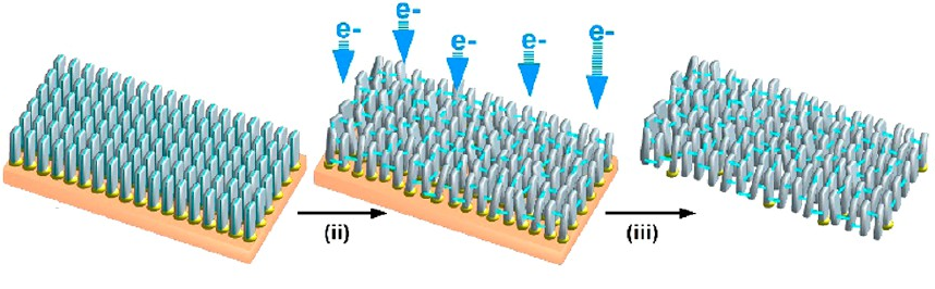
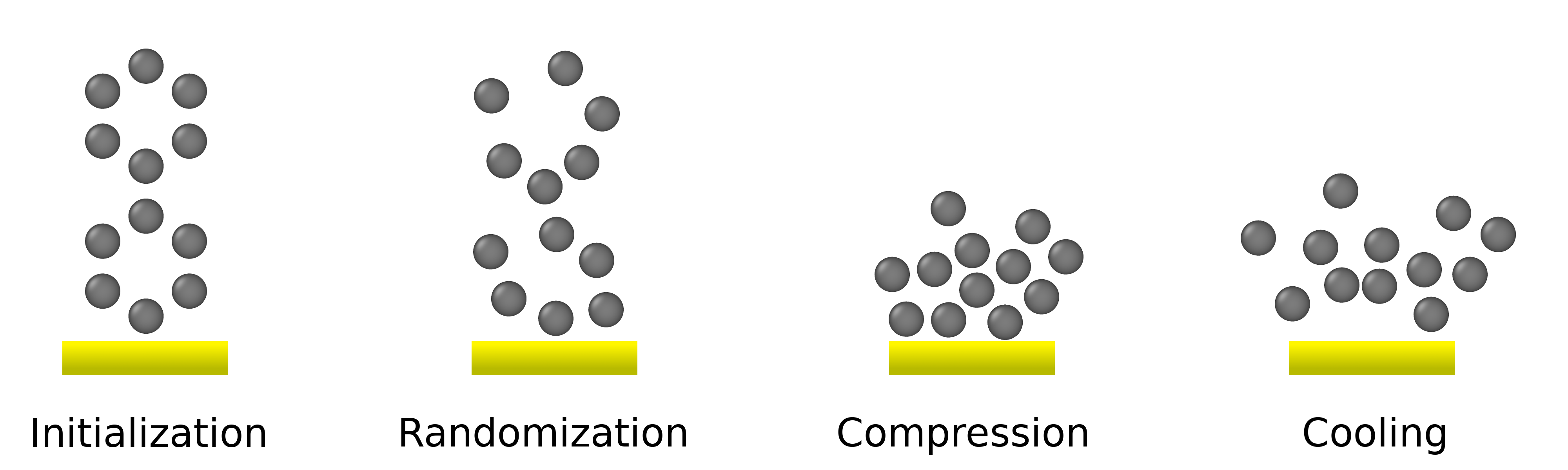
Figure 3: Top: Sketch of the experimental synthesis of a CNM, taken from  [8]. Bottom: Sketch of the theoretical four step synthesis model of a CNM starting from a precursor corresponding to BPT.

Measurements by X-ray photoelectron spectroscopy (XPS) presented in Table 1 provide a qualitative measure for the modeled membranes. The thickness of the membrane should remain close to the thickness of the original SAM, since there is only little loss of carbon during irradiation [8, 9].

Table 1: Experimental thickness and carbon loss as determined by XPS measurements [8].

	SAM thickness	CNM thickness	C loss
BPT	10Å	9Å	5 %
TPT	13Å	12Å	4 %
NPTH	6Å	6Å	9 %

We divide the outcomes of our simulation procedure into four categories depending on the parameters used: 1) weak randomization, i.e. there is only some randomization of atom coordinates, 2) randomization and compression, i.e. after randomization a vertical force is applied, 3) randomization, compression and lateral force that acts on some selected molecules, and 4) randomization, compression and randomly excluding molecules from the simulation.

II.3 Determination of the Young’s modulus

With the structures generated, we choose the Young’s modulus as our observable of choice as it allows comparison with experimental results (note that electronic properties cannot be covered by classical molecular dynamics). These calculations are realized in two ways:

1. We adapt LAMMPS’ own ELASTIC code as available in the example repository [34] to our needs which derives the Young’s modulus from the curvature of the potential Energy $U$. For this we use our own implementation of the EDIP.

2. We use a dynamical approach that stretches the membrane (stress vs. strain), thereby allowing for deformation and defect formation, and derives the modulus from the linear region of the stress-strain curve. Due to the lack of the virial per atom in our implementation of EDIP, we use the AIREBO potential for this type of simulation.

The Young’s modulus $E$ in the ground state, i.e. at temperature $T=0$ K, can be evaluated from the curvature of $U$ at the ground state configuration (the kinetic energy is zero) [35]

$$E_{V}=\frac{1}{V_{0}}\left(\frac{\partial^{2}U}{\partial\alpha^{2}}\right)_{\alpha=1}\ ,$$ (3)

where $\alpha$ is the factor by which all positions are scaled along the direction of the dimensionless unit vector $\vec{e}_{\alpha}$, i.e.

$$\vec{x}_{i}\rightarrow\vec{x}_{i}+(\alpha-1)\ \vec{e}_{\alpha}\cdot\vec{x}_{i}\ \vec{e}_{\alpha}\ .$$ (4)

$V_{0}$ denotes the cuboidic volume of the sample in equilibrium.

There is however a challenge when it comes to the definition of volume of a CNM due to its irregular internal structure. Thus one has to find ways to approximate the volume, which introduces inherent uncertainty into the results, since the variation of thickness is of the same order as the thickness itself. Possible approaches are presented in Sec. II.4.3.

Another approach is to derive the Young’s modulus from the relationship between stress $\sigma$ and strain $\varepsilon$ in the linear part of a stress-strain-curve as employed by materials science for macroscopic materials, i.e. by determining

$$E=\frac{\Delta\sigma}{\Delta\varepsilon}\ ,$$ (5)

which can be done in classical molecular dynamics by moving clamped parts of the material similar to experiments for material characterization. This is not directly transferable to real CNMs as they cannot be investigated this way due to their restricting size. The alternative way to experimentally characterize such thin membranes is by performing a bulge test [18] where the deflection of a membrane under pressure is measured by the tip of an atomic force microscope. This has been modeled as a molecular dynamics simulation for graphene in [36]. Here we do not use this method since there is no well defined profile of curvature of the membrane while for graphene there is even a formula for expressing the maximum height of the graphene sheet depending on the applied pressure difference. Also, one might have to resort to bigger molecules for the gas (for graphene hydrogen is used) when this model is transferred to CNMs as the holes possibly allow for gas molecules to pass through the membrane, making it hard to keep track of applied pressure when there is a vacuum on the other side.

II.4 Simulation setup

II.4.1 General setup

All simulations are done with shrink-wrapped boundary conditions (boundary s s s), which causes the simulation box to be non-periodic. We use metal units and a time step of $0.0001$. The primary pair_style, i.e. potential we employ is airebo in the current parameterization of LAMMPS stable release from 22. August 2018 in CH.airebo with a cutoff of $3.0$ as well as Lennard-Jones and torsion flags being set to $1$. For the EDIP we use our own implementation of Nigel Marks’ carbon-carbon potential [37] that is not available in the official LAMMPS repositories. We perform constant NVE integrations as implemented in LAMMPS, i.e. integrations with conctant particle number, constant volume, and constant energy.

II.4.2 Modeling process details

As for specific modeling setups we make use of velocity create to introduce randomization and fix addforce to apply downward momentum transfer to either all or some molecules or atoms. Selection of atoms and molecules is done by grouping the desired amount and preprocessing of the LAMMPS input script by external scripting means. The bottom wall representing the gold substrate is achieved by a repulsive Lennard-Jones potential as described above in (2) using wall/lj126. Wall potentials on the lateral sides of the membrane that prevent unwanted spreading are of the type wall/harmonic with a cutoff large enough to prevent atoms from passing the wall within a time step.

After the application of force or thermal randomization of atoms and molecules, the CNM is highly excited and has thus to be cooled. This is achieved by means of a Langevin-type thermostat as implemented in LAMMPS. The final structure of the membrane depends strongly on the parameters used for the thermostat, i.e. the damping rate of the Langevin thermostat has direct influence on how much time the atoms have to spread in the $z$-direction and thus making the membrane thicker and less dense. This has measurable influence on the Young’s modulus and is thus kept at the recommended best practice damping rate related to the time step, which in this case gives a damping of $0.001$. Other thermostats can be tweaked such that results are very similar to each other.

II.4.3 Postprocessing

Postprocessing takes care of adjusting the Young’s moduli with respect to the volume of the system. However, as this is not well-defined one has several options to calculate the volume. The first and simplest is to take the size of the simulation box, which does not account for voids. The second more involved method is to create a surface volume of the CNM that tries to minimize superficial empty volumes thus creating a shrinkwrap-like representation of the membrane’s volume. The latter and all of the visualization tasks are done with the software Ovito [38].

III Theoretical Investigations

III.1 Weak randomization

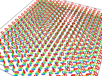
Figure 4: A typical result of minimization of a weakly randomized TPT-based CNM. Color represents position along $z$-direction (blue to red as on regular maps). The $x$-coordinate runs along the visible rows from bottom to top and the $y$-coordinate perpendicular to that, i.e. from left to right.

In this section we will discuss the results of the molecular dynamics simulations where only weak randomization is employed. As a reminder, randomization is one theoretical means to model the excitation of the SAM due to the electron bombardment. To this end, atoms of the SAM are given random displacements with respect to the initial configuration. The isotropic randomization corresponds to a temperature in the range $300-1100$ K. The system is then cooled down to find a stable configuration.

Resulting nanomembranes, as shown for TPT in Fig. 4, mostly retain the initial structure of the SAM. The excitation energies are not sufficient to break up carbon bonds and to create a disordered structure. This can be clearly seen in Fig. 4 where in addition the color code represents the height above the gold support. The membrane consists of weakly interacting upright terphenyls. Similar results have been obtained in the quasi static approach of Ref. [17]. Nevertheless, the membrane represents a bound state due to the attractive long range component of the carbon-carbon interaction, and it is mechanically stable. However, we consider such membranes unrealistic since they do not form any non-regularities such as holes observed by AFM and obviously needed for water permeation [20]. Membranes of all three investigated precursor molecules, BPT, TPT, and naphthalene, behave in the same way; we therefore show only a case of TPT.

The high density of the membrane is also reflected in the Young’s moduli presented in Table 2. Here and in the following, we show two values for each Young’s modulus to address the problem of volume in the definition of the Young’s modulus as previously discussed – the first adjusted to the volume of the simulation box and the second to the shrink-wrapped surface volume. Due to the very anisotropic structure of the simulated CNMs also the moduli are very anisotropic. The rather small Young’s modulus in the $y$-direction perpendicular to the rows for all precursor molecules can be explained by visual inspection of the carbon-carbon bonds existent in the membrane, compare Fig. 4. Due to the nature of the self-assembled monolayer, there is a larger distance between neighboring rows of molecules in the $y$-direction than there is between molecules in the $x$-direction. This is also the reason for stronger bonds forming in the $x$-direction.

Table 2: Young’s moduli in $x$- and $y$-direction adjusted to volume of simulation box$|$surface volume for single realizations of membranes. For direction of coordinates compare Fig. 4. Index 1 denotes method 1 (EDIP and curvature), index 2 denotes method 2 (AIREBO and stress).

	$E_{x,1}$/GPa	$E_{x,2}$/GPa	$E_{y,1}$/GPa	$E_{y,2}$/GPa
BPT	$266|576$	$33|71$	$139|301$	$66|143$
TPT	$373|398$	$52|56$	$40|43$	$287|309$
NPTH	$576|734$	$124|158$	$77|98$	$22|28$

III.2 Randomization and compression

III.2.1 Vertical momentum only

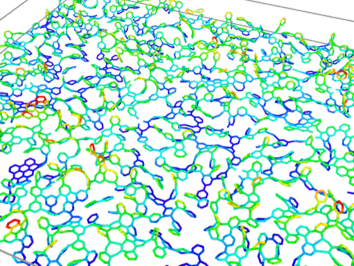
Figure 5: A typical result of vertical momentum dynamics applied to BPT-SAM, $T=700$ K, $k=60\leavevmode\nobreak\ \frac{\text{eV}}{\text{\AA}}$. Color represents position along $z$-direction (blue to red as on regular maps). $x$- and $y$-directions as in Fig. 4.

A more realistic approach is to apply a vertical momentum to the molecules of the self-assembled monolayer in direction of the gold substrate to simulate the momentum transfer of electrons to the atoms. Since most of the electrons’ energy should be absorbed at the top of molecules, we use a linear profile for the applied force using the LAMMPS command addforce, i.e. $F=-k\cdot(z-z_{\text{lo}})$, where $z_{\text{lo}}$ is the $z$-coordinate of the gold surface. During the time evolution of this procedure, atoms will be compressed towards and reflected away from the substrate. Time evolution is stopped when the height of the membrane approaches the initial monolayer height as experimentally observed membrane heights are close to the self-assembled monolayer [8]. Finally, the system is cooled using thermostat dynamics. We test multiple proportionality factors $k$ for the force profile ranging from $30\leavevmode\nobreak\ \frac{\text{eV}}{\text{\AA}}$ to $200\leavevmode\nobreak\ \frac{\text{eV}}{\text{\AA}}$ ($z$ and $z_{\text{lo}}$ being dimensionless), which is equivalent to a velocity range of $2.41\leavevmode\nobreak\ \frac{\text{\AA}}{\text{ps}}$ to $16.07\leavevmode\nobreak\ \frac{\text{\AA}}{\text{ps}}$. Additionally, the same randomization as in the previous section is applied to introduce some areas where bond formation might be preferred.

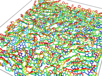
Figure 6: A typical result of vertical momentum dynamics applied to TPT-SAM, $T=700$ K, $k=30\leavevmode\nobreak\ \frac{\text{eV}}{\text{\AA}}$. Color represents position along $z$-direction (blue to red as on regular maps). $x$- and $y$-directions as in Fig. 4.

Visualizations of membranes created through this process can be seen in Fig. 5 to Fig. 7. We note that the resulting carbon networks are more irregular and contain remnants of broken aromatic rings that serve as linkers in the network. In particular, Fig. 5 shows a typical result for BPT. Since the precursor BPT consists of two phenyls only and a large fraction of these are broken up, the resulting membrane is rather flat (compare color code) and appears to consist of denser regions that are loosely connected by phenyl strings. Pentagonal structures, also reported in [39], are visible.

Figure 6 presents a simulation of a TPT-based nanomembrane. This membrane is thicker, since TPT consists of three phenyls. The structure appears to be more strongly connected in the $z$-direction (height). Voids and linear carbon strings are visible.

Naphthalene on the other hand is a rather small molecule, therefore the resulting CNM is rather flat and seems to contain deformed graphene-like parts, see Fig. 7. We speculate that the edge-sharing structure of the two rings in naphthalene, compare Table 9, is rather stable and promotes graphene-like patches.

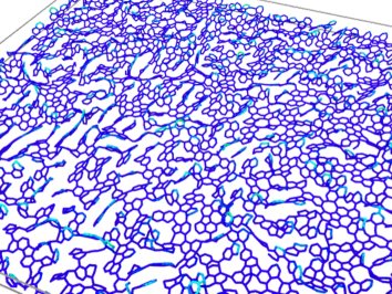
Figure 7: A typical result of vertical momentum dynamics applied to NPTH-SAM, $T=700$ K, $k=30\leavevmode\nobreak\ \frac{\text{eV}}{\text{\AA}}$. Color represents position along $z$-direction (blue to red as on regular maps). $x$- and $y$-directions as in Fig. 4.

The generated CNMs, which are mechanically stable, are characterized by rather large Young’s moduli, compare Tables 3 and 4. In particular, naphthalene precursors, that form rather flat and rigid membranes as discussed above exhibit moduli close to that of graphene. Both tables show a systematic dependence on the strength of the vertical force field characterized by $k$: The larger $k$, the smaller is the modulus. Due to larger effective randomization values along different directions are similar. Interestingly, there is a systematic difference in moduli between the two ways we compute them. Moduli calculated using the AIREBO potential and applying stress are systematically smaller compared to those using EDIP and the curvature of the potential energy. Reasons need to be investigated in the future.

Table 3: Method 1 (EDIP and curvature): Young’s moduli in $x$- and $y$-direction adjusted to volume of simulation box$|$surface volume for single realizations of membranes. For direction of coordinates compare Fig. 4.

	$E_{x,1}$/GPa	$E_{y,1}$/GPa
TPT (T=700 K, $k=30\leavevmode\nobreak\ \frac{\text{eV}}{\text{\AA}}$)	$436|847$	$334|649$
TPT (T=700 K, $k=200\leavevmode\nobreak\ \frac{\text{eV}}{\text{\AA}}$)	$215|448$	$220|457$
TPT (T=300 K, $k=60\leavevmode\nobreak\ \frac{\text{eV}}{\text{\AA}}$)	$325|987$	$316|960$
TPT (T=1100 K, $k=60\leavevmode\nobreak\ \frac{\text{eV}}{\text{\AA}}$)	$351|866$	$339|838$
BPT (T=700 K, $k=60\leavevmode\nobreak\ \frac{\text{eV}}{\text{\AA}}$)	$202|736$	$191|695$
NPTH (T=700 K, $k=60\leavevmode\nobreak\ \frac{\text{eV}}{\text{\AA}}$)	$536|1367$	$500|1277$

Table 4: Method 2 (AIREBO and stress): Young’s moduli in $x$- and $y$-direction adjusted to volume of simulation box$|$surface volume for single realizations of membranes. For direction of coordinates compare Fig. 4.

	$E_{x,2}$/GPa	$E_{y,2}$/GPa
TPT (T=700 K, $k=30\leavevmode\nobreak\ \frac{\text{eV}}{\text{\AA}}$)	$135|262$	$77|150$
TPT (T=700 K, $k=200\leavevmode\nobreak\ \frac{\text{eV}}{\text{\AA}}$)	$45|92$	$40|83$
TPT (T=300 K, $k=60\leavevmode\nobreak\ \frac{\text{eV}}{\text{\AA}}$)	$122|371$	$97|295$
TPT (T=1100 K, $k=60\leavevmode\nobreak\ \frac{\text{eV}}{\text{\AA}}$)	$123|303$	$100|247$
BPT (T=700 K, $k=60\leavevmode\nobreak\ \frac{\text{eV}}{\text{\AA}}$)	$16|58$	$19|69$
NPTH (T=700 K, $k=60\leavevmode\nobreak\ \frac{\text{eV}}{\text{\AA}}$)	$99|252$	$45|115$

III.3 Additional lateral momentum

In order to mimic the influence of secondary electrons and their interaction with neighboring molecules and atoms, we incorporate additional lateral momenta of various magnitude as shown in Tables 5 and 6. We apply an isotropic but randomly chosen lateral force to all atoms using the same LAMMPS fix addforce as before. Tables 5 and 6 show averages over 10 realizations of such membranes depending on the theoretical synthesis procedure. By applying lateral momenta there is a higher chance for holes to form due to displacement in the $x$- and $y$-directions. This also affects membrane thickness and surface roughness. This method relies highly on the randomly chosen lateral force by which molecules are laterally displaced. Realistically, forces would not be isotropic throughout the membrane. Thus the Young’s modulus is averaged over ten different configurations each. Again, the values of method 2 are systematically smaller compared to method 1 and also closer to the experimentally determined moduli.

Table 5: Method 1 (EDIP and curvature): Young’s moduli in $x$-direction adjusted to volume of simulation box$|$surface volume. Numbers in parenthesis provide standard deviations for the averages taken over 10 realizations.

$v$ / $\frac{\text{\AA}}{\text{ps}}$	TPT: $E_{x,1}$/GPa	BPT: $E_{x,1}$/GPa	NPTH: $E_{x,1}$/GPa
$5$	$338(55)|925(18)$	$246(14)|782(12)$	$588(41)|2002(47)$
$15$	$299(20)|858(24)$	$195(25)|888(15)$	$546(32)|1865(38)$
$25$	$224(46)|769(20)$	$166(16)|818(24)$	$497(25)|1579(49)$
$35$	$268(46)|738(32)$	$139(12)|732(12)$	$410(34)|1393(40)$

Table 6: Method 2 (AIREBO and stress): Young’s moduli in $x$-direction adjusted to volume of simulation box$|$surface volume. Numbers in parenthesis provide standard deviations for the averages taken over 10 realizations.

$v$ / $\frac{\text{\AA}}{\text{ps}}$	TPT: $E_{x,2}$/GPa	BPT: $E_{x,2}$/GPa	NPTH: $E_{x,2}$/GPa
$5$	$120(23)|328(63)$	$25(4)|79(13)$	$201(32)|684(109)$
$15$	$98(12)|281(34)$	$23(5)|105(23)$	$144(28)|492(96)$
$25$	$62(14)|213(48)$	$19(4)|94(20)$	$114(34)|362(108)$
$35$	$68(11)|187(30)$	$16(3)|84(16)$	$95(23)|323(78)$

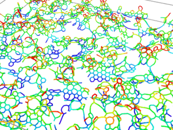
Figure 8: A typical result of vertical and lateral momentum dynamics applied to BPT-SAM after 4900 time steps, $T=300$ K, $v=35\leavevmode\nobreak\ \frac{\text{\AA}}{\text{ps}}$, $k=60\leavevmode\nobreak\ \frac{\text{eV}}{\text{\AA}}$. Color represents position along $z$-direction (blue to red as on regular maps). $x$- and $y$-directions as in Fig. 4.

One can clearly see large holes for the biphenyl-based and naphthalene-based CNMs in Figs. 8 and 9, respectively. Both structures appear to be bunched, i.e. they possess denser areas that are connected by strings of carbon atoms or of phenyl rings. For the realization of a terphenyl-based membrane depicted in Fig. 10, holes appear not as pronounced, but there is increased roughness compared to the previous results, i.e. more pronounced valleys and hills in both height and lateral distance from each other. Nevertheless, also TPT nanomembranes exhibit an increased number of holes.

These qualitative results are also reflected in the quantitative results for the Young’s modulus, see Tables 5 and 6. With increasing magnitude of the lateral force there is a decrease in the Young’s modulus for all precursor molecules. Only for the largest $v=35\frac{\text{\AA}}{\text{ps}}$ the terphenyl-based nanomembrane’s Young’s modulus increases, which might be related to the height of the precursor molecule. While biphenyl and naphthalene are basically two carbon rings tall, terphenyl is about $50$ % higher. This gives rise to the possibility of bonds to form on top of the membrane allowing increased surface roughness and more dense linking thereby increasing the Young’s modulus.

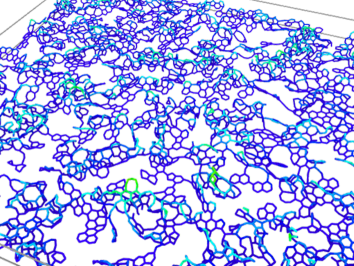
Figure 9: A typical result of vertical and lateral momentum dynamics applied to NPTH-SAM after 2500 time steps, $T=300$ K, $v=35\leavevmode\nobreak\ \frac{\text{\AA}}{\text{ps}}$, $k=60\leavevmode\nobreak\ \frac{\text{eV}}{\text{\AA}}$. Color represents position along $z$-direction (blue to red as on regular maps). $x$- and $y$-directions as in Fig. 4.

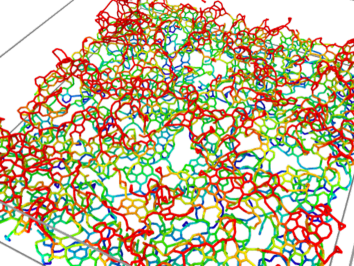
Figure 10: A typical result of vertical and lateral momentum dynamics applied to TPT-SAM after 5700 time steps, $T=700$ K, $v=35\leavevmode\nobreak\ \frac{\text{\AA}}{\text{ps}}$, $k=30\leavevmode\nobreak\ \frac{\text{eV}}{\text{\AA}}$. Color represents position along $z$-direction (blue to red as on regular maps). $x$- and $y$-directions as in Fig. 4.

III.4 Randomly missing molecules

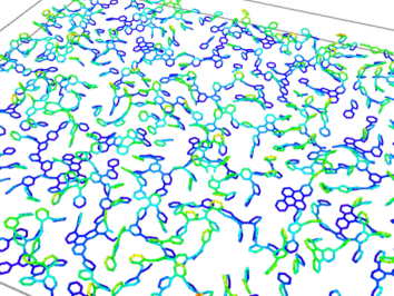
Figure 11: A typical result of vertical momentum dynamics with missing molecules applied to BPT-SAM after 4900 time steps, $T=300$ K, $k=60\leavevmode\nobreak\ \frac{\text{eV}}{\text{\AA}}$. Color represents position along $z$-direction (blue to red as on regular maps). $x$- and $y$-directions as in Fig. 4.

By randomly removing molecules from the self-assembled monolayer one can enhance the formation of holes in the resulting membrane. It is experimentally verified that about 5 to 9 % of carbon atoms get lost during synthesis [8]. Our process models a correlated/collective disappearance of atoms in form of whole molecules. We consider percentages of removal ranging from $5$ to $20$ %. Areas where molecules are missing are preferred locations of holes as applied vertical momentum can only cover the gaps to a limited degree. This also gives rise to the possibility of further lowering the Young’s modulus. The resulting CNMs show a less dense structure than before. Holes have the tendency to be smaller but more frequent due to the more isotropic distribution of missing molecules, which can be seen in Figs. 11, 12, and 13.

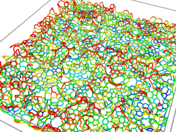
Figure 12: A typical result of vertical momentum dynamics with missing molecules applied to TPT-SAM after 7200 time steps, $T=300$ K, $k=60\leavevmode\nobreak\ \frac{\text{eV}}{\text{\AA}}$. Color represents position along $z$-direction (blue to red as on regular maps). $x$- and $y$-directions as in Fig. 4.

Again, BPT- and NPT-based membranes, Figs. 11, and 13 turn out to be rather thin with graphene-like patches. This seems to be a common and rather stable motif under many conditions of preparation. The chosen example of a TPT-based nanomembrane, Fig. 12 appears rather dense, even denser than the sample shown in Fig. 10 that had not experienced any random losses of precursor molecules. This might be a coincidence and therefore calls for future large scale simulations to generate sufficient statistics.

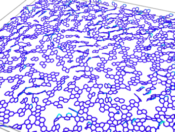
Figure 13: A typical result of vertical momentum dynamics with missing molecules applied to NPTH-SAM after 2500 time steps, $T=300$ K, $k=60\leavevmode\nobreak\ \frac{\text{eV}}{\text{\AA}}$. Color represents position along $z$-direction (blue to red as on regular maps). $x$- and $y$-directions as in Fig. 4.

When it comes to quantitative results, the differences in Young’s moduli are not as pronounced as the visual differences, compare Tables 7 and 8. The moduli decrease by $10$ to $20$ % at most. Even if there is significant carbon loss when irradiating the SAM, the newly created bonds are too isotropic to allow for softer areas. Thus any local weak spot is corrected by molecules arranging flatter than before. This is best observed for the naphthalene-based carbon nanomembrane shown in Fig. 13, where one can see large areas of intact hexagonal carbon rings strengthening the overall membrane and yielding a larger modulus.

Table 7: Method 1: Young’s moduli in $x$-direction for different deletion percentages adjusted to volume of simulation box$|$surface volume.

$p$ / %	TPT: $E_{x,1}$/GPa	BPT: $E_{x,1}$/GPa	NPTH: $E_{x,1}$/GPa
$5$	$368|1011$	$220|704$	$620|2313$
$10$	$255|976$	$177|787$	$579|1689$
$20$	$329|1000$	$193|824$	$558|2437$

Table 8: Method 2: Young’s moduli in $x$-direction for different deletion percentages adjusted to volume of simulation box$|$surface volume.

$p$ / %	TPT: $E_{x,2}$/GPa	BPT: $E_{x,2}$/GPa	NPTH: $E_{x,2}$/GPa
$5$	$131|360$	$21|67$	$135|503$
$10$	$86|329$	$16|71$	$50|146$
$20$	$105|319$	$16|68$	$40|175$

IV Discussion and Conclusions

Our goal was to create first computer simulations that model the process of CNM formation as realistically as possible. In order to achieve this goal we suggest various scenarios abstracting the experimental process such that the formation can be modeled by classical molecular dynamics.

We have shown that some processes deliver membranes that appear closer to the experiment than others. The most violent approaches, applying both vertical and lateral momentum transfer, are able to produce better results with respect to the visual impression of the membrane in particular concerning holes needed for its filtration abilities. This is a crucial step in understanding the internal structure of the membrane and possible molecular and atomic processes involved.

Results fall shorter when it comes to reproducing the experimental value of the Young’s modulus, which experimentally can be determined by various means, e.g. bulge tests, to be at least an order of magnitude smaller than our results. This is where the layers of abstraction play a big role. There are no hydrogen atoms and electrons present in our model system. Thus, breaking carbon-hydrogen bonds and momentum transfer by hydrogen atoms is only effectively included. Missing electron dynamics may strongly simplify the intricate momentum transfer, e.g. by secondary electrons.

However, all abstractions have to be made in order to be able to simulate large enough systems of carbon atoms and thus a reasonably sized area of a membrane. Other more accurate simulations, e.g. done by density functional theory (DFT) are limited to rather small numbers of atoms of order $10^{2}$ [40] or have to introduce periodicity into the simulation [39], which is a clear bias.

We are nevertheless confident that further progress will be possible. For example, in future investigations selected membranes will be simulated that contain a certain amount of hydrogen. This requires the use of classical carbon-hydrogen potentials such as for instance AIREBO. On the experimental side, it is planned to do ion scattering in order to determine structural correlations of CNMs [41, 42, 43].

A problem inherent to all simulations of atomic processes consists in the large span of time scales. The intrinsic time step is of order picosecond whereas some processes might need milliseconds. This means that one usually cannot model the relatively slow relaxation into the final state. Here workarounds have been developed recently [44] that artificially speed up such processes by an appropriately chosen higher temperature. It will also be investigated whether such a treatment would modify the theoretical formation process.

In a future investigation we are going to start a mass production of simulations for better statistics, in particular hole distributions as well as size distributions in dependence of production conditions. This is also needed for the idea to compare experimental AFM images with surfaces of simulated membranes. We would like to show first attempts along these lines in the appendix.

Appendix A Stylized model (artist’s view) of atomic force microscopy

One approach to create a visual impression of a nanomembrane is to employ atomic force microscopy (AFM) as e.g. done in [19]. The basic procedure is to rasterize the membrane using a cantilever and by that render atomic structures as well as valleys and holes visible. However, due to limited resolution of this approach, there is no certainty as to whether there are real holes or channels in the membrane. As demonstrated above, the visualization of molecular dynamics simulations is perfect in the sense that it shows the actual position of atoms and bonds. It is thus hard to compare these results to experimental atomic force microscopy images.

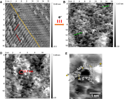
Figure 14: Experimental scanning probe and atomic force microscopy images of a TPT-based CNM [19] (with friendly permissions). See also Ref. [45].

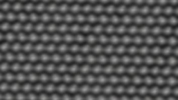
Figure 15: Simulated atomic force microscopy image of a TPT-based self-assembled monolayer.

Figure 16: Two versions of a simulated atomic force microscopy image of the TPT-based CNM shown in Fig. 10. The chosen theoretical color code determines the impression of depth strongly.

Here we present a stylized and artistic approach to generate images that have the same color scheme, i.e. representation of height, as atomic force microscopy and have (artificially) limited resolution as to which smallest structures can be resolved. It should be noted that this is by no means a quantitative measure as it is highly dependent on degrees of freedom of visualization parameters. The images have been created using the open-source software Blender [46].

An experimental result of atomic force microscopy of a TPT-based membrane taken from Ref. [19] is shown in Fig. 14. Panel A shows the SAM, panel B the crosslinked CNM; D and E display a possible hole and a hypothetical arrangement of TPT around the hole. For comparison, Fig. 15 shows the initial self assembled monolayer of terphenyls as used in our simulations, and Fig. 16 displays a resulting membrane, respectively. The parameters for this membrane are $T=700$ K, $v=35\leavevmode\nobreak\ \frac{\text{\AA}}{\text{ps}}$ and $k=30\leavevmode\nobreak\ \frac{\text{eV}}{\text{\AA}}$; the membrane is the same as in Fig. 10. Figure 16 also demonstrates that the chosen theoretical color code determines the impression of depth rather strongly. Nevertheless, this might be of great help in interpreting similar experimental pictures in order to unambiguously identify holes.

Appendix B Investigated precursor SAMs

Table 9: Precursor molecules and structures of the respective self assembled monolayers.

Name	Structural formula	SAM structure
Biphenyl-4-thiol (BPT) 1,1’-Biphenyl-4-thiol 4-Biphenylylthiol 4-Mercaptobiphenyl 4-Phenylbenzenethiol	[47]	(2 x 2) hexagonal, $\gamma=30^{\circ}$ [48] $\gamma=15^{\circ}$ [1] $\gamma=20^{\circ}$ [49] $\gamma=20^{\circ}$ [50]
		mixture of: (2 x 2) structure, (2$\sqrt{3}$ x 9) unit cell, (2$\sqrt{3}$ x 8) unit cell [48]
1,1’,4’,1”-Terphenyl-4-thiol (TPT)	[51]	$(\sqrt{3}$ x $\sqrt{3})$ structure $(2\sqrt{3}$ x $\sqrt{3})$ unit cell $\gamma=20^{\circ}$ [49]
2-Naphthalenethiol (NPTH) 2-Naphthyl mercaptan Thio-2-naphthol ($\beta$)	[52]	$(\sqrt{3}$ x $\sqrt{3})$ structure $(2\sqrt{3}$ x $\sqrt{3})$ unit cell

References

- Geyer et al. [1999] W. Geyer, V. Stadler, W. Eck, M. Zharnikov, A. Gölzhäuser, and M. Grunze, Appl. Phys. Lett. 75, 2401 (1999).
- Turchanin [2017] A. Turchanin, Annalen der Physik 529, 1700168 (2017), 1700168.
- de Tomas et al. [2019] C. de Tomas, A. Aghajamali, J. L. Jones, D. J. Lim, M. J. Lopez, I. Suarez-Martinez, and N. A. Marks, Carbon 155, 624 (2019).
- Dementyev et al. [2019] P. Dementyev, T. Wilke, D. Naberezhnyi, D. Emmrich, and A. Gölzhäuser, Phys. Chem. Chem. Phys. 21, 15471 (2019).
- Winter et al. [2019] A. Winter, Y. Ekinci, A. Gölzhäuser, and A. Turchanin, 2D Materials 6, 021002 (2019).
- Jakšić and Jakšić [2020] Z. Jakšić and O. Jakšić, Biomimetics 5, 24 (2020).
- Turchanin et al. [2009a] A. Turchanin, A. Beyer, C. T. Nottbohm, X. Zhang, R. Stosch, A. Sologubenko, J. Mayer, P. Hinze, T. Weimann, and A. Gölzhäuser, Adv. Mater. 21, 1233 (2009a).
- Angelova et al. [2013] P. Angelova, H. Vieker, N.-E. Weber, D. Matei, O. Reimer, I. Meier, S. Kurasch, J. Biskupek, D. Lorbach, K. Wunderlich, L. Chen, A. Terfort, M. Klapper, K. Müllen, U. Kaiser, A. Gölzhäuser, and A. Turchanin, ACS Nano 7, 6489 (2013).
- Turchanin and Gölzhäuser [2016] A. Turchanin and A. Gölzhäuser, Adv. Mater. 28, 6075 (2016).
- Matei et al. [2013] D. G. Matei, N.-E. Weber, S. Kurasch, S. Wundrack, M. Woszczyna, M. Grothe, T. Weimann, F. Ahlers, R. Stosch, U. Kaiser, and A. Turchanin, Adv. Mater. 25, 4146 (2013).
- Rhinow et al. [2012] D. Rhinow, N.-E. Weber, and A. Turchanin, J. Phys. Chem. C 116, 12295 (2012).
- Zhang et al. [2014] X. Zhang, C. Neumann, P. Angelova, A. Beyer, and A. Gölzhäuser, Langmuir 30, 8221 (2014), https://doi.org/10.1021/la501961d .
- Waske et al. [2012] P. A. Waske, N. Meyerbröker, W. Eck, and M. Zharnikov, J. Phys. Chem. C 116, 13559 (2012), http://pubs.acs.org/doi/pdf/10.1021/jp210768y .
- Love et al. [2005] J. C. Love, L. A. Estroff, J. K. Kriebel, R. G. Nuzzo, and G. M. Whitesides, Chem. Rev. 105, 1103 (2005).
- Schmid et al. [2019] M. Schmid, X. Wan, A. Asyuda, and M. Zharnikov, J. Phys. Chem. C 123, 28301 (2019).
- [16] A. Gölzhäuser, Private communication.
- Mrugalla and Schnack [2014] A. Mrugalla and J. Schnack, Beilstein J. Nanotechnol. 5, 865 (2014).
- Zhang et al. [2011] X. Zhang, A. Beyer, and A. Gölzhäuser, Beilstein J. Nanotechnol. 2, 826 (2011).
- Yang et al. [2018] Y. Yang, P. Dementyev, N. Biere, D. Emmrich, P. Stohmann, R. Korzetz, X. Zhang, A. Beyer, S. Koch, D. Anselmetti, et al., ACS nano 12, 4695 (2018).
- Yang et al. [2020] Y. Yang, R. Hillmann, Y. Qi, R. Korzetz, N. Biere, D. Emmrich, M. Westphal, B. Büker, A. Hütten, A. Beyer, D. Anselmetti, and A. Gölzhäuser, Advanced Materials 32, 1907850 (2020).
- Zhang et al. [2018] X. Zhang, E. Marschewski, P. Penner, T. Weimann, P. Hinze, A. Beyer, and A. Gölzhäuser, ACS nano 12, 10301 (2018).
- Turchanin et al. [2009b] A. Turchanin, D. Käfer, M. El-Desawy, C. Wöll, G. Witte, and A. Gölzhäuser, Langmuir 25, 7342 (2009b).
- Gayk et al. [2018] F. Gayk, J. Ehrens, T. Heitmann, P. Vorndamme, A. Mrugalla, and J. Schnack, Physica E 99, 215 (2018).
- Plimpton [1995] S. Plimpton, J. Comp. Phys. 117, 1 (1995), http://lammps.sandia.gov.
- Marks [2000] N. A. Marks, Phys. Rev. B 63, 035401 (2000).
- Martin et al. [2019] J. W. Martin, C. de Tomas, I. Suarez-Martinez, M. Kraft, and N. A. Marks, Phys. Rev. Lett. 123, 116105 (2019).
- de Tomas et al. [2016] C. de Tomas, I. Suarez-Martinez, and N. A. Marks, Carbon 109, 681 (2016).
- Tersoff [1988] J. Tersoff, Phys. Rev. B 37, 6991 (1988).
- Brenner [1990] D. W. Brenner, Phys. Rev. B 42, 9458 (1990).
- Brenner et al. [2002] D. W. Brenner, O. A. Shenderova, J. A. Harrison, S. J. Stuart, B. Ni, and S. B. Sinnott, J. Phys.: Cond. Mat. 14, 783 (2002).
- Stuart et al. [2000] S. J. Stuart, A. B. Tutein, and J. A. Harrison, J. Chem. Phys. 112, 6472 (2000).
- Khusenov et al. [2016] M. Khusenov, E. Dushanov, K. Kholmurodov, M. Zaki, and N. Sweilam, The Open Biochemistry Journal 10, 17 (2016).
- Shiell et al. [2018] T. B. Shiell, D. G. McCulloch, D. R. McKenzie, M. R. Field, B. Haberl, R. Boehler, B. A. Cook, C. de Tomas, I. Suarez-Martinez, N. A. Marks, and J. E. Bradby, Phys. Rev. Lett. 120, 215701 (2018).
- Corporation [2019] S. Corporation, Example scripts (2019), [Online; accessed 12-August-2019].
- Hernández et al. [1998] E. Hernández, C. Goze, P. Bernier, and A. Rubio, Phys. Rev. Lett. 80, 4502 (1998).
- Jun et al. [2011] S. Jun, T. Tashi, and H. S. Park, Journal of Nanomaterials 2011 (2011).
- Gayk [2018] F. Gayk, Simulation von Kohlenstoff-Nanomembranen mittels klassischer Molekulardynamik unter Verwendung des “environment-dependent interaction potential”, Master’s thesis, Bielefeld University (2018).
- Stukowski [2010] A. Stukowski, Modelling Simul. Mater. Sci. Eng. 18, 015012 (2010).
- Cabrera-Sanfelix et al. [2010] P. Cabrera-Sanfelix, A. Arnau, and D. Sanchez-Portal, Phys. Chem. Chem. Phys. 12, 1578 (2010).
- Marks et al. [2002] N. A. Marks, N. C. Cooper, D. R. McKenzie, D. G. McCulloch, P. Bath, and S. P. Russo, Phys. Rev. B 65, 075411 (2002).
- Wilhelm and Grande [2019] R. A. Wilhelm and P. L. Grande, Commun. Phys. 2, 89 (2019).
- Wilhelm [2020] R. A. Wilhelm, J. Phys.: Conf. Ser. 1412, 062010 (2020).
- [43] R. Wilhelm, Private communication.
- de Tomas et al. [2017] C. de Tomas, I. Suarez-Martinez, F. Vallejos-Burgos, M. J. Lopez, K. Kaneko, and N. A. Marks, Carbon 119, 1 (2017).
- Biere et al. [2019] N. Biere, S. Koch, P. Stohmann, V. Walhorn, A. Gölzhäuser, and D. Anselmetti, J. Phys. Chem. C 123, 19659 (2019).
- Community [2020] B. O. Community, Blender - a 3D modelling and rendering package, Blender Foundation, Amsterdam (2020).
- Sigma-Aldrich [2020a] Sigma-Aldrich, Biphenyl-4-thiol (2020a), [Online; accessed 28-August-2018].
- Matei et al. [2012] D. G. Matei, H. Muzik, A. Gölzhäuser, and A. Turchanin, Langmuir 28, 13905 (2012).
- Frey et al. [2001] S. Frey, V. Stadler, K. Heister, W. Eck, M. Zharnikov, M. Grunze, B. Zeysing, and A. Terfort, Langmuir 17, 2408 (2001).
- Heimel et al. [2008] G. Heimel, L. Romaner, J.-L. Brédas, and E. Zojer, Langmuir 24, 474 (2008).
- Sigma-Aldrich [2020b] Sigma-Aldrich, 1,1’,4’,1”-terphenyl-4-thiol (2020b), [Online; accessed 28-August-2018].
- Sigma-Aldrich [2020c] Sigma-Aldrich, 2-naphthalenethiol (2020c), [Online; accessed 28-August-2018].