Photospheric Velocity Gradients and Ejecta Masses of Hydrogen-poor Superluminous Supernovae – Proxies for Distinguishing between Fast and Slow Events

Abstract

We present a study of 28 Type I superluminous supernovae (SLSNe) in the context of the ejecta mass and photospheric velocity. We combine photometry and spectroscopy to infer ejecta masses via the formalism of radiation diffusion equations. We show an improved method to determine the photospheric velocity by combining spectrum modeling and cross correlation techniques. We find that Type I SLSNe can be divided into two groups by their pre-maximum spectra. Members of the first group have the W-shaped absorption trough in their pre-maximum spectrum, usually identified as due to O II. This feature is absent in the spectra of supernovae in the second group, whose spectra are similar to SN 2015bn. We confirm that the pre- or near-maximum photospheric velocities correlate with the velocity gradients: faster evolving SLSNe have larger photosheric velocities around maximum. We classify the studied SLSNe into the Fast or the Slow evolving group by their estimated photosheric velocities, and find that all those objects that resemble to SN 2015bn belong to the Slow evolving class, while SLSNe showing the W-like absorption are represented in both Fast and Slow evolving groups. We estimate the ejecta masses of all objects in our sample, and obtain values in the range of 2.9 ($\pm$0.8) - 208 ($\pm$61) $M_{\odot}$, with a mean of $43(\pm 12)~{}M_{\odot}$. We conclude that Slow evolving SLSNe tend to have higher ejecta masses compared to the Fast ones. Our ejecta mass calculations suggests that SLSNe are caused by energetic explosions of very massive stars, irrespectively of the powering mechanism of the light curve.

1 Introduction

A new class of transients, the so-called superluminous supernovae (SLSNe), was discovered and extensively studied in the past two decades. These extremely luminous events have at least ${\sim}10^{51}\,{\rm erg}$ total radiated energy, leading to an absolute brightness of $M<-21$ in all bands of the optical wavelengths (Gal-Yam, 2012, 2019). It has also been reported that these supernovae (SNe) prefer to explode in dwarf galaxies having low metallicity and high specific star-formation rate (Lunnan et al., 2013, 2014; Leloudas et al., 2015; Angus et al., 2016; Japelj et al., 2016; Perley et al., 2016; Schulze et al., 2018; Hatsukade et al., 2018), although some counterexamples are also known. For example, PTF10tpz (Arabsalmani et al., 2019), PTF10uhf (Perley et al., 2016) and SN 2017egm (Chen et al., 2017; Bose et al., 2018; Izzo et al., 2018; Yan et al., 2018; Hatsukade et al., 2020) occured in relatively bright and metal-rich, or, at least not metal-poor, host galaxies. The recent publications of De Cia et al. (2018); Lunnan et al. (2018), and Angus et al. (2019) revealed that this population is quite multitudinous: some lower luminosity transients (e.q. DES14C1rhg with $M_{r}=-19.4$; Angus et al. 2019) have also been classified as superluminous supernovae, because of the similar photometric or spectroscopic evolution to known, well-observed SLSNe (e.g. Quimby et al., 2018).

Similarly to the traditional/normal supernovae, SLSNe can also be separated into two main sub-classes: the H-poor Type I, and the H-rich Type II SLSN group (Branch & Wheeler, 2017). SLSNe-II are divided into two distinct populations: the luminosity of Type IIn SLSNe is powered by the strong interaction with the surrounding, massive circumstellar medium (CSM, e.q. SN 2006gy; Smith et al. 2007 or CSS121015; Benetti et al. 2014), and have similar spectroscopic properties and evolution to normal Type IIn SNe (Branch & Wheeler, 2017). The representatives of the second group, called normal Type II SLSNe show no visible signs of the CSM-interaction (e.g. SN 2013hx and PS15br; Inserra et al. 2018).

This study focuses on several events belonging to the H-poor SLSN-class. The members of SLSNe-I are usually revealed to be spectroscopically similar to normal Ic or BL-Ic SNe (e.g. Pastorello et al., 2010; Yan et al., 2015, 2017), with the difference that events in the former class have larger luminosities. SLSNe-I can be also separated into two groups (Inserra et al., 2018): the Fast (e.g. SN 2005ap; Lunnan et al. 2013) and the Slow evolving events (e.g. SN 2010kd; Kumar et al. 2020; Könyves-Tóth et al. 2020), with an average light curve (LC) rise-time of $\sim 28$ days, and $\sim 52$ days, respectively. Inserra et al. (2018) examined a sample of SLSNe statistically, and showed that Slow evolving SLSNe exhibit lower, and slowly evolving, or nearly constant photospheric velocities ($v\lesssim 12000$ km s^-1) from the maximum to +30 days phase, compared to the Fast evolving events having $v\gtrsim 12000$ km s^-1, and larger velocity gradients. However, some studies suggest that the transition between Fast and Slow events is continuous: e.g. Gaia16apd (SN 2016eay) was found to be a SLSN with LC time-scale in between those of the two groups (Kangas et al., 2017).

In many cases the pre-maximum, photospheric phase spectra of Type I SLSNe can be distinguished from lower luminosity Type Ic and BL-Ic events by a peculiar W-like absorption blend between 3900 and 4500 Å, which is identified to be due to O II (e.g. Liu et al., 2017). Alternatively, this feature can be modeled using the mixture of different ions, e.g. O III and C III (Quimby et al., 2007; Dessart, 2019; Gal-Yam, 2019b; Könyves-Tóth et al., 2020).

In this paper, we present ejecta mass calculations for a sample of 28 Type I SLSNe, using publicly available photometric and spectroscopic data. Our sample selection process is described in Section 3.

Recently, a similar study of SLSNe was carried out by Nicholl et al. (2015) who inferred the ejecta mass ($M_{\rm ej}$) of 24 SLSNe-I from bolometric LC modeling using the magnetar powering mechanism of the LC (Maeda et al., 2007), resulting in an average $M_{\rm ej}$ of 10 $M_{\odot}$, with a range of 3 and 30 $M_{\odot}$ for their sample. Yu et al. (2017) also inferred the ejecta mass of 31 SLSNe by fitting their bolometric LCs utilizing the magnetar engine model. On the other hand, from pair instability supernova (PISN; e.g. Gal-Yam 2009; Kasen et al. 2011) models, Lunnan et al. (2018) showed that the ejecta mass of some SLSNe may exceed far the values inferred by Nicholl et al. (2015) from the magnetar model: for example, the initial mass of iPTF16eh was estimated to be 115 $M_{\odot}$.

In our study the ejecta masses were inferred directly from the formulae derived by Arnett (1980) (shown in detail in Section 2), instead of full bolometric LC modeling. Our approach has the advantage of being independent from the assumed powering mechanism as long as the heating source is centrally located and the ejecta is optically thick, which are probably valid assumptions during the pre-maximum phases.

In our calculations the photospheric velocities ($v_{\rm phot}$) of the examined SLSNe measured before or near maximum light play crucial role. In Section 4 we show photospheric velocity estimates for each object using a method that can provide reasonable $v_{\rm phot}$ values in a computationally less expensive way than modeling all available spectra individually. We use a combination of spectrum modeling and the cross-correlation technique, similar to Liu et al. (2017) (see also e.g. in Takáts & Vinkó 2012). We also find that the W-shaped feature, typically observed in the pre-maximum spectra of SLSNe-I, is not always present, and the spectra without it seem reminiscent of SN 2015bn. We infer post-maximum photospheric velocities as well (see Section 4.5) in order to classify the studied SLSNe into the Fast or the Slow evolving SLSN-I sub-classes via their velocity gradients (Inserra et al., 2018).

The ejecta mass calculations are presented in Section 5 as well as the comparison of our results with those of Nicholl et al. (2015). We discuss our findings in Section 6, and summarize them in Section 7.

2 Estimating the mass of an optically thick SN ejecta

The analytical description of the light variation of supernovae (SNe) was first described by Arnett (1980), then extended by Arnett (1982) and Arnett & Fu (1989). This simple semi-analytical treatment has been applied for many SN subtypes including SNe II-P (Popov, 1993; Arnett & Fu, 1989; Nagy et al., 2014), Ia (Pinto & Eastman, 2000a, b), Ib/c (Valenti et al., 2008) and SLSNe (Chatzopoulos et al., 2012, 2013). Branch & Wheeler (2017) presents a concise, yet in-depth summary of these analytical models (referred to as “Arnett-models” hereafter), which we follow here for our purposes.

The model assumes a homologously expanding ($v(r)\sim r$) ejecta having constant density profile ($\rho(r,t)=\rho_{0}t^{-3}$). Shortly after explosion the ejecta is very hot, implying that radiation pressure dominates the gas pressure and the internal energy is governed by the radiation energy density ($u\sim T^{4}$). Within this context the energy conservation law can be written as

$${{du}\over{dt}}+P{{dV}\over{dt}}~{}=~{}\varepsilon-{{\partial L}\over{\partial m}},$$ (1)

where $V=1/\rho$ is the specific volume (i.e. volume of unit mass), $u$ is the specific internal energy, $\varepsilon$ is the specific energy injection rate, $L$ is the luminosity and $m$ is the Lagrangian mass coordinate ($dm=4\pi r^{2}\rho dr$).

Another very important, simplifying assumption is that the opacity of the ejecta is constant in space and also in time as long as there is no recombination. Since the density profile of the ejecta has been already set up as a constant in space, in first approximation this is a physically self-consistent assumption, if the opacity is dominated by Thomson scattering on free electrons as it frequently happens in hot SN envelopes. This assumption, however, ignores the chemical stratification within the SN ejecta that may cause significant spatial variation in the number density of free electrons even if the mass density profile is flat. See e.g. Nagy (2018) for further details on the opacity variations in different SN types. The effect of recombination is taken into account by Arnett & Fu (1989) (see also Nagy & Vinkó, 2016).

A consequence of the simplifying assumptions is that in Eq. 1 the spatial and temporal parts are separable, and the solution leads to an eigenvalue problem (Arnett, 1980). The temperature profile inside the ejecta has a fixed spatial profile of $\psi(x)=\sin(\sqrt{\alpha}x)/(\sqrt{\alpha}x)$, where $x=r/R_{\rm SN}$ is the normalized radial coordinate and $\alpha$ is the eigenvalue of the problem. Arnett (1980) showed that $\alpha=\pi^{2}$ corresponds to the so-called “radiative zero” solution that goes to zero at the surface of the ejecta ($\psi(1)=0$). It is important to note that the Arnett-model assumes that such a temperature profile is valid as early as $t=0$, which is also true for the onset of the homologous expansion. Thus, this model ignores the initial “dark phase” between the explosion and the moment of first light (e.g. Piro & Nakar, 2014). This and other limitations of the Arnett-models are thoroughly discussed by Khatami & Kasen (2019).

Shortly after explosion, when the whole ejecta is hot and dense, it is optically thick, thus, the photosphere is located near the outer boundary (denoted as $R_{\rm SN}$ above). Photons that are generated inside the ejecta, regardless of the physical nature of the powering mechanism, must diffuse out to the photosphere in order to escape. Following Arnett (1980), the timescale of the photon diffusion can be expressed as

$$t_{\rm d}~{}=~{}{{3R_{\rm SN}^{2}\rho\kappa}\over{\alpha c}},$$ (2)

where $\alpha=\pi^{2}$ is the eigenvalue of the radiative zero solution. In the diffusion approximation the luminosity inside the ejecta is

$$L(r)~{}=~{}-4\pi r^{2}{{\lambda c}\over 3}{{du}\over{dr}}~{}=~{}-4\pi r^{2}{{c}\over{3\kappa\rho}}{{du}\over{dr}},$$ (3)

where $\lambda=(\kappa\rho)^{-1}$ is the photon mean free path. Eq. 3 is similar to the expression for radiative energy transport within stellar interiors.

The other characteristic timescale of the problem is the expansion timescale (also called as “hydrodynamic timescale”) that is simply

$$t_{h}~{}=~{}{R_{SN}\over v_{SN}},$$ (4)

where $v_{\rm SN}$ is the expansion velocity at $R_{\rm SN}$. Since real SN ejecta have no constant density profiles, $v_{SN}$ cannot be related unambiguously to measured SN velocities. Therefore, it is often referred to as the “scaling velocity” that characterizes only the approximate analytic solution.

Since $R_{\rm SN}\sim t$ while $\rho\sim t^{-3}$, $t_{d}\sim t^{-1}$ is decreasing in time, while $t_{h}\sim t$ is increasing. At the start of the expansion $t_{d}>>t_{h}$, thus, later there is a moment when $t_{d}$ and $t_{h}$ become equal. At this moment the diffusing photons have the same effective speed as the expanding ejecta, thus, the thermalized photons from the instantaneous energy input (the heating source) are no longer trapped inside the ejecta. In another words, the escaping luminosity is equal to the instantaneous energy input, which occurs when the luminosity reaches its maximum, $L_{\rm max}$ (“Arnett’s rule”, see also Khatami & Kasen (2019)). If $t_{\rm max}$ is the moment of maximum light in the observer’s frame, and $t_{0}$ denotes the moment of explosion (actually, the moment of the start of homologous expansion, see above), then the rise time to maximum light in the SN rest frame is

$$t_{\rm rise}~{}=~{}{{t_{\rm max}-t_{0}}\over{1+z}},$$ (5)

where $z$ is the redshift of the SN.

Close to $t_{\rm max}$, when $t_{d}\approx t_{h}$, the optical depth of the whole constant density ejecta can be written as (Branch & Wheeler, 2017)

$$\tau~{}=~{}\kappa\rho R_{SN}~{}=~{}{{\pi^{2}c}\over{3v_{SN}}}\approx{{3c}\over v_{SN}}.$$ (6)

Because $c>>v_{\rm SN}$, $\tau>>1$, i.e. at $t\sim t_{\rm max}$ most of the ejecta is still optically thick, as expected. As a consequence, the photosphere, where the ejecta becomes transparent, must be located close to $R_{\rm SN}$. i.e. $R_{\rm phot}\approx R_{\rm SN}$.

Eq. 6 allows a possibility for estimating the ejecta mass, in particular the mass of the optically thick part inside the photosphere (e.g. Könyves-Tóth et al., 2020). Due to the constant density profile $\rho=3M_{\rm ej}(4\pi)^{-1}R_{\rm phot}^{-3}$. Inserting this into Eq. 6 one may get

$$M_{\rm ej}~{}=~{}4\pi{c\over\kappa}v_{\rm ph}t_{\rm rise}^{2},$$ (7)

where we used the photospheric velocity at maximum light, $v_{\rm ph}$, to approximate the scaling velocity, $v_{\rm SN}$, of the optically thick ejecta, and $R_{\rm ph}=v_{\rm ph}t_{\rm rise}$ in the SN rest frame.

Eq. 7 is very similar to the original expression introduced by Arnett (1980), which gives the total ejecta mass from the “mean light curve timescale” $t_{m}=\sqrt{2t_{h}t_{d}}$ in the following form:

$$M_{\rm ej}~{}=~{}{{\beta c}\over{2\kappa}}v_{\rm SN}t_{m}^{2},$$ (8)

where $\beta\approx 13.8$ is an integration constant, slightly depending on the ejecta density profile. Even though $t_{m}$ cannot be measured directly, its value is similar to the rise time of the light curve, thus Eq. 7 and 8 provide approximately the same ejecta mass for a given SN, with the systematic difference of a constant multiplier: the quotient of the two formulae is

$$4\pi\cdot{{2}\over{\beta}}~{}=~{}1.82.$$ (9)

In the rest of this paper we apply Eq. 7 and 8 to observational data of SLSNe-I to derive constraints for their ejecta mass. We note that these estimates do not use any assumption on the physics of the powering mechanism (magnetar, radioactivity, etc.) as long as the heating source is centrally located, thus, the thermalized photons must diffuse through the whole ejecta.

3 Sample selection

We constructed a sample of SLSNe from the events listed in the Open Supernova Catalog (Guillochon et al., 2017) before 2020, having at least 10 epochs of observed photometric data. From the identified 98 objects, 18 were immediately excluded from the sample because of being Type II SLSNe. As the main goal of this study is to determine the ejecta masses of Type I SLSNe using Eq. 7 and Eq. 8, spectra taken before or shortly after the moment of the maximum light are crucial to identify the typical SLSN-I features and estimate the value of the photospheric velocity ($v_{\rm phot}$). Without knowing $v_{\rm phot}$ at maximum, the ejecta mass calculations based on the formulae presented in Section 2 would not lead to reasonable results. Out of pre-selected 80 SLSNe-I, 39 did not pass the criterion of possessing pre-maximum spectra. From the remaining 41 objects, 13 additional SLSNe-I had to be removed from the sample because of several reasons listed in the Appendix. All SLSNe excluded from our analysis are collected in Table A1 in the Appendix, for completeness.

Table 1 contains the basic observational data of our final sample (28 SLSNe) obtained from the Open Supernova Catalog.

Before the analysis, all downloaded spectra were normalized to the flux at 6000 Å, and corrected for redshift and Milky Way extinction.

Table 1: Basic data of the studied SLSNe.

SLSN	$t_{0}$	$t_{\rm max}$	$M_{\rm max}$	R.A.	Dec.	$z$	$E(B-V)$	References
	MJD	MJD	mag				mag
SN2005ap	53415	56122	18.16	13:01:14.84	+27:43:31.4	0.2832	0.0072	a, b, c, d
SN2006oz	53415	54068.2	19.8	22:08:53.56	+00:53:50.4	0.376	0.0403	b, e, f, g, h
SN2010gx	53415	55277.2	17.62	11:25:46.71	-08:49:41.4	0.2299	0.0333	a, b, i, j, k, l
SN2010kd	55499.5	55552.2	16.16	12:08:01.11	+49:13:31.1	0.101	0.0197	a, b, j
SN2011kg	55907	55938.2	18.39	01:39:45.51	+29:55:27.0	0.1924	0.0371	b, i, j, m, n
SN2015bn	57000	57101.2	15.69	11:33:41.57	+00:43:32.2	0.1136	0.0221	b, o, p
SN2016ard	57424	57454.2	18.39	14:10:44.55	-10:09:35.4	0.2025	0.0433	b, q
SN2016eay	57509	57530.2	15.2	12:02:51.71	+44:15:27.4	0.1013	0.0132	b, r, s
SN2016els	57578	57605.2	18.31	20:30:13.920	-10:57:01.81	0.217	0.0467	b, j
SN2017faf	57908	57941.2	16.78	17:34:39.98	+26:18:22.0	0.029	0.0482	b, t
SN2018bsz	58197	58275.2	13.99	16:09:39.1	-32:03:45.73	0.02667	0.2071	b, u, v
SN2018ibb	58336	58466.2	17.66	04:38:56.96	-20:39:44.01	0.16	–	w
SN2018hti	58197	58486.2	16.46	03:40:53.75	+11:46:37.29	0.063	–	x, y
SN2019neq	58701	58766.2	17.79	17:54:26.736	+47:15:40.56	0.1075	–	z , a1
DES14X3taz	57021	57093.2	20.54	02:28:04.46	-04:05:12.7	0.608	0.022	b, b1, c1
iPTF13ajg	56348	56430.2	19.26	16:39:03.95	+37:01:38.4	0.74	0.0121	b, k, d1
iPTF13ehe	56565	56676.2	19.6	06:53:21.50	+67:07:56.0	0.3434	0.0434	b ,k, e1
LSQ12dlf	56098	56150.2	18.46	01:50:29.80	-21:48:45.4	0.255	0.011	b, f1, g1, h1, i1
LSQ14an	56639	56660.2	18.6	12:53:47.83	-29:31:27.2	0.163	0.0711	b, j1, k1
LSQ14mo	56659	56693.2	18.42	10:22:41.53	-16:55:14.4	0.253	0.0646	b, j, l1
LSQ14bdq	56735	56660.2	19.16	10:01:41.60	-12:22:13.4	0.345	0.0559	b, m1, n1
PS1-14bj	56597	56808.2	21.19	10:02:08.433	+03:39:19.0	0.5215	0.0205	b, o1, p1, q1
PTF09atu	54999	55062.2	19.91	16:30:24.55	+23:38:25.0	0.5015	0.0409	b, i, k, r1, s1, t1
PTF09cnd	55017	55085.2	17.08	16:12:08.94	+51:29:16.1	0.2584	0.0207	i, j, k, f1, t1
PTF10nmn	55267	55385.2	18.52	15:50:02.81	-07:24:42.38	0.1237	0.1337	b, i, r1
PTF12dam	56021	56091.2	15.66	14:24:46.20	+46:13:48.3	0.1074	0.0107	b, i, j, k, u1, v1
PTF12gty	56082	56139.2	19.45	16:01:15.23	+21:23:17.4	0.1768	0.06	b, k, r1
SSS120810	56122	56159.2	17.38	23:18:01.80	-56:09:25.6	0.156	0.0158	b, g1, h1, w1, x1

4 Photospheric velocity measurement

In this section, we describe a method for estimating the photospheric velocity of SLSNe-I in our sample. The $v_{\rm phot}$ value before or near the moment of maximum light plays a major role in the ejecta mass calculations (see Section 2). Post-maximum photospheric velocities are needed also in order to infer velocity gradients, and classify these events into the Fast or the Slow evolving SLSN-I subgroups.

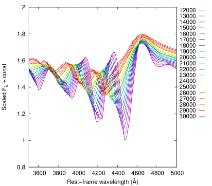
Figure 1: SYN++ models built with $T_{\rm phot}=17000$ K for the W shaped O II blend appearing typically between 3900 and 4500 Å in the pre-maximum spectra Type I SLSNe. Different colors code the models having different $v_{\rm phot}$ values ranging from 10000 to 30000 km s^-1.

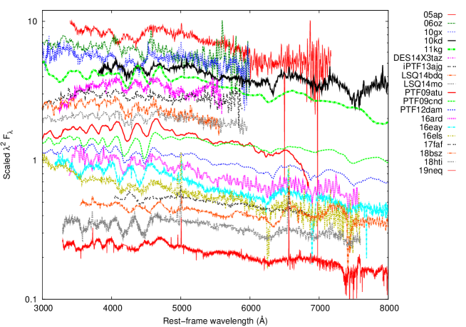
Figure 2: Observed pre-maximum spectra of Type W SLSNe. The colors code the individual objects, and the spectra are shifted vertically for clarity.

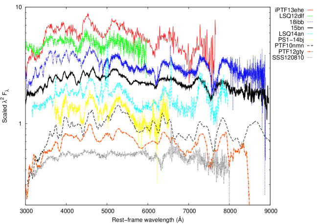
Figure 3: Observed pre-maximum spectra of Type 15bn SLSNe. The colors code the individual objects, and the spectra are shifted vertically for clarity.

However, getting realistic $v_{\rm phot}$ estimates is not a trivial problem, as a typical SLSN spectrum contains broad and heavily blended features instead of isolated and easily identifiable P Cygni profiles. In this case a spectrum synthesis code is required to reliably identify the spectroscopic features and the ejecta composition, but even this method suffers from ambiguity: occasionally, the absorption blends can be fitted equally well with features of different ions (see e.g. Könyves-Tóth et al., 2020). Furthermore, modeling each available spectrum in our sample would be very time consuming. Thus, in Section 4.1 we present a faster and reasonably accurate method by combining spectrum synthesis and cross-correlation (see also e.g. Takáts & Vinkó, 2012; Liu et al., 2017) to estimate the $v_{\rm phot}$ of the 28 SLSNe we studied.

4.1 Methodology

According to e.g. Quimby et al. (2018), and Perley et al. (2019b), a W-shaped absorption feature appearing between $\sim$3900 and $\sim$4500 Å  is typically present in the pre-maximum spectra of Type I SLSNe. It is usually modeled as a blend of O II lines, and assumed to appear in all spectra of Type I SLSNe. Liu et al. (2017) examined a large set of normal and superluminous SNe, and noticed that this W-shaped O II feature can be found in all Type I SLSNe, but missing from the spectrum of normal Type Ic or broad-lined Ic SNe. They proposed the presence/absence of the W-feature as a tool for distinguishing between SLSNe and normal Ic SN events using only pre-maximum spectra.

Motivated by these previous findings, we assumed that the W-shaped feature plays a significant role in the spectrum formation of all SLSNe in our sample. We built a series of SYN++ models (Thomas et al., 2011) containing only O II features (see Figure 1). These models share the same local parameters, e.g. the photospheric temperature ($T_{\rm phot}$) of 17000 K, but have different $v_{\rm phot}$ values ranging from 10000 to 30000 km s^-1, as shown in Figure 1 with different colors. The fixed value of all global ($a_{0}$, $v_{\rm phot}$, $T_{\rm phot}$) and local ($\log\tau$, $v_{\rm min}$, $v_{\rm max}$, $aux$, $T_{\rm exc}$) SYN++ model parameters can be found in Table A2. in the Appendix. Here, we utilize the name global to the parameters referring to the whole model spectrum, and local to the ones fitting the lines of individual elements in the spectrum.

Next, we cross-correlated the O II models to each other using the fxcor task in the onedspec.rv package of IRAF (Image Reduction and Analysis Facility). We chose the model corresponding to $v_{\rm phot}~{}=~{}10000$ km s^-1 as the template spectrum, and computed the cross-correlation velocity differences ($\Delta v_{X}$) between the template and all other model spectra. Then, by comparing $\Delta v_{\rm X}$ with the real velocity differences between the models ($\Delta v_{\rm phot}$), we obtained a formula to convert the velocity differences inferred by fxcor to real, physical velocity differences between the SYN++ models. Having this correction formula we are able to use the cross-correlation method to determine reliable velocities for the observed spectra, despite the well-known issues with applying cross-correlation to spectra with P Cygni features (e.g Takáts & Vinkó, 2012). Our method is similar to the one developed by Liu et al. (2017), but we focused on the more pronounced pre-maximum O II features in the model instead of the Fe II $\lambda 5169$ feature in post-maximum spectra.

Afterwards, we cross-correlated the 28 observed spectra in the sample with the template O II model spectrum (i.e. the one having $v_{\rm phot}~{}=~{}10000$ km s^-1). We derived $v_{\rm phot}$ for the observed spectra by getting $\Delta v_{X}$ from fxcor, then applying the correction formula between $\Delta v_{\rm phot}$ and $\Delta v_{X}$ (see above). As a cross-check, we also plotted together the observed spectra with the SYN++ model having the nearest $v_{\rm phot}$ to the corrected velocity from fxcor (see Section 4.3 and 4.4).

4.2 New subtypes of SLSNe-I

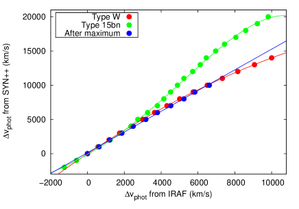
Figure 4: Comparison of the relative velocities between the SYN++ models and the template model given by fxcor ($\Delta v_{\rm X}$, horizontal axis) and the real velocity differences between the model $v_{\rm phot}$ values ($\Delta v_{\rm phot}$, vertical axis). Red and green colors represent the models for the “Type W” and “Type 15bn” subclasses, respectively, while the blue symbols correspond to the post-maximum spectra. The best-fit polynomials are also shown (see text).

Applying the method described above, we found that it did not work for about one-third of the sample, i.e. their derived photospheric velocities turned out to be physically impossible. Closer inspection of those spectra revealed the cause of this inconsistency: the W-shaped O II feature was not present in their spectra at all, therefore, the cross-correlation process did not work properly.

After collecting the spectra without the W-shaped absorption feature, we found that they are similar to each other. The best-observed prototype of these SLSNe is SN 2015bn.

Thus, we define two distinct groups of Type I SLSNe in our sample, characterized by the presence/absence of the W-shaped O II feature between 3900 and 4500 Å. Hereafter we refer them as “Type W” and “Type 15bn” SLSNe (see Table 3).

The observed spectra taken before maximum of all “Type W” SLSNe can be seen in Figure 2, while the same for “Type 15bn” events is shown in Figure 3 with different colors representing each object in the given subclass.

For the latter subclass, we estimated their correct $v_{\rm{phot}}$ values by applying a different SYN++ model template in the cross-correlation process. The formula for correcting their $\Delta v_{\rm{X}}$ to $\Delta v_{\rm{phot}}$ was also re-calculated accordingly.

Further details on the cross-correlation analysis of Type W and Type 15bn SLSNe are given in Section 4.3 and 4.4, respectively.

In Section 4.5, we present the $v_{\rm phot}$ estimates after the maximum for 9 objects in our sample, which had observational data in between +25 and +35 rest-frame days after maximum besides the pre-maximum data. Although e.g. Gal-Yam (2012) and Inserra et al. (2018) defined the Fast and the Slow evolving subgroup of Type I SLSNe by their light curve evolution time-scales, the date of explosion is weakly defined in several cases, thus the rise-time of these SLSNe remains uncertain. Therefore we utilized the photospheric velocity evolution by $\sim$30 days after the maximum for classification (see the details in Section 4.6).

4.3 Type W SLSNe

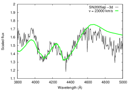
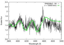
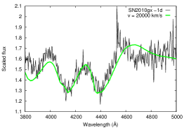
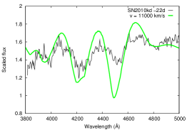
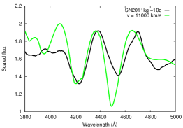
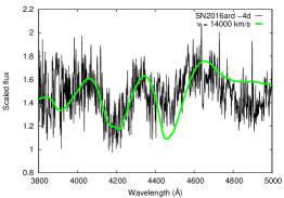
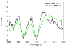
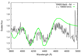
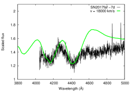
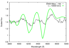
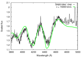
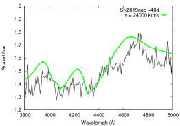
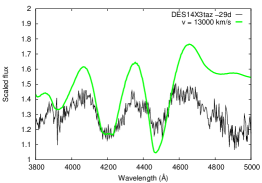
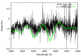
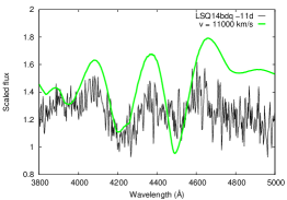
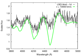
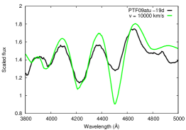
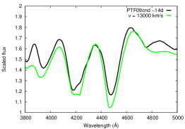
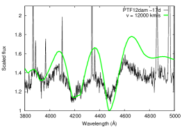
Figure 5: The observed pre-maximum spectra of “Type W” SLSNe (black), together with their best-fit OII model spectra obtained in SYN++ (green).

The real, physical velocity differences ($\Delta v_{\rm phot}$) between the models having $v_{\rm phot}$ ranging from 10000 to 30000 km s^-1 and the template model spectrum of 10000 km s^-1 can be seen in Figure 4 as a function of the velocity difference calculated by the fxcor task in IRAF ($\delta v_{\rm X}$). The data for the “Type W” subclass (red circles) were fitted by a second-order polynomial as

$$\Delta v_{\rm{phot}}~{}=~{}a_{0}~{}+~{}a_{1}\cdot\Delta v_{\rm{X}}~{}+~{}a_{2}\cdot\Delta v_{\rm{X}}^{2},$$ (10)

and obtained $a_{0}=155.01~{}(\pm 82.64)$, $a_{1}=1.68~{}(\pm 0.03)$ and $a_{2}=-2.78\cdot 10^{-5}~{}(\pm 1.63\cdot 10^{-6})$.

Finally, after cross-correlating the observed spectra with the model template, we applied Eq. 10 to infer the final $v_{\rm phot}$ values, which are shown in Table 3, together with epochs of the observations and their rest-frame phases.

In Figure 5, the observed pre-maximum spectra of the “Type W” sample are plotted with black lines, together with the best-fit SYN++ model spectrum (green line) that has the most similar photospheric velocity to the inferred $v_{\rm phot}$. Note that since this analysis aims at measuring only the expansion velocity, the spectra appearing in Fig. 5 are flattened, and neither the continuum, nor the feature depths are fitted. Thus, only the wavelength positions of the features are expected to match.

4.4 Type 15bn SLSNe

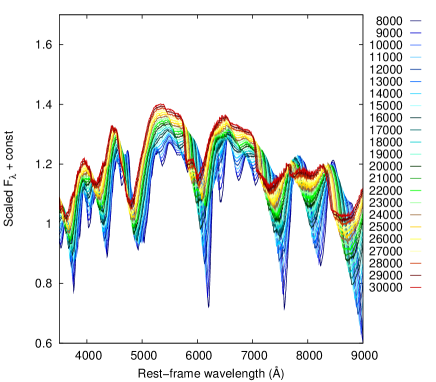
Figure 6: SYN++ models of “Type 15bn” SNe having $T_{\rm phot}$= 11000 K and $v_{\rm phot}$ ranging between 8000 and 30000 km s^-1.

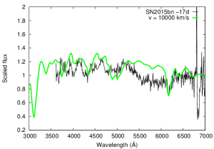
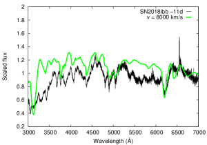
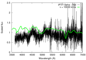
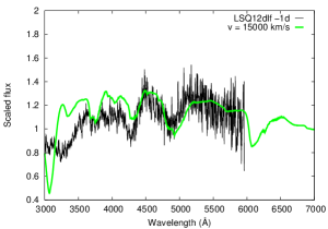
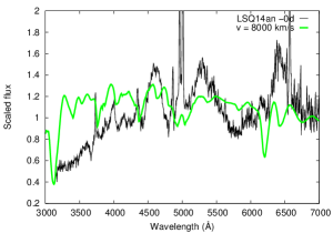
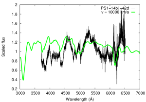
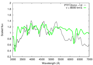
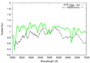
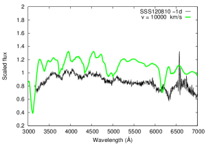
Figure 7: The observed pre-maximum spectra of “Type 15bn” SLSNe (black), together with the Doppler-shifted best-fit model built for SN 2018ibb (green) in accordance with the inferred $v_{\rm phot}$ for each object.

For each object belonging to the “Type 15bn” subclass, the photospheric velocity was determined using the same method as discussed in the previous Section 4.3. However, in this case the modeling of the the whole optical spectrum was necessary to get reliable estimate for $v_{\rm phot}$, since no typical and easily identifiable feature can be found in those spectra in contrast with the “Type W” SLSNe.

Therefore, we built a SYN++ model to describe the spectrum of a well-observed representative of the “Type 15bn” group, which was selected to be SN 2018ibb. The observed spectrum of SN 2018ibb taken at $-11$ rest-frame days relative to maximum light can be seen in the left panel of Figure A1 in the Appendix (black line), together with its best-fit SYN++ model (red line). The single-ion contributions to the overall model spectrum are also presented as orange curves, shifted vertically for better visibility. The photospheric temperature and velocity of the best-fit model is $T_{\rm phot}=11000$ K and $v_{\rm phot}~{}=~{}8000$ km s^-1, respectively. The spectrum contains C II, O I, Mg II, Si II, Ca II, Fe II and Fe III ions. The full set of the global and local parameter values for the SN 2018ibb model can be found in Table A2 in the Appendix.

Thereafter, we synthesized model spectra with the same local and global parameters as the best-fit SYN++ model of the pre-maximum spectrum of SN 2018ibb, but having different $v_{\rm phot}$ in between 8000 and 30000 km s^-1 (see Figure 6). These models were cross-correlated with the one having $v_{\rm phot}~{}=~{}10000$ km s^-1. Then, a similar correction formula between the velocity differences was computed as previously, resulting in

$$\Delta v_{\rm{phot}}~{}=~{}a_{0}~{}+~{}\sum_{n=1}^{4}a_{n}\cdot\Delta v_{\rm{X}}^{n},$$ (11)

with $a_{0}=-128.61~{}(\pm 79.92)$, $a_{1}=1.53~{}(0.06)$, $a_{2}=1.09\cdot 10^{-4}~{}(3.88\cdot 10^{-5})$, $a_{3}=5.45\cdot 10^{-9}~{}(7.44\cdot 10^{-9})$ and $a_{4}=-1.16\cdot 10^{-12}~{}(4.27\cdot 10^{-13})$.

The resulting $\Delta v_{\rm phot}$ values are plotted with green dots in Figure 4, and the best-fit polynomial (Eq. 11.) is shown also with a green line.

Finally, after applying Eq. 11 to the observed pre-maximum spectra in the “Type 15bn” subclass, the $v_{\rm phot}$ velocities are collected in Table 3.

The observed pre-maximum spectra of “Type 15bn” SLSNe are shown in Figure 7 with black lines, together with the best-fit SYN++ model for SN 2018ibb (green) Doppler-shifted to the inferred $v_{\rm phot}$ for each object.

It is seen in Table 3 that SLSNe in the “Type 15bn” group have lower photospheric velocities compared to the “Type W” SLSNe in general. This suggests that “Type 15bn” SLSNe are similar to each other, not only in the appearance of their spectra, but also in their $T_{\rm phot}$ and $v_{\rm phot}$ parameters as well. It is suspected that they are forming a subgroup of SLSNe-I that is different from the “Type W” subclass, because the latter have faster ejecta expansion velocities and hotter photospheres during the pre- and near-maximum phases. In Sections 5 and 6, we discuss additional differences between these two subclasses in details.

4.5 Post-maximum spectra

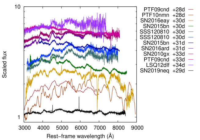
Figure 8: Spectra taken between +25 and +35 days rest-frame phases after maximum light for 9 SLSNe in our sample.

In order to classify the events in our sample into the Fast- or the Slow-evolving subgroup of Type I SLSNe (Inserra et al., 2018), photospheric velocities determined from the spectra taken at $\sim$+30 rest-frame days after maximum are required. By comparing the post-maximum velocities to the $v_{\rm phot}$ estimated near the moment of maximum light, it can be decided unambiguously if a SLSN belongs to the Fast or the Slow SLSNe-I.

From the 28 SLSNe in our sample, 9 possessed post-maximum spectra between +25 and +35 days phase, and both “Type W” and “Type 15bn” objects were represented amongst them,. These spectra are collected and shown in Figure 8.

Table 2: Photospheric velocities before and after the maximum for the 9 SLSNe having post-maximum spectra.

SLSN	Pre-max phase	Pre-max $v_{\rm phot}$	Post-max phase	Post-max $v_{\rm phot}$	W/15bn	Fast/Slow
	(day)	(km s-1)	(day)	(km s-1)
SN2010gx	-1	20371	+33	9926	W	F
SN2015bn	-17	9870	+30	8136	15bn	S
SN2016ard	-4	14398	+31	11585	W	S
SN2016eay	-2	20362	+30	9814	W	F
SN2019neq	-4	23000	+29	9972	W	F
LSQ12dlf	-1	15000	+34	7916	15bn	S
PTF09cnd	-14	13200	+28	7593	W	S
PTF10nmn	-1	7871	+28	4307	15bn	S
SSS120810	-1	9870	+30	8136	15bn	S

From the available post-maximum spectra, the one taken at +30 rest-frame days phase of SN 2015bn was chosen for modeling. It can be seen together with its best-fit SYN++ model in the right panel of Figure A1 in the Appendix, with the same color coding as the model of SN 2018ibb. The best-fit model was found to heve $T_{\rm phot}~{}=~{}9000$ K, and $v_{\rm phot}~{}=~{}8000$ km s^-1, and it contains O I, Na I, Mg II, Si II, Si II v, Ca II and Fe II ions. The ”v” next to Si II refers to the high velocity of this feature. It has higher velocity than $v_{\rm phot}$, as it is formed above the photosphere in the outer regions of the SN ejecta. The parameters of the best-fit SYN++ model can be found in Table A2 in the Appendix.

Since the $v_{\rm phot}$ of an expanding SN atmosphere decreases with time as the ejecta becomes more and more transparent, in case of the post-maximum spectra we utilized and cross-correlated models having lower velocities compared to the models built for the pre-maximum phases.

We created 11 variants of the best-fit model of the +30 days phase spectrum of SN 2015bn, with $v_{\rm phot}$ in between 5000 and 15000 km s^-1 (see Fig. 9). After cross-correlating them, we reached to a similar velocity correction formula, as discussed in Sections 4.3 and 4.4, namely

$$\Delta v_{\rm phot}~{}=~{}a_{0}+a_{1}\Delta v_{\rm X}$$ (12)

with $a_{0}=135.62~{}(\pm 54.81)$ and $a1=1.51(0.01)$. The data as well as the best-fit straight line are shown in Figure 4 with blue color.

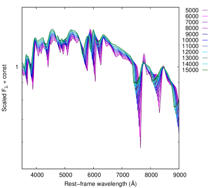
Figure 9: SYN++ models having $T_{\rm phot}~{}=~{}11000$ K, and $v_{\rm phot}$ in between 5000 and 15000 km s^-1 for the spectra taken around $\sim$30 days after maximum.

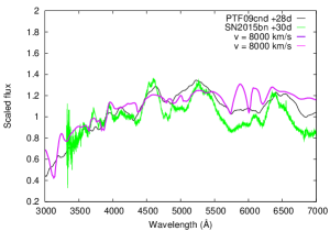
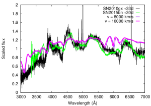
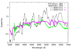
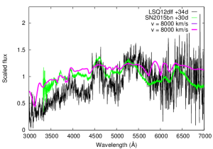
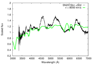
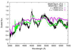
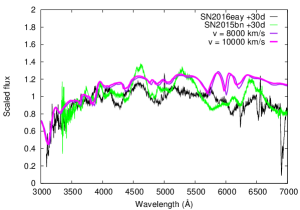
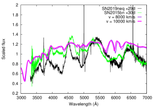
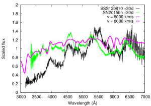
Figure 10: The available post-maximum spectra of 9 SLSNe in our sample (black), with the +30 days phase spectrum of SN 2015bn Doppler-shifted with the velocity difference obtained with IRAF (green). The purple curves refer to the best-fit SYN++ model for SN 2015bn, but Doppler-shifted to $v_{\rm phot}~{}=~{}8000$ km s^-1. The magenta spectrum is the same SYN++ model shifted to the inferred velocity of each SLSN.

Afterwards, we cross-correlated the observed post-maximum spectra with the +30 days phase spectrum of SN 2015bn, instead of a SYN++ model, and then Doppler-shifted them with the $\Delta v_{\rm phot}$ differences from SN 2015bn calculated via fxcor and Eq.12. Figure 10 displays the available post-maximum spectra of 9 SLSNe in our sample (black), together with the +30 days phase spectrum of SN 2015bn Doppler-shifted with the velocity difference obtained with IRAF for each objects (green). The best-fit SYN++ model for SN 2015bn having $v_{\rm phot}~{}=~{}8000$ km s^-1, and the best-fit model referring to the particular SLSN are also plotted with purple and magenta curves, respectively.

The photospheric velocity estimates for the post-maximum phase spectra of the 9 available objects can be found in Table 2.

4.6 Fast/Slow classification

In the case of the 9 events, for which both pre- and post-maximum spectra were available, the classification into the Fast or Slow category was unambiguous. The estimated $v_{\rm phot}$ values before and after maximum can be found in Table 2.

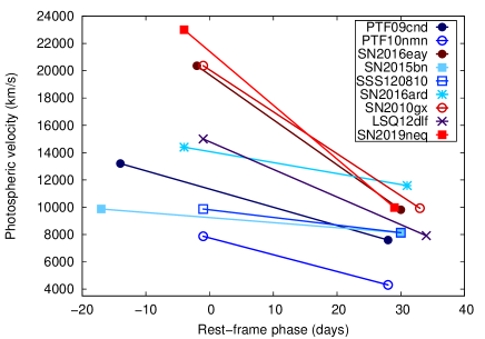
Figure 11: Photospheric velocity evolution of the 9 SLSNe that possessed both pre-maximum and $\sim$30 days post-maximum spectra as well. Red symbols denote objects having $v_{\rm phot}\geq 20000$ km s^-1 near maximum (Fast SLSNe-I), while blue colors code the Slow SLSNe-I exhibiting $v_{\rm phot}\leq 16000$ km s^-1 and almost constant velocity evolution.

Figure 11 displays the photospheric velocity evolution of the 9 SLSNe as a function of rest-frame phase relative to the moment of the maximum light. It is seen that SN 2010gx, SN 2016eay and SN 2019neq shows a factor of 2 higher $v_{\rm phot}$ near maximum than the rest of the sample, which decreases swiftly in the post-maximum phases. By $\sim$30 days after maximum their velocities become similar to those of the other 6 SLSNe. These rapidly evolving objects are plotted with different tones of red in Fig. 11, and they will be referred as Fast (F) Type I SLSNe from now. The fast evolution of these objects is consistent with previous studies (e.g. Pastorello et al., 2010; Inserra et al., 2018; Könyves-Tóth et al., 2020, respectively).

On the contrary, the velocity of PTF09cnd,PTF10nmn, SN 2015bn, SSS120810, SN 2016ard and LSQ12dlf evolves more slowly: it seems to be nearly constant throughout the observed epochs. It is seen also that these 6 objects, plotted with different tones of blue in Fig. 11, are significantly different from the Fast ones in terms of the photospheric velocity evolution, thus, they are to be called Slow (S) SLSNe. This classification is consistent with Inserra et al. (2018), who pointed out that the fast-evolving Type I SLSNe tend to have larger velocity gradients and higher $v_{\rm phot}$ at maximum than Slow SLSNe-I.

It is also seen in Figure 11 that the Fast SLSNe are not only swifter in their $v_{\rm phot}$ evolution, but their near-maximum velocity is significantly higher compared to the Slow ones, in good agreement with Inserra et al. (2018). The photospheric velocity of Fast objects become similar to the $v_{\rm phot}$ of Slow SLSNe by $\sim$30 days after maximum. Therefore, one can distinguish between these two groups of SLSNe-I by comparing their photospheric velocity near maximum. In the followings, we designate the SLSNe-I having $v_{\rm phot}\geq 20000$ km s^-1 as Fast, and the objects with $v_{\rm phot}\leq 16000$ km s^-1 as Slow, as it can be seen in Table 3. Since no post-maximum data of SLSNe-I having $16000\leq v_{\rm phot}\leq 20000$ km s^-1 at maximum were available, 2 objects from our sample, SN 2016els and SN 2017faf, could not be classified into the F or S subgroup unambiguously. Thus, they are referred as ”uncertain” (N) SLSNe-I in Table 3.

In Figure 12, the near-maximum $v_{\rm phot}$ estimates can be seen as a function of the rest-frame light curve (LC) rise time for all SLSNe in our sample. The latter was inferred from Eq.5 using the date of explosion ($t_{0}$) and the moment of the maximum ($t_{max}$) for each object shown in Table 3. “Type W” SLSNe are plotted with filled symbols, while empty circles denote to the “Type 15bn” SLSNe. Red, purple and blue colors code the Fast, the ”uncertain”, and the Slow evolving objects, respectively. It is seen that the SLSNe classified as Fast by their photospheric velocity near maximum are showing short LC rise time scales as well. On the contrary, the objects having $v_{\rm phot}\leq 16000$ km s^-1 at maximum exhibit quite diverse LC evolution time scales. It is also apparent that all “Type 15bn” events (at least those that are analyzed in this paper) belong to the slow-evolving SLSN-I group.

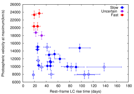
Figure 12: The photospheric velocity estimates for the 28 SLSNe in our sample as a function of the light curve (LC) rise time. Filled dots denote “Type W” objects, while empty circles are the “Type 15bn” SLSNe-I. Red, purple and blue colors code the Fast (F), the ”uncertain” (N), and the Slow (S) categories, respectively.

5 Ejecta mass estimates

The photosheric velocity estimates presented in Section 4 open the door to derive the ejecta mass of the SLSNe in our sample by applying Eq. 7 and 8. To infer the LC rise time ($t_{\rm rise}$), we used the date of the explosion and the moment of maximum light obtained from the Open Supernova Catalogue for all objects (see Table 3).

Ejecta masses calculated from Eq.7 and 8 can be found in Table 3 amongst the estimated $t_{\rm rise}$ and $v_{\rm phot}$ values. We denote the masses inferred from Eq.7 and 8 as $M_{\rm ej}$(7) and $M_{\rm ej}$(8), respectively. We consider their mean, named as $M_{\rm ej}$(mean) in Table 3, as our final mass estimate, and the difference between $M_{\rm ej}(\ref{eq-mej1})$ and $M_{\rm ej}(\ref{eq-mej2})$ as the systematic uncertainty of our ejecta mass estimate: $\sigma_{\rm sys}\approx 0.5\cdot(M_{\rm ej}(\ref{eq-mej1})-M_{\rm ej}(\ref{eq-mej2}))$.

The random errors of $M_{\rm ej}$, $\sigma_{\rm rnd}$, due to the uncertainty of the measured $v_{\rm phot}$ and $t_{\rm rise}$ (estimated as $\delta v_{\rm phot}\sim 1000$ km s^-1 and $\delta t_{\rm tise}\sim 3$ days) were also inferred using error propagation. Both $\sigma_{\rm sys}$ and $\sigma_{\rm rnd}$ are given in Table 3 for each object.

It is seen that the ejecta masses for the whole sample are in the range from 2.9 ($\pm$0.8) to 208 ($\pm$60) $M_{\odot}$. The mean values are $\langle M_{\rm ej}\rangle_{\rm ALL}~{}=~{}42.96\pm 12.50~{}M_{\odot}$ for the 28 events, $\langle M_{\rm ej}\rangle_{\rm S}~{}=~{}49.07\pm 14.80~{}M_{\odot}$ for the Slow SLSNe, and $\langle M_{\rm ej}\rangle_{\rm F}~{}=~{}14.00\pm 6.20~{}M_{\odot}$ for the Fast and uncertain ones.

Figure 13 displays the inferred ejecta masses (blue points) as a function of the light curve rise time scale. It is seen also that the logarithm of the ejecta mass is directly proportional to the logarithm of the LC rise time. It implies that SLSNe having longer rise time tend to have larger ejecta masses compared to the faster evolving objects.

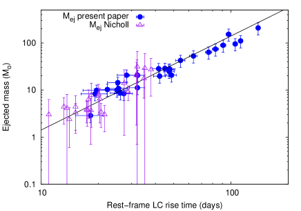
Figure 13: Mean ejecta masses from Table 3 (blue dots) as a function of the light curve rise time, illustrating that faster LC rise implies smaller ejecta mass. The black line represents the $M_{\rm ej}({\rm mean})\sim t_{\rm rise}^{2}$ relation assuming a uniform expansion velocity of $10000$ km s^-1 and $\kappa=0.1$ cm² g^-1 for all objects. The ejecta mass estimates for Type I SLSNe from Nicholl et al. (2015) are plotted with purple triangles. It is seen that these are systematically lower compared to our mean ejecta mass estimates, but obey the same $M_{ej}\sim t_{rise}^{2}$ relation.

Table 3: Results for the light curve rise times and ejecta masses of the studied SLSNe-I.

SLSN	$t_{\rm obs}$[phase]	$t_{\rm rise}$	$M_{\rm ej}$(7)	$M_{\rm ej}$(8)	$M_{\rm ej}$(mean)	$\sigma_{\rm sys}$	$\sigma_{\rm rnd}$	$v_{\rm phot}$	W/15bn	F/S/N
	(days)	(days)	($M_{\odot}$)	($M_{\odot}$)	($M_{\odot}$)	($M_{\odot}$)	($M_{\odot}$)	(km s-1)
SN2005ap	53436 [-3]	19.64	12.74	6.99	9.86	2.87	3.93	23338	W	F
SN2006oz	54061 [-5]	25.58	13.95	7.66	10.80	3.14	3.40	15064	W	S
SN2010gx	55276 [-1]	25.37	18.55	10.19	14.37	4.18	4.48	20371	W	F
SN2010kd	55528 [-22]	47.68	35.75	19.63	27.69	8.06	5.53	11112	W	S
SN2011kg	55926 [-10]	26.17	11.20	6.15	8.68	2.53	2.75	11562	15bn	S
SN2015bn	57082 [-17]	90.88	115.34	63.33	89.34	26.01	13.95	9870	W	S
SN2016ard	57449 [-4]	25.11	12.85	7.06	9.95	2.90	3.20	14398	W	S
SN2016eay	57528 [-2]	19.25	10.68	5.86	8.27	2.41	3.37	20362	W	F
SN2016els	57599 [-5]	22.35	13.26	7.28	10.27	2.99	3.63	18754	W	N
SN2017faf	57934 [-7]	32.26	26.51	14.56	20.54	5.98	5.15	18000	W	N
SN2018bsz	58259 [-16]	76.17	82.09	45.08	63.58	18.51	10.45	10000	W	S
SN2018hti	58428 [-54]	97.08	197.25	108.31	152.78	44.47	18.07	14790	W	S
SN2018ibb	58453 [-11]	112.24	142.61	78.30	110.45	32.15	19.39	8000	15bn	S
SN2019neq	58722 [-4]	28.21	26.69	14.66	20.68	6.02	5.79	23702	W	F
DES14X3taz	57059 [-29]	44.90	37.13	20.39	28.76	8.37	5.72	13017	W	S
iPTF13ajg	56422 [-5]	47.24	32.07	17.61	24.84	7.23	5.15	10155	W	S
iPTF13ehe	56658 [-14]	82.78	95.69	52.54	74.12	21.58	11.92	9870	15bn	S
LSQ12dlf	56149 [-1]	41.59	36.72	20.16	28.44	8.28	5.84	15000	15bn	S
LSQ14an	56660 [0]	18.23	3.70	2.03	2.87	0.83	1.31	7870	15bn	S
LSQ14bdq	56784 [-11]	46.99	35.35	19.41	27.38	7.97	5.49	11314	W	S
LSQ14mo	56694 [-1]	27.29	10.84	5.95	8.40	2.44	2.61	10284	W	S
PS1-14bj	56744 [-42]	138.81	269.11	147.76	208.44	60.67	29.64	9870	15bn	S
PTF09atu	55034 [-19]	42.09	25.46	13.98	19.72	5.74	4.41	10155	W	S
PTF09cnd	55068 [-14]	54.20	54.86	30.12	42.49	12.37	7.36	13199	W	S
PTF10nmn	55384 [-1]	105.19	123.22	67.66	95.44	27.78	17.16	7870	15bn	S
PTF12dam	56072 [-17]	63.39	68.11	37.40	52.75	15.36	8.60	11978	W	S
PTF12gty	56135 [-4]	48.61	26.74	14.68	20.71	6.03	4.70	8000	15bn	S
SSS120810	56135 [-4]	32.18	14.46	7.94	11.20	3.26	3.07	9869	15bn	S

5.1 Comparison with Nicholl et al. (2015)

We compared our results to the calculations of Nicholl et al. (2015), who inferred the ejecta mass of a sample of normal and superluminous supernovae via modeling their bolometric light curves. They utilized an alternative way of using the formula of Arnett (1980) (Eq. 8) by estimating the mean light curve time scale as $t_{\rm m}~{}=~{}0.5\cdot(t_{\rm rise}+t_{\rm dec})$, where $t_{\rm dec}$ is the LC decline time scale. They defined $t_{\rm rise}$, as the time ($t~{}<~{}0$) relative to maximum light ($L_{\rm max}$) at which $L_{\rm griz}~{}=~{}L_{\rm max}/e$, and $t_{\rm dec}$ as as the time ($t~{}>~{}0$) relative to maximum light ($L_{\rm max}$) at which $L_{\rm griz}~{}=~{}L_{\rm max}/e$. This is different from both the original definition of Arnett (1980), who used $t_{\rm m}=\sqrt{2t_{d}t_{h}}$ (cf. Eq.2 and 4), and from our definition of $t_{\rm rise}$ (cf. Eq.5) as well.

Nicholl et al. (2015) utilized a different method to estimate the photospheric velocity as well, based on the Fe II $\lambda$5169 lines in the spectra, obtaining significantly different values from the $v_{\rm phot}$ calculations presented in this study. However, as shown in e.g. Könyves-Tóth et al. (2020), the identification of the Fe II $\lambda$5169 line suffers from ambiguity. Thus, we believe that the modeling of the W-shaped O II feature or the whole spectra provide a more reliable method to estimate the photospheric velocities.

In Figure 13, the ejecta mass calculations of Nicholl et al. (2015) are plotted as a function of their LC rise time scales with purple triangles, in order to compare them to the $M_{\rm ej}$ calculations of this paper (shown with blue dots). It is seen that the ejecta masses published by Nicholl et al. (2015) are systematically smaller, than the $M_{\rm ej}$ values calculated in this study, due to the different method to calculate the light curve rise-time scales, and estimate the photospheric velocities.

6 Discussion

The main goal of this study was to derive the ejecta masses of all SLSNe having public pre-maximum photomeric and spectroscopic observational data in the Open Supernova Catalogue before 2020. To obtain $M_{\rm ej}$, we utilized the formulae of Arnett (1980), summarized in Section 2. Pre- or near-maximum photospheric velocities were crucial to substitute into Eq. 7 and Eq. 8, thus we developed a method to determine the $v_{\rm phot}$ of each object in a fast and efficient way.

We found that the W-shaped O II absorption blend, typically present between $\sim 3900$ and $\sim 4500$ Å in the pre-maximum spectra of Type I SLSNe, is missing from the spectra of 9 SLSNe belonging to our sample. These events are found to be spectroscopically similar to SN 2015bn. Therefore, the studied 28 SLSNe were divided into two subtypes by the presence/absence of the W-shaped absorption: the “Type W” and the “Type 15bn” groups.

The expansion velocities around maximum light were then estimated for both groups by involving SYN++ synthetic models and cross-correlation, as described in Section 4. Furthermore, in order to distinguish between fast- and slow-evolving SLSNe, we repeated this procedure for those events that had public spectra taken around $\sim+30$ rest-frame days after maximum.

The fast or slow evolution of a SLSN can be decided from the photospheric velocity gradient between the $v_{\rm phot}$ measured at the maximum and +30 days phase. Fast SLSNe tend to have larger velocity gradients, while the objects belonging to the Slow group are characterized by much lower velocity gradients or nearly constant photospheric velocities through the observed epochs. This is consistent with the classification scheme of Inserra et al. (2018).

Fast evolving Type I SLSNe can also be distinguished from the Slow evolving objects by their $v_{\rm phot}$ at maximum light: Fast SLSNe-I tend to have $v_{\rm phot}\geq 20000$ km s^-1, while, on the contrary, Slow SLSNe-I usually have $v_{\rm phot}\leq 16000$ km s^-1 instead (see Figure 11).

In some cases, the Fast/Slow classification of a particular object presented in this paper differs from the results of other studies. Five objects out of 28 in our sample (PTF09cnd, PTF10nmn, LSQ14mo, SN 2016ard, and iPTF2016ajg) that were found to be Slow by their $v_{\rm phot}$ evolution are referred to as Fast SLSNe in e.g. Inserra et al. (2018); Chen et al. (2017); Blanchard et al. (2018), and Yu et al. (2017), respectively.

The classification of LSQ12dlf is ambiguous as well: in this paper and according to Yu et al. (2017), it seems to be a slow-evolving SLSN, but Inserra et al. (2018) classified it as a Fast one. The cause of this inconsistency can be found in the different definition of the Fast or Slow evolution: Inserra et al. (2018) found that all objects having $v_{\rm phot}\geq 12000$ km s^-1 at maximum belong to the Fast class according to their definition, while we found the threshold being at $v_{\rm phot}\geq 16000$ km s^-1, near $\sim 20000$ km s^-1 in this study. As displayed in Figure 11, SN 2016ard has $v_{\rm phot}\geq 12000$ km s^-1 with one of the flattest velocity gradients, while LSQ12dlf shows $v_{\rm phot}\leq 16000$ km s^-1 with a medium slope in velocity evolution.

The SLSNe classified into the Fast evolving group by their photospheric velocity measured at maximum are belonging to the Fast Type I SLSN subgroup by their light curve rise times as well. On the contrary, the objects found to be slowly evolving by $v_{\rm phot}$ are quite diverse in $t_{\rm rise}$, ranging in between a few weeks and $\sim 150$ days (see Figure 12).

All SN 2015bn-like SLSNe are classified to the Slow group by their $v_{\rm phot}$, while amongst the “Type W” events both Fast and Slow objects are represented.

The mean and the range of the estimated ejecta masses for the 28 SLSNe in our sample, $\langle M_{\rm ej}\rangle_{\rm ALL}~{}=~{}42.96\pm 12.50~{}M_{\odot}$ between 3 and 208 $M_{\odot}$, are significantly higher than the $M_{\rm ej}$ estimates presented by Nicholl et al. (2015) ($\langle M_{\rm ej}\rangle\sim 10$ $M_{\odot}$, between 3 and 30 $M_{\odot}$ for their sample). The difference is caused by the different method to calculate photospheric velocities and LC time scales.

It is also interesting that the mean mass of the Fast events (including the uncertain ones) in our sample ($\langle M_{\rm ej}\rangle_{\rm F}~{}=~{}14.00\pm 6.20~{}M_{\odot}$) is significantly lower than that of the Slow events ( $\langle M_{\rm ej}\rangle_{\rm S}~{}=~{}49.07\pm 14.80~{}M_{\odot}$). At first glance this might suggest that the physical cause of the Fast/Slow dichotomy could be related to the amount of the ejected envelope. However, as the sample is still very poor (only 28 objects), more data are strongly needed to be able to draw more reliable conclusion.

7 Summary

We have presented photospheric velocity estimates and ejecta mass calculations of a sample containing 28 Type I superluminous supernovae having publicly available photometric and spectroscopic data in the Open Supernova Catalogue (Guillochon et al., 2017).

We utilized the formulae of the radiation-diffusion model of Arnett (1980) to estimate the ejecta masses. The LC rise time and the photospheric velocity before or near the luminosity maximum was necessary to obtain $M_{\rm ej}$ values.

The photospheric velocities of the sample SLSNe were estimated utilizing a method by combining the spectrum modeling with cross-correlation, similar to Takáts & Vinkó (2012). It was found that the W shaped O II absorption blend, typically present in the pre-maximum spectra of Type I SLSNe is missing from the spectra of several objects that otherwise have very similar features to SN 2015bn. Thus, two groups of the sample SLSNe were created (called “Type W” and “Type 15bn”), and their $v_{\rm phot}$ values were obtained using different SYN++ model spectra as templates in the cross-correlation.

Post-maximum $v_{\rm phot}$ values of 9 SLSNe with available spectra were also estimated in a similar way in order to to classify these events into the Fast or the Slow SLSN subtypes by calculating the velocity gradients between the maximum, and +30 rest-frame days. Fast SLSNe showed considerably higher velocity gradiens than Slow ones, in good agreement with Inserra et al. (2018).

These calculations also confirmed that Fast SLSNe generally show higher velocities close to maximum than Slow events. This allowed us to classify other SLSNe in our sample that did not have public spectra around +30 days. Thus, we considered the SLSNe having $v_{\rm phot}\geq 20000$ km s^-1 near maximum as Fast (F), and the events with $v_{\rm phot}\leq 16000$ km s^-1 as Slow (S) events.

Amongst the studied SLSNe, the Fast evolving objects defined by the photospheric velocities were revealed to show a rapidly evolving light curve with a short LC rise time as well. On the contrary, Slow evolving events having lower $v_{\rm phot}$ had more diverse LC rise time scales, ranging from a few weeks to $\sim$150 days. It was also found that all “Type 15bn” events belong to the Slow evolving SLSN-I subgroup defined by $v_{\rm phot}$, while “Type W” objects were represented in both the Fast and Slow groups.

Ejecta mass calculations of the SLSNe in our sample were carried our using Eq. 7 and 8, resulting in masses within a range of 2.9 ($\pm 0.8$) - 208 ($\pm 61$) $M_{\odot}$, having a mean of $\langle M_{\rm ej}\rangle=42.96\pm 12.50~{}M_{\odot}$. This is significantly larger than the $\langle M_{\rm ej}\rangle$ calculated by Nicholl et al. (2015), who obtained $\langle M_{\rm ej}\rangle\sim 10~{}M_{\odot}$ between 3 and 30 $M_{\odot}$ for a different sample of SLSNe I with different methods to estimate the photospheric velocities and LC evolution timescales.

The mean ejecta mass of Slow SLSNe in our sample ($\sim 49\pm 15~{}M_{\odot}$) seems to be higher than that of the Fast ones ($\sim 14\pm 6~{}M_{\odot}$), suggesting a physical link between the Fast/Slow dichotomy and the ejecta mass. However, since it is based on only 28 (24 Slow and 4 Fast) objects, more data are inevitable for a more reliable conclusion.

Our ejecta mass estimates further strengthen the long-standing concept that SLSNe probably originate from a range of moderately massive to very massive progenitors, and their (still uncertain) explosion mechanism is able to eject large amount of their envelope mass.

8 Appendix

Table A1 summarizes the selection process of out sample. Here, we describe in details the cause of removing 13 SLSNe-I having pre-maximum spectra.

• The pre-maximum spectra of SN 2019szu, SCP-06F6 and OGLE15qz were so noisy that spectral features could not be identified at all.

• DES15E2mlf, SNLS-06D4eu and SNLS-07D2bv were observed only in the UV bands up to 3000 Å.

• The spectra taken of SN 2010md, PTF10vqv, SN 2016aj, and SN 2010uhf did not contain the typical SLSN-I spectral features, or the W-like absorption between 3900 and 4500 Å, which is usually present in the pre-maximum spectra of SLSNe-I.

• The selected spectrum of SN 2007bi was actually taken after the maximum.

• SN 2015L, the most luminous ”SLSN” ever seen is presumably a tidal disruption event (e.g. Leloudas et al., 2016; Margutti et al., 2017; Coughlin & Armitage, 2018). If we assume it to be a SLSN, it interacts so robustly that the photosphere is not even visible, thus it is impossible to estimate the photospheric velocity in the maximum.

• SN 2017gir had a spectrum more similar to a Type II SLSN.

In Fig. A1, the SYN++ modeling of the -11 days phase spectrum of SN 2018ibb (Type 15bn; left panel) and the +30 days phase spectrum of SN 2015bn (right panel) is plotted.

Table A2 summarizes the global and local SYN++ parameters obtained for Type W, Type 15bn, and post-maximum SLSN spectra.

Table A1: SLSNe removed from our sample.

Reason for exclusion [number]	SLSN
SLSNe-II [18]	SN2006gy, SN1000+0216, SN2008am, SN2008es, CSS121015:004244+132827, PTF12mkp, SN2013hx, PS15br,
	LSQ15abl, SN2016aps, SN2016ezh, SN2016jhm, SN2016jhn, SN2017bcc, SN2017egm, SN2018jkq, SN2019cmv,
	SN2019meh
Without pre-maximum spectra [39]	SN2213-1745, SDSS-II SN 2538, SDSS-II SN17789, SN2009cb, SN2009jh, PTF10bfz, PTF10bjp, PS1-10pm, PS1-10ky,
	PS1-11tt, PS1-10ahf, SN2010hy, PS1-10awh, PTF10aagc, PS1-10bzj, PS1-11ap, SN2011ke, PS1-11afv, PTF11hrq,
	SN2011kl, SN2011kf, SN2012il, PTF12mxx, SN2013dg, SN2013hy, CSS130912:025702-001844, PS15cjz,
	OGLE15sd, PS16yj, iPTF16bad, DES16C2nm, AT2016jho, SN2017jan, DES17C3gyp, SN2018bgv, SN2018gkz,
	SN2018lfd, SN2019meh, SN2019szu
Problem with spectra [13]	SN 2019szu, SCP-06F6, OGLE15qz, DES15E2mlf, SNLS-06D4eu, SNLS-07D2bv, SN 2010md, PTF10vqv, SN 2016aj,
	SN 2010uhf, SN 2007bi, SN 2015L, SN 2017gir

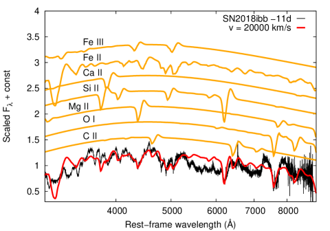
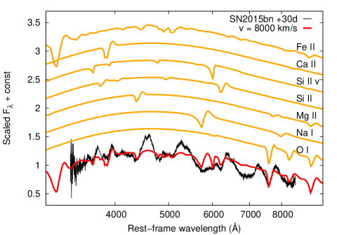
Figure A1: Left panel: The -11 days rest-frame phase spectrum of SN 2018ibb (black), belonging to the Type 15bn group of SLSNe-I together with its best-fit model obtained in SYN++ (red). Single ion contributions to the overall model spectrum are plotted with orange, shifted vertically to guide the eye. Right panel: The +30 days phase spectrum of SN 2015bn plotted the same way as the figure on the left.

Table A2: Global and local SYN++ parameters for the studied Type W, Type 15bn, and post-maximum phase SLSNe.

Type W SLSNe
Global parameters
$a_{0}$	$v_{\rm phot}$	$T_{\rm phot}$
	(km s-1)	($10^{3}$ K)
1.0	10000-30000	15000
Local parameters
Element	$\log\tau$	$v_{\rm min}$	$v_{\rm max}$	$aux$	$T_{\rm exc}$
		($10^{3}$ km s-1)	($10^{3}$ km s-1)	($10^{3}$ km s-1)	($10^{3}$ K)
O II	-2.0	$v_{\rm phot}$	50.0	2.0	15.0
Type 15bn SLSNe
Global parameters
$a_{0}$	$v_{\rm phot}$	$T_{\rm phot}$
	(km s-1)	($10^{3}$ K)
0.7	8000-30000	11000
Local parameters
Element	$\log\tau$	$v_{\rm min}$	$v_{\rm max}$	$aux$	$T_{\rm exc}$
		($10^{3}$ km s-1)	($10^{3}$ km s-1)	($10^{3}$ km s-1)	($10^{3}$ K)
C II	-1.4	$v_{\rm phot}$	50.0	1.0	10.0
O I	0.3	$v_{\rm phot}$	50.0	1.0	10.0
Mg II	0.0	$v_{\rm phot}$	50.0	1.0	10.0
Si II	0.5	$v_{\rm phot}$	50.0	1.0	10.0
Ca II	0.0	$v_{\rm phot}$	50.0	1.0	10.0
Fe II	0.0	$v_{\rm phot}$	50.0	1.0	12.0
Fe III	-0.5	$v_{\rm phot}$	50.0	1.0	10.0
SLSNe after maximum
Global parameters
$a_{0}$	$v_{\rm phot}$	$T_{\rm phot}$
	(km s-1)	($10^{3}$ K)
0.7	5000-15000	9000
Local parameters
Element	$\log\tau$	$v_{\rm min}$	$v_{\rm max}$	$aux$	$T_{\rm exc}$
		($10^{3}$ km s-1)	($10^{3}$ km s-1)	($10^{3}$ km s-1)	($10^{3}$ K)
O I	0.1	$v_{\rm phot}$	50.0	1.0	10.0
Na I	-0.5	$v_{\rm phot}$	50.0	4.0	10.0
Mg II	-0.5	$v_{\rm phot}$	50.0	1.0	10.0
Si II	-0.3	$v_{\rm phot}$	50.0	1.0	10.0
Si II v	0.7	17.0	50.0	3.0	10.0
Ca II	0.0	$v_{\rm phot}$	50.0	1.0	10.0
Fe II	-0.5	$v_{\rm phot}$	50.0	1.0	12.0

References

- Anderson et al. (2018) Anderson, J. P., Pessi, P. J., Dessart, L., et al. 2018, A&A, 620, A67
- Angus et al. (2016) Angus, C. R., Levan, A. J., Perley, D. A., et al. 2016, MNRAS, 458, 84
- Angus et al. (2019) Angus, C. R., Smith, M., Sullivan, M., et al. 2019, MNRAS, 487, 2215
- Arabsalmani et al. (2019) Arabsalmani, M., Roychowdhury, S., Renaud, F., et al. 2019, ApJ, 882, 31
- Arnett (1980) Arnett, W. D. 1980, ApJ, 237, 541
- Arnett (1982) Arnett, W. D. 1982, ApJ, 253, 785
- Arnett & Fu (1989) Arnett, W. D. & Fu, A. 1989, ApJ, 340, 396
- Bassett et al. (2006) Bassett, B., Becker, A., Brewington, H., et al. 2006, Central Bureau Electronic Telegrams, 762
- Benetti et al. (2014) Benetti, S., Nicholl, M., Cappellaro, E., et al. 2014, MNRAS, 441, 289
- Benitez et al. (2014) Benitez, S., Polshaw, J., Inserra, C., et al. 2014, The Astronomer’s Telegram, 6118
- Blanchard et al. (2018) Blanchard, P., Nicholl, M., Chornock, R., et al. 2018, The Astronomer’s Telegram, 11790
- Bose et al. (2018) Bose, S., Dong, S., Pastorello, A., et al. 2018, ApJ, 853, 57
- Branch & Wheeler (2017) Branch, D. & Wheeler, J. C. 2017, Supernova Explosions: Astronomy and Astrophysics Library, ISBN 978-3-662-55052-6. Springer-Verlag GmbH Germany, 2017
- Brown et al. (2014) Brown, P. J., Breeveld, A. A., Holland, S., et al. 2014, Ap&SS, 354, 89
- Burke et al. (2018) Burke, J., Hiramatsu, D., Arcavi, I., et al. 2018, Transient Name Server Classification Report, 2018-1719
- Castander et al. (2015) Castander, F. J., Casas, R., Garcia-Alvarez, D., et al. 2015, The Astronomer’s Telegram, 7190
- Chatzopoulos et al. (2012) Chatzopoulos, E., Wheeler, J. C., & Vinko, J. 2012, ApJ, 746, 121
- Chatzopoulos et al. (2013) Chatzopoulos, E., Wheeler, J. C., Vinko, J., et al. 2013, ApJ, 773, 76
- Chandra et al. (2009) Chandra, P., Ofek, E. O., Frail, D. A., et al. 2009, The Astronomer’s Telegram, 2241
- Chen et al. (2017) Chen, T.-W., Nicholl, M., Smartt, S. J., et al. 2017, A&A, 602, A9
- Chornock et al. (2016) Chornock, R., Bhirombhakdi, K., Katebi, R., et al. 2016, The Astronomer’s Telegram, 8790
- Coughlin & Armitage (2018) Coughlin, E. R. & Armitage, P. J. 2018, MNRAS, 474, 3857
- De Cia et al. (2018) De Cia, A., Gal-Yam, A., Rubin, A., et al. 2018, ApJ, 860, 100
- Dessart (2019) Dessart, L. 2019, A&A, 621, A141
- Drake et al. (2009) Drake, A. J., Djorgovski, S. G., Mahabal, A., et al. 2009, ApJ, 696, 870
- Gal-Yam (2009) Gal-Yam, A. 2009, GALEX Proposal, 35
- Gal-Yam (2012) Gal-Yam, A. 2012, Science, 337, 927
- Gal-Yam (2019) Gal-Yam, A. 2019, ARA&A, 57, 305
- Gal-Yam (2019b) Gal-Yam, A. 2019, ApJ, 882, 102
- Green (2006) Green, D. W. E. 2006, Central Bureau Electronic Telegrams, 762
- Guillochon et al. (2017) Guillochon, J., Parrent, J., Kelley, L. Z., et al. 2017, ApJ, 835, 64
- Hatsukade et al. (2018) Hatsukade, B., Tominaga, N., Hayashi, M., et al. 2018, ApJ, 857, 72
- Hatsukade et al. (2020) Hatsukade, B., Morokuma-Matsui, K., Hayashi, M., et al. 2020, PASJ, doi:10.1093/pasj/psaa052
- Inserra et al. (2017) Inserra, C., Nicholl, M., Chen, T.-W., et al. 2017, MNRAS, 468, 4642
- Inserra et al. (2018) Inserra, C., Prajs, S., Gutierrez, C. P., et al. 2018, ApJ, 854, 175
- Izzo et al. (2018) Izzo, L., Thöne, C. C., García-Benito, R., et al. 2018, A&A, 610, A11
- Japelj et al. (2016) Japelj, J., Vergani, S. D., Salvaterra, R., et al. 2016, A&A, 593, A115
- Kangas et al. (2016) Kangas, T., Elias-Rosa, N., Lundqvist, P., et al. 2016, The Astronomer’s Telegram, 9071
- Kangas et al. (2017) Kangas, T., Blagorodnova, N., Mattila, S., et al. 2017, MNRAS, 469, 1246
- Kasen et al. (2011) Kasen, D., Woosley, S. E., & Heger, A. 2011, ApJ, 734, 102
- Khatami & Kasen (2019) Khatami, D. K. & Kasen, D. N. 2019, ApJ, 878, 56
- Könyves-Tóth et al. (2020) Könyves-Tóth, R., Thomas, B. P., Vinkó, J., et al. 2020, ApJ, 900, 73
- Kumar et al. (2020) Kumar, A., Pandey, S. B., Konyves-Toth, R., et al. 2020, ApJ, 892, 28
- Leget et al. (2014) Leget, P.-F., Le Guillou, L., Fleury, M., et al. 2014, The Astronomer’s Telegram, 5718
- Le Guillou et al. (2015) Le Guillou, L., Mitra, A., Baumont, S., et al. 2015, The Astronomer’s Telegram, 7102
- Leloudas et al. (2016) Leloudas, G., Fraser, M., Stone, N. C., et al. 2016, Nature Astronomy, 1, 0002
- Leloudas et al. (2012) Leloudas, G., Chatzopoulos, E., Dilday, B., et al. 2012, A&A, 541, A129
- Leloudas et al. (2014) Leloudas, G., Ergon, M., Taddia, F., et al. 2014, The Astronomer’s Telegram, 5839
- Leloudas et al. (2015) Leloudas, G., Schulze, S., Krühler, T., et al. 2015, MNRAS, 449, 917
- Lennarz et al. (2012) Lennarz, D., Altmann, D., & Wiebusch, C. 2012, A&A, 538, A120
- Levan et al. (2013) Levan, A. J., Read, A. M., Metzger, B. D., et al. 2013, ApJ, 771, 136
- Liu et al. (2017) Liu, Y.-Q., Modjaz, M., & Bianco, F. B. 2017, ApJ, 845, 85
- Lunnan et al. (2013) Lunnan, R., Chornock, R., Berger, E., et al. 2013, ApJ, 771, 97
- Lunnan et al. (2014) Lunnan, R., Chornock, R., Berger, E., et al. 2014, ApJ, 787, 138
- Lunnan et al. (2016) Lunnan, R., Chornock, R., Berger, E., et al. 2016, ApJ, 831, 144
- Lunnan et al. (2018) Lunnan, R., Chornock, R., Berger, E., et al. 2018, ApJ, 852, 81
- Maeda et al. (2007) Maeda, K., Tanaka, M., Nomoto, K., et al. 2007, ApJ, 666, 1069
- Margutti et al. (2017) Margutti, R., Metzger, B. D., Chornock, R., et al. 2017, ApJ, 836, 25
- Modjaz et al. (2005) Modjaz, M., Kirshner, R., Challis, P., et al. 2005, IAU Circ., 8492
- Nagy et al. (2014) Nagy, A. P., Ordasi, A., Vinkó, J., et al. 2014, A&A, 571, A77
- Nagy & Vinkó (2016) Nagy, A. P. & Vinkó, J. 2016, A&A, 589, A53
- Nagy (2018) Nagy, A. P. 2018, ApJ, 862, 143
- Neill et al. (2011) Neill, J. D., Sullivan, M., Gal-Yam, A., et al. 2011, ApJ, 727, 15
- Nicholl et al. (2014) Nicholl, M., Smartt, S. J., Jerkstrand, A., et al. 2014, MNRAS, 444, 2096
- Nicholl et al. (2015b) Nicholl, M., Smartt, S. J., Jerkstrand, A., et al. 2015, ApJ, 807, L18
- Nicholl et al. (2015) Nicholl, M., Smartt, S. J., Jerkstrand, A., et al. 2015, MNRAS, 452, 3869
- Nicholl et al. (2016) Nicholl, M., Berger, E., Smartt, S. J., et al. 2016, ApJ, 826, 39
- Nicholl et al. (2016B) Nicholl, M., Berger, E., Margutti, R., et al. 2016, ApJ, 828, L18
- Nicholl et al. (2017) Nicholl, M., Berger, E., Margutti, R., et al. 2017, ApJ, 835, L8
- Nordin et al. (2019) Nordin, J., Brinnel, V., Giomi, M., et al. 2019, Transient Name Server Discovery Report, 2019-1472
- Ofek et al. (2013) Ofek, E. O., Fox, D., Cenko, S. B., et al. 2013, ApJ, 763, 42
- Pastorello et al. (2010) Pastorello, A., Smartt, S. J., Botticella, M. T., et al. 2010, ApJ, 724, L16
- Pastorello et al. (2010b) Pastorello, A., Smartt, S. J., Botticella, M. T., et al. 2010, Central Bureau Electronic Telegrams, 2413
- Pastorello et al. (2017) Pastorello, A., Benetti, S., Cappellaro, E., et al. 2017, The Astronomer’s Telegram, 10554
- Perley et al. (2016) Perley, D. A., Quimby, R. M., Yan, L., et al. 2016, ApJ, 830, 13
- Perley (2019) Perley, D. A. 2019, Transient Name Server Classification Report, 2019-1646
- Perley et al. (2019b) Perley, D. A., Yan, L., Gal-Yam, A., et al. 2019, Transient Name Server AstroNote, 79, 1
- Pinto & Eastman (2000a) Pinto, P. A. & Eastman, R. G. 2000, ApJ, 530, 744
- Pinto & Eastman (2000b) Pinto, P. A. & Eastman, R. G. 2000, ApJ, 530, 757
- Piro & Nakar (2014) Piro, A. L. & Nakar, E. 2014, ApJ, 784, 85
- Popov (1993) Popov, D. V. 1993, ApJ, 414, 712
- Puckett et al. (2005) Puckett, T., Crowley, T., Quimby, R., et al. 2005, IAU Circ., 8492
- Pursiainen et al. (2018) Pursiainen, M., Castro-Segura, N., Smith, M., et al. 2018, Transient Name Server Classification Report, 2018-2184
- Quimby et al. (2007) Quimby, R. M., Aldering, G., Wheeler, J. C., et al. 2007, ApJ, 668, L99
- Quimby et al. (2012) Quimby, R. M., Arcavi, I., Sternberg, A., et al. 2012, The Astronomer’s Telegram, 4121
- Quimby et al. (2013) Quimby, R. M., Gal-Yam, A., Arcavi, I., et al. 2013, Central Bureau Electronic Telegrams, 3464
- Quimby et al. (2018) Quimby, R. M., De Cia, A., Gal-Yam, A., et al. 2018, ApJ, 855, 2
- Sako et al. (2018) Sako, M., Bassett, B., Becker, A. C., et al. 2018, PASP, 130, 064002
- Schlafly & Finkbeiner (2011) Schlafly, E. F. & Finkbeiner, D. P. 2011, ApJ, 737, 103
- Schulze et al. (2018) Schulze, S., Krühler, T., Leloudas, G., et al. 2018, MNRAS, 473, 1258
- Shivvers et al. (2019) Shivvers, I., Filippenko, A. V., Silverman, J. M., et al. 2019, MNRAS, 482, 1545
- Smartt et al. (2012) Smartt, S. J., Inserra, C., Fraser, M., et al. 2012, The Astronomer’s Telegram, 4299
- Smartt et al. (2015) Smartt, S. J., Valenti, S., Fraser, M., et al. 2015, A&A, 579, A40
- Smith et al. (2007) Smith, N., Li, W., Foley, R. J., et al. 2007, ApJ, 666, 1116
- Smith et al. (2016) Smith, M., Sullivan, M., D’Andrea, C. B., et al. 2016, ApJ, 818, L8
- Takáts & Vinkó (2012) Takáts, K. & Vinkó, J. 2012, MNRAS, 419, 2783
- Thomas et al. (2011) Thomas, R. C., Nugent, P. E., & Meza, J. C. 2011, PASP, 123, 237
- Tonry et al. (2018) Tonry, J., Denneau, L., Heinze, A., et al. 2018, Transient Name Server Discovery Report, 2018-1680
- Valenti et al. (2008) Valenti, S., Benetti, S., Cappellaro, E., et al. 2008, MNRAS, 383, 1485
- Vreeswijk et al. (2014) Vreeswijk, P. M., Savaglio, S., Gal-Yam, A., et al. 2014, ApJ, 797, 24
- Wright et al. (2012) Wright, D., Cellier-Holzem, F., Inserra, C., et al. 2012, The Astronomer’s Telegram, 4313
- Yan et al. (2015) Yan, L., Quimby, R., Ofek, E., et al. 2015, ApJ, 814, 108
- Yan et al. (2017) Yan, L., Lunnan, R., Perley, D. A., et al. 2017, ApJ, 848, 6
- Yan et al. (2018) Yan, L., Perley, D. A., De Cia, A., et al. 2018, ApJ, 858, 91
- Yaron & Gal-Yam (2012) Yaron, O. & Gal-Yam, A. 2012, PASP, 124, 668
- Yu et al. (2017) Yu, Y.-W., Zhu, J.-P., Li, S.-Z., et al. 2017, ApJ, 840, 12