c-lasso: a Python package for constrained sparse regression and classification

Summary

We introduce c-lasso, a Python package that enables sparse and robust linear regression and classification with linear equality constraints. The underlying statistical forward model is assumed to be of the following form:

$$y=X\beta+\sigma\epsilon\qquad\textrm{subject to}\qquad C\beta=0$$

Here, $X\in\mathbb{R}^{n\times d}$ is a given design matrix and the vector $y\in\mathbb{R}^{n}$ is a continuous or binary response vector. The matrix $C$ is a general constraint matrix. The vector $\beta\in\mathbb{R}^{d}$ contains the unknown coefficients and $\sigma$ an unknown scale. Prominent use cases are (sparse) log-contrast regression with compositional data $X$, requiring the constraint $1_{d}^{T}\beta=0$ (Aitchion and Bacon-Shone 1984) and the Generalized Lasso which is a special case of the described problem (see, e.g, (James, Paulson, and Rusmevichientong 2020), Example 3). The c-lasso package provides estimators for inferring unknown coefficients and scale (i.e., perspective M-estimators (Combettes and Müller 2020a)) of the form

$$\min_{\beta\in\mathbb{R}^{d},\sigma\in\mathbb{R}_{0}}f\left(X\beta-y,{\sigma}\right)+\lambda\left\lVert\beta\right\rVert_{1}\qquad\textrm{subject to}\qquad C\beta=0$$

for several convex loss functions $f(\cdot,\cdot)$. This includes the constrained Lasso, the constrained scaled Lasso, and sparse Huber M-estimators with linear equality constraints.

Statement of need

Currently, there is no Python package available that can solve these ubiquitous statistical estimation problems in a fast and efficient manner. c-lasso provides algorithmic strategies, including path and proximal splitting algorithms, to solve the underlying convex optimization problems with provable convergence guarantees. The c-lasso package is intended to fill the gap between popular Python tools such as https://scikit-learn.org/stable/https://doi.orgscikit-learn which cannot solve these constrained problems and general-purpose optimization solvers such as https://www.cvxpy.orghttps://doi.orgcvxpy that do not scale well for these problems and/or are inaccurate. c-lasso can solve the estimation problems at a single regularization level, across an entire regularization path, and includes three model selection strategies for determining the regularization parameter: a theoretically-derived fixed regularization, k-fold cross-validation, and stability selection. We show several use cases of the package, including an application of sparse log-contrast regression tasks for compositional microbiome data, and highlight the seamless integration into R via https://rstudio.github.io/reticulate/https://doi.orgreticulate.

Functionalities

Installation and problem instantiation

c-lasso is available on pip and can be installed in the shell using

pip install c-lasso

The central object in the c-lasso package is the instantiation of a c-lasso problem.

# Import the main class of the packagefrom classo import classo_problem# Define a c-lasso problem instance with default setting, # given data X, y, and constraints C.problem  = classo_problem(X,y,C)

We next describe what type of problem instances are available and how to solve them.

Statistical problem formulations

Depending on the type of and the prior assumptions on the data, the noise $\epsilon$, and the model parameters, c-lasso allows for different estimation problem formulations. More specifically, the package can solve the following four regression-type and two classification-type formulations:

R1 Standard constrained Lasso regression:

$$\min_{\beta\in\mathbb{R}^{d}}\left\lVert X\beta-y\right\rVert^{2}+\lambda\left\lVert\beta\right\rVert_{1}\qquad\textrm{subject to}\qquad C\beta=0$$

This is the standard Lasso problem with linear equality constraints on the $\beta$ vector. The objective function combines Least-Squares (LS) for model fitting with the $L_{1}$-norm penalty for sparsity.

# Formulation R1problem.formulation.huber = Falseproblem.formulation.concomitant = Falseproblem.formulation.classification = False

R2 Contrained sparse Huber regression:

$$\min_{\beta\in\mathbb{R}^{d}}h_{\rho}(X\beta-y)+\lambda\left\lVert\beta\right\rVert_{1}\qquad\textrm{subject to}\qquad C\beta=0$$

This regression problem uses the https://en.wikipedia.org/wiki/Huber_losshttps://doi.orgHuber loss $h_{\rho}$ as objective function for robust model fitting with an $L_{1}$ penalty and linear equality constraints on the $\beta$ vector. The default parameter $\rho$ is set to $1.345$ (Huber 1981).

# Formulation R2problem.formulation.huber = Trueproblem.formulation.concomitant = Falseproblem.formulation.classification = False

R3 Contrained scaled Lasso regression:

$$\min_{\beta\in\mathbb{R}^{d},\sigma\in\mathbb{R}_{0}}\frac{\left\lVert X\beta-y\right\rVert^{2}}{\sigma}+\frac{n}{2}\sigma+\lambda\left\lVert\beta\right\rVert_{1}\qquad\textrm{subject to}\qquad C\beta=0$$

This formulation is the default problem formulation in c-lasso. It is similar to R1 but allows for joint estimation of the (constrained) $\beta$ vector and the standard deviation $\sigma$ in a concomitant fashion (Combettes and Müller 2020a; Combettes and Müller 2020b).

# Formulation R3problem.formulation.huber = Falseproblem.formulation.concomitant = Trueproblem.formulation.classification = False

R4 Contrained sparse Huber regression with concomitant scale estimation:

$$\min_{\beta\in\mathbb{R}^{d},\sigma\in\mathbb{R}_{0}}\left(h_{\rho}\left(\frac{X\beta-y}{\sigma}\right)+n\right)\sigma+\lambda\left\lVert\beta\right\rVert_{1}\qquad\textrm{subject to}\qquad C\beta=0$$

This formulation combines R2 and R3 allowing robust joint estimation of the (constrained) $\beta$ vector and the scale $\sigma$ in a concomitant fashion (Combettes and Müller 2020a; Combettes and Müller 2020b).

# Formulation R4problem.formulation.huber = Trueproblem.formulation.concomitant = Trueproblem.formulation.classification = False

C1 Contrained sparse classification with Square Hinge loss:

$$\min_{\beta\in\mathbb{R}^{d}}\sum_{i=1}^{n}l(y_{i}x_{i}^{\top}\beta)+\lambda\left\lVert\beta\right\rVert_{1}\qquad\textrm{subject to}\qquad C\beta=0$$

where $x_{i}$ denotes the $i^{th}$ row of $X$, $y_{i}\in\{-1,1\}$, and $l(\cdot)$ is defined for $r\in\mathbb{R}$ as:

$$l(r)=\begin{cases}(1-r)^{2}&if\quad r\leq 1\\ 0&if\quad r\geq 1\end{cases}$$

This formulation is similar to R1 but adapted for classification tasks using the Square Hinge loss with (constrained) sparse $\beta$ vector estimation (Lee and Lin 2013).

# Formulation C1problem.formulation.huber = Falseproblem.formulation.concomitant = Falseproblem.formulation.classification = True

C2 Contrained sparse classification with Huberized Square Hinge loss:

$$\min_{\beta\in\mathbb{R}^{d}}\sum_{i=1}^{n}l_{\rho}(y_{i}x_{i}^{\top}\beta)+\lambda\left\lVert\beta\right\rVert_{1}\qquad\textrm{subject to}\qquad C\beta=0\,.$$

This formulation is similar to C1 but uses the Huberized Square Hinge loss $l_{\rho}$ for robust classification with (constrained) sparse $\beta$ vector estimation (Rosset and Zhu 2007):

$$l_{\rho}(r)=\begin{cases}(1-r)^{2}&if\quad\rho\leq r\leq 1\\ (1-\rho)(1+\rho-2r)&if\quad r\leq\rho\\ 0&if\quad r\geq 1\end{cases}$$

This formulation can be selected in c-lasso as follows:

# Formulation C2problem.formulation.huber = Trueproblem.formulation.concomitant = Falseproblem.formulation.classification = True

Optimization schemes

The problem formulations R1-C2 require different algorithmic strategies for efficiently solving the underlying optimization problems. The c-lasso package implements four published algorithms with provable convergence guarantees. The package also includes novel algorithmic extensions to solve Huber-type problems using the mean-shift formulation (Mishra and Müller 2019). The following algorithmic schemes are implemented:

• Path algorithms (Path-Alg): This algorithm follows the proposal in (Gaines, Kim, and Zhou 2018; Jeon et al. 2020) and uses the fact that the solution path along $\lambda$ is piecewise-affine (Rosset and Zhu 2007). We also provide a novel efficient procedure that allows to derive the solution for the concomitant problem R3 along the path with little computational overhead.

• Douglas-Rachford-type splitting method (DR): This algorithm can solve all regression problems R1-R4. It is based on Doulgas-Rachford splitting in a higher-dimensional product space and makes use of the proximity operators of the perspective of the LS objective (Combettes and Müller 2020a; Combettes and Müller 2020b). The Huber problem with concomitant scale R4 is reformulated as scaled Lasso problem with mean shift vector (Mishra and Müller 2019) and thus solved in (n + d) dimensions.

• Projected primal-dual splitting method (P-PDS): This algorithm is derived from (Briceño-Arias and López Rivera 2019) and belongs to the class of proximal splitting algorithms, extending the classical Forward-Backward (FB) (aka proximal gradient descent) algorithm to handle an additional linear equality constraint via projection. In the absence of a linear constraint, the method reduces to FB.

• Projection-free primal-dual splitting method (PF-PDS): This algorithm is a special case of an algorithm proposed in (Combettes and Pesquet 2012) (Eq. 4.5) and also belongs to the class of proximal splitting algorithms. The algorithm does not require projection operators which may be beneficial when C has a more complex structure. In the absence of a linear constraint, the method reduces to the Forward-Backward-Forward scheme.

The following table summarizes the available algorithms and their recommended use for each problem:

	Path-Alg	DR	P-PDS	PF-PDS
R1	use for large $\lambda$ and path computation	use for small $\lambda$	possible	use for complex constraints
R2	use for large $\lambda$ and path computation	use for small $\lambda$	possible	use for complex constraints
R3	use for large $\lambda$ and path computation	use for small $\lambda$	-	-
R4	-	only option	-	-
C1	only option	-	-	-
C2	only option	-	-	-

The following Python snippet shows how to select a specific algorithm:

problem.numerical_method = "Path-Alg"# Alternative options: "DR", "P-PDS", and "PF-PDS" 

Computation modes and model selection

The c-lasso package provides several computation modes and model selection schemes for tuning the regularization parameter.

• Fixed Lambda: This setting lets the user choose a fixed parameter $\lambda$ or a proportion $l\in[0,1]$ such that $\lambda=l\times\lambda_{\max}$. The default value is a scale-dependent tuning parameter that has been derived in (Shi, Zhang, and Li 2016) and applied in (Combettes and Müller 2020b).

• Path Computation: This setting allows the computation of a solution path for $\lambda$ parameters in an interval $[\lambda_{\min},\lambda_{\max}]$. The solution path is computed via the Path-Alg scheme or via warm-starts for other optimization schemes.

• Cross Validation: This setting allows the selection of the regularization parameter $\lambda$ via k-fold cross validation for $\lambda\in[\lambda_{\min},\lambda_{\max}]$. Both the Minimum Mean Squared Error (or Deviance) (MSE) and the “One-Standard-Error rule” (1SE) are available (Hastie, Tibshirani, and Friedman 2009).

• Stability Selection: This setting allows the selection of the $\lambda$ via stability selection (Meinshausen and Bühlmann 2010; Lin et al. 2014; Combettes and Müller 2020b). Three modes are available: selection at a fixed $\lambda$ (Combettes and Müller 2020b), selection of the q first variables entering the path (default setting), and of the q largest coefficients (in absolute value) across the path (Meinshausen and Bühlmann 2010).

The Python syntax to use a specific computation mode and model selection is exemplified below:

# Example how to perform ath computation and cross-validation:problem.model_selection.LAMfixed = Falseproblem.model_selection.PATH = Trueproblem.model_selection.CV = Trueproblem.model_selection.StabSel = False# Example how to add stability selection to the problem instanceproblem.model_selection.StabSel = True

Each model selection procedure has additional meta-parameters that are described in the https://c-lasso.readthedocs.io/en/latest/https://doi.orgDocumentation.

Computational examples

Toy example using synthetic data

We illustrate the workflow of the c-lasso package on synthetic data using the built-in routine random_data which enables the generation of test problem instances with normally distributed data $X$, sparse coefficient vectors $\beta$, and constraints $C\in\mathbb{R}^{k\times d}$.

Here, we use a problem instance with $n=100$, $d=100$, a $\beta$ with five non-zero components, $\sigma=0.5$, and a zero-sum contraint.

from classo import classo_problem, random_datan,d,d_nonzero,k,sigma =100,100,5,1,0.5(X,C,y),sol = random_data(n,d,d_nonzero,k,sigma,zerosum=True, seed = 123 )print("Relevant variables  : {}".format(list(numpy.nonzero(sol)) ) )problem  = classo_problem(X,y,C)problem.formulation.huber  = Trueproblem.formulation.concomitant = Falseproblem.formulation.rho = 1.5problem.model_selection.LAMfixed = Trueproblem.model_selection.PATH = Trueproblem.model_selection.LAMfixedparameters.rescaled_lam = Trueproblem.model_selection.LAMfixedparameters.lam = 0.1problem.solve()print(problem.solution)

We use formulation R2 with $\rho=1.5$, computation mode and model selections Fixed Lambda with $\lambda=0.1\lambda_{\max}$, Path computation, and Stability Selection (as per default).

The corresponding output reads:

Relevant variables  : [43 47 74 79 84]

 LAMBDA FIXED :
   Selected variables :  43    47    74    79    84
   Running time :  0.294s

 PATH COMPUTATION :
   Running time :  0.566s

 STABILITY SELECTION :
   Selected variables :  43    47    74    79    84
   Running time :  5.3s

c-lasso allows standard visualization of the computed solutions, e.g., coefficient plots at fixed $\lambda$, the solution path, the stability selection profile at the selected $\lambda$, and the stability selection profile across the entire path.

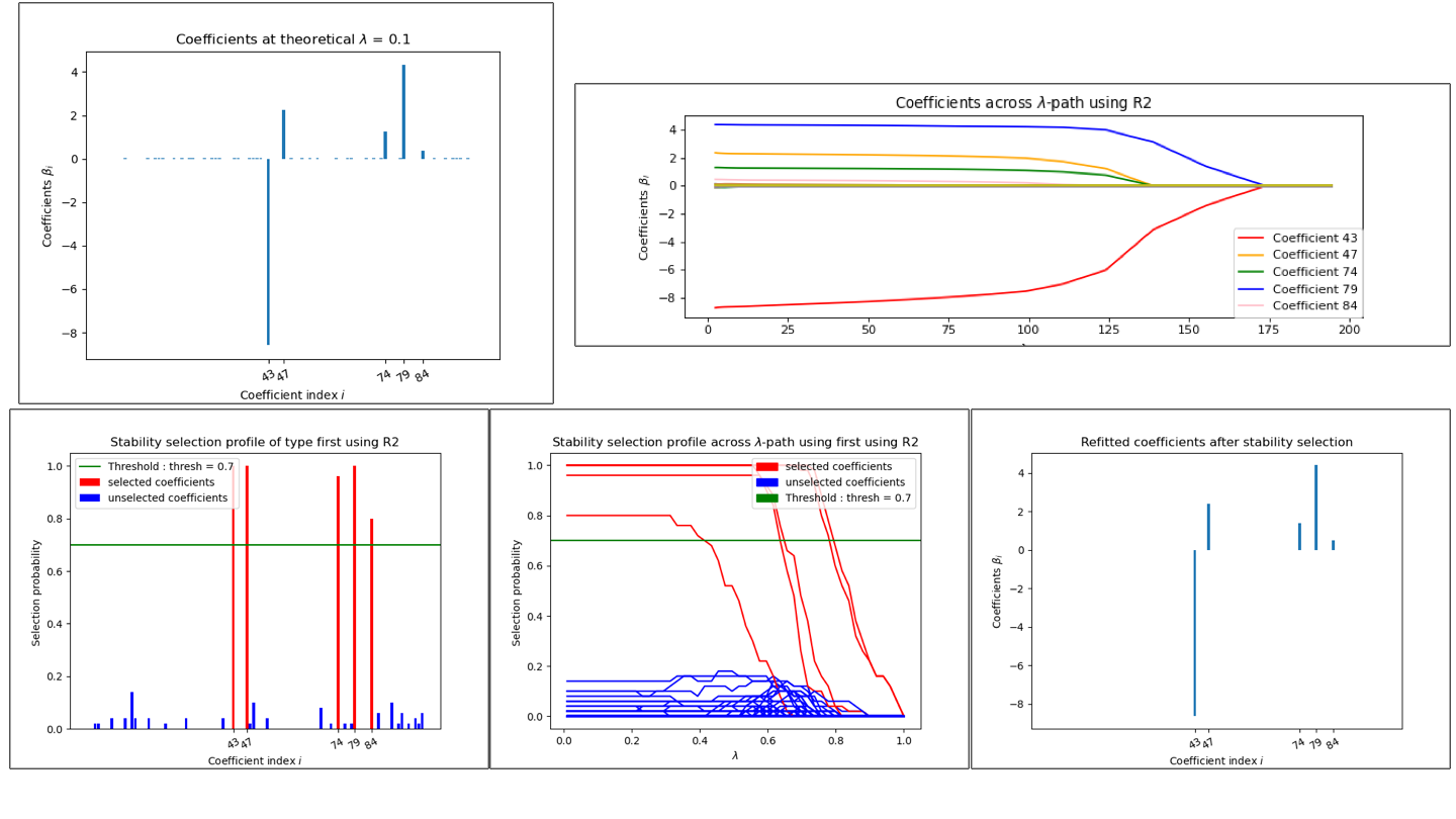
Figure 1: Visualizations after calling problem.solution

For this tuned example, the solutions at the fixed lambda and with stability selection recover the oracle solution. The solution vectors are stored in problem.solution and can be directly acccessed for each mode/model selection.

# Access to the estimated coefficient vector at a fixed lambda problem.solution.LAMfixed.beta

Note that the run time for this $d=100$-dimensional example for a single path computation is about 0.5 seconds on a standard Laptop.

Log-contrast regression on gut microbiome data

We next illustrate the application of c-lasso on the https://github.com/Leo-Simpson/c-lasso/tree/master/examples/COMBO_datahttps://doi.orgCOMBO microbiome dataset (Lin et al. 2014; Shi, Zhang, and Li 2016; Combettes and Müller 2020b). Here, the task is to predict the Body Mass Index (BMI) of $n=96$ participants from $d=45$ relative abundances of bacterial genera, and absolute calorie and fat intake measurements. The code snippet for this example is available in the https://github.com/Leo-Simpson/c-lasso/README.mdhttps://doi.orgREADME.md and the https://github.com/Leo-Simpson/c-lasso/blob/master/examples/example-notebook.ipynbhttps://doi.orgexample notebook.

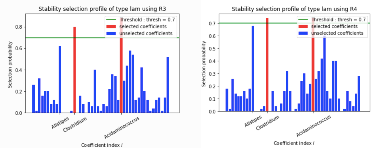
Figure 2: Stability selection profiles of problems R3/R4 on the COMBO data

Stability selection profiles using formulation R3 (left) and R4(right) on the COMBO dataset, reproducing Figure 5a in (Combettes and Müller 2020b).

Calling c-lasso in R

The c-lasso package also integrates with R via the R package https://rstudio.github.io/reticulate/https://doi.orgreticulate. We refer to reticulate’s manual for technical details about connecting python environments and R. A successful use case of c-lasso is available in the R package https://github.com/jacobbien/trachttps://doi.orgtrac (Bien et al. 2020), enabling tree-structured aggregation of predictors when features are rare.

The code snippet below shows how c-lasso is called in R to perform regression at a fixed $\lambda$ $\lambda=0.1\lambda_{\max}$. In R, X and C need to be of matrix type, and y of array type.

problem <- classo$classo_problem(X=X,C=C,y=y) problem$model_selection$LAMfixed <- TRUEproblem$model_selection$StabSel <- FALSEproblem$model_selection$LAMfixedparameters$rescaled_lam <- TRUEproblem$model_selection$LAMfixedparameters$lam <- 0.1problem$solve()# Extract coefficent vector with tidy-versebeta <- as.matrix(map_dfc(problem$solution$LAMfixed$beta, as.numeric))

References

Aitchion, J., and J. Bacon-Shone. 1984. “Log Contrast Models for Experiments with Mixtures.” Biometrika 71 (2): 323–30. doi:https://doi.org/10.1093/biomet/71.2.323https://doi.org10.1093/biomet/71.2.323.

Bien, Jacob, Xiaohan Yan, Léo Simpson, and Christian L Müller. 2020. “Tree-Aggregated Predictive Modeling of Microbiome Data.” bioRxiv. Cold Spring Harbor Laboratory. doi:https://doi.org/10.1101/2020.09.01.277632https://doi.org10.1101/2020.09.01.277632.

Briceño-Arias, Luis, and Sergio López Rivera. 2019. “A Projected Primal–Dual Method for Solving Constrained Monotone Inclusions.” Journal of Optimization Theory and Applications 180 (3): 907–24. doi:https://doi.org/10.1007/s10957-018-1430-2https://doi.org10.1007/s10957-018-1430-2.

Combettes, Patrick L., and Christian L. Müller. 2020a. “Perspective Maximum Likelihood-Type Estimation via Proximal Decomposition.” Electron. J. Statist. 14 (1). The Institute of Mathematical Statistics; the Bernoulli Society: 207–38. doi:https://doi.org/10.1214/19-EJS1662https://doi.org10.1214/19-EJS1662.

———. 2020b. “Regression Models for Compositional Data: General Log-Contrast Formulations, Proximal Optimization, and Microbiome Data Applications.” Statistics in Biosciences. doi:https://doi.org/10.1007/s12561-020-09283-2https://doi.org10.1007/s12561-020-09283-2.

Combettes, Patrick L., and Jean-Christophe Pesquet. 2012. “Primal-Dual Splitting Algorithm for Solving Inclusions with Mixtures of Composite, Lipschitzian, and Parallel-Sum Type Monotone Operators.” Set-Valued and Variational Analysis 20 (June): 307–20. doi:https://doi.org/10.1007/s11228-011-0191-yhttps://doi.org10.1007/s11228-011-0191-y.

Gaines, Brian R., Juhyun Kim, and Hua Zhou. 2018. “Algorithms for Fitting the Constrained Lasso.” Journal of Computational and Graphical Statistics 27 (4). Taylor & Francis: 861–71. doi:https://doi.org/10.1080/10618600.2018.1473777https://doi.org10.1080/10618600.2018.1473777.

Hastie, T., R. Tibshirani, and J.H. Friedman. 2009. The Elements of Statistical Learning: Data Mining, Inference, and Prediction. Springer Series in Statistics. Springer. https://books.google.fr/books?id=eBSgoAEACAAJ.

Huber, P. 1981. Robust statistics. John Wiley & Sons Inc.

James, Gareth M., Courtney Paulson, and Paat Rusmevichientong. 2020. “Penalized and Constrained Optimization: An Application to High-Dimensional Website Advertising.” Journal of the American Statistical Association 115 (529). Taylor & Francis: 107–22. doi:https://doi.org/10.1080/01621459.2019.1609970https://doi.org10.1080/01621459.2019.1609970.

Jeon, Jong-June, Yongdai Kim, Sungho Won, and Hosik Choi. 2020. “Primal path algorithm for compositional data analysis.” Computational Statistics & Data Analysis 148: 106958. doi:https://doi.org/https://doi.org/10.1016/j.csda.2020.106958https://doi.orghttps://doi.org/10.1016/j.csda.2020.106958.

Lee, Ching-Pei, and Chih-Jen Lin. 2013. “A Study on L2-Loss (Squared Hinge-Loss) Multiclass Svm.” Neural Computation 25 (March). doi:https://doi.org/10.1162/NECO_a_00434https://doi.org10.1162/NECO_a_00434.

Lin, Wei, Pixu Shi, Rui Feng, and Hongzhe Li. 2014. “Variable selection in regression with compositional covariates.” Biometrika 101 (4): 785–97. doi:https://doi.org/10.1093/biomet/asu031https://doi.org10.1093/biomet/asu031.

Meinshausen, Nicolai, and Peter Bühlmann. 2010. “Stability Selection.” Journal of the Royal Statistical Society: Series B (Statistical Methodology) 72 (4): 417–73. doi:https://doi.org/10.1111/j.1467-9868.2010.00740.xhttps://doi.org10.1111/j.1467-9868.2010.00740.x.

Mishra, Aditya, and Christian L. Müller. 2019. “Robust regression with compositional covariates.” http://arxiv.org/abs/1909.04990.

Rosset, Saharon, and Ji Zhu. 2007. “Piecewise linear regularized solution paths.” Annals of Statistics 35 (3): 1012–30. doi:https://doi.org/10.1214/009053606000001370https://doi.org10.1214/009053606000001370.

Shi, Pixu, Anru Zhang, and Hongzhe Li. 2016. “Regression analysis for microbiome compositional data.” Annals of Applied Statistics 10 (2): 1019–40. doi:https://doi.org/10.1214/16-AOAS928https://doi.org10.1214/16-AOAS928.