Stochastic Discontinuous Galerkin Methods with Low–Rank Solvers for Convection Diffusion Equations

Abstract

We investigate numerical behaviour of a convection diffusion equation with random coefficients by approximating statistical moments of the solution. Stochastic Galerkin approach, turning the original stochastic problem to a system of deterministic convection diffusion equations, is used to handle the stochastic domain in this study, whereas discontinuous Galerkin method is used to discretize spatial domain due to its local mass conservativity. A priori error estimates of the stationary problem and stability estimate of the unsteady model problem are derived in the energy norm. To address the curse of dimensionality of Stochastic Galerkin method, we take advantage of the low–rank Krylov subspace methods, which reduce both the storage requirements and the computational complexity by exploiting a Kronecker–product structure of system matrices. The efficiency of the proposed methodology is illustrated by numerical experiments on the benchmark problems.

1 Introduction

To simulate complex behaviors of physical systems, ones make predictions and hypotheses about certain outputs of interest with the help of simulation of mathematical models. However, due to the lack of knowledge or inherent variability in the model parameters, such real-problems formulated by mathematical models generally come with uncertainty concerning computed quantities; see, e.g., [38]. Therefore, the idea of uncertainty quantification, i.e., quantifying the effects of uncertainty on the result of a computation, has become a powerful tool for modeling physical phenomena in the last few years.

In order to solve PDEs with random coefficients, there exist three competing methods in the literature: the Monte Carlo method [17, 29], the stochastic collocation method [3, 45], and the stochastic Galerkin method [4, 22]. Although the Monte Carlo method is popular for its simplicity, natural parallelization, and broad applications, it features slow convergence. For the stochastic collocation methods, the crucial issue is how to construct the set of collocation points appropriately because the choice of the collocation points determines the efficiency of the method. In contrast to the Monte Carlo approach and the stochastic collocation method, the stochastic Galerkin method is a nonsampling approach, which transforms a PDE with random coefficients into a large system of coupled deterministic PDEs. As in the classic (deterministic) Galerkin method, the idea behind the stochastic Galerkin method is to seek a solution for the model equation such that the residue is orthogonal to the space of polynomials. An important feature of this technique is the separation of the spatial and stochastic variables, which allows a reuse of established numerical techniques.

In this paper, we mainly focus on the numerical investigation of a convection diffusion equation with random coefficients by using the stochastic Galerkin approach. Corresponding PDE can be considered as a basic model for transport phenomena in random media. For petroleum reservoir simulations or groundwater flow problems, permeability is desperately needed; however, it is hard to accurately measure permeability field in the earth due to the large area of oil reservoir and complicated earth structure. Hence, it is reasonable to model the permeability parameter as a random field, which corresponds to the solution of a convection diffusion equation; see, e.g., [20, 44]. In the literature, several stochastic finite element methods have been proposed and analysed, see, e.g., [4, 5, 13, 16, 18, 33, 46] and the references therein. However, there are a few work on the formulation and analysis of stochastic discontinuous Galerkin method; see, for instance [10, 47]. To the best of the authors’ knowledge, there exists any study on an analysis of stochastic discontinuous Galerkin methods with convection diffusion equations. With the present paper, we intend to fill this gap. Compared with the discontinuous Galerkin method, the finite difference method is not able to handle complex geometries, the finite volume method is not capable of achieving high–order accuracy, and the standard continuous finite element method lacks the ability of local mass conservation. Moreover, especially for convection dominated problems, DG methods produce stable concretization without the need for stabilization strategies and they allow for different orders of approximation to be used on different elements in a very straightforward manner [1, 37].

A major drawback of the stochastic Galerkin methods is the rapid increase of dimensionality, called as the curse of dimensionality. We address this issue by using low–rank Krylov subspace methods, which reduce both the storage requirements and the computational complexity by exploiting a Kronecker–product structure of system matrices, see, e.g., [6, 26, 40]. Similar approaches have been used to solve steady stochastic diffusion equations [12, 27, 34], unsteady stochastic diffusion equations [7], and stochastic Navier–Stokes equations [15, 28]. In the aforementioned studies, randomness is generally defined in the diffusion parameter however we here consider the randomness both in diffusion or convection parameters.

The rest of the paper is organized as follows: In the next section, we introduce our stationary model problem, that is, a convection diffusion equation with random coefficients, and provide an overview of its discretization, obtained by Karhunen–Loève (KL) expansion, stochastic Galerkin method, and discontinuous Galerkin method. In Section 3, we derive a priori error estimates for the stationary problem and stability estimates for the unsteady model problem in the energy norm. We discuss the implementation of low–rank iterative solvers in Section 4. As an extension of the concepts in Section 2, we proceed to Section 5 to introduce and analyze our strategy for the unsteady analogue of the steady–state model. Numerical results are given in Section 6 to show the efficiency of the proposed approach. Finally, we draw some conclusions and discussions in Section 7 based on the findings in the paper.

2 Stationary model problem with random coefficients

Let $\mathcal{D}\subset\mathbb{R}^{2}$ be a bounded open set with Lipschitz boundary $\partial\mathcal{D}$, and the triplet $(\Omega,\mathcal{F},\mathbb{P})$ denotes a complete probability space, where $\Omega$ is a sample space of events, $\mathcal{F}\subset 2^{\Omega}$ denotes a $\sigma$–algebra, and $\mathbb{P}:\mathcal{F}\rightarrow[0,1]$ is the associated probability measure. A generic random field $\eta$ on the probability space $(\Omega,\mathcal{F},\mathbb{P})$ is denoted by $\eta(x,\omega):\mathcal{D}\times\Omega\rightarrow\mathbb{R}$. For a fixed $x\in\mathcal{D}$, $\eta(x,\cdot)$ is a real–value square integrable random variable, i.e.,

$$\eta(x,\cdot)\in L^{2}(\Omega,\mathcal{F},\mathbb{P}):=\{X:\Omega\rightarrow\mathbb{R}\,:\;\int_{\Omega}|X(\omega)|^{2}\,d\mathbb{P}(\omega)<\infty\},$$

where $L^{2}(\Omega)=L^{2}(\Omega,\mathcal{F},\mathbb{P})$ is equipped with the norm $\left\langle{XY}\right\rangle=\left(\int_{\Omega}X\,Y\,d\mathbb{P}(\omega)\right)^{1/2}$. We denote the mean of $\eta(\mathbf{x},\omega)$ at a point $\mathbf{x}\in\mathcal{D}$ by $\overline{\eta}(\mathbf{x}):=\left\langle{\eta(x,\cdot)}\right\rangle$. Then, the covariance of $\eta$ at $\mathbf{x},\mathbf{y}\in\mathcal{D}$ is given by

$$\mathcal{C}_{\eta}(\mathbf{x},\mathbf{y}):=\left\langle{(\eta(\mathbf{x},\cdot)-\overline{\eta}(\mathbf{x}))(\eta(\mathbf{y},\cdot)-\overline{\eta}(\mathbf{y}))}\right\rangle.$$ (1)

If we set $\mathbf{x}=\mathbf{y}$ in (1), the variance $\mathcal{V}_{\eta}$ is obtained at $\mathbf{x}\in\mathcal{D}$. We also note that the standard derivation of $\eta$ is $\kappa=\sqrt{\mathcal{V}_{\eta}}$.

As a model problem, we first consider a stationary convection diffusion equation with random coefficients: find a random function $u:\overline{\mathcal{D}}\times\Omega\rightarrow\mathbb{R}$ such that $\mathbb{P}$-almost surely in $\Omega$

$$-\nabla\cdot(a(x,\omega)\nabla u(x,\omega))+\mathbf{b}(x,\omega)\cdot\nabla u(x,\omega) = f(x)\quad\hbox{ in}\;\;\mathcal{D}\times\Omega,$$ (2a)

$$u(x,\omega) = u_{d}(x)\quad\hbox{on}\;\;\partial\mathcal{D}\times\Omega,$$ (2b)

where $a:(\mathcal{D}\times\Omega)\rightarrow\mathbb{R}$ and $\mathbf{b}:(\mathcal{D}\times\Omega)\rightarrow\mathbb{R}^{2}$ are random diffusivity and velocity coefficients, respectively, which assumed to have continuous and bounded covariance functions. The functions $f(x)\in L^{2}(\mathcal{D})$ and $u_{d}(x)\in L^{2}(\mathcal{D})$ correspond to the deterministic source term and Dirichlet boundary condition, respectively. To show the regularity of the solution $u$, we need to make the following assumptions:

• The diffusivity coefficient $a(x,\omega)$ is $\mathbb{P}$–almost surely uniformly positive, that is, there exist constants $a_{\min},a_{\max}$ such that $0<a_{\min}\leq a_{\max}<\infty$, with

  $$a_{\min}\leq a(x,\omega)\leq a_{\max}\qquad\hbox{a. e.}\;\;\hbox{in }\mathcal{D}\times\Omega.$$ (3)

  The velocity coefficient $\mathbf{b}$ satisfies $\mathbf{b}\in\big{(}L^{\infty}(\overline{\mathcal{D}})\big{)}^{2}$ and $\nabla\cdot\mathbf{b}(x,\omega)=0$.

Under the assumptions on the coefficients provided above, the well–posedness of the model equation (2) follows from the classical Lax–Milgram lemma; see, e.g., [4, 32].

In the following, we introduce the well–known approach Karhunen–Lòeve expansion for the representation of the random coefficients, the solution representation via stochastic Galerkin method and symmetric interior penalty Galerkin method, and the resulting linear system.

2.1 Finite expansion of random fields

To solve the model problem (2) numerically, it is needed to reduce the stochastic process into a finite number of mutually uncorrelated, sometimes mutually independent, random variables. Therefore, we assume that the given coefficients $a(x,\omega)$ and $\mathbf{b}(x,\omega)$ can be approximated by a prescribed finite number of uncorrelated components $\xi_{i}(\omega),\;i=1,\ldots,N\in\mathbb{N}$, called as finite dimensional noise [4, 43]. Let $\Gamma_{i}=\xi_{i}(\Omega)\in\mathbb{R}$ be a bounded interval and $\rho_{i}\,:\,\Gamma_{i}\rightarrow[0,1]$ be the probability density functions of the random variables $\xi_{i}(\omega),\;i=1,\ldots,N\in\mathbb{N}$ with $\omega\in\Omega$. Then, the joint probability density function and the support of such probability density are denoted by $\rho(\xi),\;\xi\in\Gamma$ and $\Gamma=\prod\limits_{n=1}^{N}\Gamma_{n}$, respectively.

Following the Karhunen–Lòeve (KL) expansion [24, 31], a random field $\eta(\mathbf{x},\omega):\mathcal{D}\times\Omega\rightarrow\mathbb{R}$ with a continuous covariance function $\mathcal{C}_{\eta}(\mathbf{x},\mathbf{y})$ defined in (1) admits a proper orthogonal decomposition

$$\eta(\mathbf{x},\omega)=\overline{\eta}(\mathbf{x})+\kappa\sum\limits_{k=1}^{\infty}\sqrt{\lambda_{k}}\phi_{k}(\mathbf{x})\xi_{k}(\omega),$$ (4)

where $\xi:=\{\xi_{1},\xi_{2},\ldots\}$ are uncorrelated random variables. The pair $\{\lambda_{k},\phi_{k}\}$ is a set of the eigenvalues and eigenfunctions of the corresponding covariance operator $\mathcal{C}_{\eta}$. In order to obtain eigenpairs $\{\lambda_{k},\phi_{k}\}$, ones need to solve the following eigenvalue problem

$$\int_{\mathcal{D}}\mathcal{C}_{\eta}(\mathbf{x},\mathbf{y})\phi(\mathbf{y})\;d\mathbf{y}=\lambda_{i}\phi(\mathbf{x}).$$

It is noted that as long as the correlation is not zero, the eigenvalues $\{\lambda_{k}\}$ form a sequence of nonnegative real numbers decreasing to zero. We approximate $\eta(\mathbf{x},\omega)$ by truncating its KL expansion of the form

$$\eta(\mathbf{x},\omega)\approx\eta_{N}(\mathbf{x},\omega):=\overline{\eta}(\mathbf{x})+\kappa\sum\limits_{k=1}^{N}\sqrt{\lambda_{k}}\phi_{k}(\mathbf{x})\xi_{k}(\omega).$$ (5)

Here, the choice of the truncated number $N$ is usually based on the speed of decay on the eigenvalues since

$$\sum\limits_{i=1}^{\infty}\lambda_{i}=\int_{\mathcal{D}}\mathcal{V}_{\eta}(\mathbf{x})\,d\mathbf{x}.$$

The truncated KL expansion (5) is a finite representation of the random field $\eta(\mathbf{x},\omega)$ in the sense that the mean-square error of approximation is minimized; see, e.g., [2].

By the assumption based on finite dimensional noise and Doob–Dynkin lemma [35], we can replace the probability space $(\Omega,\mathcal{F},\mathbb{P})$ with $(\Gamma,\mathcal{B}(\Gamma),\rho(\xi)d\xi)$, where $\mathcal{B}(\Gamma)$ denotes Borel $\sigma$–algebra and $\rho(\xi)d\xi$ is the distribution measure of the vector $\xi$. Then, the solution corresponding to the stochastic PDE (2) admits exactly the same parametrization, that is, $u(\mathbf{x},\omega)=u(\mathbf{x},\xi_{1}(\omega),\xi_{2}(\omega),\ldots,\xi_{N}(\omega))$. Hence, we can state the tensor–product space $H^{k}(\mathcal{D})\otimes L^{2}(\Gamma)$, which is endowed with the norm

$$\|\eta\|_{H^{k}(\mathcal{D})\otimes L^{2}(\Gamma)}:=\left(\int_{\Gamma}\|\eta(\cdot,\xi)\|^{2}_{H^{k}(\mathcal{D})}\rho(\xi)\,d\xi\right)^{1/2}<\infty.$$

Further, the following isomorphism relation holds

$$H^{k}(\mathcal{D})\otimes L^{2}(\Gamma)\simeq L^{2}(H^{k}(\mathcal{D});\Gamma)\simeq H^{k}(\mathcal{D};L^{2}(\Gamma)).$$

Remark 2.1.

The covariance functions or eigenpairs can be computed explicitly for some random inputs, such as Gaussian or uniform processes with the exponential covariance function. However, they are usually not known a priori and therefore can be approximated numerically, such as collocation and Galerkin methods, see [32] for more details.

2.2 Stochastic Galerkin Method

The solution of the model problem (2), $u(x,\omega)\in L^{2}(\Omega,\mathcal{F},\mathbb{P})$, is represented by a generalized polynomial chaos (PC) approximation

$$u(x,\omega)=\sum_{i=0}^{\infty}u_{i}(x)\psi_{i}(\xi(\omega)),$$ (6)

where $u_{i}(x)$, the deterministic modes of the expansion, are given by

$$u_{i}(x)=\frac{\left\langle{u(x,\omega)\psi_{i}(\xi)}\right\rangle}{\left\langle{\psi_{i}^{2}(\xi)}\right\rangle},$$

$\xi$ is a finite–dimensional random vector, and $\psi_{i}$ are multivariate orthogonal polynomials having the following properties:

$$\left\langle{\psi_{0}(\xi)}\right\rangle=1,\qquad\left\langle{\psi_{i}(\xi)}\right\rangle=0,\quad i>0,\qquad\left\langle{\psi_{i}(\xi)\psi_{j}(\xi)}\right\rangle=\left\langle{\psi_{i}^{2}(\xi)}\right\rangle\delta_{ij}$$

with

$$\left\langle{\psi_{i}(\xi)}\right\rangle=\int_{\omega\in\Omega}\psi_{i}(\xi(\omega))\,d\mathbb{P}(\omega)=\int_{\xi\in\Gamma}\psi_{i}(\xi)\rho(\xi)\,d\xi,$$

where $\Gamma$ and $\rho$ are the support and probability density function of $\xi$, respectively. The orthogonal polynomials, i.e., $\psi_{i}$, are chosen according to the type of the distribution of random input, for instance, Hermite polynomials and Gaussian random variables, Legendre polynomials and uniform random variables, Laguerre polynomials and gamma random variables [25]. The probability density functions of random distributions are corresponding to the weight functions of some particular types of orthogonal polynomials.

The Cameron–Martin theorem [9] states that the series (6) converges in the Hilbert space $L^{2}(\Omega,\mathcal{F},\mathbb{P})$. Then, as done in the case of KL expansion (5), we truncate (6) as

$$u(x,\omega)\approx u_{P}(x,\omega)=\sum_{i=0}^{P-1}u_{i}(x)\psi_{i}(\xi(\omega)),$$ (7)

where the total number of PC basis is determined by the dimension $N$ of the random vector $\xi$ and the highest order $Q$ of the basis polynomials $\psi_{i}$

$$P=1+\sum\limits_{s=1}^{Q}\frac{1}{s!}\prod\limits_{j=0}^{s-1}(N+j)=\frac{(N+Q)!}{N!Q!}.$$

Then, the corresponding stochastic space is denoted by

$$\mathcal{Y}_{n}:=\hbox{span}\{\psi_{i}(\xi):\;i=0,1,\ldots,P-1\}\subset L^{2}(\Gamma).$$ (8)

We refer to [16, 36] and references therein for the construction of the stochastic space $\mathcal{Y}_{n}$.

Next, if we insert KL expansions (5) of the diffusion $a(x,\omega)$ and the convection $\mathbf{b}(x,\omega)$ coefficients, and the solution expression (7) into (2), we obtain

$$- \sum_{i=0}^{P-1}\nabla\cdot\Bigg{(}\Bigg{(}\overline{a}(x)+\kappa_{a}\sum_{k=1}^{N}\sqrt{\lambda_{k}^{a}}\phi_{k}^{a}(x)\xi_{k}\Bigg{)}\nabla u_{i}(x)\psi_{i}\Bigg{)}$$ (9)

$$\qquad+\sum_{i=0}^{P-1}\Bigg{(}\overline{\mathbf{b}}(x)+\kappa_{\mathbf{b}}\sum_{k=1}^{N}\sqrt{\lambda_{k}^{b}}\phi_{k}^{b}(x)\xi_{k}\Bigg{)}\cdot\nabla u_{i}(x)\psi_{i}=f(x).$$

By projecting (9) onto the space spanned by the PC basis functions, we obtain the following linear system, consisting of $P$ deterministic convection diffusion equations for $j=0,...,P-1$

$$-\sum_{i=0}^{P-1}\big{(}\nabla\cdot(a_{ij}\nabla u_{i}(x))+\mathbf{b}_{ij}\cdot\nabla u_{i}(x)\big{)}=\left\langle{\psi_{j}}\right\rangle f(x),$$ (10)

where

$$a_{ij} = \overline{a}(x)\left\langle{\psi_{i}^{2}(\xi)}\right\rangle\delta_{ij}+\kappa_{a}\sum_{k=1}^{N}\sqrt{\lambda_{k}^{a}}\phi_{k}^{a}(x)\left\langle{\xi_{k}\psi_{i}(\xi)\psi_{j}(\xi)}\right\rangle,$$

$$\mathbf{b}_{ij} = \overline{\mathbf{b}}(x)\left\langle{\psi_{i}^{2}(\xi)}\right\rangle\delta_{ij}+\kappa_{\mathbf{b}}\sum_{k=1}^{N}\sqrt{\lambda_{k}^{\mathbf{b}}}\phi_{k}^{\mathbf{b}}(x)\left\langle{\xi_{k}\psi_{i}(\xi)\psi_{j}(\xi)}\right\rangle.$$

Here, the quantity of interest is the statistical moments of the solution $u(x,\omega)$ in (2) rather than the solution $u(x,\omega)$. Once the modes $u_{i},\;i=0,1,\ldots,P-1$, have been computed, the statistical moments and the probability density of the solution can be easily deduced. For instance, the mean and the variance of the solution are

$$\left\langle{u(x,\xi)}\right\rangle=u_{0}(x),\qquad\mathcal{V}(u(x,\xi))=\sum\limits_{i=1}^{P-1}u_{i}^{2}(x)\left\langle{\psi_{i}^{2}(\xi)}\right\rangle,$$ (11)

respectively.

2.3 Symmetric interior penalty Galerkin method

Let $\{\mathcal{T}_{h}\}_{h}$ be a family of shape-regular simplicial triangulations of $\mathcal{D}$. Each mesh $\mathcal{T}_{h}$ consists of closed triangles such that $\overline{\mathcal{D}}=\bigcup_{K\in\mathcal{T}_{h}}\overline{K}$ holds. We assume that the mesh is regular in the following sense: for different triangles $K_{i},K_{j}\in\mathcal{T}_{h}$, $i\not=j$, the intersection $K_{i}\cap K_{j}$ is either empty or a vertex or an edge, i.e., hanging nodes are not allowed. The diameter of an element $K$ and the length of an edge $E$ are denoted by $h_{K}$ and $h_{E}$, respectively. Further, the maximum value of the element diameter is denoted by $h=\max\limits_{K\in\mathcal{T}_{h}}h_{K}$.

We split the set of all edges $\mathcal{E}_{h}$ into the set $\mathcal{E}^{0}_{h}$ of interior edges and the set $\mathcal{E}^{\partial}_{h}$ of boundary edges so that $\mathcal{E}_{h}=\mathcal{E}^{0}_{h}\cup\mathcal{E}^{\partial}_{h}$. Let $\mathbf{n}$ denote the unit outward normal to $\partial\mathcal{D}$. For a fixed realization $\omega$, the inflow and outflow parts of $\partial\mathcal{D}$ are denoted by $\partial\mathcal{D}^{-}$ and $\partial\mathcal{D}^{+}$, respectively,

$$\partial\mathcal{D}^{-}=\left\{{x\in\partial\mathcal{D}}\,:~{}{\mathbf{b}(x,\omega)\cdot\mathbf{n}(x)<0}\right\},\;\partial\mathcal{D}^{+}=\left\{{x\in\partial\mathcal{D}}\,:~{}{\mathbf{b}(x,\omega)\cdot\mathbf{n}(x)\geq 0}\right\}.$$

Similarly, the inflow and outflow boundaries of an element $K$ are defined by

$$\partial K^{-}=\left\{{x\in\partial K}\,:~{}{\mathbf{b}(x,\omega)\cdot\mathbf{n}_{K}(x)<0}\right\},\partial K^{+}=\left\{{x\in\partial K}\,:~{}{\mathbf{b}(x,\omega)\cdot\mathbf{n}_{K}(x)\geq 0}\right\},$$

where $\mathbf{n}_{K}$ is the unit normal vector on the boundary $\partial K$ of an element $K$.

Let the edge $E$ be a common edge for two elements $K$ and $K^{e}$. For a piecewise continuous scalar function $u$, there are two traces of $u$ along $E$, denoted by $u|_{E}$ from inside $K$ and $u^{e}|_{E}$ from inside $K^{e}$. The jump and average of $u$ across the edge $E$ are defined by:

$$\left[\!\left[u\right]\!\right] =u|_{E}\mathbf{n}_{K}+u^{e}|_{E}\mathbf{n}_{K^{e}},\quad\mbox{$\left\{\!\!\left\{u\right\}\!\!\right\}$}=\frac{1}{2}\big{(}u|_{E}+u^{e}|_{E}\big{)}.$$ (12)

Similarly, for a piecewise continuous vector field $\nabla u$, the jump and average across an edge $E$ are given by

$$\left[\!\left[\nabla u\right]\!\right] =\nabla u|_{E}\cdot\mathbf{n}_{K}+\nabla u^{e}|_{E}\cdot\mathbf{n}_{K^{e}},\quad\mbox{$\left\{\!\!\left\{\nabla u\right\}\!\!\right\}$}=\frac{1}{2}\big{(}\nabla u|_{E}+\nabla u^{e}|_{E}\big{)}.$$ (13)

For a boundary edge $E\in K\cap\partial\mathcal{D}$, we set $\mbox{$\left\{\!\!\left\{\nabla u\right\}\!\!\right\}$}=\nabla u$ and $\mbox{$\left[\!\left[u\right]\!\right]$}=u\mathbf{n}$, where $\mathbf{n}$ is the outward normal unit vector on $\partial\mathcal{D}$.

For an integer $\ell$ and $K\in\mathcal{T}_{h}$, let $\mathbb{P}^{\ell}(K)$ be the set of all polynomials on $K$ of degree at most $\ell$. Then, we define the discrete state and test spaces to be

$$V_{h} =\left\{{u\in L^{2}(\mathcal{D})}\,:~{}{u\mid_{K}\in\mathbb{P}^{\ell}(K)\quad\forall K\in\mathcal{T}_{h}}\right\}.$$ (14)

Note that since discontinuous Galerkin methods impose boundary conditions weakly, the space of discrete states and test functions are identical.

Following the standard discontinuous Galerkin structure in [1, 37], we define the following (bi)–linear forms for a finite dimensional vector $\xi$:

$$a_{h}(u,v,\xi) = \sum\limits_{K\in\mathcal{T}_{h}}\int\limits_{K}a(.,\xi)\nabla u\cdot\nabla v\,dx-\sum\limits_{E\in\mathcal{E}^{0}_{h}\cup\mathcal{E}_{h}^{\partial}}\int\limits_{E}\mbox{$\left\{\!\!\left\{a(.,\xi)\nabla u\right\}\!\!\right\}$}\mbox{$\left[\!\left[v\right]\!\right]$}\,ds$$

$$-\sum\limits_{E\in\mathcal{E}^{0}_{h}\cup\mathcal{E}_{h}^{\partial}}\int\limits_{E}\mbox{$\left\{\!\!\left\{a(.,\xi)\nabla v\right\}\!\!\right\}$}\mbox{$\left[\!\left[u\right]\!\right]$}\;ds+\sum\limits_{E\in\mathcal{E}^{0}_{h}\cup\mathcal{E}_{h}^{\partial}}\frac{\sigma}{h_{E}}\int\limits_{E}\mbox{$\left[\!\left[u\right]\!\right]$}\cdot\mbox{$\left[\!\left[v\right]\!\right]$}\,ds$$

$$+\sum\limits_{K\in\mathcal{T}_{h}}\int\limits_{K}\mathbf{b}(.,\xi)\cdot\nabla uv\;dx+\sum\limits_{K\in\mathcal{T}_{h}}\;\int\limits_{\partial K^{-}\backslash\partial\mathcal{D}}\mathbf{b}(.,\xi)\cdot\mathbf{n}_{E}(u^{e}-u)v\,ds$$

$$-\sum\limits_{K\in\mathcal{T}_{h}}\;\int\limits_{\partial K^{-}\cap\partial\mathcal{D}^{-}}\mathbf{b}(.,\xi)\cdot\mathbf{n}_{E}uv\,ds$$

and

$$l_{h}(v,\xi) = \sum\limits_{K\in\mathcal{T}_{h}}\int\limits_{K}fv\,dx+\sum\limits_{E\in\mathcal{E}_{h}^{\partial}}\frac{\sigma}{h_{E}}\int\limits_{E}u_{d}\mbox{$\left[\!\left[v\right]\!\right]$}\,ds-\sum\limits_{E\in\mathcal{E}_{h}^{\partial}}\int\limits_{E}u_{d}\mbox{$\left\{\!\!\left\{a(.,\xi)\nabla v\right\}\!\!\right\}$}\;ds$$

$$-\sum\limits_{K\in\mathcal{T}_{h}}\int\limits_{\partial K^{-}\cap\partial\mathcal{D}^{-}}\mathbf{b}(.,\xi)\cdot\mathbf{n}_{E}u_{d}v\,ds,$$

where the constant $\sigma>0$ is the interior penalty parameter. It has to be chosen sufficiently large independently of the mesh size to ensure the stability of the DG discretization.

Then, (bi)–linear forms of the stochastic discontinuous Galerkin (SDG) correspond to

$$a_{\xi}(u,v)=\int_{\Gamma}a_{h}(u,v,\xi)\rho(\xi)\,d\xi,\quad l_{\xi}(v)=\int_{\Gamma}l_{h}(v,\xi)\rho(\xi)\,d\xi.$$ (15)

Now, we define the associated energy norm on $\mathcal{D}\times\Gamma$ as

$$\lVert u\rVert_{\xi}=\Bigg{(}\int_{\Gamma}\lVert u(.,\xi)\rVert_{e}^{2}\rho(\xi)\,d\xi\Bigg{)}^{\frac{1}{2}},$$ (16)

where $\lVert u(.,\xi)\rVert_{e}$ is the energy norm on $\mathcal{D}$, given as

$$\lVert u(.,\xi)\rVert_{e} = \Bigg{(}\sum\limits_{K\in\mathcal{T}_{h}}\int\limits_{K}a(.,\xi)(\nabla u)^{2}\,dx+\sum\limits_{E\in\mathcal{E}^{0}_{h}\cup\mathcal{E}_{h}^{\partial}}\frac{\sigma}{h_{E}}\int\limits_{E}\mbox{$\left[\!\left[u\right]\!\right]$}^{2}\,ds$$

$$+\frac{1}{2}\sum\limits_{E\in\mathcal{E}_{h}^{\partial}}\int\limits_{E}\mathbf{b}(.,\xi)\cdot\mathbf{n}_{E}u^{2}ds+\frac{1}{2}\sum\limits_{E\in\mathcal{E}^{0}_{h}}\int\limits_{E}\mathbf{b}(.,\xi)\cdot\mathbf{n}_{E}(u^{e}-u)^{2}\,ds\Bigg{)}^{\frac{1}{2}}.$$

By standard arguments in deterministic case, ones can easily show the coercivity and continuity of $a_{\xi}(\cdot,\cdot)$ for $u,v\in V_{h}\otimes\mathcal{Y}_{n}$

$$a_{\xi}(u,u) \geq c_{cv}\,\lVert u\rVert_{\xi}^{2},$$ (17a)

$$a_{\xi}(u,v) \leq c_{ct}\,\lVert u\rVert_{\xi}\lVert v\rVert_{\xi},$$ (17b)

where the coercivity constant $c_{cv}$ depends on $a_{\min}$, whereas the continuity constant $c_{ct}$ depends on $a_{\max}$.

Thus, the SDG variational formulation of (2) is as follows: Find $u\in V_{h}\otimes\mathcal{Y}_{n}$ such that

$$a_{\xi}(u,v)=l_{\xi}(v),\qquad\forall v\in V_{h}\otimes\mathcal{Y}_{n}.$$ (18)

2.4 Linear System

After an application of the discretization techniques, one gets the following linear system:

$$\underbrace{\left(\sum_{i=0}^{N}\mathcal{G}_{i}\otimes\mathcal{K}_{i}\right)}_{\mathcal{A}}\,\mathbf{u}=\underbrace{\left(\sum_{i=0}^{N}\mathbf{g}_{i}\otimes\mathbf{f}_{i}\right)}_{\mathcal{F}},$$ (19)

where $\mathbf{u}=\left(u_{0},\ldots,u_{P-1}\right)^{T}\;\;\hbox{with}\;\;u_{i}\in\mathbb{R}^{N_{d}},\;\;i=0,1,\ldots,P-1$ and $N_{d}$ corresponds to the degree of freedom for the spatial discretization. The stiffness matrices $\mathcal{K}_{i}\in\mathbb{R}^{N_{d}\times N_{d}}$ and the right–hand side vectors $\mathbf{f}_{i}\in\mathbb{R}^{N_{d}}$ in (19) are given, respectively, by

$$\mathcal{K}_{0}(r,s) = \sum\limits_{K\in\mathcal{T}_{h}}\int\limits_{K}\left(\overline{a}\,\nabla\varphi_{r}\cdot\nabla\varphi_{s}+\overline{\mathbf{b}}\cdot\nabla\varphi_{r}\varphi_{s}\right)\,dx$$

$$-\sum\limits_{E\in\mathcal{E}^{0}_{h}\cup\mathcal{E}_{h}^{\partial}}\int\limits_{E}\big{(}\mbox{$\left\{\!\!\left\{\overline{a}\,\nabla\varphi_{r}\right\}\!\!\right\}$}\mbox{$\left[\!\left[\varphi_{s}\right]\!\right]$}+\mbox{$\left\{\!\!\left\{\overline{a}\,\nabla\varphi_{s}\right\}\!\!\right\}$}\mbox{$\left[\!\left[\varphi_{r}\right]\!\right]$}\big{)}\,ds$$

$$+\sum\limits_{E\in\mathcal{E}^{0}_{h}\cup\mathcal{E}_{h}^{\partial}}\frac{\sigma}{h_{E}}\int\limits_{E}\mbox{$\left[\!\left[\varphi_{r}\right]\!\right]$}\cdot\mbox{$\left[\!\left[\varphi_{s}\right]\!\right]$}\,ds+\sum\limits_{K\in\mathcal{T}_{h}}\;\int\limits_{\partial K^{-}\backslash\partial\mathcal{D}}\overline{\mathbf{b}}\cdot\mathbf{n}_{E}(\varphi_{r}^{e}-\varphi_{r})\varphi_{s}\,ds$$

$$-\sum\limits_{K\in\mathcal{T}_{h}}\;\int\limits_{\partial K^{-}\cap\partial\mathcal{D}^{-}}\overline{\mathbf{b}}\cdot\mathbf{n}_{E}\varphi_{r}\varphi_{s}\,ds,$$

$$\mathcal{K}_{i}(r,s) = \sum\limits_{K\in\mathcal{T}_{h}}\int\limits_{K}\left(\Big{(}\kappa_{a}\sqrt{\lambda_{i}^{a}}\phi_{i}^{a}\Big{)}\nabla\varphi_{r}\cdot\nabla\varphi_{s}+\Big{(}\kappa_{\mathbf{b}}\sqrt{\lambda_{i}^{\mathbf{b}}}\phi_{i}^{\mathbf{b}}\Big{)}\cdot\nabla\varphi_{r}\varphi_{s}\right)\,dx$$

$$-\sum\limits_{E\in\mathcal{E}^{0}_{h}\cup\mathcal{E}_{h}^{\partial}}\int\limits_{E}\left(\mbox{$\left\{\!\!\left\{\Big{(}\kappa_{a}\sqrt{\lambda_{i}^{a}}\phi_{i}^{a}\Big{)}\nabla\varphi_{r}\right\}\!\!\right\}$}\mbox{$\left[\!\left[\varphi_{s}\right]\!\right]$}+\mbox{$\left\{\!\!\left\{\Big{(}\kappa_{a}\sqrt{\lambda_{i}^{a}}\phi_{i}^{a}\Big{)}\nabla\varphi_{s}\right\}\!\!\right\}$}\mbox{$\left[\!\left[\varphi_{r}\right]\!\right]$}\right)\,ds$$

$$+\sum\limits_{E\in\mathcal{E}^{0}_{h}\cup\mathcal{E}_{h}^{\partial}}\frac{\sigma}{h_{E}}\int\limits_{E}\mbox{$\left[\!\left[\varphi_{r}\right]\!\right]$}\cdot\mbox{$\left[\!\left[\varphi_{s}\right]\!\right]$}\,ds$$

$$+\sum\limits_{K\in\mathcal{T}_{h}}\int\limits_{\partial K^{-}\backslash\partial\mathcal{D}}\Big{(}\kappa_{\mathbf{b}}\sqrt{\lambda_{i}^{\mathbf{b}}}\phi_{i}^{\mathbf{b}}\Big{)}\cdot\mathbf{n}_{E}(\varphi_{r}^{e}-\varphi_{r})\varphi_{s}\,ds$$

$$-\sum\limits_{T\in\mathcal{T}_{h}}\int\limits_{\partial K^{-}\cap\partial\mathcal{D}^{-}}\Big{(}\kappa_{\mathbf{b}}\sqrt{\lambda_{i}^{\mathbf{b}}}\phi_{i}^{\mathbf{b}}\Big{)}\cdot\mathbf{n}_{E}\varphi_{r}\varphi_{s}\,ds,$$

$$f_{0}(s) = \sum\limits_{K\in\mathcal{T}_{h}}\int\limits_{K}f\varphi_{s}\;dx+\sum\limits_{E\in\mathcal{E}_{h}^{\partial}}\frac{\sigma}{h_{E}}\int\limits_{E}u_{d}\mbox{$\left[\!\left[\varphi_{s}\right]\!\right]$}\;ds-\sum\limits_{E\in\mathcal{E}_{h}^{\partial}}\int\limits_{E}u_{d}\mbox{$\left\{\!\!\left\{\overline{a}\nabla\varphi_{s}\right\}\!\!\right\}$}\;ds$$

$$-\sum\limits_{K\in\mathcal{T}_{h}}\int\limits_{\partial K^{-}\cap\partial\mathcal{D}^{-}}\overline{\mathbf{b}}\cdot\mathbf{n}_{E}u_{d}\varphi_{s}\;ds,$$

$$f_{i}(s) = \sum\limits_{E\in\mathcal{E}_{h}^{\partial}}\frac{\sigma}{h_{E}}\int\limits_{E}u_{d}\mbox{$\left[\!\left[\varphi_{s}\right]\!\right]$}\;ds-\sum\limits_{E\in\mathcal{E}_{h}^{\partial}}\int\limits_{E}u_{d}\mbox{$\left\{\!\!\left\{\Big{(}\kappa_{a}\sqrt{\lambda_{i}^{a}}\phi_{i}^{a}\Big{)}\nabla\varphi_{s}\right\}\!\!\right\}$}\;ds\;$$

$$-\sum\limits_{K\in\mathcal{T}_{h}}\;\int\limits_{\partial K^{-}\cap\partial\mathcal{D}^{-}}\Big{(}\kappa_{\mathbf{b}}\sqrt{\lambda_{i}^{\mathbf{b}}}\phi_{i}^{\mathbf{b}}\Big{)}\cdot\mathbf{n}_{E}u_{d}\varphi_{s}\;ds,$$

where $\{\varphi_{i}(x)\}$ is the set of basis functions for the spatial discretization, i.e., $V_{h}=\hbox{span}\{\varphi_{i}(x)\}$.

For $i=0,\ldots,N$ the stochastic matrices $\mathcal{G}_{i}\in\mathbb{R}^{P\times P}$ in (19) are given by

$$\mathcal{G}_{0}(r,s)=\left\langle{\psi_{r}\psi_{s}}\right\rangle,\qquad\mathcal{G}_{i}(r,s)=\left\langle{\xi_{i}\psi_{r}\psi_{s}}\right\rangle,$$ (20)

whereas the stochastic vectors $\mathbf{g}_{i}\in\mathbb{R}^{P}$ in (19) are defined as

$$\mathbf{g}_{0}(r)=\left\langle{\psi_{r}}\right\rangle,\qquad\mathbf{g}_{i}(r)=\left\langle{\xi_{i}\psi_{r}}\right\rangle.$$ (21)

In (20) each stochastic basis function $\psi_{i}(\xi)$ is corresponding to a product of $N$ univariate orthogonal polynomials, i.e., $\psi_{i}(\xi)=\psi_{i_{1}}(\xi)\psi_{i_{2}}(\xi)\ldots\psi_{i_{N}}(\xi),$ where the multi–index $i$ is defined by $i=(i_{1},i_{2},\ldots,i_{N})$ with $\sum\limits_{s=1}^{N}i_{s}\leq Q$. In this paper, Legendre polynomials are chosen as stochastic basis functions because the underlying random variables have a uniform distribution.

Now, suppose we employ Legendre polynomials in uniform random variables on $(-\sqrt{3},\sqrt{3})$. Then, recalling the following three–term recurrence for the Legendre polynomials

$$\psi_{k+1}(x)=\frac{\sqrt{2k+1}\sqrt{2k+3}}{(k+1)\sqrt{3}}x\psi_{k}(x)-\dfrac{k\sqrt{2k+3}}{(k+1)\sqrt{2k-1}}\psi_{k-1}\;\hbox{with}\;\psi_{0}=1,\;\psi_{-1}=0,$$

we obtain

$$\mathcal{G}_{0}(i,j) = \prod_{s=1}^{N}\big{\langle}{\psi_{i_{s}}^{2}(\xi_{s})}\big{\rangle}\delta_{i_{s}j_{s}}=\prod_{s=1}^{N}\delta_{i_{s}j_{s}}=\begin{cases}1,&\mbox{if }i=j,\\ 0,&\mbox{otherwise}\end{cases}$$

and for $k=1:N$

$$\mathcal{G}_{k}(i,j) = \int_{\Gamma}\xi_{k}\psi_{i}(\vec{\xi})\psi_{j}(\vec{\xi})\rho(\vec{\xi})\;d\vec{\xi}$$

$$= \int_{-\sqrt{3}}^{\sqrt{3}}\cdots\int_{-\sqrt{3}}^{\sqrt{3}}\xi_{k}\psi_{i}(\vec{\xi})\psi_{j}(\vec{\xi})\rho(\vec{\xi})\;d\vec{\xi}$$

$$= \Bigg{(}\prod_{s=1,s\neq k}^{N}\left\langle{\psi_{i_{s}}(\xi_{s})\psi_{j_{s}}(\xi_{s})}\right\rangle\Bigg{)}\left\langle{\xi_{k}\psi_{i_{k}}(\xi_{k})\psi_{j_{k}}(\xi_{k})}\right\rangle$$

$$= \Bigg{(}\prod_{s=1,s\neq k}^{N}\left\langle{\psi_{i_{s}}(\xi_{s})\psi_{j_{s}}(\xi_{s})}\right\rangle\Bigg{)}$$

$$\;\,\times\left(\dfrac{(i_{k}+1)\sqrt{3}}{\sqrt{(2i_{k}+1)(2i_{k}+3)}}\left\langle{\psi_{i_{k}+1}\psi_{j_{k}}}\right\rangle+\dfrac{i_{k}\sqrt{3}}{\sqrt{(2i_{k}+1)(2i_{k}-1)}}\left\langle{\psi_{i_{k}-1}\psi_{j_{k}}}\right\rangle\right)$$

$$= \begin{cases}\Bigg{(}\prod\limits_{s=1,s\neq k}^{N}\delta_{i_{s}j_{s}}\Bigg{)}\dfrac{(i_{k}+1)\sqrt{3}}{\sqrt{(2i_{k}+1)(2i_{k}+3)}},&\mbox{if }i_{k}+1=j_{k},\\ \Bigg{(}\prod\limits_{s=1,s\neq k}^{N}\delta_{i_{s}j_{s}}\Bigg{)}\dfrac{i_{k}\sqrt{3}}{\sqrt{(2i_{k}+1)(2i_{k}-1)}},&\mbox{if }i_{k}-1=j_{k},\\ 0,&\mbox{otherwise}\end{cases}$$

$$= \begin{cases}\dfrac{(i_{k}+1)\sqrt{3}}{\sqrt{(2i_{k}+1)(2i_{k}+3)}},&\mbox{if }i_{k}+1=j_{k}\;\hbox{and}\;i_{s}=j_{s},\;s=\{1:N\}\setminus\{k\},\\ \dfrac{i_{k}\sqrt{3}}{\sqrt{(2i_{k}+1)(2i_{k}-1)}},&\mbox{if }i_{k}-1=j_{k}\;\hbox{and}\;i_{s}=j_{s},\;s=\{1:N\}\setminus\{k\},\\ 0,&\mbox{otherwise}.\end{cases}$$

Hence, $\mathcal{G}_{0}$ is a identity matrix, whereas $\mathcal{G}_{k},\;k>0$, contains at most two nonzero entries per row; see, e.g., [16, 36]. On the other hand, $\textbf{g}_{i}$ is the first column of $\mathcal{G}_{i},\;i=0,1,\ldots,N$.

3 Error estimates

In this section, we present a priori error estimates for stationary convection diffusion equations with random coefficients, discretized by stochastic discontinuous Galerkin method.

Let a partition of the support of probability density in finite dimensional space, i.e., $\Gamma=\prod\limits_{n=1}^{N}\Gamma_{n}$ consists of a finite number of disjoint $\mathbf{R}^{N}$–boxes, $\gamma=\prod\limits_{n=1}^{N}(r_{n}^{\gamma},s_{n}^{\gamma})$, with $(r_{n}^{\gamma},s_{n}^{\gamma})\subset\Gamma_{n}$ for $n=1,\ldots,N$. The mesh size $k_{n}$ is defined by $k_{n}=\max\limits_{\gamma}|s_{n}^{\gamma}-r_{n}^{\gamma}|$ for $1\leq n\leq N$. For the multi–index $q=(q_{1},\ldots,q_{N})$, the (discontinuous) finite element approximation space with degree at most $q_{n}$ on each direction $\xi_{n}$ is denoted by $\mathcal{Y}_{k}^{q}\subset L^{2}(\Gamma)$. Then, for $v\in H^{q+1}(\Gamma),\varphi\in\mathcal{Y}_{k}^{q}$, we have the following estimate, see, e.g., [4]

$$\min\limits_{\varphi\in\mathcal{Y}_{k}^{q}}\|v-\varphi\|_{L^{2}(\Gamma)}\leq\sum_{n=1}^{N}\bigg{(}\frac{k_{n}}{2}\bigg{)}^{q_{n}+1}\dfrac{\lVert\partial^{q_{n}+1}_{\xi_{n}}v\rVert_{L^{2}(\Gamma)}}{(q_{n}+1)!}.$$ (22)

To later use, we introduce the $L^{2}$–projection operator $\Pi_{n}:L^{2}(\Gamma)\rightarrow\mathcal{Y}_{k}^{q}$ by

$$(\Pi_{n}(\xi)-\xi,\zeta)_{L^{2}(\Gamma)}=0\qquad\quad\forall\zeta\in\mathcal{Y}_{k}^{q},\qquad\forall\xi\in L^{2}(\Gamma),$$ (23)

and the $H^{1}$–projection operator $\mathcal{R}_{h}:H^{1}(\mathcal{D})\rightarrow V_{h}\cap H^{1}(\mathcal{D})$ by

$$(\mathcal{R}_{h}(\nu)-\nu,\chi)_{L^{2}(\mathcal{D})} = 0\qquad\quad\forall\chi\in V_{h},\qquad\forall\nu\in H^{1}(\mathcal{D}),$$ (24a)

$$(\nabla(\mathcal{R}_{h}(\nu)-\nu),\nabla\chi)_{L^{2}(\mathcal{D})} = 0\qquad\quad\forall\chi\in V_{h},\qquad\forall\nu\in H^{1}(\mathcal{D}).$$ (24b)

Next, we state the well–known trace and inverse inequalities, which are needed frequently in the rest of the paper.

• For positive constant $c_{tr}$ independent of $K\in\mathcal{T}_{h}$ and $h$, the trace inequality is given as follow (see, e.g., [37, Section 2.1]):

  $$\lVert v\rVert_{E}^{2} \leq c_{tr}\bigg{(}\lVert v\rVert_{L^{2}(K)}^{2}+h_{K}\lvert v\rvert_{H^{1}(K)}^{2}\bigg{)}\quad v\in H^{1}(K),$$ (25a)

  $$\lVert\nabla v\cdot\mathbf{n_{E}}\rVert_{E}^{2} \leq c_{tr}\bigg{(}\lvert v\rvert_{H^{1}(K)}^{2}+h_{K}\lvert v\rvert_{H^{2}(K)}^{2}\bigg{)}\quad\;\,v\in H^{2}(K).$$ (25b)

• For positive constant $c_{inv}$ independent of $K\in\mathcal{T}_{h}$ and $h$, the inverse inequality is given as follows (see, e.g., [8, Section 4.5]):

  $$|v|_{j,K} \leq c_{inv}\,h^{i-j}|v|_{i,K}\qquad\quad\forall v\in V_{h},\qquad\;0\leq i\leq j\leq 2.$$ (26)

Lastly, we give discontinuous Galerkin approximation estimate for all $v\in H^{2}(K)$ for $K\in\mathcal{T}_{h}$.

Theorem 3.1.

([37, Theorem 2.6]) Assume that $v\in H^{2}(K)$ for $K\in\mathcal{T}_{h}$ and $\widetilde{v}\in\mathbb{P}^{\ell}$. Then, there exists a constant $C$ independent of $v$ and $h$ such that

$$\lVert v-\widetilde{v}\rVert_{H^{q}(K)}\leq C\,h^{\min(\ell+1,2)-q}\lvert v\rvert_{H^{2}(K)}\qquad 0\leq q\leq 2.$$ (27)

Let $\widetilde{u}\in V_{h}\otimes\mathcal{Y}_{k}^{q}$ is an approximation of the solution $u$. We derive an approximation for the tensor product $V_{h}\otimes\mathcal{Y}_{k}^{q}$, which is a direct application of the results for $V_{h}$ and $\mathcal{Y}_{k}^{q}$ as done in [4, 30].

Theorem 3.2.

Assume that $v\in L^{2}(H^{2}(\mathcal{D});\Gamma)\cap H^{q+1}(H^{1}(\mathcal{D});\Gamma)$ and $\widetilde{v}\in V_{h}\otimes\mathcal{Y}_{k}^{q}$. Then, we have

$$\lVert\nabla(v-\widetilde{v})\rVert_{L^{2}(L^{2}(\mathcal{D});\Gamma)} \leq Ch^{\min(\ell+1,2)-1}\lVert v\rVert_{L^{2}(H^{2}(\mathcal{D});\Gamma)}$$ (28a)

$$+\sum_{n=1}^{N}\bigg{(}\frac{k_{n}}{2}\bigg{)}^{q_{n}+1}\dfrac{\lVert\partial^{q_{n}+1}_{\xi_{n}}v\rVert_{L^{2}(H^{1}(\mathcal{D});\Gamma)}}{(q_{n}+1)!},$$

$$\lVert\nabla^{2}(v-\widetilde{v})\rVert_{L^{2}(L^{2}(\mathcal{D});\Gamma)} \leq Ch^{\min(\ell+1,2)-2}\lVert v\rVert_{L^{2}(H^{2}(\mathcal{D});\Gamma)}$$ (28b)

$$+Ch^{-1}\sum_{n=1}^{N}\bigg{(}\frac{k_{n}}{2}\bigg{)}^{q_{n}+1}\dfrac{\lVert\partial^{q_{n}+1}_{\xi_{n}}v\rVert_{L^{2}(H^{1}(\mathcal{D});\Gamma)}}{(q_{n}+1)!},$$

where the constant $C$ independent of $v$, $h$, and $k_{n}$.

Proof.

We refer to A for the proof of Theorem 3.2. ∎

The next step is to use Theorem 3.2 together with the approximation estimate (27) to derive an upper bound for the error in the energy norm.

Theorem 3.3.

Assume $u\in L^{2}(H^{2}(\mathcal{D});\Gamma)\cap H^{q+1}(H^{1}(\mathcal{D});\Gamma)$ and $u_{h}\in V_{h}\otimes\mathcal{Y}_{k}^{q}$. Then, there is a constant $C$ independent of $u,h$, and $k_{n}$ such that

$$\lVert u-u_{h}\rVert_{\xi} \leq C\left(h^{\min(\ell+1,2)-1}\lVert u\rVert_{L^{2}(H^{2}(\mathcal{D});\Gamma)}\right.$$ (29)

$$\left.+\sum_{n=1}^{N}\bigg{(}\frac{k_{n}}{2}\bigg{)}^{q_{n}+1}\dfrac{\lVert\partial^{q_{n}+1}_{\xi_{n}}u\rVert_{L^{2}(H^{1}(\mathcal{D});\Gamma)}}{(q_{n}+1)!}\right).$$

Proof.

We refer to B for the proof of Theorem 3.3. ∎

In practical implementations such as transport phenomena in random media, the length $N$ of the random vector $\xi$ can be large, especially for the small correlation length in the covariance function of the random input. This increases the value of multivariate stochastic basis polynomials $P$ quite fast, called as the curse of dimensionality. In the following section, we break the curse of dimensionality by using low–rank approximation, which reduces both the storage requirements and the computational complexity by exploiting a Kronecker–product structure of system matrices defined in (19).

4 Low–rank approximation

In this section, we develop efficient Krylov subspace solvers with suitable preconditioners where the solution is approximated using a low–rank representation in order to reduce memory requirements and computational effort. Basic operations associated with the low-rank format are much cheaper, and as Krylov subspace method converges, it constructs a sequence of low–rank approximations to the solution of the system.

We begin with the basic notation related to Kronecker products and low-rank approach. Let $\mathbf{u}=[u_{1}^{T},\ldots,u_{P}^{T}]^{T}\in\mathbb{R}^{N_{d}P}$ with each $u_{i}$ of length $N_{d}$ and $\mathbf{U}=[u_{1},\ldots,u_{P}]\in\mathbb{R}^{N_{d}\times P}$ where $N_{d}$ and $P$ are the degrees of freedom for the spatial discretization and the total degree of the multivariate stochastic basis polynomials, respectively. Then, we define isomorphic mappings between $\mathbb{R}^{N_{d}P}$ and $\mathbb{R}^{N_{d}\times P}$ as following

$$\texttt{vec}:\mathbb{R}^{N_{d}\times P}\rightarrow\mathbb{R}^{N_{d}P},\qquad\texttt{mat}:\mathbb{R}^{N_{d}P}\rightarrow\mathbb{R}^{N_{d}\times P}$$

determined by the operators vec($\cdot$) and mat($\cdot$), respectively. The matrix inner product is defined by $\left\langle{U,V}\right\rangle_{F}=\text{trace}(U^{T}V)$ so that the induced norm is $\|U\|_{F}=\sqrt{\left\langle{U,V}\right\rangle_{F}}$. For the sake of simplicity, we will omit the subscript in $\|\cdot\|_{F}$ and write only $\|\cdot\|$. Further, we have the following properties, see, e.g., [26]:

$$\texttt{vec}(A\mathbf{U}B)=(B^{T}\otimes A)\texttt{vec}(\mathbf{U}),\qquad(A\otimes B)(C\otimes D)=AC\otimes BD.$$

Now, we can interpret the system (19) as $\mathbf{\mathcal{A}}(U)=\mathcal{F}$ for the matrix $U\in\mathbb{R}^{N_{d}\times P}$ with $\mathbf{u}=\text{vec}(\mathbf{U})$, where $\mathbf{\mathcal{A}}(\mathbf{U})$ is defined as the linear operator satisfying $\text{vec}(\mathbf{\mathcal{A}}(\mathbf{U}))=\mathbf{\mathcal{A}}\text{vec}(\mathbf{U})$. Assuming low–rank decomposition of $\mathbf{U}=WV^{T}$ with

$$W=[w_{1},\ldots,w_{k}]\in\mathbb{R}^{N_{d}\times r},\quad V=[v_{1},\ldots,v_{k}]\in\mathbb{R}^{P\times r},\quad r\ll N_{d},P$$

and

$$\texttt{vec}(\mathbf{U})=\texttt{vec}\Bigg{(}\sum_{i=1}^{r}w_{i}v_{i}^{T}\Bigg{)}=\sum_{i=1}^{r}v_{i}\otimes w_{i},$$

we have

$$\mathbf{\mathcal{A}}\texttt{vec}(\mathbf{U}) = \Bigg{(}\sum_{k=0}^{N}\mathcal{G}_{k}\otimes\mathcal{K}_{k}\Bigg{)}\Bigg{(}\sum_{i=1}^{r}v_{i}\otimes w_{i}\Bigg{)}$$

$$= \sum_{k=0}^{N}\sum_{i=1}^{r}(\mathcal{G}_{k}v_{i})\otimes(\mathcal{K}_{k}w_{i})\in\mathbb{R}^{N_{d}P}.$$

This implies

$$\mathbf{\mathcal{A}}(\mathbf{U}):=\texttt{mat}(\mathbf{\mathcal{A}}\texttt{vec}(\mathbf{U}))\in\mathbb{R}^{N_{d}\times P}.$$

Algorithm 1 Low–rank preconditioned BiCGstab (LRPBiCGstab)

Input: Matrix functions $\mathcal{A},\mathcal{P}:\mathbb{R}^{N_{d}\times P}\rightarrow\mathbb{R}^{N_{d}\times P}$, right–hand side $\mathcal{F}$ in low–rank format. Truncation operator $\mathcal{T}$ w.r.t. given tolerance $\epsilon_{trunc}$.
     Output: Matrix $\mathbf{U}\in\mathbb{R}^{N_{d}\times P}$ satisfying $\|\mathcal{A}(\mathbf{U})-\mathcal{F}\|\leq\epsilon_{tol}$.

1: $\mathbf{U}_{0}=0$, $R_{0}=\mathcal{F}$, $\widetilde{R}=\mathcal{F}$, $\rho_{0}=\langle\widetilde{R},R_{0}\rangle$, $S_{0}=R_{0}$, $\widetilde{S}_{0}=\mathcal{P}^{-1}(S_{0})$, $V_{0}=\mathcal{A}(\widetilde{S}_{0})$, $k=0$

2: while $\lVert R_{k}\rVert>\epsilon_{tol}$ do

3:    $\omega_{k}=\langle\widetilde{R},R_{k}\rangle/\langle\widetilde{R},V_{k}\rangle$

4:    $Z_{k}=R_{k}-\omega_{k}V_{k}$, $Z_{k}\leftarrow\mathcal{T}(Z_{k})$

5:    $\widetilde{Z}_{k}=\mathcal{P}^{-1}(Z_{k})$, $\widetilde{Z}_{k}\leftarrow\mathcal{T}(\widetilde{Z}_{k})$

6:    $T_{k}=\mathcal{A}(\widetilde{Z}_{k})$, $T_{k}\leftarrow\mathcal{T}(T_{k})$

7:    if $\lVert Z_{k}\rVert\leq\epsilon_{tol}$ then

8:       $\mathbf{U}=\mathbf{U}_{k}+\omega_{k}\widetilde{S}_{k}$

9:       return  

10:    end if

11:    $\xi_{k}=\langle T_{k},Z_{k}\rangle/\langle T_{k},T_{k}\rangle$

12:    $\mathbf{U}_{k+1}=\mathbf{U}_{k}+\omega_{k}\widetilde{S}_{k}+\xi_{k}\widetilde{Z}_{k}$, $\mathbf{U}_{k+1}\leftarrow\mathcal{T}(\mathbf{U}_{k+1}^{n})$

13:    $R_{k+1}=\mathcal{F}-\mathcal{A}(\mathbf{U}_{k+1})$, $R_{k+1}\leftarrow\mathcal{T}(R_{k+1})$

14:    if $\lVert R_{k+1}\rVert\leq\epsilon_{tol}$ then

15:       $\mathbf{U}=\mathbf{U}_{k+1}$

16:       return  

17:    end if

18:    $\rho_{k+1}=\langle\widetilde{R},R_{k+1}\rangle$

19:    $\beta_{k}=\frac{\rho_{k+1}}{\rho_{k}}\frac{\omega_{k}}{\xi_{k}}$

20:    $S_{k+1}=R_{k+1}+\beta_{k}(S_{k}-\xi_{k}V_{k})$, $S_{k+1}\leftarrow\mathcal{T}(S_{k+1})$

21:    $\widetilde{S}_{k+1}=\mathcal{P}^{-1}(S_{k+1})$, $\widetilde{S}_{k+1}\leftarrow\mathcal{T}(\widetilde{S}_{k+1})$

22:    $V_{k+1}=\mathcal{A}(\widetilde{S}_{k+1})$, $V_{k+1}\leftarrow\mathcal{T}(V_{k+1})$

23:    $k=k+1$

24: end while

It is noted that in this study, we do not discuss the existence of the low–rank approximation. We refer to [7, 19] and references therein.

We here apply a variant of Krylov subspace solvers, namely, conjugate gradient (CG) method [23], bi–conjugate gradient stabilized (BiCGstab) [42], quasi–minimal residual variant of the bi–conjugate gradient stabilized (QMRCGstab) method [11], and generalized minimal residual (GMRES) [39] based on low–rank approximation, where the advantage is taken of the Kronecker product of the matrix $\mathbf{\mathcal{A}}$. Algorithms 1,  2, and  3 show a low–rank implementation of the classical left preconditioned BiCGstab, QMRCGstab, and GMRES methods, respectively. We refer to [7, Algorithm 1] for low–rank variant of CG method. In principle, the low–rank truncation steps can affect the convergence of the Krylov method and the well–established properties of Krylov subspace may no longer hold. Therefore, in the implementations, we use a rather small truncation tolerance $\epsilon_{trunc}$ to try to maintain a very accurate representation of what the full–rank representation would like.

At each iteration step of the algorithm, we perform truncation operators $\mathcal{T}$ and these operations substantially influence the overall solution procedure. The reason why we need to apply these operations is that the rank of low-rank factors can increase either via matrix vector products or vector (matrix) additions. Thus, rank–reduction techniques are required to keep costs under control, such as truncation based on singular values [26] or truncation based on coarse–grid rank reduction [27]. In this paper, following the discussion in [40, 7], a more economical alternative could be possible to compute singular values a truncated SVD of $U=W^{T}V\approx B\operatorname{diag}(\sigma_{1},\dots,\sigma_{r})C^{T}$ associated to the $r$ singular values that are larger than the given truncation threshold. In this way, we obtain the new low–rank representation $U\approx\widetilde{U}\widetilde{V}^{T}$ by keeping both the rank of low-rank factor and cost under control.

The inner product computations in the iterative algorithms can be done easily by applying the following strategy:

$$\left\langle{Y,Z}\right\rangle=\texttt{vec}(Y)^{T}\texttt{vec}(Z)=\text{trace}(Y^{T}Z)$$

for the low-rank matrices

$$Y = W_{Y}V_{Y}^{T}\quad W_{Y}\in\mathbb{R}^{N_{d}\times r_{y}},\;V_{Y}\in\mathbb{R}^{P\times r_{y}},$$

$$Z = W_{Z}V_{Z}^{T}\quad W_{Z}\in\mathbb{R}^{N_{d}\times r_{Z}},\;V_{Z}\in\mathbb{R}^{P\times r_{Z}}.$$

Then, one can easily show that

$$\text{trace}(Y^{T}Z)=\text{trace}\Bigg{(}(W_{Y}V_{Y}^{T})^{T}(W_{Z}V_{Z}^{T})\Bigg{)}=\text{trace}\Bigg{(}(V_{Z}^{T}V_{Y})(W_{Y}^{T}W_{Z})\Bigg{)}$$

allows us to compute the trace of small matrices rather than of the ones from the full discretization.

Algorithm 2 Low–rank preconditioned QMRCGstab (LRPQMRCGstab)

Input: Matrix functions $\mathcal{A},\mathcal{P}:\mathbb{R}^{N_{d}\times P}\rightarrow\mathbb{R}^{N_{d}\times P}$, right–hand side $\mathcal{F}$ in low–rank format. Truncation operator $\mathcal{T}$ w.r.t. given tolerance $\epsilon_{trunc}$.
     Output: Matrix $\mathbf{U}\in\mathbb{R}^{N_{d}\times P}$ satisfying $\lVert\mathcal{A}(\mathbf{U})-\mathcal{F}\rVert\leq\epsilon_{tol}$.

1: $R_{0}=\mathcal{F}-\mathcal{A}(\mathbf{U}_{0})$, for some initial guess $\mathbf{U}_{0}$.

2: $Z_{0}=\mathcal{P}^{-1}(R_{0})$

3: Choose $\widetilde{R}_{0}$ such that $\left\langle{Z_{0},\widetilde{R}_{0}}\right\rangle\neq 0$ (for example, $\widetilde{R}_{0}=R_{0}$).

4: $Y_{0}=V_{0}=D_{0}=0$

5: $\rho_{0}=\alpha_{0}=\omega_{0}=1,\tau_{0}=\lVert Z_{0}\rVert_{F},\theta_{0}=0,\eta_{0}=0,k=0$

6: while $\sqrt{k+1}\lvert\widetilde{\tau}\rvert/\lVert R_{0}\rVert>\epsilon_{tol}$ do

7:    $\rho_{k+1}=\left\langle{Z_{k},\widetilde{R}_{0}}\right\rangle$,  $\beta_{k+1}=\frac{\rho_{k+1}}{\rho_{k}}\frac{\alpha_{k}}{\omega_{k}}$

8:    $Y_{k+1}=Z_{k}+\beta_{k+1}(Y_{k}-\omega_{k}V_{k})$, $Y_{k+1}\leftarrow\mathcal{T}(Y_{k+1})$

9:    $\widetilde{Y}_{k+1}=\mathcal{A}(Y_{k+1})$, $\widetilde{Y}_{k+1}\leftarrow\mathcal{T}(\widetilde{Y}_{k+1})$

10:    if $\lVert\widetilde{Y}_{k+1}\rVert\leq\epsilon_{tol}$ then

11:       $\mathbf{U}=\mathbf{U}_{k}$

12:       return  

13:    end if

14:    $V_{k+1}=\mathcal{P}^{-1}(\widetilde{Y}_{k+1})$, $V_{k+1}\leftarrow\mathcal{T}(V_{k+1})$

15:    $\alpha_{k+1}=\rho_{k+1}/\left\langle{V_{k+1},\widetilde{R}_{0}}\right\rangle$

16:    $S_{k+1}=Z_{k}-\alpha_{k+1}V_{k+1}$, $S_{k+1}\leftarrow\mathcal{T}(S_{k+1})$

17:    $\widetilde{\tau}=\tau\widetilde{\theta}_{k+1}c,\widetilde{\eta}_{k+1}=c^{2}\alpha_{k+1}$

18:    $\widetilde{D}_{k+1}=Y_{k+1}+\dfrac{\theta_{k}^{2}\eta_{k}}{\alpha_{k+1}}D_{k}$, $\widetilde{D}_{k+1}\leftarrow\mathcal{T}(\widetilde{D}_{k+1})$

19:    $\widetilde{\mathbf{U}}_{k+1}=\mathbf{U}_{k}+\widetilde{\eta}_{k+1}\widetilde{D}_{k+1}$, $\widetilde{\mathbf{U}}_{k+1}\leftarrow\mathcal{T}(\widetilde{\mathbf{U}}_{k+1})$

20:    $\widetilde{S}_{k+1}=\mathcal{A}(S_{k+1})$, $\widetilde{S}_{k+1}\leftarrow\mathcal{T}(\widetilde{S}_{k+1})$

21:    $T_{k+1}=\mathcal{P}^{-1}(\widetilde{S}_{k+1})$, $T_{k+1}\leftarrow\mathcal{T}(T_{k+1})$

22:    $\omega_{k+1}=\left\langle{S_{k+1},T_{k+1}}\right\rangle/\left\langle{T_{k+1},T_{k+1}}\right\rangle$

23:    $Z_{k+1}=S_{k+1}-\omega_{k+1}T_{k+1}$

24:    $\theta_{k+1}=\lVert Z_{k+1}\rVert/\widetilde{\tau},\;c=\dfrac{1}{\sqrt{1+\theta_{k+1}^{2}}}$

25:    $\tau=\widetilde{\tau}\theta_{k+1}c,\eta_{k+1}=c^{2}\omega_{k+1}$

26:    $D_{k+1}=S_{k+1}+\dfrac{\widetilde{\theta}_{k+1}^{2}\widetilde{\eta}_{k+1}}{\omega_{k+1}}\widetilde{D}_{k+1}$, $D_{k+1}\leftarrow\mathcal{T}(D_{k+1})$

27:    $\mathbf{U}_{k+1}=\widetilde{\mathbf{U}}_{k+1}+\eta_{k+1}D_{k+1}$, $\mathbf{U}_{k+1}\leftarrow\mathcal{T}(\mathbf{U}_{k+1})$

28:    $k=k+1$

29: end while

30: $\mathbf{U}=\mathbf{U}_{k}$

It is well–known that Krylov subspace methods require preconditioning in order to obtain a fast convergence in terms of the number of iterations and low–rank Krylov methods have no exception. However, the precondition operator must not dramatically increase the memory requirements of the solution process, while it reduces the number of iterations at a reasonable computational cost. We present here the well–known preconditioners:

Algorithm 3 Low–rank preconditioned GMRES (LRPGMRES)

Input: Matrix functions $\mathcal{A},\mathcal{P}:\mathbb{R}^{N_{d}\times P}\rightarrow\mathbb{R}^{N_{d}\times P}$, right–hand side $\mathcal{F}$ in low–rank format. Truncation operator $\mathcal{T}$ w.r.t. given tolerance $\epsilon_{trunc}$.
     Output: Matrix $\mathbf{U}\in\mathbb{R}^{N_{d}\times P}$ satisfying $\lVert\mathcal{A}(\mathbf{U})-\mathcal{F}\rVert\leq\epsilon_{tol}$.

1: $R_{0}=\mathcal{F}-\mathcal{A}(\mathbf{U}_{0})$, for some initial guess $\mathbf{U}_{0}$.

2: $V_{1}=R_{0}/\lVert R_{0}\rVert$

3: $\xi=[\xi_{1},0,\ldots,0]$,   $\xi_{1}=\lVert V_{1}\rVert$

4: for $k=1,\ldots,\text{maxit}$ do

5:    $Z_{k}=\mathcal{P}^{-1}(V_{k})$, $Z_{k}\leftarrow\mathcal{T}(Z_{k})$

6:    $W=\mathcal{A}(Z_{k})$, $W\leftarrow\mathcal{T}(W)$

7:    for $i=1,\ldots,k$ do

8:       $h_{i,k}=\left\langle{W,V_{i}}\right\rangle$

9:       $W=W-h_{i,k}V_{i}$, $W\leftarrow\mathcal{T}(W)$

10:    end for

11:    $h_{k+1,k}=\lVert W\rVert$

12:    $V_{k+1}=W/h_{k+1,k}$

13:    Apply Givens rotations to kth column of $h$, i.e.,

14:    for $i=1,\ldots,k-1$ do

15:       $\left[\begin{matrix}h_{i,k}\\ h_{i+1,k}\end{matrix}\right]=\left[\begin{matrix}c_{i}&s_{i}\\ -s_{i}&c_{i}\end{matrix}\right]\left[\begin{matrix}h_{i,k}\\ h_{i+1,k}\end{matrix}\right]$

16:    end for

17:    Compute kth rotation, and apply to $\xi$ and last column of $h$.$\left[\begin{matrix}h_{i,k}\\ h_{i+1,k}\end{matrix}\right]=\left[\begin{matrix}c_{i}&s_{i}\\ -s_{i}&c_{i}\end{matrix}\right]\left[\begin{matrix}h_{i,k}\\ h_{i+1,k}\end{matrix}\right]$

18:    $h_{k,k}=c_{k}h_{k,k}+s_{k}h_{k+1,k}$,   $h_{k+1,k}=0$

19:    if $\lvert\xi_{k+1}\rvert$ sufficiently small then

20:       Solve $Hy=\xi$, where the entries of $H$ are $h_{j,k}$.

21:       $Y=[y_{1}V_{1},\ldots,y_{k}V_{k}]$, $Y\leftarrow\mathcal{T}(Y)$

22:       $\widetilde{Y}=\mathcal{P}^{-1}(Y)$, $\widetilde{Y}\leftarrow\mathcal{T}(\widetilde{Y})$

23:       $\mathbf{U}=\mathbf{U}_{0}+\widetilde{Y}$, $\mathbf{U}^{n}\leftarrow\mathcal{T}(\mathbf{U})$

24:       return  

25:    end if

26: end for

• Mean-based preconditioner

  $$\mathcal{P}_{0}=\mathcal{G}_{0}\otimes\mathcal{K}_{0}$$

  is one of the most commonly used preconditioners for solving PDEs with random data, see, e.g., [36, 21]. One can easily observe that $\mathcal{P}_{0}$ is block diagonal matrix since $\mathcal{G}_{0}$ is a diagonal matrix due to the orthogonality of the stochastic basis functions $\psi_{i}$.

• Ullmann preconditioner, which is of the form

  $$\mathcal{P}_{1}=\underbrace{\mathcal{G}_{0}\otimes\mathcal{K}_{0}}_{:=\mathcal{P}_{0}}+\sum_{k=1}^{N}\dfrac{\text{trace}(\mathcal{K}_{k}^{T}\mathcal{K}_{0})}{\text{trace}(\mathcal{K}_{0}^{T}\mathcal{K}_{0})}\mathcal{G}_{k}\otimes\mathcal{K}_{0},$$

  can be considered as a modified version of $\mathcal{P}_{0}$, see, e.g., [41]. One of the advantages of this preconditioner is keeping the structure of the coefficient matrix, which in this case, sparsity pattern. Moreover, unlike the mean–based preconditioner, it uses the whole information in the coefficient matrix. However, this advantage causes $\mathcal{P}_{1}$ being more expensive since it is not block diagonal anymore.

5 Unsteady model problem with random coefficients

In this section, we extend our discussion to unsteady convection diffusion equation with random coefficients: find $u:\overline{\mathcal{D}}\times\Omega\times[0,T]\rightarrow\mathbb{R}$ such that $\mathbb{P}$-almost surely in $\Omega$

$$\dfrac{\partial u(x,\omega,t)}{\partial t}-\nabla\cdot(a(x,\omega)\nabla u(x,\omega,t))$$

$$+\mathbf{b}(x,\omega)\cdot\nabla u(x,\omega,t) = f(x,t),\;\;\hbox{ in}\;\;\mathcal{D}\times\Omega\times(0,T],$$ (30a)

$$u(x,\omega,t) = 0,\qquad\quad\;\hbox{on}\;\;\partial\mathcal{D}\times\Omega\times[0,T],$$ (30b)

$$u(x,\omega,0) = u^{0}(x),\quad\;\;\hbox{in}\;\;\mathcal{D}\times\Omega,$$ (30c)

where $u^{0}(x)\in L^{2}(\mathcal{D})$ corresponds to deterministic initial condition.

By following the methodologies introduced for the stationary problem in Section 2 and backward Euler method in temporal space with the uniform time step $\Delta t=T/N$, we obtain the following system of ordinary equations with block structure:

$$\big{(}\mathcal{G}_{0}\otimes M\big{)}\bigg{(}\dfrac{\mathbf{u}^{n+1}-\mathbf{u}^{n}}{\Delta t}\bigg{)}+\bigg{(}\sum_{k=0}^{N}\mathcal{G}_{k}\otimes\mathcal{K}_{k}\bigg{)}u^{n+1}=\bigg{(}g_{0}\otimes f_{0}\bigg{)}^{n+1},$$

or, equivalently,

$$\mathcal{M}\bigg{(}\dfrac{\mathbf{u}^{n+1}-\mathbf{u}^{n}}{\Delta t}\bigg{)}+A\mathbf{u}^{n+1}=F^{n+1},$$ (31)

where

$$A=\sum_{k=0}^{N}\mathcal{G}_{k}\otimes\mathcal{K}_{k},\quad\mathcal{M}=\mathcal{G}_{0}\otimes M,\quad F^{n+1}=\bigg{(}g_{0}\otimes f_{0}\bigg{)}^{n+1}.$$

Rearranging the (31), we obtain the following matrix form of the discrete systems:

$$\mathbf{\mathcal{A}}\mathbf{u}^{n+1}=\mathcal{F}^{n+1},$$ (32)

where for $k=1,\ldots,N$

$$\mathbf{\mathcal{A}} = \mathcal{G}_{0}\otimes\underbrace{(M+\Delta t\mathcal{K}_{0})}_{\widehat{\mathcal{K}}_{0}}+\bigg{(}\sum_{k=1}^{N}\mathcal{G}_{k}\otimes\underbrace{(\Delta t\mathcal{K}_{k})}_{\widehat{\mathcal{K}}_{k}}\bigg{)},$$

$$\mathcal{F}^{n+1} = \mathcal{M}\mathbf{u}^{n}+\Delta tF^{n+1}.$$

Next, we state the stability analysis of the proposed method on the energy norm defined in (16).

Theorem 5.1.

There exists a constant C independent of $h$ and $\Delta t$ such that for all $m>0$

$$\|u^{m}\|^{2}_{L^{2}(L^{2}(\mathcal{D});\Gamma)}+\Delta t\sum_{n=1}^{m}\|u^{n}\|^{2}_{\xi}\leq C\bigg{(}\|u^{0}\|^{2}_{L^{2}(L^{2}(\mathcal{D});\Gamma)}+\Delta t\sum_{n=1}^{m}\|f^{n}\|^{2}_{L^{2}(L^{2}(\mathcal{D});\Gamma)}\bigg{)}.$$

Proof.

Taking $v=u^{n+1}$ in the following fully discrete system

$$\frac{1}{\Delta t}\int\limits_{\Gamma}\int\limits_{\mathcal{D}}(u^{n+1}-u^{n})\,v\;dx\;\rho(\xi)\,d\xi+a_{\xi}(u^{n+1},v)=l_{\xi}(t_{n+1},v)$$ (33)

we obtain

$$\frac{1}{\Delta t}\int\limits_{\Gamma}\int\limits_{\mathcal{D}}(u^{n+1}-u^{n})\,u^{n+1}\;dx\;\rho(\xi)\,d\xi+a_{\xi}(u^{n+1},u^{n+1})=l_{\xi}(t_{n+1},u^{n+1}).$$

An application of the polarization identity

$$\forall x,y\in\mathbb{R},\quad\frac{1}{2}(x^{2}-y^{2})\leq\frac{1}{2}(x^{2}-y^{2}+(x-y)^{2})=(x-y)x,$$

yields

$$\frac{1}{2\Delta t}\bigg{(}\|u^{n+1}\|^{2}_{L^{2}(L^{2}(\mathcal{D});\Gamma)}-\|u^{n}\|^{2}_{L^{2}(L^{2}(\mathcal{D});\Gamma)}\bigg{)}+a_{\xi}(u^{n+1},u^{n+1})=l_{\xi}(t_{n+1},u^{n+1}).$$ (34)

From the coercivity of $a_{\xi}$ (17a), Cauchy-Schwarz’s, and Young’s inequalities, the expression (34) reduces to

$$\frac{1}{2\Delta t}\bigg{(}\|u^{n+1}\|^{2}_{L^{2}(L^{2}(\mathcal{D});\Gamma)}-\|u^{n}\|^{2}_{L^{2}(L^{2}(\mathcal{D});\Gamma)}\bigg{)}+\frac{c_{cv}}{2}\|u^{n+1}\|^{2}_{\xi}\leq|l_{\xi}(t_{n+1},u^{n+1})|$$

$$\quad\leq\|f^{n+1}\|_{L^{2}(L^{2}(\mathcal{D});\Gamma)}\|u^{n+1}\|_{L^{2}(L^{2}(\mathcal{D});\Gamma)}$$

$$\quad\leq\frac{1}{2}\|f^{n+1}\|^{2}_{L^{2}(L^{2}(\mathcal{D});\Gamma)}+\frac{1}{2}\|u^{n+1}\|^{2}_{L^{2}(L^{2}(\mathcal{D});\Gamma)}.$$

Multiplying by $2\Delta t$ and summing from $n=0$ to $n=m-1$, we obtain

$$\|u^{m}\|^{2}_{L^{2}(L^{2}(\mathcal{D});\Gamma)} - \|u^{0}\|^{2}_{L^{2}(L^{2}(\mathcal{D});\Gamma)}+\Delta tc_{cv}\sum_{n=1}^{m}\|u^{n}\|^{2}_{\xi}$$

$$\leq \Delta t\sum_{n=1}^{m}\|f^{n}\|^{2}_{L^{2}(L^{2}(\mathcal{D});\Gamma)}+\Delta t\sum_{n=1}^{m}\|u^{n}\|^{2}_{L^{2}(L^{2}(\mathcal{D});\Gamma)}.$$

After applying discrete Gronwall inequality [37], the desired result is obtained

$$\|u^{m}\|^{2}_{L^{2}(L^{2}(\mathcal{D});\Gamma)}+\Delta t\sum_{n=1}^{m}\|u^{n}\|^{2}_{\xi}\leq C\bigg{(}\|u^{0}\|^{2}_{L^{2}(L^{2}(\mathcal{D});\Gamma)}+\Delta t\sum_{n=1}^{m}\|f^{n}\|^{2}_{L^{2}(L^{2}(\mathcal{D});\Gamma)}\bigg{)},$$

where the constant $C$ is independent of $h$ and $\Delta t$. ∎

Ones can easily derive a priori error estimates for unsteady stochastic problem (30) by the following procedure as done for the stationary problem in Section 3. We also note that time dependence of the problem introduces additional complexity of solving a large linear system for each time step. Therefore, we apply the low–rank approximation technique introduced in Section 4 for each fixed time step.

6 Numerical Results

In this section, we present several numerical results to examine the quality of the proposed numerical approaches. As mentioned before, we are here interested in the quality of interest moments of the solution $u(x,\omega)$ in (2) rather than the solution $u(x,\omega)$. The numerical experiments are performed on an Ubuntu Linux machine with 32 GB RAM using MATLAB R2020a. To compare the performance of the solution methods, we report the rank of the computed solution, the number of performed iterations, the computational time, the relative residual, that is, $\|\mathcal{A}\mathbf{u}-\mathcal{F}\|/\|\mathcal{F}\|$, and the memory demand of the solution. Unless otherwise stated, in all simulations, iterative methods are terminated when the residual, measured in the Frobenius norm, is reduced to $\epsilon_{tol}=10^{-4}$ or the maximum iteration number ($\#iter_{max}=100$) is reached. We note that the tolerance $\epsilon_{tol}$ should be chosen, such that $\epsilon_{trunc}\leq\epsilon_{tol}$; otherwise, one would be essentially iterating on the noise from the low–rank truncations.

In the numerical experiments, the random input $\eta$ is characterized by the covariance function

$$C_{\eta}(\mathbf{x},\mathbf{y})=\kappa^{2}\prod_{n=1}^{2}e^{-\left|x_{n}-y_{n}\right|/\ell_{n}}\quad\forall(\mathbf{x},\mathbf{y})\in\mathcal{D}$$ (35)

with the correlation length $\ell_{n}$. We use linear elements to generate discontinuous Galerkin basis and Legendre polynomials as stochastic basis functions since the underlying random variables have uniform distribution over $[-\sqrt{3},\sqrt{3}]$. The eigenpair $(\lambda_{j},\phi_{j})$ corresponding to covariance function (35) are given explicitly in [32].

6.1 Stationary problem with random diffusion parameter

As a first benchmark problem, we consider a two-dimensional stationary convection diffusion equation with random diffusion parameter [27] defined on $\mathcal{D}=[-1,1]^{2}$ with the deterministic source function $f(x)=0$, the constant convection parameter $\mathbf{b}(x)=(0,1)^{T}$, and the Dirichlet boundary condition

$$u_{d}(x)=\begin{cases}u_{d}(x_{1},-1)=x_{1},&u_{d}(x_{1},1)=0,\\ u_{d}(-1,x_{2})=-1,&u_{d}(1,x_{2})=1.\end{cases}$$

The random diffusion parameter is defined by $a(x,\omega)=\nu\,\eta(x,\omega)$, where the random field $\eta(x,\omega)$ can be chosen as a uniform random field having unity mean with the corresponding covariance function (35) and $\nu$ is the viscosity parameter. The solution exhibits exponential boundary layer near $x_{2}=1$, where the value of the solution changes dramatically. Therefore, discontinuous Galerkin discretization in the spatial domain can be a better alternative compared to standard finite element methods; see Figure 1 for the mean and variance of solutions for various values of viscosity parameter $\nu$. As $\nu$ decreases, the boundary layer becomes more visible.

Table 1,  2, and  3 report the results of the simulations by considering various data sets. We show results for varying truncation number in KL expansion $N$, while keeping other parameters constant in Table 1.

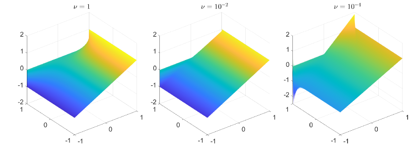
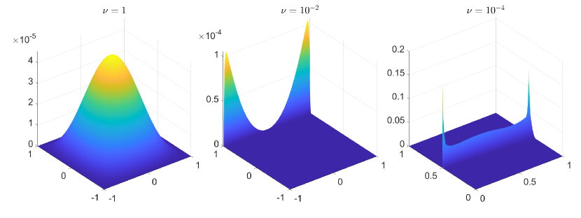
Figure 1: Example 6.1: Mean (top) and variance (bottom) of SG solutions obtained solving by $\mathcal{A}\backslash\mathcal{F}$ with $\ell=1$, $\kappa=0.05$, $N_{d}=393216$, $N=3$, and $Q=2$ for various values of viscosity parameter $\nu$.

Table 1: Example 6.1: Simulation results showing ranks of truncated solutions, total number of iterations, total CPU times (in seconds), relative residual, and memory demand of the solution (in KB) with $N_{d}=6144$, $Q=3$, $\ell=1$, $\kappa=0.05$, $\nu=10^{-4}$, and the mean-based preconditioner $\mathcal{P}_{0}$ for varying values of $N$.

Method $\epsilon_{trunc}$	LRPCG 1e-06 (1e-08)	LRPBiCGstab 1e-06 (1e-08)	LRPQMRCGstab 1e-06 (1e-08)	LRPGMRES 1e-06 (1e-08)
N=3
Ranks	10 (10)	10 (10)	9 (10)	10 (10)
#iter	5 (5)	3 (3)	3 (3)	4 (4)
CPU	7.0 (7.7)	8.8 (8.9)	7.8 (10.0)	5.4 (5.2)
Resi.	1.8160e-07 (3.2499e-07)	5.5982e-06 (5.5413e-06)	2.9222e-05 (3.1021e-05)	6.3509e-07 (6.3509e-07)
Memory	481.6 (481.6)	481.6 (481.6)	433.4 (481.6)	481.6 (481.6)
N=4
Ranks	12 (18)	17 (18)	17 (17)	17 (17)
#iter	4 (5)	3 (3)	3 (3)	5 (5)
CPU	9.2 (13.3)	15.3 (15.3)	14.2 (14.4)	12.1 (11.7)
Resi.	1.2367e-06 (1.4311e-07)	7.7090e-06 (7.7030e-06)	1.0819e-05 (4.3167e-06)	8.1316e-08 (8.1316e-08)
Memory	579.3 (868.9)	820.7 (868.9)	820.7 (820.7)	820.7 (820.7)
N=5
Ranks	18 (28)	21 (28)	22 (28)	19 (28)
#iter	4 (5)	3 (3)	3 (3)	5 (5)
CPU	15.2 (20.8)	24.9 (25.1)	25.4 (26.0)	20.3 (20.6)
Resi.	1.1705e-06 (8.2045e-08)	8.5525e-06 (8.5527e-06)	1.6985e-06 (8.6182e-07)	8.4680e-08 (8.4680e-08)
Memory	871.9 (1356.3)	1017.2 (1356.3)	1065.6 (1356.3)	920.3 (1356.3)
N=6
Ranks	26 (42)	26 (42)	25 (42)	25 (42)
#iter	4 (4)	3 (3)	3 (3)	4 (4)
CPU	25.6 (32.0)	42.4 (43.7)	49.4 (51.2)	29.7 (31.5)
Resi.	9.2495e-07 (1.0605e-06)	9.6694e-06 (9.6649e-06)	7.7812e-07 (4.1770e-07)	1.0476e-06 (1.0476e-06)
Memory	1265.1 (2043.6)	1265.1 (2043.6)	1216.4 (2043.6)	1216.4 (2043.6)
N=7
Ranks	30 (60)	32 (60)	32 (60)	28 (47)
#iter	4 (4)	3 (3)	3 (3)	4 (4)
CPU	52.5 (58.8)	69.3 (73.8)	86.1 (87.9)	57.9 (57.7)
Resi.	1.0719e-06 (1.1205e-06)	9.9865e-06 (9.9880e-06)	6.5595e-07 (2.0226e-07)	1.1075e-06 (1.1075e-06)
Memory	1468.1 (2936.3)	1566 (2936.3)	1566 (2936.3)	1370.3 (2300.1)

When $N$ increases, the complexity of the problem increases. As expected, decreasing the truncation tolerance $\epsilon_{trunc}$ increases the cost of computational time and memory requirement, especially for large $N$. Another key observation from the Table 1 is that LRPGMRES exhibits better performance compared to other iterative solvers in terms of CPU time and memory requirement. Table  2 displays the performance of low–rank of Krylov subspace methods with the mean–based preconditioner $\mathcal{P}_{0}$ for varying viscosity parameter $\nu$. Decreasing the values of $\nu$ makes the problem more convection dominated. Thus, the rank of the low–rank solution and memory requirements increase for all iterative solvers.

Table 2: Example 6.1: Simulation results showing ranks of truncated solutions, total number of iterations, total CPU times (in seconds), relative residual, and memory demand of the solution (in KB) with $N_{d}=6144$, $Q=3$, $\ell=1$, $\kappa=0.05$, $N=7$, and the mean-based preconditioner $\mathcal{P}_{0}$ for various values of viscosity parameter $\nu$.

Method $\epsilon_{trunc}$	LRPCG 1e-06 (1e-08)	LRPBiCGstab 1e-06 (1e-08)	LRPQMRCGstab 1e-06 (1e-08)	LRPGMRES 1e-06 (1e-08)
$\nu=1$
Ranks	17 (44)	20 (51)	20 (42)	22 (39)
#iter	4 (4)	3 (3)	3 (3)	4 (4)
CPU	54.3 (62.0)	68.7 (75.2)	87.9 (91.2)	56.4 (56.3)
Resi.	8.2189e-07 (1.1215e-06)	9.9896e-06 (9.9897e-06)	7.3503e-07 (3.6458e-08)	1.1062e-06 (1.1062e-06)
Memory	831.9 (2300.1)	978.8 (2495.8)	978.8 (2055.4)	1076.6 (1908.6)
$\nu=10^{-2}$
Ranks	21 (60)	26 (60)	25 (59)	23 (39)
#iter	4 (4)	3 (3)	3 (3)	4 (4)
CPU	52.4 (64.5)	65.9 (72.3)	89.5 (94.3)	52.3 (52.6)
Resi.	7.7284e-07 (1.1225e-06)	9.9906e-06 (9.9918e-06)	1.6268e-06 (8.4171e-08)	1.1074e-06 (1.1074e-06)
Memory	1027.7 (2936.3)	1272.4 (2936.3)	1223.4 (2887.3)	1125.6 (1908.6)
$\nu=10^{-4}$
Ranks	30 (60)	32 (60)	32 (60)	28 (47)
#iter	4 (4)	3 (3)	3 (3)	4 (4)
CPU	52.5 (58.8)	69.3 (73.8)	86.1 (87.9)	57.9 (57.7)
Resi.	1.0719e-06 (1.1205e-06)	9.9865e-06 (9.9880e-06)	6.5595e-07 (2.0226e-07)	1.1075e-06 (1.1075e-06)
Memory	1468.1 (2936.3)	1566 (2936.3)	1566 (2936.3)	1370.3 (2300.1)

Next, we investigate the convergence behavior of the low–rank variants of iterative solvers with different values of standard deviation $\kappa$ for varying values of $\nu$ in Figure 2. For relatively large $\kappa$, we observe that LRPBiCGstab and LRPGMRES yield better convergence behaviour, whereas the LRPCG method does not converge since the dominance of nonsymmetrical increases.

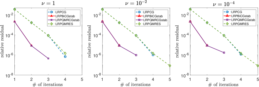
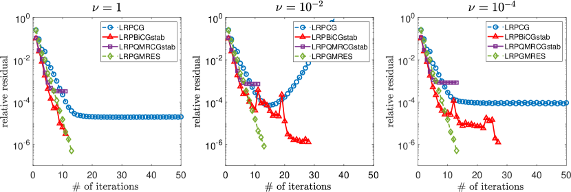
Figure 2: Example 6.1: Convergence of low–rank variants of iterative solvers with $\kappa=0.05$ (top) and $\kappa=0.5$ (bottom) for varying values of viscosity $\nu$. The mean-based preconditioner $\mathcal{P}_{0}$ is used with the parameters $N=5$, $Q=3$, $\ell=1$, $N_{d}=6144$, and $\epsilon_{trunc}=10^{-6}$.

Table 3: Example 6.1: Simulation results showing ranks of truncated solutions, total number of iterations, total CPU times (in seconds), relative residual, and memory demand of the solution (in KB) with $N_{d}=6144$, $N=7$, $Q=3$, $\ell=1$, $\epsilon_{trunc}=10^{-6}$, and $\nu=10^{-4}$ for different choices of preconditioners.

Method Preconditioner	LRPBiCGstab $\mathcal{P}_{0}$	LRPGMRES $\mathcal{P}_{0}$	LRPBiCGstab $\mathcal{P}_{1}$	LRPGMRES $\mathcal{P}_{1}$
$\kappa=0.05$
Ranks	32	28	31	27
#iter	3	4	3	5
CPU	69.3	57.9	69.0	72.7
Resi.	9.9865e-06	1.1075e-06	6.0448e-06	8.7712e-08
Memory	1566	1370.3	1517.1	1321.3
$\kappa=0.5$
Ranks	60	60	60	60
#iter	13	13	15	13
CPU	781.7	248.5	913.6	245.8
Resi.	1.2629e-06	4.9417e-07	1.8697e-06	6.9625e-07
Memory	2936.3	2936.3	2936.3	2936.3

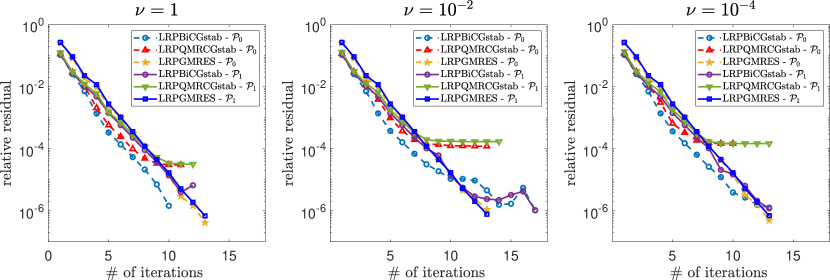
Figure 3: Example 6.1: Convergence of low–rank variants of LRPBiCGstab, LRPQMRCGstab, and LRPGMRES with $N=7$, $Q=3$, $\ell=1$, $N_{d}=6144$, $\epsilon_{trunc}=10^{-8}$, and $\kappa=0.5$ for the mean-based preconditioner $\mathcal{P}_{0}$ and the Ullmann preconditioner $\mathcal{P}_{1}$.

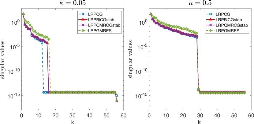
Figure 4: Example 6.1: Decay of singular values of low–rank solution matrix $\mathbf{U}$ obtained by using the mean-based preconditioner $\mathcal{P}_{0}$ with $N=5$, $Q=3$, $\ell=1$, $N_{d}=6144$, $\nu=1$, and $\epsilon_{trunc}=10^{-6}$ for $\kappa=0.05$ (left) and $\kappa=0.5$ (right).

In Table 3, we examine the effect of the standard deviation parameter $\kappa$ with $\mathcal{P}_{0}$ and $\mathcal{P}_{1}$ preconditioners for only LRPBiCGstab and LRPGMRES since they exhibit better convergence behaviour; see Figure 2. As $\kappa$ increases, the low-rank solutions indicate deteriorating performance, regardless of which the preconditioner or iterative solver are used. We also examine the effect of preconditioners on the iterative solvers in Figure 3 in terms of convergence of iterative solvers. Since LRPCG does not converge for large values of $\kappa$, they are not included. The results show that the mean–based preconditioner $\mathcal{P}_{0}$ exhibits better convergence behaviour compared to the Ullmann preconditioner $\mathcal{P}_{1}$ for LRPBiCGstab and LRPQMRCGstab, whereas they are almost the same for LRPGMRES.

Figure 4 shows the decay of singular values of low–rank solution matrix $\mathbf{U}$ obtained by using the mean-based preconditioner $\mathcal{P}_{0}$. Keeping other parameters fixed, increasing the value of $\kappa$ slows down the decay of the singular values of the obtained solutions. Thus, the total time for solving the system and the time spent on truncation will also increase; see Table 3.

Table 4: Example 6.1: Total CPU times (in seconds) and memory (in KB) for $N_{d}=6144$, $Q=3$, $\ell=1$, and $\kappa=0.05$.

$\mathcal{A}\backslash\mathcal{F}$	$\nu=10^{0}$	$\nu=10^{-2}$	$\nu=10^{-4}$
N	CPU (Memory)	CPU (Memory)	CPU (Memory)
2	10.8 (960)	10.7 (960)	10.8 (960)
3	1463.7 (1920)	1464.2 (1920)	1463.7 (1920)
4	OoM	OoM	OoM

Last, we display the performance of $\mathcal{A}\backslash\mathcal{F}$ in terms of total CPU times (in seconds) and memory requirements (in KB) in Table 4. Some numerical results are not reported since the solution from terminates with ”out of memory”, which we have denoted as ”OoM”. A major observation from numerical simulations, low–rank variant of Krylov subspace methods achieve greater computational savings especially in terms of memory.

6.2 Stationary problem with random convection parameter

Our second example is a two-dimensional stationary convection diffusion equation with random velocity. To be precise, we choose the deterministic diffusion parameter $a(x,\omega)=\nu>0$, the deterministic source function $f(x)=0$, and the spatial domain $\mathcal{D}=[0,1]^{2}$. The random velocity field $\mathbf{b}(x,\omega)$ is

$$\mathbf{b}(x,\omega):=\left(\cos\Big{(}\frac{1}{5}\eta(x,\omega)\Big{)},\sin\Big{(}\frac{1}{5}\eta(x,\omega)\Big{)}\right)^{T},$$ (36)

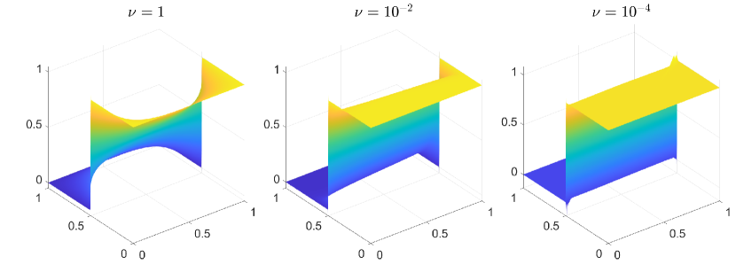
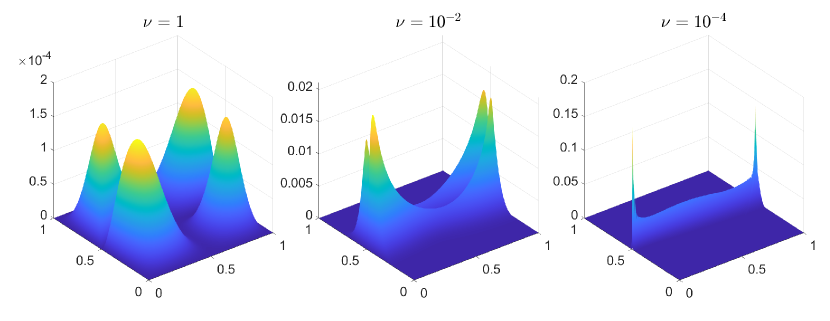
Figure 5: Example 6.2: Mean (top) and variance (bottom) of SG solutions obtained by solving $\mathcal{A}\backslash\mathcal{F}$ with $N=2$, $Q=2$, $\ell=1$, $N_{d}=393216$, and $\kappa=0.05$, for various values of $\nu$.

where the random field $\eta(x,\omega)$ is chosen as a uniform random field having zero mean with the covariance function defined in (35). The Dirichlet boundary condition $u_{d}(x)$ is given by

$$u_{d}(x)=\begin{cases}1,&x\in S,\\ 0,&x\in\partial\mathcal{D}\backslash S,\end{cases}$$

where the set $S$ is the subset of $\partial\mathcal{D}$ defined by

$$\{x_{1}=0,x_{2}\in[0,0.5]\}\cup\{x_{1}\in[0,1],x_{2}=0\}\cup\{x_{1}=1,x_{2}\in[0,0.5]\}.$$

Due to the random velocity, $\mathbf{b}(x,\omega)$, the solution has sharp transitions in the domain $\mathcal{D}$ and then spurious oscillations will propagate into the stochastic domain $\Omega$. As $\nu$ decreases, the interior layer becomes more visible; see Figure 5 for the mean and variance of solution for various values of $\nu$.

Table 5: Example 6.2: Simulation results showing ranks of truncated solutions, total number of iterations, total CPU times (in seconds), relative residual, and memory demand of the solution (in KB) with $N_{d}=6144$, $Q=3$, $\ell=1$, $\kappa=0.05$, $N=7$, and the mean-based preconditioner $\mathcal{P}_{0}$ for various values of viscosity parameter $\nu$.

Method $\epsilon_{trunc}$	LRPCG 1e-06 (1e-08)	LRPBiCGstab 1e-06 (1e-08)	LRPQMRCGstab 1e-06 (1e-08)	LRPGMRES 1e-06 (1e-08)
$\nu=1$
Ranks	8 (19)	10 (23)	9 (22)	6 (8)
#iter	10 (10)	3 (3)	4 (4)	5 (5)
CPU	108.6 (120.4)	49.7 (56.0)	76.1 (82.4)	60.7 (59.7)
Resi.	1.3666e-06 (1.4307e-06)	5.7868e-07 (5.7870e-07)	6.8606e-06 (6.8424e-06)	1.2811e-06 (1.2811e-06)
Memory	391.5 (929.8)	489.4 (1125.6)	440.4 (1076.6)	293.6 (391.5)
$\nu=10^{-2}$
Ranks	15 (34)	45 (60)	21 (60)	6 (14)
#iter	100 (100)	100 (100)	100 (100)	100 (100)
CPU	992.2 (1202.8)	1782.7 (2133.9)	2602.3 (2815.0)	8798.7 (8864.7)
Resi.	3.0059e+26 (3.0060e+26)	1.4807e-01 (2.6669e-02)	9.0173e-03 (9.3659e-03)	1.0002e-03 (1.0002e-03)
Memory	734.1 (1663.9)	2202.2 (2936.3)	1027.7 (2936.3)	293.6 (685.1)
$\nu=10^{-4}$
Ranks	29 (60)	60 (60)	35 (60)	12 (27)
#iter	100 (100)	100 (100)	100 (100)	100 (100)
CPU	1102.3 (1382.6)	2124.4 (2135.5)	2802.1 (2869.9)	8401.0 (8394.8)
Resi.	8.7243e+26 (8.7242e+26)	2.2085e-02 (3.2792e-02)	3.6713e-03 (3.3074e-03)	1.2075e-03 (1.2075e-03)
Memory	1419.2 (2936.3)	2936.3 (2936.3)	1712.8 (2936.3)	587.3 (1321.3)

In Table 5 and  6, we display the performance of low–rank of Krylov subspace methods with the mean–based precondition $\mathcal{P}_{0}$ by considering various data sets. When $\nu$ decreases, the complexity of the problem increases in terms of the rank of the truncated solutions, total CPU times (in seconds), and memory demand of the solution (in KB); see Table 5. As the previous example, LRPCG method does not work well for smaller values of $\nu$, whereas LRPGMRES exhibits better performance. Next, we investigate the convergence behavior of the low–rank variants of iterative solvers with different values of $\nu$ in Figure 6. While LRPBiCGstab method exhibits oscillatory behaviour, the relative residuals obtained by LRPQMRCGstab and LRPGMRES decrease monotonically.

Table 6: Example 6.2: Simulation results showing ranks of truncated solutions, total number of iterations, total CPU times (in seconds), relative residual, and memory demand of the solution (in KB) with $N=7$, $Q=3$, $\ell=1$, $\kappa=0.05$, $\nu=10^{-4}$ and the mean-based preconditioner $\mathcal{P}_{0}$ for various values of $N_{d}$.

	LRPCG 1e-06 (1e-08)	LRPBiCGstab 1e-06 (1e-08)	LRPQMRCGstab 1e-06 (1e-08)	LRPGMRES 1e-06 (1e-08)
$N_{d}=384$
Ranks	17 (37)	58 (60)	21 (60)	26 (42)
#iter	100 (100)	100 (100)	100 (100)	100 (100)
CPU	213.3 (205.7)	329.8 (329.4)	487.6 (481.7)	2119.7 (2135.3)
Resi.	1.1637e+28 (1.1637e+28)	1.5964e-02 (3.3908e-01)	1.0163e-02 (1.0857e-02)	7.4718e-06 (7.2284e-06)
Memory	66.9 (145.7)	228.4 (236.3)	82.7 (236.3)	102.4 (165.4)
$N_{d}=1536$
Ranks	25 (56)	60 (60)	21 (55)	30 (49)
#iter	100 (100)	100 (100)	100 (100)	65 (65)
CPU	305.4 (338.8)	497.8 (503.0)	699.4 (709.0)	1278.3 (1286.1)
Resi.	2.9340e+27 (2.9339e+27)	5.3887e-02 (1.9615e-02)	6.8316e-03 (7.0652e-03)	1.8606e-06 (1.8606e-06)
Memory	323.4 (724.5)	776.3 (776.3)	271.7 (711.6)	388.1 (633.9)
$N_{d}=6144$
Ranks	29 (60)	60 (60)	35 (60)	12 (27)
#iter	100 (100)	100 (100)	100 (100)	100 (100)
CPU	1102.3 (1382.6)	2124.4 (2135.5)	2802.1 (2869.9)	8401.0 (8394.8)
Resi.	8.7243e+26 (8.7242e+26)	2.2085e-02 (3.2792e-02)	3.6713e-03 (3.3074e-03)	1.2075e-03 (1.2075e-03)
Memory	1419.2 (2936.3)	2936.3 (2936.3)	1712.8 (2936.3)	587.3 (1321.3)
$N_{d}=24576$
Ranks	25 (60)	60 (60)	23 (60)	7 (19)
#iter	100 (100)	100 (100)	100 (100)	100 (100)
CPU	7276.2 (10498.6)	16726.6 (16936.7)	19960.3 (20646.5)	41929.8 (41778.9)
Resi.	3.5040e+26 (3.5100e+26)	5.8952e-03 (1.7120e-02)	1.7710e-03 (1.6015e-03)	7.3550e-04 (7.3550e-04)
Memory	4823.4 (11576.3)	11576.3 (11576.3)	4437.6 (11576.2)	1350.6 (3665.8)

Figure 7 shows the decay of singular values of low–rank solution matrix $\mathbf{U}$ obtained by using $\mathcal{P}_{0}$ and $\mathcal{P}_{1}$ preconditioners. Keeping other parameters fixed, decreasing the value of $\nu$ slows down the decay of the singular values of the obtained solutions. Thus, the total time for solving the system and the time spent on truncation will increase; see Table 5. In practical applications, one is usually more interested in large–scale simulations in which the degree of freedom (Dof) is quite large. In Table 7, we look for memory demand of the solution (in KB) obtained full–rank and low–rank variants of GMRES solver. As expected, low–rank approximation significantly reduces computer memory required to solve the large system.

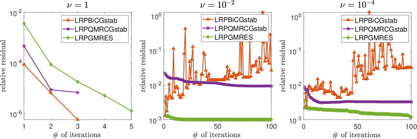
Figure 6: Example 6.2: Convergence of low–rank variants of iterative solvers for varying values of viscosity $\nu$. The mean-based preconditioner $\mathcal{P}_{0}$ is used with the parameters $N=7$, $Q=3$, $\ell=1$, $\kappa=0.05$, $N_{d}=6144$, and $\epsilon_{trunc}=10^{-8}$.

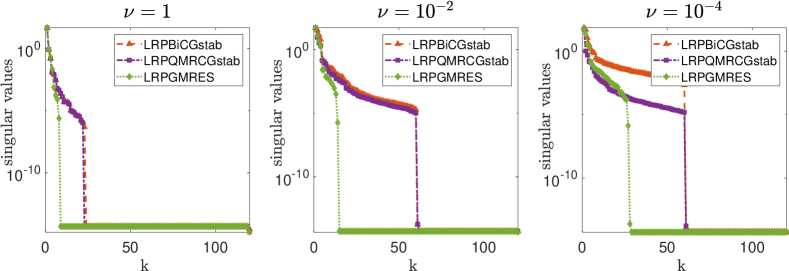
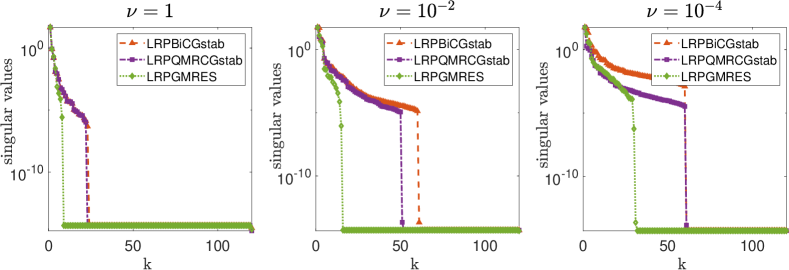
Figure 7: Example 6.2: Decay of singular values of solution matrix $\mathbf{U}$ with $N=7$, $Q=3$, $\ell=1$, $N_{d}=6144$, $\kappa=0.05$, and $\epsilon_{trunc}=10^{-8}$ with the mean-based preconditioner (top) and the Ullmann preconditioner (bottom) for various values of $\nu$.

Table 7: Example 6.2: Memory demand of the solution (in KB) obtained full–rank and low–rank variants of GMRES solver with $N=7$, $Q=3$, $\ell=1$, $\kappa=0.05$, $\epsilon_{trunc}=10^{-6}$ ($\epsilon_{trunc}=10^{-8}$), and the mean-based preconditioner $\mathcal{P}_{0}$ for various values of degree of freedom (DoF).

DoF	46080	184320	737280	2949120
Low–Rank	94.5 (157.5)	323.4 (556.3)	587.3 (1468.1)	1543.5 (3665.8)
Full–Rank	360	1440	5760	23040

6.3 Unsteady problem with random diffusion parameter

Last, we consider an unsteady convection diffusion equation with random diffusion parameter defined on $\mathcal{D}=[0,1]^{2}$. The rest of data is as follows

$$T=0.5,\quad\mathbf{b}(x)=(1,1)^{T},\quad f(x,t)=0,\quad u^{0}(x)=0$$

with the Dirichlet boundary condition

$$u_{d}(x)=\begin{cases}u_{d}(0,x_{2})=x_{2}(1-x_{2}),&u_{d}(1,x_{2})=0,\\ u_{d}(x_{1},0)=0,&u_{d}(x_{1},1)=0.\end{cases}$$

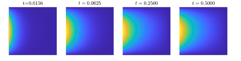
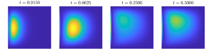
Figure 8: Example 6.3: Mean and variance of computed solution at various time steps obtained by LRPBiCGstab with $N=17$, $Q=3$, $\ell=1.5$, $\sigma=0.15$, $\epsilon_{trunc}=10^{-6}$, and $\mathcal{P}_{0}$.

Table 8: Example 6.3: Simulation results showing ranks of truncated solutions, total number of iterations, total CPU times (in seconds), relative residual, and memory demand of the solution (in KB) with $N_{d}=6144$, $Q=3$, $\kappa=0.15$, and the mean-based preconditioner $\mathcal{P}_{0}$ for various values of correlation length $\ell$ at final time $T=0.5$.

Method $\epsilon_{trunc}$	LRPCG 1e-06 (1e-08)	LRPBiCGstab 1e-06 (1e-08)	LRPQMRCGstab 1e-06 (1e-08)	LRPGMRES 1e-06 (1e-08)
$\ell=3$, $N=9$
Ranks	25 (56)	25 (55)	22 (52)	25 (38)
#iter	4 (4)	3 (3)	4 (4)	4 (4)
CPU	5348.9 (6543.5)	5072.2 (6869.4)	9459.5 (11060.9)	5974.5 (6005.6)
Resi.	2.7590e-04 (2.7601e-04)	1.2268e-03 (1.2268e-03)	8.5901e-05 (8.5657e-05)	2.3936e-04 (2.3936e-04)
Memory	1243 (2784.3)	1243 (2734.5)	1093.8 (2585.4)	1243 (1889.3)
$\ell=2.5$, $N=10$
Ranks	27 (61)	27 (60)	25 (55)	27 (43)
#iter	4 (4)	3 (3)	4 (4)	4 (4)
CPU	7564.4 (9310.7)	7030.5 (9558.5)	13158.6 (15636.3)	9219.1 (9158.8)
Resi.	2.7397e-04 (2.7405e-04)	1.2665e-03 (1.2665e-03)	9.5085e-05 (9.4831e-05)	2.3810e-04 (2.3810e-04)
Memory	1356.3 (3064.3)	1356.3 (3014.1)	1255.7 (2762.9)	1356.3 (2160.1)
$\ell=2$, $N=13$
Ranks	28 (68)	29 (66)	27 (63)	32 (52)
#iter	4 (4)	3 (3)	4 (4)	4 (4)
CPU	10813.5 (15435.4)	10745.0 (15709.9)	18748.2 (24049.6)	18496.9 (18284.7)
Resi.	2.6686e-04 (2.6703e-04)	1.2994e-03 (1.2994e-03)	1.0372e-04 (1.0345e-04)	2.4580e-04 (2.4580e-04)
Memory	1466.5 (3561.5)	1518.9 (3456.8)	1414.1 (3299.6)	1676 (2723.5)
$\ell=1.5$, $N=17$
Ranks	32 (78)	33 (77)	31 (73)	38 (62)
#iter	4 (4)	3 (3)	4 (4)	4 (4)
CPU	20658.3 (36422.4)	22889.2 (33851.9)	36876.4 (50963.2)	58974.4 (57828.0)
Resi.	2.3545e-04 (2.3548e-04)	1.3217e-03 (1.3217e-03)	1.0444e-04 (1.0425e-04)	2.9531e-04 (2.9531e-04)
Memory	1821 (4438.7)	1877.9 (4381.8)	1764.1 (4154.2)	2162.4 (3528.2)

The random diffusion coefficient $a(x,w)$ is a uniform random field having unity mean with the covariance function (35). In the numerical simulations, the number of time points is chosen as $N_{T}=32$. From literature, see, e.g., [33], we know that decreasing the correlation length slows down the decay of the eigenvalues in the KL expansion of the random variable $a(\mathbf{x},\omega)$ and therefore, more random variables are required to sufficiently capture the randomness. That is, it results in an increase in the truncation parameter $N$: The reverse is the case when the correlation length is increased. Therefore, the effect of correction length on the low–rank variants of the iterative solver is our main focus for this benchmark problem. With the help of the following computation as done in [14],

$$\left(\sum\limits_{i=1}^{N}\lambda_{i}\right)/\left(\sum\limits_{i=1}^{M_{\ell}}\lambda_{i}\right)>0.97,$$

we can compute suitable truncation number $N$ for the given correlation length $\ell$. Here, $M_{\ell}$ is a large number which we set $1000$. Computed mean and variance of the solution are displayed in Figure 8 for various time steps.

Table 9: Example 6.3: Simulation results showing total number of iterations, total CPU times (in seconds), and memory demand of the full–rank solution (in KB) with $N_{d}=6144$, $Q=3$, $\kappa=0.15$, and the mean-based preconditioner $\mathcal{P}_{0}$ for various values of correlation length $\ell$ at final time $T=0.5$.

Method $\epsilon_{tol}$	PCG 1e-04	PBiCGstab 1e-04	PGMRES 1e-04
$\ell=3$, $N=9$
#iter	11	5.5	10
CPU	7910.7	7863.4	8727.0
Memory	10560	10560	10560
$\ell=2$, $N=13$
#iter	11	5.5	10
CPU	20252.0	20148.5	22318.8
Memory	26880	26880	26880
$\ell=1.5$, $N=17$
#iter	11	5.5	10
CPU	41345.0	41207.4	45499.8
Memory	54720	54720	54720

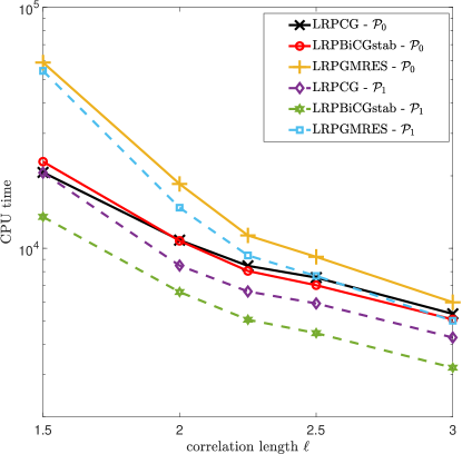
Figure 9: Example 6.3: CPU times of LRPCG, LRPBiCGstab, and LRPGMRES iterative solvers obtained by the preconditioners $\mathcal{P}_{0}$ and $\mathcal{P}_{1}$ with $Q=3$, $N_{d}=6144$, and $\kappa=0.15$ for various values of correlation length $\ell$.

Table 8 displays the results of numerical simulations for the mean-based preconditioner $\mathcal{P}_{0}$ for varying values of the correlation length $\ell$. Provided that $97\%$ of the total variance is captured, the small correlation length increases the rank of the computed low–rank solutions and the number of iterations regardless of which the iterative solver is used. Another observation is that decreasing the truncation tolerance $\epsilon_{trunc}$ does not affect the relative residuals but, as expected, at the cost of comparatively more computational time and memory requirements. Next, numerical results obtained by using the standard Krylov subspace iterative solvers with the mean-based preconditioner $\mathcal{P}_{0}$ are displayed in Table 9. Compared to the full–rank solvers in Table 9, low–rank Krylov subspace solvers generally exhibit better performance; see Table 8. Regarding of the preconditioners, Ullmann preconditioner $\mathcal{P}_{1}$ produce better performance in terms of computational time; see Figure 9.

7 Conclusions

In this paper, we have numerically studied the statistical moments of a convection diffusion equation having random coefficients. With the help of the stochastic Galerkin approach, we transform the original problem into a system consisting of deterministic convection diffusion equations for each realization of random coefficients. Then, the symmetric interior penalty Galerkin method is used to discretize the deterministic problems due to its local mass conservativity. To reduce computational time and memory requirements, we have used low–rank variants of various Krylov subspace methods, such as CG, BiCGstab, QMRCGstab, and GMRES with suitable preconditioners. It has been shown in the numerical simulations that LRPGMRES exhibits better performance, especially for convection dominated models.

Appendix A Proof of Theorem 3.2

By choosing $\widetilde{v}=\Pi_{n}(\mathcal{R}_{h}(v))$, we obtain

$$\lVert v-\widetilde{v}\rVert_{L^{2}(H^{1}(\mathcal{D});\Gamma)} \leq \lVert v-\mathcal{R}_{h}(v)\rVert_{L^{2}(H^{1}(\mathcal{D});\Gamma)}+\lVert\mathcal{R}_{h}(v)-\Pi_{n}(\mathcal{R}_{h}(v))\rVert_{L^{2}(H^{1}(\mathcal{D});\Gamma)}$$

$$= \lVert v-\mathcal{R}_{h}(v)\rVert_{L^{2}(H^{1}(\mathcal{D});\Gamma)}+\lVert\mathcal{R}_{h}(v-\Pi_{n}(v))\rVert_{L^{2}(H^{1}(\mathcal{D});\Gamma)}$$

for a fixed $v\in L^{2}(H^{2}(\mathcal{D});\Gamma)\cap H^{q+1}(H^{1}(\mathcal{D});\Gamma)$. In view of the estimate in (27), we have

$$\lVert v-\mathcal{R}_{h}(v)\rVert_{L^{2}(H^{1}(\mathcal{D});\Gamma)}\leq Ch^{\min(\ell+1,2)-1}\lVert v\rVert_{L^{2}(H^{2}(\mathcal{D});\Gamma)}.$$ (37)

With the help of the $H^{1}$–projection operator in (24a), the Cauchy–Schwarz inequality, the $L^{2}$–projection operator in (23), and the approximation in (22), we obtain

$$\lVert\mathcal{R}_{h}(v-\Pi_{n}(v))\rVert_{L^{2}(H^{1}(\mathcal{D});\Gamma)} \leq C\lVert v-\Pi_{n}(v)\rVert_{L^{2}(H^{1}(\mathcal{D});\Gamma)}$$ (38)

$$\leq C\sum_{n=1}^{N}\bigg{(}\frac{k_{n}}{2}\bigg{)}^{q_{n}+1}\dfrac{\lVert\partial^{q_{n}+1}_{\xi_{n}}v\rVert_{L^{2}(H^{1}(\mathcal{D});\Gamma)}}{(q_{n}+1)!}.$$

Combining (37) and (38), we get

$$\lVert v-\widetilde{v}\rVert_{L^{2}(H^{1}(\mathcal{D});\Gamma)} \leq Ch^{\min(\ell+1,2)-1}\lVert v\rVert_{L^{2}(H^{2}(\mathcal{D});\Gamma)}$$

$$+\sum_{n=1}^{N}\bigg{(}\frac{k_{n}}{2}\bigg{)}^{q_{n}+1}\dfrac{\lVert\partial^{q_{n}+1}_{\xi_{n}}v\rVert_{L^{2}(H^{1}(\mathcal{D});\Gamma)}}{(q_{n}+1)!},$$

which implies (28a). For the derivation of (28b), we follow the same strategy:

$$\lVert\nabla^{2}(v-\widetilde{v})\rVert_{L^{2}(L^{2}(\mathcal{D});\Gamma)}$$

$$\qquad\leq\lVert\nabla^{2}(v-\mathcal{R}_{h}(v))\rVert_{L^{2}(L^{2}(\mathcal{D});\Gamma)}+\lVert\nabla^{2}(\mathcal{R}_{h}(v)-\Pi_{n}(\mathcal{R}_{h}(v))\rVert_{L^{2}(L^{2}(\mathcal{D});\Gamma)}$$

$$\qquad=\lVert\nabla^{2}(v-\mathcal{R}_{h}(v))\rVert_{L^{2}(L^{2}(\mathcal{D});\Gamma)}+\lVert\nabla^{2}(\mathcal{R}_{h}(v-\Pi_{n}(v))\rVert_{L^{2}(L^{2}(\mathcal{D});\Gamma)}.$$

An application of the inverse inequality (26) on $\mathcal{R}_{h}(v)$, the definition of $H^{1}$–projection operator (24a), and the Cauchy–Schwarz inequality yields

$$\lVert\nabla^{2}(\mathcal{R}_{h}(v))\rVert_{L^{2}(\mathcal{D})}\leq Ch^{-1}\lVert\nabla(\mathcal{R}_{h}(v))\rVert_{L^{2}(\mathcal{D})}\leq Ch^{-1}\lVert\nabla v\rVert_{L^{2}(\mathcal{D})}.$$ (39)

By (22), (39), and (27),

$$\lVert\nabla^{2}(v-\tilde{v})\rVert_{L^{2}(L^{2}(\mathcal{D});\Gamma)} \leq \lVert\nabla^{2}(v-\mathcal{R}_{h}(v))\rVert_{L^{2}(L^{2}(\mathcal{D});\Gamma)}$$

$$+Ch^{-1}\lVert\nabla(v-\Pi_{n}(v))\rVert_{L^{2}(\mathcal{D};\Gamma)}$$

$$\leq Ch^{\min(\ell+1,2)-2}\lVert v\rVert_{L^{2}(H^{2}(\mathcal{D});\Gamma)}$$

$$+Ch^{-1}\sum_{n=1}^{N}\bigg{(}\frac{k_{n}}{2}\bigg{)}^{q_{n}+1}\dfrac{\lVert\partial^{q_{n}+1}_{\xi_{n}}v\rVert_{L^{2}(H^{1}(\mathcal{D});\Gamma)}}{(q_{n}+1)!},$$

which is the desired result.

Appendix B Proof of Theorem 3.3

Decompose $\lVert u-u_{h}\rVert_{\xi}$ as

$$\lVert u-u_{h}\rVert_{\xi}\leq\lVert u_{h}-\widetilde{u}\rVert_{\xi}+\lVert u-\widetilde{u}\rVert_{\xi},$$ (40)

where $\widetilde{u}\in V_{h}\otimes\mathcal{Y}_{k}^{q}$ is an approximation of the solution $u$, satisfying the Theorem 3.2.

Now, we first find a bound for the first term of (40). By the coercivity of the bilinear form (17a), the Galerkin orthogonality, an integration by parts over convective term in the bilinear form (15), and the assumption on the convective term $\nabla\cdot\mathbf{b}=0$, we obtain

$$c_{cv}\lVert u_{h}-\widetilde{u}\rVert_{\xi}^{2} \leq a_{\xi}(u_{h}-\widetilde{u},u_{h}-\tilde{u})$$ (41)

$$= a_{\xi}(u-\widetilde{u},\underbrace{u_{h}-\tilde{u}}_{\chi\in V_{h}})+\underbrace{a_{\xi}(u-u_{h},u_{h}-\widetilde{u})}_{=0}$$

$$= \int\limits_{\Gamma}\rho(\xi)\Bigg{[}\sum\limits_{K\in\mathcal{T}_{h}}\int\limits_{K}a\nabla(u-\widetilde{u})\cdot\nabla\chi\;dx-\sum\limits_{E\in\mathcal{E}^{0}_{h}\cup\mathcal{E}_{h}^{\partial}}\int\limits_{E}\mbox{$\left\{\!\!\left\{a\nabla(u-\widetilde{u})\right\}\!\!\right\}$}\mbox{$\left[\!\left[\chi\right]\!\right]$}\;ds$$

$$-\sum\limits_{E\in\mathcal{E}^{0}_{h}\cup\mathcal{E}_{h}^{\partial}}\int\limits_{E}\mbox{$\left\{\!\!\left\{a\nabla\chi\right\}\!\!\right\}$}\mbox{$\left[\!\left[u-\widetilde{u}\right]\!\right]$}\;ds+\sum\limits_{E\in\mathcal{E}^{0}_{h}\cup\mathcal{E}_{h}^{\partial}}\frac{\sigma}{h_{E}}\int\limits_{E}\mbox{$\left[\!\left[u-\widetilde{u}\right]\!\right]$}\cdot\mbox{$\left[\!\left[\chi\right]\!\right]$}\;ds$$

$$-\sum\limits_{K\in\mathcal{T}_{h}}\int\limits_{K}\mathbf{b}\cdot(u-\tilde{u})\nabla\chi\;dx-\sum\limits_{K\in\mathcal{T}_{h}}\;\int\limits_{\partial K^{+}\backslash\partial\mathcal{D}}\mathbf{b}\cdot\mathbf{n_{E}}(u-\tilde{u})(\chi^{e}-\chi)\;ds$$

$$+\sum\limits_{K\in\mathcal{T}_{h}}\;\int\limits_{\partial K^{+}\cap\mathcal{D}^{+}}\mathbf{b}\cdot\mathbf{n_{E}}(u-\tilde{u})\chi\;ds\Bigg{]}d\xi$$

$$\leq \lvert T_{1}+T_{2}+T_{3}+T_{4}+T_{5}+T_{6}+T_{7}\rvert.$$

With the help of the bound on $a(x,\omega)$ (3), Cauchy–Schwarz inequality, Young’s inequality, and Theorem 3.2, we obtain the following bound for the first term in (41)

$$\lvert T_{1}\rvert \leq \int\limits_{\Gamma}\rho\sqrt{a_{\max}}\Bigg{(}\sum\limits_{K\in\mathcal{T}_{h}}\lVert\nabla(u-\widetilde{u})\rVert^{2}_{L^{2}(K)}\Bigg{)}^{\frac{1}{2}}\Bigg{(}\sum\limits_{K\in\mathcal{T}_{h}}\lVert\sqrt{a_{\max}}\nabla\chi\rVert^{2}_{L^{2}(K)}\Bigg{)}^{\frac{1}{2}}d\xi$$

$$\leq \int\limits_{\Gamma}\rho\Bigg{(}\frac{2}{c_{cv}}a_{\max}\sum\limits_{K\in\mathcal{T}_{h}}\lVert\nabla(u-\widetilde{u})\rVert^{2}_{L^{2}(K)}+\frac{c_{cv}}{8}\lVert\chi\rVert_{e}^{2}\Bigg{)}d\xi$$

$$\leq C\sum\limits_{K\in\mathcal{T}_{h}}\lVert\nabla(u-\widetilde{u})\rVert^{2}_{L^{2}(L^{2}(K);\Gamma)}+\frac{c_{cv}}{8}\lVert\chi\rVert_{\xi}^{2}$$

$$\leq C\Bigg{(}h^{\min(\ell+1,2)-1}\lVert u\rVert_{L^{2}(H^{2}(\mathcal{D});\Gamma)}+\sum_{n=1}^{N}\bigg{(}\frac{k_{n}}{2}\bigg{)}^{q_{n}+1}\dfrac{\lVert\partial^{q_{n}+1}_{\xi_{n}}u\rVert_{L^{2}(H^{1}(\mathcal{D});\Gamma)}}{(q_{n}+1)!}\Bigg{)}$$

$$+\frac{c_{cv}}{8}\lVert\chi\rVert_{\xi}^{2}.$$

Next, we derive an estimate for the second and third terms in (41). An application of Cauchy–Schwarz inequality, Young’s inequality, the trace inequality (25) for $E\in K_{1}^{E}\cap K_{2}^{E}$, and Theorem 3.2 yields

$$\lvert T_{2}\rvert \leq \int\limits_{\Gamma}\rho\Bigg{[}\frac{c_{cv}}{8}\sum\limits_{E\in\mathcal{E}^{0}_{h}\cup\mathcal{E}_{h}^{\partial}}\frac{\sigma}{h_{E}}\lVert\chi\rVert^{2}_{L^{2}(E)}+\frac{2}{c_{cv}}\sum\limits_{E\in\mathcal{E}^{0}_{h}\cup\mathcal{E}_{h}^{\partial}}\frac{h_{E}}{\sigma}\lVert\mbox{$\left\{\!\!\left\{a\nabla(u-\widetilde{u})\right\}\!\!\right\}$}\rVert^{2}_{L^{2}(E)}\Bigg{]}d\xi$$

$$\leq C\int\limits_{\Gamma}\rho\sum\limits_{E\in\mathcal{E}^{0}_{h}\cup\mathcal{E}_{h}^{\partial}}\frac{h_{E}}{\sigma}h_{E}\lvert K_{1}^{E}\rvert^{-1}\Bigg{(}\lVert\nabla(u-\widetilde{u})\rVert_{L^{2}(K_{1}^{E})}+h_{K_{1}^{E}}\lVert\nabla^{2}(u-\widetilde{u})\rVert_{L^{2}(K_{1}^{E})}\Bigg{)}^{2}d\xi$$

$$+C\int\limits_{\Gamma}\rho\sum\limits_{E\in\mathcal{E}^{0}_{h}\cup\mathcal{E}_{h}^{\partial}}\frac{h_{E}}{\sigma}h_{E}\lvert K_{2}^{E}\rvert^{-1}\Bigg{(}\lVert\nabla(u-\widetilde{u})\rVert_{L^{2}(K_{2}^{E})}+h_{K_{2}^{E}}\lVert\nabla^{2}(u-\widetilde{u})\rVert_{L^{2}(K_{2}^{E})}\Bigg{)}^{2}d\xi$$

$$+\frac{c_{cv}}{8}\lVert\chi\rVert_{\xi}^{2}$$

$$\leq C\Bigg{(}\lVert\nabla(u-\widetilde{u})\rVert_{L^{2}(L^{2}(\mathcal{D});\Gamma)}+h\lVert\nabla^{2}(u-\widetilde{u})\rVert_{L^{2}(H_{0}^{1}(\mathcal{D});\Gamma)}\Bigg{)}^{2}+\frac{c_{cv}}{8}\lVert\chi\rVert_{\xi}^{2}$$

$$\leq C\Bigg{(}h^{\min(\ell+1,2)-1}\lVert u\rVert_{L^{2}(H^{2}(\mathcal{D});\Gamma)}+\sum_{n=1}^{N}\bigg{(}\frac{k_{n}}{2}\bigg{)}^{q_{n}+1}\dfrac{\lVert\partial^{q_{n}+1}_{\xi_{n}}u\rVert_{L^{2}(H^{1}(\mathcal{D});\Gamma)}}{(q_{n}+1)!}\Bigg{)}^{2}$$

$$+\frac{c_{cv}}{8}\lVert\chi\rVert_{\xi}^{2},$$

$$\lvert T_{3}\rvert \leq \int\limits_{\Gamma}\rho\sum\limits_{E\in\mathcal{E}^{0}_{h}\cup\mathcal{E}_{h}^{\partial}}\lVert\mbox{$\left\{\!\!\left\{a\nabla\chi\right\}\!\!\right\}$}\rVert_{L^{2}(E)}\lVert\mbox{$\left[\!\left[u-\widetilde{u}\right]\!\right]$}\rVert_{L^{2}(E)}\,d\xi$$

$$\leq \int\limits_{\Gamma}\rho\sum\limits_{K\in\mathcal{T}_{h}}\Bigg{(}C\bigg{(}\lVert u-\widetilde{u}\rVert_{L^{2}(K)}+h_{K}\lVert\nabla(u-\widetilde{u})\rVert_{L^{2}(K)}\bigg{)}a\lVert\nabla\chi\rVert_{L^{2}(K)}\Bigg{)}\,d\xi$$

$$\leq C\Bigg{(}h^{\min(\ell+1,2)-1}\lVert u\rVert_{L^{2}(H^{2}(\mathcal{D});\Gamma)}+\sum_{n=1}^{N}\bigg{(}\frac{k_{n}}{2}\bigg{)}^{q_{n}+1}\dfrac{\lVert\partial^{q_{n}+1}_{\xi_{n}}u\rVert_{L^{2}(H^{1}(\mathcal{D});\Gamma)}}{(q_{n}+1)!}\Bigg{)}^{2}$$

$$+\frac{c_{cv}}{8}\lVert\chi\rVert_{\xi}^{2}.$$

By Cauchy–Schwarz inequality, Young’s inequality, the trace inequality (25), and Theorem 3.2, we find an upper bound for $T_{4}$ in (41)

$$\lvert T_{4}\rvert \leq \int\limits_{\Gamma}\rho\Bigg{[}\sum\limits_{E\in\mathcal{E}^{0}_{h}\cup\mathcal{E}_{h}^{\partial}}\frac{\sigma}{h_{E}}\int\limits_{E}\mbox{$\left[\!\left[(u-\widetilde{u})\right]\!\right]$}\cdot\mbox{$\left[\!\left[\chi\right]\!\right]$}\Bigg{]}\,d\xi$$

$$\leq \frac{2}{c_{cv}}\int\limits_{\Gamma}\rho\sum\limits_{E\in\mathcal{E}^{0}_{h}\cup\mathcal{E}_{h}^{\partial}}\bigg{(}\frac{\sigma}{h_{E}}\bigg{)}\lVert\mbox{$\left[\!\left[u-\widetilde{u}\right]\!\right]$}\rVert^{2}_{L^{2}(E)}d\xi$$

$$+\frac{c_{cv}}{8}\int\limits_{\Gamma}\rho\sum\limits_{E\in\mathcal{E}^{0}_{h}\cup\mathcal{E}_{h}^{\partial}}\bigg{(}\frac{\sigma}{h_{E}}\bigg{)}\lVert\mbox{$\left[\!\left[\chi\right]\!\right]$}\rVert^{2}_{L^{2}(E)}d\xi$$

$$\leq \frac{2}{c_{cv}}\int\limits_{\Gamma}\rho\sum\limits_{K\in\mathcal{T}_{h}}C\bigg{(}\lVert u-\widetilde{u}\rVert_{L^{2}(K)}+h_{K}\lVert\nabla(u-\widetilde{u})\rVert_{L^{2}(K)}\bigg{)}^{2}d\xi+\frac{c_{cv}}{8}\lVert\chi\rVert_{\xi}^{2}$$

$$\leq C\Bigg{(}h^{\min(\ell+1,2)-1}\lVert u\rVert_{L^{2}(H^{2}(\mathcal{D});\Gamma)}+\sum_{n=1}^{N}\bigg{(}\frac{k_{n}}{2}\bigg{)}^{q_{n}+1}\dfrac{\lVert\partial^{q_{n}+1}_{\xi_{n}}u\rVert_{L^{2}(H^{1}(\mathcal{D});\Gamma)}}{(q_{n}+1)!}\Bigg{)}^{2}$$

$$+\frac{c_{cv}}{8}\lVert\chi\rVert_{\xi}^{2}.$$

Now, we derive estimates for the convective terms in (41). By following the similar steps as done before with $\mathbf{b}\in\big{(}L^{\infty}(\overline{\mathcal{D}})\big{)}^{2}$, we obtain

$$\lvert T_{5}\rvert \leq \int\limits_{\Gamma}\rho\Bigg{(}\frac{2}{c_{cv}}\dfrac{\|\mathbf{b}\|_{L^{\infty}(\mathcal{D})}}{\sqrt{a_{\max}}}\sum\limits_{K\in\mathcal{T}_{h}}\lVert u-\widetilde{u}\rVert^{2}_{L^{2}(K)}+\frac{c_{cv}}{8}\sum\limits_{K\in\mathcal{T}_{h}}\lVert\sqrt{a_{\max}}\nabla\chi\rVert^{2}_{L^{2}(K)}\Bigg{)}d\xi$$

$$\leq \frac{2}{c_{cv}}C\sum\limits_{K\in\mathcal{T}_{h}}\int\limits_{\Gamma}\rho\lVert u-\widetilde{u}\rVert^{2}_{L^{2}(K)}\;d\xi+\frac{c_{cv}}{8}\int\limits_{\Gamma}\rho\lVert\chi\rVert^{2}_{e}\;d\xi$$

$$\leq C\Bigg{(}h^{\min(\ell+1,2)-1}\lVert u\rVert_{L^{2}(H^{2}(\mathcal{D});\Gamma)}+\sum_{n=1}^{N}\bigg{(}\frac{k_{n}}{2}\bigg{)}^{q_{n}+1}\dfrac{\lVert\partial^{q_{n}+1}_{\xi_{n}}u\rVert_{L^{2}(H^{1}(\mathcal{D});\Gamma)}}{(q_{n}+1)!}\Bigg{)}^{2}$$

$$+\frac{c_{cv}}{8}\lVert\chi\rVert_{\xi}^{2},$$

$$\lvert T_{6}\rvert \leq \int\limits_{\Gamma}\rho\Bigg{(}\sum\limits_{E\in\mathcal{E}^{0}_{h}}\lVert\sqrt{\mathbf{b}\cdot\mathbf{n_{E}}}\big{(}u-\widetilde{u}\big{)}\rVert^{2}_{L^{2}(E)}\Bigg{)}^{\frac{1}{2}}\Bigg{(}\sum\limits_{E\in\mathcal{E}^{0}_{h}}\lVert\sqrt{\mathbf{b}\cdot\mathbf{n_{E}}}\big{(}\chi^{e}-\chi\big{)}\rVert_{E}^{2}\Bigg{)}^{\frac{1}{2}}d\xi$$

$$\leq \frac{2}{c_{cv}}C\sum\limits_{K\in\mathcal{T}_{h}}\int\limits_{\Gamma}\rho\bigg{(}\lVert u-\widetilde{u}\rVert_{L^{2}(K)}+h_{K}\lVert\nabla(u-\widetilde{u})\rVert_{L^{2}(K)}\bigg{)}^{2}\;d\xi+\frac{c_{cv}}{8}\int\limits_{\Gamma}\rho\lVert\chi\rVert^{2}_{e}\;d\xi$$

$$\leq C\Bigg{(}h^{\min(\ell+1,2)-1}\lVert u\rVert_{L^{2}(H^{2}(\mathcal{D});\Gamma)}+\sum_{n=1}^{N}\bigg{(}\frac{k_{n}}{2}\bigg{)}^{q_{n}+1}\dfrac{\lVert\partial^{q_{n}+1}_{\xi_{n}}u\rVert_{L^{2}(H^{1}(\mathcal{D});\Gamma)}}{(q_{n}+1)!}\Bigg{)}^{2}$$

$$+\frac{c_{cv}}{8}\lVert\chi\rVert_{\xi}^{2},$$

$$\lvert T_{7}\rvert \leq \int\limits_{\Gamma}\rho\Bigg{(}\sum\limits_{E\in\mathcal{E}^{0}_{h}}\lVert\sqrt{\mathbf{b}\cdot\mathbf{n_{E}}}\big{(}u-\widetilde{u}\big{)}\rVert^{2}_{L^{2}(E)}\Bigg{)}^{\frac{1}{2}}\Bigg{(}\sum\limits_{E\in\mathcal{E}^{\partial}_{h}}\lVert\sqrt{\mathbf{b}\cdot\mathbf{n_{E}}}\chi\rVert_{E}^{2}\Bigg{)}^{\frac{1}{2}}d\xi$$

$$\leq \frac{2}{c_{cv}}C\sum\limits_{K\in\mathcal{T}_{h}}\int\limits_{\Gamma}\rho\bigg{(}\lVert u-\widetilde{u}\rVert_{L^{2}(K)}+h_{K}\lVert\nabla(u-\widetilde{u})\rVert_{L^{2}(K)}\bigg{)}^{2}\;d\xi+\frac{c_{cv}}{8}\int\limits_{\Gamma}\rho\lVert\chi\rVert^{2}_{e}\;d\xi$$

$$\leq C\Bigg{(}h^{\min(\ell+1,2)-1}\lVert u\rVert_{L^{2}(H^{2}(\mathcal{D});\Gamma)}+\sum_{n=1}^{N}\bigg{(}\frac{k_{n}}{2}\bigg{)}^{q_{n}+1}\dfrac{\lVert\partial^{q_{n}+1}_{\xi_{n}}u\rVert_{L^{2}(H^{1}(\mathcal{D});\Gamma)}}{(q_{n}+1)!}\Bigg{)}^{2}$$

$$+\frac{c_{cv}}{8}\lVert\chi\rVert_{\xi}^{2}.$$

Combining the bounds of $T_{1}$–$T_{7}$, we obtain the following result

$$\lVert u_{h}-\widetilde{u}\rVert_{\xi} \leq C\left(h^{\min(\ell+1,2)-1}\lVert u\rVert_{L^{2}(H^{2}(\mathcal{D});\Gamma)}\right.$$

$$\quad+\sum_{n=1}^{N}\bigg{(}\frac{k_{n}}{2}\bigg{)}^{q_{n}+1}\dfrac{\lVert\partial^{q_{n}+1}_{\xi_{n}}u\rVert_{L^{2}(H^{1}(\mathcal{D});\Gamma)}}{(q_{n}+1)!}\Bigg{)}.$$

Now, we discuss the second term in (40), i.e., $\lVert u-\tilde{u}\rVert_{\xi}$. By the definition of energy norm in (16), we have

$$\lVert u-\widetilde{u}\rVert_{\xi}^{2} = \int\limits_{\Gamma}\rho\lVert u-\widetilde{u}\rVert_{e}^{2}\;d\xi$$

$$= \int\limits_{\Gamma}\rho\Bigg{[}\sum\limits_{K\in\mathcal{T}_{h}}\int\limits_{K}a(.,\omega)(\nabla(u-\widetilde{u}))^{2}\;dx+\sum\limits_{E\in\mathcal{E}^{0}_{h}\cup\mathcal{E}_{h}^{\partial}}\frac{\sigma}{h_{E}}\int\limits_{E}\mbox{$\left[\!\left[u-\widetilde{u}\right]\!\right]$}^{2}\;ds$$

$$+\frac{1}{2}\sum\limits_{E\in\mathcal{E}_{h}^{\partial}}\int\limits_{E}\mathbf{b}(.,\omega)\cdot\mathbf{n_{E}}(u-\widetilde{u})^{2}ds$$

$$+\frac{1}{2}\sum\limits_{E\in\mathcal{E}^{0}_{h}}\int\limits_{E}\mathbf{b}(.,\omega)\cdot\mathbf{n_{E}}((u-\widetilde{u})^{e}-(u-\widetilde{u}))^{2}ds\Bigg{]}d\xi$$

$$= A_{1}+A_{2}+A_{3}+A_{4}.$$

One can easily derive the following estimates as done in previous steps

$$A_{1} \leq \int\limits_{\Gamma}\rho a_{\max}\sum\limits_{K\in\mathcal{T}_{h}}\lVert\nabla(u-\widetilde{u})\rVert^{2}_{L^{2}(K)}\;d\xi$$

$$= C\lVert\nabla(u-\widetilde{u})\rVert^{2}_{L^{2}(L^{2}(\mathcal{D});\Gamma)}$$

$$\leq C\Bigg{(}h^{\min(\ell+1,2)-1}\lVert u\rVert_{L^{2}(H^{2}(\mathcal{D});\Gamma)}+\sum_{n=1}^{N}\bigg{(}\frac{k_{n}}{2}\bigg{)}^{q_{n}+1}\dfrac{\lVert\partial^{q_{n}+1}_{\xi_{n}}u\rVert_{L^{2}(H^{1}(\mathcal{D});\Gamma)}}{(q_{n}+1)!}\Bigg{)}^{2},$$

$$A_{2} \leq \int\limits_{\Gamma}\rho\sum\limits_{E\in\mathcal{E}^{0}_{h}\cup\mathcal{E}_{h}^{\partial}}\frac{\sigma}{h_{E}}\Bigg{(}Ch_{E}^{\frac{1}{2}}\lvert K_{1}^{E}\rvert^{-\frac{1}{2}}\big{(}\lVert u-\widetilde{u}\rVert_{L^{2}(K_{1}^{E})}+h_{K_{1}^{E}}\lVert\nabla(u-\widetilde{u})\rVert_{L^{2}(K_{1}^{E})}\big{)}$$

$$+Ch_{E}^{\frac{1}{2}}\lvert K_{2}^{E}\rvert^{-\frac{1}{2}}\big{(}\lVert u-\widetilde{u}\rVert_{L^{2}(K_{2}^{E})}+h_{K_{2}^{E}}\lVert\nabla(u-\widetilde{u})\rVert_{L^{2}(K_{2}^{E})}\big{)}\Bigg{)}^{2}$$

$$\leq \int\limits_{\Gamma}\rho\sum\limits_{K\in\mathcal{T}_{h}}C\bigg{(}\lVert u-\widetilde{u}\rVert_{L^{2}(K)}+h_{K}\lVert\nabla(u-\widetilde{u})\rVert_{L^{2}(K)}\bigg{)}^{2}d\xi$$

$$\leq C\bigg{(}\lVert u-\widetilde{u}\rVert_{L^{2}(L^{2}(\mathcal{D});\Gamma)}+h\lVert\nabla(u-\widetilde{u})\rVert_{L^{2}(L^{2}(\mathcal{D});\Gamma)}\bigg{)}^{2}$$

$$\leq C\Bigg{(}h^{\min(\ell+1,2)-1}\lVert u\rVert_{L^{2}(H^{2}(\mathcal{D});\Gamma)}+\sum_{n=1}^{N}\bigg{(}\frac{k_{n}}{2}\bigg{)}^{q_{n}+1}\dfrac{\lVert\partial^{q_{n}+1}_{\xi_{n}}u\rVert_{L^{2}(H^{1}(\mathcal{D});\Gamma)}}{(q_{n}+1)!}\Bigg{)}^{2},$$

$$A_{3} \leq \frac{1}{2}\int\limits_{\Gamma}\rho\sum\limits_{E\in\mathcal{E}_{h}^{\partial}}|\mathbf{b}\cdot\mathbf{n_{E}}\rvert\lVert u-\widetilde{u}\rVert_{L^{2}(E)}^{2}\;d\xi$$

$$\leq C\int\limits_{\Gamma}\rho\big{(}\lVert u-\widetilde{u}\rVert_{L^{2}(\mathcal{D})}+h\lVert\nabla(u-\widetilde{u})\rVert_{L^{2}(L^{2}(\mathcal{D});\Gamma)}\big{)}^{2}\;d\xi$$

$$\leq C\Bigg{(}h^{\min(\ell+1,2)-1}\lVert u\rVert_{L^{2}(H^{2}(\mathcal{D});\Gamma)}+\sum_{n=1}^{N}\bigg{(}\frac{k_{n}}{2}\bigg{)}^{q_{n}+1}\dfrac{\lVert\partial^{q_{n}+1}_{\xi_{n}}u\rVert_{L^{2}(H^{1}(\mathcal{D});\Gamma)}}{(q_{n}+1)!}\Bigg{)}^{2},$$

$$A_{4} \leq \frac{1}{2}\int\limits_{\Gamma}\rho\sum\limits_{E\in\mathcal{E}^{0}_{h}}\lvert\mathbf{b}\cdot\mathbf{n_{E}}\rvert\bigg{(}\lVert(u-\widetilde{u})^{e}\rVert_{L^{2}(E)}+\lVert(u-\widetilde{u})\rVert_{L^{2}(E)}\bigg{)}^{2}\;d\xi$$

$$\leq C\big{(}\lVert u-\widetilde{u}\rVert_{L^{2}(L^{2}(\mathcal{D});\Gamma)}+h\lVert\nabla(u-\widetilde{u})\rVert_{L^{2}(L^{2}(\mathcal{D});\Gamma)}\big{)}^{2}\;$$

$$\leq C\Bigg{(}h^{\min(\ell+1,2)-1}\lVert u\rVert_{L^{2}(H^{2}(\mathcal{D});\Gamma)}+\sum_{n=1}^{N}\bigg{(}\frac{k_{n}}{2}\bigg{)}^{q_{n}+1}\dfrac{\lVert\partial^{q_{n}+1}_{\xi_{n}}u\rVert_{L^{2}(H^{1}(\mathcal{D});\Gamma)}}{(q_{n}+1)!}\Bigg{)}^{2}.$$

Summation of the bounds of $A_{1}$–$A_{4}$ gives us

$$\lVert u-\widetilde{u}\rVert_{\xi}^{2} \leq C\Bigg{(}h^{\min(\ell+1,2)-1}\lVert u\rVert_{L^{2}(H^{2}(\mathcal{D});\Gamma)}$$ (43)

$$\qquad+\sum_{n=1}^{N}\bigg{(}\frac{k_{n}}{2}\bigg{)}^{q_{n}+1}\dfrac{\lVert\partial^{q_{n}+1}_{\xi_{n}}u\rVert_{L^{2}(H^{1}(\mathcal{D});\Gamma)}}{(q_{n}+1)!}\Bigg{)}^{2}.$$

Finally, we obtain the desired result from (B) and (43).

References

- [1] D. N. Arnold, F. Brezzi, B. Cockburn, L. D. Marini, Unified analysis of discontinuous Galerkin methods for elliptic problems, SIAM J. Numer. Anal. 39 (5) (2002) 1749–1779.
- [2] I. Babuška, P. Chatzipantelidis, On solving elliptic stochastic partial differential equations, Comput. Methods Appl. Mech. Engrg. 191 (37-38) (2002) 4093–4122.
- [3] I. Babuška, F. Nobile, R. Tempone, A stochastic collocation method for elliptic partial differential equations with random input data, SIAM J. Numer. Anal. 45 (3) (2007) 1005–1034.
- [4] I. Babuška, R. Tempone, G. E. Zouraris, Galerkin finite element approximations of stochastic elliptic partial differential equations, SIAM J. Numer. Anal. 42 (2) (2004) 800–825.
- [5] I. Babuška, R. Tempone, G. E. Zouraris, Solving elliptic boundary value problems with uncertain coefficients by the finite element method: the stochastic formulation, Comput. Methods Appl. Mech. Engrg. 194 (12-16) (2005) 1251–1294.
- [6] J. Ballani, L. Grasedyck, A projection method to solve linear systems in tensor product, Numer. Linear Algebra Appl. 20 (2013) 27–43.
- [7] P. Benner, A. Onwunta, M. Stoll, Low-rank solution of unsteady diffusion equations with stochastic coefficients, SIAM/ASA J. Uncertain. Quantif. 3 (2015) 622–649.
- [8] S. C. Brenner, L. R. Scott, The Mathematical Theory of Finite Element Methods, 3rd ed., Springer, Berlin, 2008.
- [9] R. H. Cameron, W. T. Martin, The orthogonal development of non-linear functionals in series of Fourier-Hermite functionals, Ann. of Math. (2) 48 (1947) 385–392.
- [10] Y. Cao, K. Zhang, R. Zhang, Finite element method and discontinuous Galerkin method for stochastic scattering problem of Helmholtz type, Potential Anal. 28 (2008) 301–319.
- [11] T. F. Chan, E. Gallopoulos, V. Simoncini, T. Szeto, C. H. Tong, A quasi-minimal residual variant of the Bi-CGSTAB algorithm for nonsymmetric systems, SIAM J. Sci. Comput. 15 (2) (1994) 338–347.
- [12] S. Dolgov, B. Khoromskij, A. Litvinenko, H. G. Matthies, Polynomial chaos axpansion of random coefficients and the solution of stochastic partial differential equations in the tensor train format, SIAM/ASA J. Uncertain. Quantif. 3 (2015) 1109–1135.
- [13] M. Eiermann, O. G. Ernst, E. Ullmann, Computational aspects of the stochastic finite element method, Comput. Vis. Sci. 10 (1) (2007) 3–15.
- [14] H. C. Elman, T. Su, A low–rank multigrid method for the stochastic steady–state diffusion problems, SIAM J. Matrix Anal. Appl. 39 (1) (2018) 492–509.
- [15] H. C. Elman, T. Su, A low–rank solver for the stochastic unsteady Navier–Stokes problem, Comput. Methods Appl. Mech. Engrg. 364 (2020) 112948.
- [16] O. G. Ernst, E. Ullmann, Stochastic Galerkin matrices, SIAM J. Matrix Anal. Appl. 31 (2010) 1848–1872.
- [17] G. S. Fishman, Monte Carlo: Concepts, Algorithms, Applications, Springer–Verlag, 1996.
- [18] P. Frauenfelder, C. Schwab, R. Todor, Finite elements for elliptic problems with stochastic coefficients, Comput. Methods Appl. Mech. Eng. 194 (2005) 205–228.
- [19] M. A. Freitag, D. L. H. Green, A low–rank approach to the solution of weak constraint variational data assimilation problems, J. Comput. Phys. 357 (2018) 263–281.
- [20] R. Ghanem, S. Dham, Stochastic finite element analysis for multiphase flow in heterogeneous porous media, Transp. Porous Media 32 (3) (1998) 239–262.
- [21] R. G. Ghanem, R. M. Kruger, Numerical solution of spectral stochastic finite element systems, Comput. Methods Appl. Mech. Engrg. 129 (3) (1996) 289–303.
- [22] R. G. Ghanem, P. D. Spanos, Stochastic finite elements: a spectral approach, Springer-Verlag, New York, 1991.
- [23] M. Hestenes, E. Stiefel, Methods of conjugate gradients for solving linear systems, J. of Research Nat. Bur. Standards 49 (1952) 409–436.
- [24] K. Karhunen, Über lineare Methoden in der Wahrscheinlichkeitsrechnung, Ann. Acad. Sci. Fennicae. Ser. A. I. Math.-Phys. 1947 (37) (1947) 79.
- [25] R. Koekoek, P. A. Lesky, Hypergeometric Orthogonal Polynomials and Their q–Analogues, Springer-Verlag, 2010.
- [26] D. Kressner, C. Tobler, Low-rank tensor Krylov subspace methods for parametrized linear systems, SIAM J. Matrix Anal. Appl. 32 (4) (2011) 1288–1316.
- [27] K. Lee, H. C. Elman, A preconditioned low-rank projection method with a rank-reduction scheme for stochastic partial differential equations, SIAM J. Sci. Comput. 39 (5) (2017) S828–S850.
- [28] K. Lee, H. C. Elman, B. Sousedík, A low–rank solver for the Navier–stokes equations with uncertainity viscosity, SIAM/ASA J. Uncertain. Quantif. 7 (4) (2019) 1275–1300.
- [29] J. S. Liu, Monte Carlo strategies in scientific computing, Springer Series in Statistics, Springer, New York, 2008.
- [30] K. Liu, B. Rivière, Discontinuous Galerkin methods for elliptic partial differential equations with random coefficients, Int. J. Comput. Math. 90 (11) (2013) 2477–2490.
- [31] M. Loève, Fonctions aléatoires de second ordre, Revue Sci. 84 (1946) 195–206.
- [32] G. J. Lord, C. E. Powell, T. Shardlow, An Introduction to Computational Stochastic PDEs, Cambridge University Press, New York, 2014.
- [33] H. Matthies, A. Keese, Galerkin methods for linear and nonlinear elliptic stochastic partial differential equations, Comput. Methods Appl. Mech. Eng. 194 (2005) 1295–1331.
- [34] H. G. Matthies, E. Zander, Solving stochastic systems with low–rank tensor compression, Linear Algebra Appl. 436 (2012) 3819–3838.
- [35] B. Øksendal, Stochastic Differential Equations, Springer-Verlag, Berlin, 2003.
- [36] C. E. Powell, H. C. Elman, Block–diagonal preconditioning for spectral stochastic finite–element systems, IMA J. Numer. Anal. 29 (2) (2009) 350–375.
- [37] B. Rivière, Discontinuous Galerkin Methods for Solving Elliptic and Parabolic Equations. Theory and Implementation, Frontiers Appl. Math., SIAM, Philadelphia, 2008.
- [38] P. J. Roache, Verification & Validation in Computational Science and Engineering, Hermosa Publishers, Albuquerque, NM, 1998.
- [39] Y. Saad, M. H. Schultz, GMRES a generalized minimal residual algorithm for solving nonsymmetric linear systems, SIAM J. Sci. Stat. Comp. 7 (1986) 856–869.
- [40] M. Stoll, T. Breiten, A low-rank in time approach to PDE-constrained optimization, SIAM J. Sci. Comput. 37 (1) (2015) B1–B29.
- [41] E. Ullmann, A Kronecker product preconditioner for stochastic Galerkin finite element discretizations, SIAM J. Sci. Comput. 32 (2) (2010) 923–946.
- [42] H. A. van der Vorst, Bi-CGSTAB: A fast and smoothly converging variant of bi-CG for the solution of nonsymmetric linear systems, SIAM J. Sci. Statist. Comput. 13 (2) (1992) 631–644.
- [43] N. Wiener, The homogeneous chaos, Amer. J. Math. 60 (1938) 897–938.
- [44] C. Winter, D. Tartakovsky, Mean flow in composite porous media, Geophys. Res. Lett. 27 (2000) 1759–1762.
- [45] D. Xiu, J. S. Hesthaven, High-order collocation methods for differential equations with random inputs, SIAM J. Sci. Comput. 27 (3) (2005) 1118–1139.
- [46] D. Xiu, J. Shen, Efficient stochastic Galerkin methods for random diffusion equations, J. Comput. Phys. 228 (2009) 266–281.
- [47] R. M. Yao, L. J. Bo, Discontinuous Galerkin method for elliptic stochastic partial differential equations on two and three dimensional spaces, Sci. China Ser. A: Math. 50 (2007) 1661–1672.