ARES IV: Probing the atmospheres of the two warm small planets HD 106315 c and HD 3167 c with the HST/WFC3 camera

Abstract

We present an atmospheric characterization study of two medium sized planets bracketing the radius of Neptune: HD 106315 c (R_P=4.98 $\pm$ 0.23 R_⊕) and HD 3167 c (R_P=2.740${}_{-0.100}^{+0.106}$ R_⊕). We analyse spatially scanned spectroscopic observations obtained with the G141 grism (1.125 - 1.650 $\mu$m) of the Wide Field Camera 3 (WFC3) onboard the Hubble Space Telescope. We use the publicly available Iraclis pipeline and TauREx3 atmospheric retrieval code and we detect water vapor in the atmosphere of both planets with an abundance of $\log_{10}[\mathrm{H_{2}O}]=-2.1^{+0.7}_{-1.3}$ ($\sim$5.68$\sigma$) and $\log_{10}[\mathrm{H_{2}O}]=-4.1^{+0.9}_{-0.9}$ ($\sim$3.17$\sigma$) for HD 106315 c and HD 3167 c, respectively. The transmission spectrum of HD 106315 c shows also a possible evidence of ammonia absorption ($\log_{10}[\mathrm{NH_{3}}]=-4.3^{+0.7}_{-2.0}$, $\sim$1.97$\sigma$ -even if it is not significant-), whilst carbon dioxide absorption features may be present in the atmosphere of HD 3167 c in the $\sim$1.1-1.6 $\mu$m wavelength range ($\log_{10}[\mathrm{CO_{2}}]=-2.4^{+0.7}_{-1.0}$, $\sim$3.28$\sigma$). However the CO₂ detection appears significant, it must be considered carefully and put into perspective. Indeed, CO₂ presence is not explained by 1D equilibrium chemistry models, and it could be due to possible systematics. The additional contribution of clouds, CO and CH₄ are discussed. HD 106315 c and HD 3167 c will be interesting targets for upcoming telescopes such as the James Webb Space Telescope (JWST) and the Atmospheric Remote-Sensing Infrared Exoplanet Large-Survey (Ariel).

tablenum SIXtablenum

1 Introduction

High precision photometry with the NASA’s Kepler space mission revealed the existence of a large population of transiting planets with radii between those of the Earth and Neptune, and with period shorter than 100 days (e.g. Borucki et al., 2011; Batalha et al., 2013; Howard et al., 2012; Fressin et al., 2013; Dressing & Charbonneau, 2013; Petigura et al., 2013). Thanks to more precise measurements of the stellar radii of the Kepler field, first via spectroscopy (Petigura et al., 2017; Fulton et al., 2017) and then via Gaia Data Release 2 data (Fulton & Petigura, 2018), it was then discovered that the radius distribution of small planets is bimodal with a paucity of planets with radii in the range of 1.5-2 R_⊕. The right peak of this bimodal distribution (2-5 R_⊕) is made up of sub-Neptune (2-4 R_⊕), and Neptunes planets (R$\geq$4 R_⊕). For this population of planets, a broad range of scenarios are possible, including water-worlds, rocky super-Earths and planets with H- and He- dominated atmospheres (e.g. Léger et al., 2004; Valencia et al., 2006; Rogers & Seager, 2010a, b; Rogers et al., 2011; Rogers, 2015; Zeng et al., 2019a). Atmospheric measurements are needed to understand their composition. To date, very few atmospheric studies concerning this class of planets have been conducted (see Table 1), but a larger number of observations will be necessary to put constraints on the planetary formation and migration theories and link the larger gas giants to the smaller terrestrial planets.

Table 1: Planets with size between 2-5 R_⊕ with published atmospheric characterization studies.

Planet	Chemical Species	Reference
GJ 3470 b	H2O	Fisher & Heng (2018); Benneke et al. (2019a)
	H	Bourrier et al. (2018)
GJ 436 b	Flat spectrum (clouds or hazes)	Knutson et al. (2014a)
	H	Bourrier et al. (2016)
GJ 1214 b	Flat spectrum (clouds or hazes)	Kreidberg et al. (2014b)
HD 97658 b	Flat spectrum (clouds or hazes)	Knutson et al. (2014b)
HAT-P-11 b	He	Allart et al. (2018); Mansfield et al. (2018)
	H2O	Fraine et al. (2014); Fisher & Heng (2018); Chachan et al. (2019)
	CH4 (maybe)	Chachan et al. (2019)
K2-18 b	H2O	Tsiaras et al. (2019); Benneke et al. (2019b)

An element of comparison, which allows us to better understand the atmospheric physics of sub-Neptune and Neptune-type exoplanets, can be found in our Solar System, more precisely in Uranus and Neptune. These ice giants can be used as (cold) template for listing the physical phenomena present in this class of planets, and a good understanding of them would give access to more accurate extrapolations for different temperatures of the planets. One element to emphasis is the large differences in atmospheric composition between Uranus and Neptune, reviewed in Moses et al. (in press). The observability of chemical compounds is defined by equilibrium chemistry in the hot interior, modified in the upper atmosphere by transport-induced quenching as well as photochemistry. The dynamic activity of the planet (modelized by an eddy diffusion coefficient for simplified mixing calculations) can therefore have a direct effect on the observable composition. Such effects could have to be considered for this class of planets, especially for warm sub-Neptune and Neptune-type planets.
In this paper we analyse the transmission spectra of the Neptune-type HD 106315 c and of the sub-Neptune HD 3167 c, using publicly available observations from the Hubble Space Telescope (HST) Wide Field Camera 3 (WFC3) operating in its spatial scanning mode.

Table 2: Stellar and planetary parameters used in our analysis.

Parameters	HD 106315 c	HD 3167 c
Stellar parameters
Stellar type	F5V	K0V
$[$Fe/H$]_{\star}$	$-0.276\pm 0.083$	$0.03\pm 0.03$
Teff [K]	$6256\pm 51$	$5286\pm 40$
log10 $g_{\star}$ [cgs]	$4.235\pm 0.030$	$4.53\pm 0.03$
R⋆ [R⊙]	$1.31\pm 0.04$	$0.835\pm 0.026$
M⋆[M⊙]	1.079$\pm$0.037	0.877$\pm$0.024
Planetary and transit parameters
MP [M⊕]	$14.6\pm 4.7$	$8.33^{+1.79}_{-1.85}$
RP/R${}_{\star}[\%]$	$3.481\pm 0.099$	$3.006_{-0.055}^{+0.065}$
RP[R⊕]	$4.98\pm 0.23$	2.740${}_{-0.100}^{+0.106}$
P [days]	$21.05731\pm 0.00046$	$29.84622_{-0.00091}^{+0.00098}$
i [deg]	$88.17\pm 0.11$	$89.6\pm 0.2$
a/R⋆	$25.10\pm 0.79$	$46.5\pm 1.5$
T0 [BJD${}_{\rm TDB}]$	$2457569.0211\pm 0.0053$	$2457394.97831\pm 0.00085$
e	0.052 $\pm$ 0.052	0.05${}_{-0.04}^{+0.07}$
$\omega$	157 $\pm$ 140	178${}_{-136}^{+134}$
Reference	This work, § 2	Gandolfi et al. (2017)

The first small warm planet we studied in this paper is HD 106315 c. With a mass of 14.6$\pm$4.7 M_⊕, a radius of 4.98$\pm$0.23 R_⊕, and a density of 0.65$\pm$0.23 g cm^-3, it orbits its F5V host star with a period of 21.05731$\pm$0.00046 day (this work, Table 2). Its equilibrium temperature, computed by assuming an albedo of 0.2 (Crossfield & Kreidberg, 2017), is 835$\pm$20 K. The planet has a inner-smaller companion HD 106315 b (R_P=2.18$\pm$0.33 R_⊕, this work). The discovery of this multi-planetary system was simultaneously announced by Crossfield et al. (2017) and Rodriguez et al. (2017) using data from the K2 mission. Due to the paucity of radial velocities measurements, both teams were not able to derive a precise measurement of the planetary mass, and only the High Accuracy Radial velocity Planet Searcher (HARPS) radial velocity observations by Barros et al. (2017) allowed a mass estimation. More recently, Zhou et al. (2018) reported also an obliquity measurement ($\lambda=-10\buildrel\circ\over{.}{9}_{-3.8}^{+3.6}$) for HD 106315 c from Doppler tomographic observations gathered with the Magellan Inamori Kyocera Echelle (MIKE), HARPS, and Tillinghast Reflector Echelle Spectrograph (TRES). Given the brightness of the host star (V=8.951$\pm$0.018 mag, Crossfield et al. 2017), the atmospheric scale height (H$\sim$518 $\pm$ 174 km, calculated by assuming a primary mean molecular weight of 2.3 amu), and the contribution to the transit depth of 1 scale height (40 $\pm$ 14 ppm, calculated by using the relationship that the change in transit depth due to a molecular feature scales as $2\,H\,R_{\rm{p}}/R_{\star}^{2}$, Brown et al. 2001), HD 106315 c represents a golden target on which to perform transmission spectroscopy, and thus, to provide constraints on not only the planetary interior, but also the formation and evolution history.

The other small-size planet we analyzed in this work is HD 3167 c. It was discovered orbiting its host star, together with an inner planet HD 3167 b (R_P=1.574 $\pm$ 0.054 R_⊕), by Vanderburg et al. (2016). Gandolfi et al. (2017) and Christiansen et al. (2017) then revised the system parameters and determined radii and masses for the two exoplanets. HD 3167 c has a mass of M_P=$8.33^{+1.79}_{-1.85}$ M_⊕, a radius of R_P=2.740${}_{-0.100}^{+0.106}$ R_⊕ (Gandolfi et al., 2017), and a temperature of T_eq=518$\pm$12 K (assuming an albedo of 0.2). It orbits its K0V host star with a period of $29.84622_{-0.00091}^{+0.00098}$ days. Given a mean density of $\rho$=2.21${}_{-0.53}^{+0.56}$ g cm^-3, Gandolfi et al. (2017) quoted that HD 3167 c should have had a solid core surrounded by a thick atmosphere. The brightness of the host star (V=8.94$\pm$ 0.02 mag, Vanderburg et al. (2016)) combined with the atmospheric scale height (171 $\pm$ 40 km, calculated by assuming a primary mean molecular weight of 2.3 amu), and with the contribution to the transit depth of one scale height (18 $\pm$ 4 ppm, this work) make the planet a suitable target for atmospheric characterization.

We used the publicy avaiable Python package Iraclis (Tsiaras et al., 2018a) to analyze the raw HST/WFC3 images of the two warm small planets. In § 2 we present the different steps we performed to obtain our 1D transmission spectra from the raw images. We then explain (§ 3) the modeling of the extracted spectra carried out by using the publicly available spectral retrieval algorithm TauREx3 (Waldmann et al., 2015b, a; Al-Refaie et al., 2019). In § 4, we discuss our findings underling possible limitations of our data-analysis and due to WFC3’s narrow spectral coverage. We draw also some interpretations of the interior compositions of the two exoplanets, and we put our results in comparison with other low spectral resolution studies (e.g. those arising from ARES, i.e. Edwards et al., 2020; Skaf et al., 2020; Pluriel et al., 2020b). We then simulate possible future studies with the upcoming space-borne instruments, such as the James Webb Space Telescope (JWST), and Ariel. Finally, we conclude (§ 5) by highlighting the importance of future atmospheric characterisation both from the ground and from the space.

2 Data analysis

From the comparison of the above-mentioned papers (Crossfield et al., 2017; Rodriguez et al., 2017; Barros et al., 2017; Zhou et al., 2018) a discrepancy emerges in the light-curve parameters of HD 106315 c, and in particular in the value of the planetary radius (R_P). On one hand, the photometric studies by Crossfield et al. (2017); Rodriguez et al. (2017), and Barros et al. (2017) seem to converge toward a lower planetary radius ($\sim$4 R_⊕), but with big error bars (this is probably a consequence of having a light curve with a high impact parameter). More precisely, Crossfield et al. (2017) measured a planetary radius of 3.95${}^{+0.42}_{-0.39}$ R_⊕, Rodriguez et al. (2017) of 4.40${}^{+0.25}_{-0.27}$ R_⊕, and Barros et al. (2017) of 4.35$\pm$0.23 R_⊕. On the other hand, the independent spectroscopic analysis by Zhou et al. (2018) resulted in a higher R_P value with smaller uncertainties (i.e. R_P=4.786$\pm$0.090 R_⊕). To overcome these inconsistencies, before looking at the HD 106315 c’s HST/WFC3 data, we decided to perform a combined analysis, using both spectroscopic and photometric observations. More precisely, we included in our analysis ESO/HARPS radial velocities (Barros et al., 2017), space-based K2 data and three ground-based transits, namely one observation gathered with the Las Cumbres Observatory (LCO) telescopes (Barros et al., 2017) and two with the EULER telescope (Lendl et al., 2017). We modeled these data by employing the Markov chain Monte Carlo Bayesian Planet Analysis and Small Transit Investigation Software (PASTIS) code (Díaz et al., 2014) as done in Barros et al. (2017). The improved system’s parameters are listed in Table 2. In particular, if we compare our results to the previous papers, trying to break the above-mentioned inconsistency on the R_P value, we note that our planetary radius is in agreement with that found by the spectroscopic analysis of Zhou et al. (2018).
Our analysis is based on four and five transit observations of HD 106315 c and HD 3167 c, respectively (Table 3). Both were obtained with the G141 infrared grism (1.125 - 1.650 $\mu$m) of the HST/WFC3. The observations were part of the HST proposal GO 15333 (PI: Ian Crossfield) and were downloaded from the public Mikulski Archive for Space Telescopes (MAST) archive. An independent analysis of the same dataset for HD 106315 c and HD 3167 c, with different pipelines, is presented by Kreidberg et al. (2020) and Mikal-Evans & et al. (submitted), respectively. We analyzed and extracted white and spectral light-curves from the raw HST/WFC3 images using Iraclis (Tsiaras et al., 2018a). This tool includes multiple different steps:

• Data reduction and calibration (§ 2.1)

• Light-curves extraction (§ 2.2)

• Limb-darkening coefficients calculation (§ 2.3)

• White light-curves fitting (§ 2.4)

• Spectral light-curves fitting (§ 2.5)

Each transit was observed over six and seven HST orbits for HD 106315 c and HD 3167 c, respectively. We used both forward (increasing row number) and reverse (decreasing row number) scanning.

Table 3: Proposal information for the data used in our analysis

Planet	Proposal ID	Proposal PI	Transits used	HST orbit used
HD 106315 c	15333	Crossfield I.	4	20
HD 3167 c	15333	Crossfield I.	5	28

2.1 Data reduction and calibration

The first step of the Iraclis pipeline is the reduction and calibration of the HST/WFC3 raw images. This part of the analysis consists of several operations: zero-read subtraction, reference pixels correction, non-linearity correction, dark current subtraction, gain conversion, sky background subtraction, flat-field correction, bad pixels/cosmic rays correction and wavelength calibration (Tsiaras et al., 2016b, c, 2018b).

2.2 Light-curve extraction

After the reduction and calibration of the raw images, we extracted the wavelength-dependent light-curves. In performing this operation the geometric distortions caused by the tilted detector of the WFC3/IR channel are taken into account, as explained in Tsiaras et al. (2016b).
Two kinds of light-curve were extracted:

• a $white$ $light$-$curve$: calculated from a broad wavelength band ($1.088$ – $1.68\;\mu$m) covering the whole wavelength range of WFC3/G141,

• a set of $spectral$ $light$-$curves$: extracted using a narrow band with a resolving power at $1.4\;\upmu$m of 70. The bins were selected such that the signal to noise is approximately uniform across the planetary spectrum. We ended up with 25 bands, with bin-widths in the range 188.0-283.0 nm.

2.3 Limb darkening coefficients

The stellar limb darkening effect is modelled using the non-linear formula with four terms from Claret (2000). The coefficients are calculated by fitting the stellar profile from an ATLAS model (Kurucz, 1970; Howarth, 2011) and by using the stellar parameters presented in Table 2. Table 4 shows the limb-darkening coefficients calculated for the white light-curve (between 1.125 - 1.650 $\mu$m).

Table 4: White light-curve fitting results for HD 106315 c and HD 106315 c.

Planet	Visit	T0 (HJD$\_$UTC)	(RP/R${}_{\star})^{2}$ ($\%$)	Limb darkening coefficient				$n^{\mathrm{for}}_{W}$	$n^{\mathrm{rev}}_{W}$
				a1	a2	a3	a4
HD 106315 c	1	${2458453.3973_{-0.0002}^{+0.0003}}$	$0.113_{-0.002}^{+0.002}$	0.8	-0.8	0.9	-0.4	1341046587${}_{-20470}^{+30705}$	1340876749${}_{-24006}^{+27435}$
	2	$2458474.4537_{-0.0003}^{+0.0003}$	$0.104_{-0.002}^{+0.003}$					1340747906${}_{-21939}^{+32909}$	1340594761${}_{-21530}^{+32295}$
	3	${2458516.5668_{-0.0003}^{+0.0003}}$	$0.108_{-0.003}^{+0.003}$					1341132987${}_{-35040}^{+52560}$	1341001153${}_{-35449}^{+53174}$
	4	$2458811.3661_{-0.0022}^{+0.0007}$	0.105${}^{+0.003}_{-0.003}$					1340514245${}^{+38572}_{-44082}$	1340404691${}^{+38600}_{-44115}$
HD 3167 c	1	$2458260.52574^{+0.00016}_{-0.00014}$	$0.092^{+0.002}_{-0.002}$	0.9	-0.8	0.9	-0.4	1204464323${}^{+31822}_{-27844}$	1204408711${}^{+31047}_{-27166}$
	2	$2458320.2132^{+0.0018}_{-0.0016}$	$0.094^{+0.002}_{-0.002}$					1204727344${}^{+37561}_{-32866}$	1204655124${}^{+37385}_{-32711}$
	3	$2458648.52966^{+0.00017}_{-0.00019}$	$0.085^{+0.003}_{-0.002}$					1204169898${}^{+46776}_{-40929}$	1204128316${}^{+41679}_{-41679}$
	4	$2458708.220^{+0.005}_{-0.003}$	$0.095^{+0.003}_{-0.003}$					1204871733${}^{+60247}_{-40165}$	1204812454${}^{+53852}_{-47121}$
	5	2459036.5327${}^{+0.0019}_{-0.0022}$	0.095${}^{+0.001}_{-0.001}$					1204456150${}^{+21950}_{-19206}$	1204407529${}^{+21612}_{-18910}$

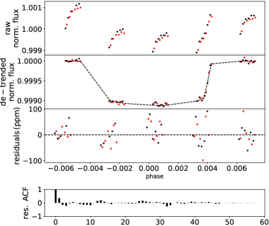
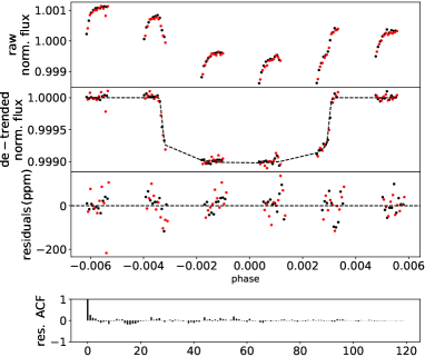
Figure 1: Results of the white light-curve analysis for the first considered transit of HD 106315 c (a) and the first considered transit of HD 3167 c (b). Top panel: normalized raw light-curve for the forward (black) and reverse (red) scans. Second panel: light-curves divided by the best-fit systematic effects model. Third panel: Fitting residuals. Bottom panel: auto-correlation function of residuals.

2.4 White light-curves fitting

The products of the previous steps are the white and spectral light-curves. To continue our characterization of the two exoplanet atmospheres we then created transmission spectra which were obtained by fitting the light-curves with a transit model. However, before fitting the extracted white and spectral light-curves, we had to consider the time-dependent systematics introduced by HST: one long-term ‘ramp’ (which affects all the visits) with a linear (and, in some cases, a quadratic) trend and one short-term ‘ramp’ (which affects every HST orbit) with an exponential trend.

In order to remove all these systematics, we fitted the white light-curves using the transit python package $PyLightcurve$, i.e. we used a transit model multiplied by a model for the systematics (Tsiaras et al., 2016b, 2018b):

where $t$ is time, $T_{0}$ is the mid-transit time, $t_{0}$ is the starting time of each HST orbit, $r_{a1}$ and $r_{a2}$ are the linear and quadratic systematic trend’s slope, $r_{b_{1}}$ and $r_{b_{2}}$ are the exponential systematic trend’s coefficients, and $n^{\mathrm{scan}}_{W}$ is a normalisation factor that changes for forward scanning ($n^{\mathrm{for}}_{W}$), and for reverse scanning ($n^{\mathrm{rev}}_{W}$). Second order (quadratic) visit-long ramps were also fitted for HD 3167 c visits because they were more affected by systematics. The parameter space was sampled via emcee (Foreman-Mackey et al., 2013). We used 300000 emcee iterations, 200 walkers, and 100000 burned iterations. We employed this set up for all the visits for both the planets. The only exception is represented by the fourth visit of HD 106315 c were we had to use 200000 iterations to obtain a good fit to our data.
Figure 1 shows the light-curves for the first transits of both exoplanets divided by the best-fit systematic model. (The same plots for the other transits are shown in appendix in Figure A.1). In the fit we took T₀ and R_P/R_⋆ as free parameters, and we used fixed values for $P$, $\omega$, $i$, $a/R_{\star}$, and $e$ parameters, as reported in Table 2. We made this choice because we miss ingress/egress observations in some visits. For both the planets we decided to eliminate data gathered during the first HST orbit and the first two points of each orbit because of the stronger systematics that affect them. An incorrect fitting of the behavior of the instrument at this stage would have introduced additional uncertainties in the final values of the transit parameters. Processing visits 3 and 4 for HD 3167 c required additional steps; this was on account of poor initial fitting due to HD 3167 b also transiting the stellar disk during these observations. Strong auto-correlation in the fit residuals for visits 3 and 4 led to an investigation of the orbits for both the transiting planets in the HD 3167 system: b and c. Theoretical transit light curves were plotted for all four HD 3167 observation windows, again using $PyLightcurve$ and taking parameters for both planets from Gandolfi et al. (2017). The theoretical light curves showed no overlap between transits for the first two visits but contamination of the third and fourth visits by concurrent transits of HD 3167 b. In both cases this effect was limited to a single HST orbit in each affected visit. These two orbits were then disregarded, leaving six orbits for each of visits 1, 2, and 5 five orbits apiece for vists 3 and 4. These affected orbits can be seen in the appendix in figure A.2. The final fitting results and their uncertainties can be found in Table 4.

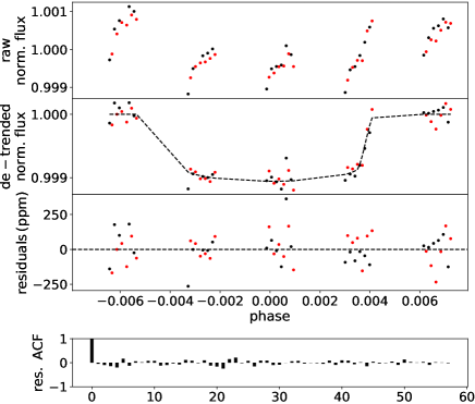
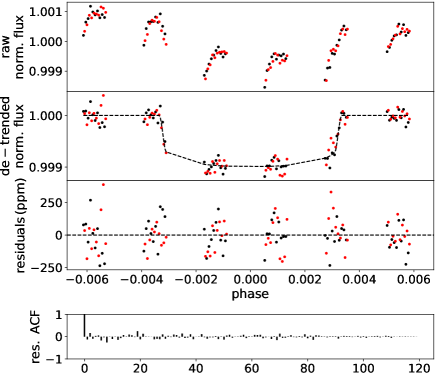
Figure 2: 10th bin ($\lambda\sim 1.3\;\upmu$m) spectral light-curve for the first transit of both HD 106315 c (a) and of HD 3167 c (b).

2.5 Spectral light-curves fitting

In order to correct for the systematics present in the spectral light-curves, we used the $divide$ $white$ $method$ introduced by Kreidberg et al. (2014c), i.e. each spectral light-curve was fitted with a model that includes the white light curve and its best-fit model:

$$\rm{n^{\mathrm{scan}}_{\lambda}\left[1-r_{a}(t-T_{0})\right]\frac{\mathrm{LC}_{W}}{\mathrm{M}_{W}}}$$ (2)

where $r_{a}$ is the coefficient of a wavelength-dependent linear slope along each HST visit, ${LC}_{W}$ is the white light-curve, ${M}_{W}$ is best fitting model to the white light-curve, $n^{\mathrm{scan}}_{\lambda}$ is the normalisation factor we used (it changes to $n^{\mathrm{for}}_{\lambda}$, when the scanning direction is upwards, and to $n^{\mathrm{rev}}_{\lambda}$ when it is downwards). As Table 4 shows we obtained big numbers for these normalization factors, these is due because the light curve are in units of electrons, thus the large values are reasonable. In the spectral light-curve fitting, the only free parameter is R_P/R_⋆, while the other parameters are the same as we used for the white light-curve fitting. Using the white light-curve as a comparison has the advantage that the residuals from fitting one of the spectral light-curves (see Figure 2) do not show trends similar to those in the white light-curve (see Figure 1). All the spectral and white light-curves we obtained, for the first HST visit of each planet, are plotted in Figure 3.

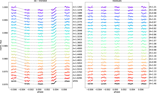
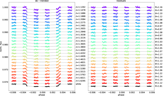
Figure 3: Analysis of the HD 106315 c (a) and HD 3167 c (b) white and spectral light-curves (left panels), for the first transit, plotted with an offset for clarity. Left panels: over-plotted white (black points) and spectral (coloured points) light-curves. Right panels: over-plotted residuals, $\bar{\sigma}$ indicates the ratio between the standard deviation of the residuals and the photon noise. The reason for some $\bar{\sigma}$ fall below 1 because of the small number of datapoints. Hence the measured standard deviation is not always representative of standard deviation of the underlaying distribution. These values are displayed as an indication for the goodness of fit, highlighting the differences between the different wavelengths and most importantly differences between the white light curve and spectral light curves.

As for the white light-curves fitting, the parameters space was sampled by using the emcee method. In this case we used 50000 emcee iterations, 100 walkers and 20000 burned iterations.
Starting from the spectral light-curves, the final spectra were extracted and combined from the spectral light-curves by computing the average of the transit spectra weighted by their respective uncertainties. First we subtracted each spectrum by the corresponding white light-curve depth, and then we computed the weighted average of all the transit observations. Finally, we added the weighted average of all white light-curves values to the averaged spectrum. The white light transit depths were consistent between transits, except for visit 3 for HD 3167 c (0.0291$\pm$0.0005 compared to the weighted mean 0.03058$\pm$0.00015). This is probably due to remaining systematics or to stellar activity. We obtained a final spectrum with an increased S/N ratio (Table 5, and Figure 4) which we then used for atmospheric retrieval.

Table 5: Transit depth (R_P/R${}_{\star})^{2}$ for the different wavelength channels, where R_P is the planetary radius, R_⋆ is the stellar radius, and $\lambda$, is the center value of each wavelength channel.

HD 106315 c
$\lambda$	(RP/R${}_{\star})^{2}$
$\mu$m	%
1.1263	0.1064$\pm$0.0027
1.1478	0.1098$\pm$0.0019
1.1686	0.1060$\pm$0.0018
1.1888	0.1065$\pm$0.0019
1.2084	0.1068$\pm$0.0017
1.2275	0.1063$\pm$0.0019
1.2465	0.1082$\pm$0.0019
1.2655	0.1029$\pm$0.0018
1.2848	0.1078$\pm$0.0019
1.3038	0.1046$\pm$0.0017
1.3226	0.1068$\pm$0.0018
1.3415	0.1080$\pm$0.0019
1.3605	0.1130$\pm$0.0018
1.3801	0.1096$\pm$0.0018
1.4000	0.1099$\pm$0.0017
1.4202	0.1086$\pm$0.0017
1.4406	0.1130$\pm$0.0017
1.4615	0.1126$\pm$0.0019
1.4831	0.1111$\pm$0.0019
1.5053	0.1116$\pm$0.0017
1.5280	0.1074$\pm$0.0019
1.5516	0.1106$\pm$0.0020
1.5762	0.1044$\pm$0.0019
1.6021	0.1062$\pm$0.0019
1.6295	0.1018$\pm$0.0020

HD 3167 c
$\lambda$	(RP/R${}_{\star})^{2}$
$\mu$m	%
1.1263	0.0950$\pm$0.0012
1.1478	0.0945$\pm$0.0012
1.1686	0.0926$\pm$0.0012
1.1888	0.0924$\pm$0.0011
1.2084	0.0930$\pm$0.0012
1.2275	0.0935$\pm$0.0011
1.2465	0.0909$\pm$0.0011
1.2655	0.0915$\pm$0.0011
1.2848	0.0903$\pm$0.0012
1.3038	0.0913$\pm$0.0011
1.3226	0.0912$\pm$0.0011
1.3415	0.0920$\pm$0.0011
1.3605	0.0928$\pm$0.0011
1.3801	0.0949$\pm$0.0011
1.4000	0.0955$\pm$0.0011
1.4202	0.0961$\pm$0.0011
1.4406	0.0970$\pm$0.0011
1.4615	0.0937$\pm$0.0011
1.4831	0.0958$\pm$0.0012
1.5053	0.0925$\pm$0.0012
1.5280	0.0944$\pm$0.0012
1.5516	0.0938$\pm$0.0012
1.5762	0.0957$\pm$0.0012
1.6021	0.0937$\pm$0.0012
1.6295	0.0932$\pm$0.0013

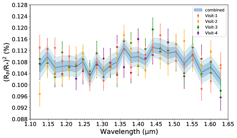
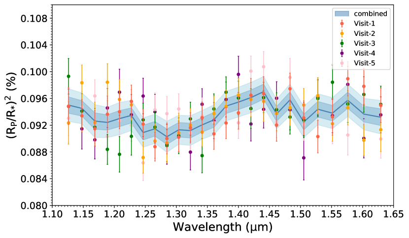
Figure 4: Spectra per visit and final weighted average with 1$\sigma$ and 2$\sigma$ uncertainty ranges for HD 106315 c (a) and HD 3167 c (b).

3 Atmospheric characterisation

Table 6: Fit evaluation criteria and maximum a-posteriors retrieval results.

Retrieved parameters bounds HD 106315 c HD 3167 c T_P (K) $\pm$60$\%$ T_eq 630${}^{+326}_{-115}$ 440${}^{+119}_{-79}$ R_P (R_J) $\pm$50$\%$ R_P 0.395${}^{+0.009}_{-0.021}$ 0.246${}^{+0.002}_{-0.002}$ log₁₀[H₂O] [-12 ; -1] $-2.1^{+0.7}_{-1.3}$ $-4.1^{+0.9}_{-0.9}$ log₁₀[NH₃] [-12 ; -1] $-4.3^{+0.7}_{-2.0}$ $<-5$ log₁₀[CO₂] [-12 ; -1] unconstrained $-2.4^{+0.7}_{-1.0}$ log₁₀[CO] [-12 ; -1] unconstrained unconstrained log₁₀[CH₄] [-12 ; -1] $<-5$ $<-5$ log₁₀[P_clouds/1Pa] [-2 ; 6] 3.7${}^{+1.4}_{-1.3}$ 5.3${}^{+0.5}_{-0.5}$ $\mu$ (derived) 2.38${}^{+0.52}_{-0.07}$ 2.44${}^{+0.66}_{-0.13}$ ADI - 15.97 9.58 $\Delta_{\rm E2}$ - 6.07 6.65 $\chi^{2}$ - 22.35 24.62 $\sigma$-level - 5.99$\sigma$ 4.76$\sigma$

3.1 TauREx setup

Once each planetary spectrum was obtained, we fitted it using the retrieval code TauREx3 (Al-Refaie et al., 2019). This algorithm uses the nested sampling code Multinest (Feroz et al., 2009) to map the atmospheric forward model parameter space and find the best fit to our empirical spectra. In our retrieval analysis we used 1500 live points and an evidence tolerance of 0.5.

The atmosphere of the two warm small planets was simulated by assuming an isothermal temperature-pressure (T/P) profile with molecular abundances constant as a function of altitude. These assumptions are acceptable since, due to the short wavelength covered by HST/WFC3, we are probing a restricted range of the planetary T/P profile (Tsiaras et al., 2018b). We note that this may not be the case anymore with next generation space telescopes (Rocchetto et al., 2016; Changeat et al., 2019). We calculated the equilibrium temperatures of the two planets using the following formula:

$$\rm T_{\rm{eq}}=\rm T_{\star}\left(\frac{\rm R_{\star}}{2\,a}\right)^{1/2}(1-\rm{A})^{1/4}$$ (3)

where $R_{\star}$ is the stellar radius, $a$ is the semi-major axis, $A$ is the geometric albedo. Assuming an albedo of 0.2 (Crossfield & Kreidberg, 2017), we obtained a temperature of $835\pm 20$ K and $518\pm 12$ K for HD 106315 c and HD 3167 c, respectively. We then used a wide range of temperature priors $\pm{60\%}$ $T_{\rm{eq}}$ ($334$–$1336$ K for HD 106315 c, and $207$–$829$ K for HD 3167 c) to allow different temperatures around the expected $T_{\mathrm{eq}}$. The planetary radius is also fitted in the model ranging from $\pm 50\%$ of the values reported in Table 2 (0.22-0.68 R_J for HD 106315 c, and 0.12-0.38 R_J for HD 3167 c).

We simulated atmospheres with pressures between $10^{-2}$ and $10^{6}$ Pa, uniformly distributed in log-space across 100 plane-parallel layers. We considered the following trace-gases: H₂O (Polyansky linelist, Polyansky et al., 2018), CH₄ (Exomol linelist, Yurchenko & Tennyson, 2014), CO (linelist from Li et al., 2015), CO₂ (Hitemp linelist, Rothman et al., 2010), NH₃ (Exomol linelist, Yurchenko et al., 2011) and assumed the atmosphere to be H₂/He dominated. Each trace-gas abundance was allowed to vary between $10^{-12}$ and $10^{-1}$ in volume mixing ratios (log-uniform prior). We used absorption cross-sections at a resolution of 15000 and include Rayleigh scattering and collision induced absorption of H₂–H₂ and H₂–He (Abel et al., 2011; Fletcher et al., 2018; Abel et al., 2012). Clouds are modeled assuming a grey opacity model and cloud top pressure bounds are set between $10^{-2}$ and $10^{6}$ Pa. All priors are listed in Table 6. Recently, Kreidberg et al. (2020) presented a transmission spectrum of HD 106315 c based on HST/WFC3, K2, and Spitzer observations. They chose to add N₂ in the retrieval analysis of HD 106315 c to compensate for invisible molecular opacities that could impact the mean molecular weight. The high equilibrium temperature of HD 106315 c ($\sim$800 K) suggests indeed the favored presence of N₂. However, we note that no further constraints have been found regarding N₂ opacity in the posterior distributions presented in Kreidberg et al. (2020) . Considering this result and for consistency with HD 3167 c whose equilibrium temperature is lower ($\sim$500 K), we decided to consider NH₃ instead of N₂ in the retrieval analysis for both planets. This choice is mainly motivated by the low density of HD 106315 c ($\sim$600 kg/m³) indicating, most likely, a primary light atmosphere. We therefore decided not to add N₂ to the analysis in order to maintain a primary mean molecular weight ($\mu\sim$2.3 amu).

To assign a significance to our detection, we used the ADI (Atmospheric Detectability Index) (Tsiaras et al., 2018b). It is a positively defined Bayes Factor between the nominal atmospheric model and a flat-line model (a model which contains no active trace gases, Rayleigh scattering or collision induced absorption). We also computed two other Bayes factors in the same way as the ADI. The first one, $\Delta_{\rm E1}$ is used to compute the significance of a molecule detection using a Bayes factor between the nominal atmospheric model and the same model without the considered molecule. The second one, $\Delta_{\rm E2}$ compares a given model to a model containing only water, Rayleigh scattering and collision-induced absorption as the reference Bayesian’s evidence. It is used to asses the necessity of a complex model to explain the atmosphere of the observed planet. These Bayes factors were then translated into a statistical significance (Kass & Raftery, 1995) by using Table 2 of Benneke & Seager (2013). Significances greater than 3.6 are considered ‘strong’, 2.7-3.6 are ‘moderate’, 2.1-2.7 ‘weak’, and below 2.1 ‘insignificant’.

3.2 Results

Table 6 lists our full TauREx retrieval results for the two planets while posterior distributions are plotted in Figure 7 and Figure 8. Retrieved best-fit spectra and corresponding best-fit molecular opacity contributions are shown in Figure 6. For each opacity source, the contribution function is the transit depth that we would obtain if the molecule was alone in the atmosphere. Therefore, the opacity sources, like H₂O in HD 3167 c (Figure 6 d) are never fully dominant since there are always some residuals CIA, Rayleigh or other molecules that contribute to the model. Opacity contributions are represented for one solution, the one considered as the best one statistically speaking, i.e with the highest log evidence. The offset opacities correspond to molecules that do not contribute to the fit and are found to be unconstrained. Besides, the grey line in Figure 6 c and d represents the top cloud pressure retrieved by TauREx for the best fit solution. The signal is theoretically blocked by this layer and nothing can be observed at higher pressures. Opacities found below this line are unconstrained. Using the Bayesian log evidences, we computed the ADI, $\Delta_{\rm E1}$ and $\Delta_{\rm E2}$ as explained in § 3.1. For both planets, retrieval results are consistent with water absorption features detectable in the spectral band covered by the G141 grism. We note a significant detection of carbon-bearing species in the atmosphere of HD 3167 c consistent with CO₂ absorption features. This result is unexpected, indeed, considering the planetary equilibrium temperature, CH₄ features are more likely to be present than CO₂ (see e.g., Figure 5 and Venot et al., 2020).

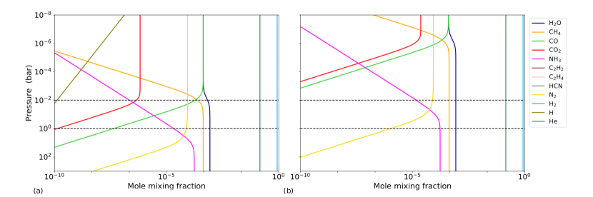
Figure 5: Thermochemical-equilibrium abundances for an atmosphere with an isothermal T/P profile and a temperature equal to that of HD 106315 c, T_eq=835.0 K, (a panel), and to that of HD 3167 c, T_eq=518.0 K, (b panel). These abundances’ profiles have been calculated using the Reliable Analytic Thermochemical Equilibrium (RATE) Python open-source package (Cubillos et al., 2019), assuming a solar elemental composition. Panel a highlights that given the range of pressures probed by HST/WFC3 -marked by black dashed horizontal lines-, and the planet’s equilibrium temperature the presence of N₂ should be favour over that of NH₃ in the atmosphere of HD 106315 c. Moreover, panel b shows as H₂O, CH₄, and NH₃ are the expected molecules in the atmosphere of HD 3167 c

.

Other species like NH₃, CO and CH₄ have either unconstrained or low abundances. They could be present in both atmospheres, but spectra do not present significant absorption features. We note however that NH₃ abundance is better constrained in the atmosphere of HD 106315 c (see Figure 7). Clouds top pressure is retrieved at different levels, $10^{3.7}$ Pa for HD 106315 c and $10^{5.3}$ Pa for HD 3167 c, corresponding to an upper bound (see the posterior distribution in Figure 7, and 8). The presence of molecular features in our spectra suggests a clear atmosphere for both planets. If opaque clouds are present, they are located below the region probed by WFC3/G141 observations.

(a)

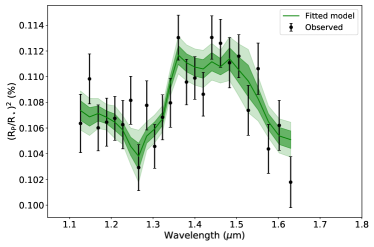
(b)

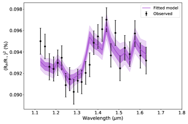
(c)

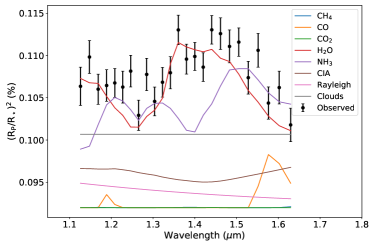
(d)

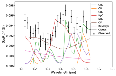
Figure 6: Best-fit atmospheric modeling results for HD 106315 c (a and c) and HD 3167 c (b and d).
Top panels: best fit spectra, 1$\sigma$ and 2$\sigma$ uncertainty ranges. Bottom panels: contributions of active trace gases, Rayleigh scattering, collision induced absorption (CIA), and clouds. From c and d panels it is evident that some opacity contributions are very offset from the data. These correspond to molecules that do not contribute to the fit and are found to be unconstrained.

3.2.1 HD 106315 c

According to the ADI, we retrieved a significant (5.99$\sigma$) atmosphere around the warm Neptune HD 106315 c with a notable water detection. H₂O is the only species that explains the absorption features between 1.3 and 1.5 $\rm{\mu}$m (Figure 6). We obtained a temperature of $630^{+326}_{-115}$ K which is lower than the equilibrium temperature, but consistent within 1$\sigma$. This could be explained by the fact that we are probing the atmosphere in the terminator area, and we modeled the atmosphere in 1D using an isothermal profile (Caldas et al., 2019; MacDonald et al., 2020; Pluriel et al., 2020a). Skaf et al. (2020), by analysing their three Hot Jupiters (WASP-127 b, WASP-79 b and WASP-62 b) together with the exoplanets from Tsiaras et al. (2018b), highlighted the existence of a global trend between the equilibrium and the retrieved temperatures, with the retrieved temperatures showing almost always lower values. In Figure 9 we updated Figure 6 from Skaf et al. (2020) by adding the retrieved/equilibrium temperatures of the two Neptunes-like planets analysed in this work. We can see that HD 106315 c follows the global trend.
The best-fit solution contains a notable amount of water, $\log_{10}[\mathrm{H_{2}O}]=-2.1^{+0.7}_{-1.3}$. Figure 7 shows that the right wing of the water’s abundance Gaussian distribution is not complete. This indicates that the abundance of H₂O could take even higher values ($\log_{10}[\mathrm{H_{2}O}]\sim-1$), but this is an unrealistic solution for a primary atmosphere, expected here for this Neptune-type planet. This is due to the limited coverage of HST/WFC3 G141. We note that the Bayes factor between a pure water model and the full chemical model $\Delta_{\rm E2}$ is equal to 6.07 (see Table 7) meaning that the complexity of the full chemical model is justified with a ‘strong’ significance (3.91$\sigma$).

The temperature retrieved by TauRex ($\sim$600 K) is compatible with absorption from NH₃, and this strenghtens our choice to consider NH₃ as active gas instead of N₂. However, NH₃ contribution is debatable – the detection is driven by a few points at 1.28, 1.55 $\rm{\mu}$m and 1.60 $\rm{\mu}$m, hence the weak abundance of $\log_{10}[\mathrm{NH_{3}}]=-4.3^{+0.7}_{-2.0}$. We note that a high temperature solution gives no constraint on NH₃ abundance whereas a lower temperature requires the molecule to be present (Figure 7). NH₃ abundance is also correlated to the amount of H₂O. Moreover, we can only put constraints on the higher abundance of CH₄: it could be found below $10^{-5}$. CO and CO₂ abundances are unconstrained. The model finds a clouds top pressure of $10^{3.7}$ Pa correlated to the amount of H₂O: the deeper the clouds are, the more water we have. The best-fit solution suggests a clear atmosphere with a significant amount of water. In order to give an estimation of the planetary C/O ratio, we employed the following formula re-adapted from MacDonald & Madhusudhan (2019): $C/O=(XCH_{4}+XCO+XCO_{2})/(XH_{2}O+XCO+2CO_{2})$, where the numerator indicates all species containing C atoms, while the numerator indicates all other O-bearing species. As we obtained a constrained value only for the water abundance, we decided to explore the range of valid C/O by using not only the mean abundances, but also the upper/lower possible values allowed by the posteriors (see Table 6). In this way, we obtained a C/O ratio that could vary in the range (7.5 $\times$10^-9-0.60).

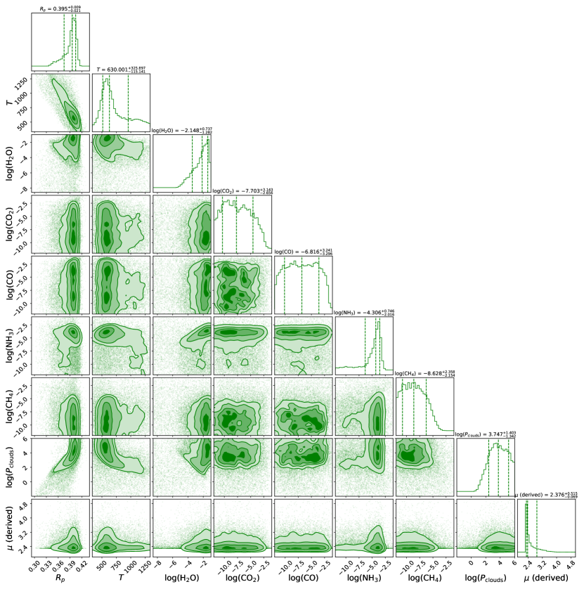
Figure 7: HD 106315 c atmospheric retrieval posterior distributions

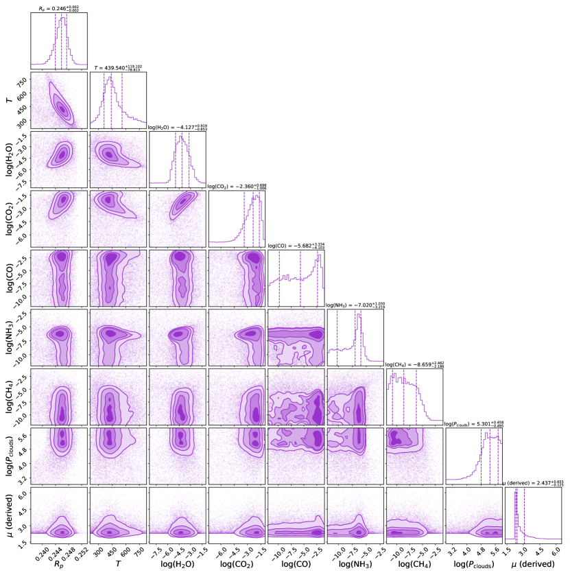
Figure 8: HD 3167 c atmospheric retrieval posterior distributions

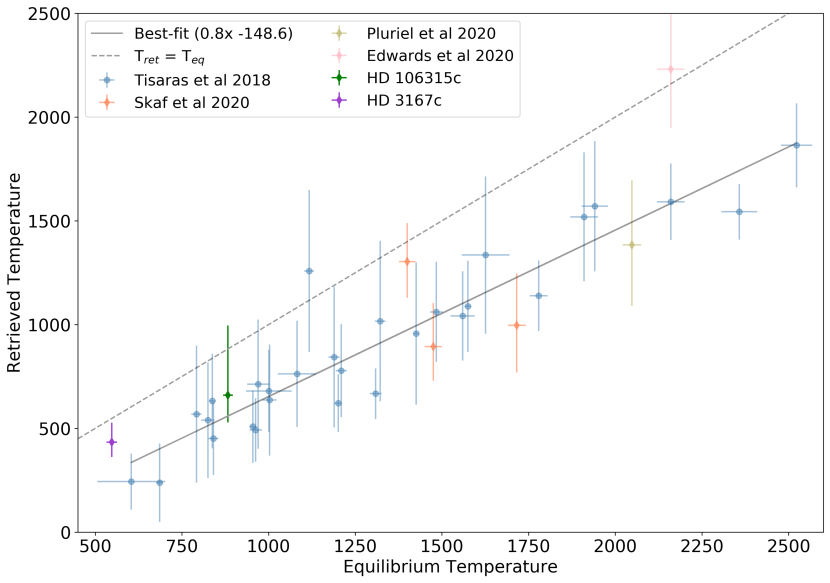
Figure 9: Trend between the retrieved and the equilibrium temperatures (or irradiation temperature) for the planets studied in Tsiaras et al. (2016b), Skaf et al. (2020), and the two planets analysed in this work. For consistency with the above-mentioned two works, a zero albedo has been assumed to calculate the equilibrium temperature. For completeness, the planets studied in ARES I (Edwards et al., 2020) and in ARES III (Pluriel et al., 2020b) are shown too.

3.2.2 HD 3167 c

The ADI value found for HD 3167 c retrieval is lower than the one computed for HD 106315 c (Table 6), yet it corresponds to a 4.76$\sigma$ significance detection of an atmosphere around this sub-Neptune. The temperature retrieved by TauREx ($440^{+119}_{-79}$ K) is lesser then the equilibrium temperature obtained assuming an albedo equal to 0.2, but it is consistent within 1$\sigma$.

The main difference with HD 106315 c’s atmosphere is the strong detection of CO₂, and more generally the presence of carbon-bearing species. Opacity source contributions in Figure 6 show both water and carbon dioxide features; these two species seem required to fit the data obtained by HST/WFC3 and their abundances are highly correlated (see Figure 8). $\Delta_{\rm E2}$ is equal to 6.65 (Table 7) meaning that the full chemical model is statistically significant (4.07$\sigma$) compared to a pure water model. This is probably driven by the carbon dioxide detection that explains the absorption features at $1.20\;\upmu$m, $1.45\;\upmu$m, and $1.60\;\upmu$m. The best-fit solution contains a significant amount of carbon dioxide $\log_{10}[\mathrm{CO_{2}}]=-2.4^{+0.7}_{-1.0}$ and a lower amount of water $\log_{10}[\mathrm{H_{2}O}]=-4.1^{+0.9}_{-0.9}$. As explained in § 3.2 we would have expected CH₄ to be the main carbon-bearing species instead of CO₂.

Looking at the posterior distributions in Figure 8, we can constrain the higher limits of ammonia and methane abundances, which are below $10^{-5}$. The monoxide abundance posterior distribution is highly degenerate, hence the weak detection. Carbon dioxide and monoxide features are difficult to distinguish in WFC3/G141 observations because they have similar features between $1.5\;\upmu$m and $1.6\;\upmu$m, leading potentially to degeneracies between the two abundances. The amounts of H₂O and CO₂, as well as the planet temperature and radius are correlated. For less water and carbon dioxide, the model requires a higher temperature and lower radius at $10$ bar atmospheric pressure (see Figure 8). The best-fit solution suggests a clear atmosphere with a top cloud pressure retrieved at $1$ bar. As for HD 106315 c, we derived a range of possible values in which the C/O ratio could vary, i.e. (0.49-0.85).

4 Discussion

Considering the narrow wavelength coverage and the low data resolution, the results obtained here are to be considered carefully and put into perspective. The model we tested has 8 free parameters and 25 observation data points. Molecular abundances and temperatures retrieved by TauREx are sensitive to the inputs and bounds set up by the users. TauREx gives us a first insight into these exoplanets’ atmospheres and, in particular for HST/WFC3, helps us to infer the presence of water. To better constrain the molecular detections found in § 3.2, we analysed different simulations (A0-A5 and B0-B7 in Table 7, for HD 106315 c and HD 3167 c, respectively) that include the expected molecules considering the wavelength coverage and the equilibrium temperature A0 and B0 are flat-line models that help us compute the ADI and A2 and B2, pure water models are used to compute $\Delta_{\rm E2}$.

Table 7: Comparison of the Bayesian log evidence for different models. The logarithm is taken to the base 10 (log $\rightarrow$ log₁₀).

HD 106315 c
N∘	Setup	Log E	ADI	$\Delta_{\rm E1}$	$\Delta_{\rm E2}$	T(K)	RP (RJ)	log[Pclouds/1Pa]	log[H2O]	log[NH3]	log[CH4]
A0	No active gas	210.94	N/A	N/A	N/A	$798^{+356}_{-315}$	0.388${}^{+0.027}_{-0.035}$	2.5${}^{+2.5}_{-3.2}$	N/A	N/A	N/A
A1	Full chemical	226.91	15.97	N/A	6.07	$630^{+326}_{-115}$	0.395${}^{+0.009}_{-0.021}$	$3.7^{+1.4}_{-1.3}$	$-2.1^{+0.7}_{-1.3}$	$-4.3^{+0.7}_{-2.0}$	$<-5$
A2	H2O only	220.84	9.52	N/A	N/A	$859^{+66}_{-99}$	0.404${}^{+0.002}_{-0.002}$	N/A	$-5.1^{+0.3}_{-0.2}$	N/A	N/A
A3	No H2O	212.70	1.76	14.21	N/A	$417^{+156}_{-56}$	$0.402^{+0.006}_{-0.011}$	$4.1^{+1.3}_{-1.8}$	N/A	$-3.4^{+1.0}_{-1.5}$	$-3.0^{+1.0}_{-2.9}$
A4	No clouds	226.98	16.04	N/A	6.14	$546^{+93}_{-87}$	$0.402^{+0.005}_{-0.007}$	N/A	$-2.1^{+0.7}_{-1.5}$	$-4.3^{+0.7}_{-1.0}$	$<-5$
A5	No NH3	226.00	15.06	0.91	5.16	$1004^{+223}_{-278}$	0.374${}^{+0.022}_{-0.020}$	$2.5^{+1.1}_{-0.9}$	$-2.6^{+1.1}_{-1.3}$	N/A	$<-5$
HD 3167 c
N∘	Setup	Log E	ADI	$\Delta_{\rm E1}$	$\Delta_{\rm E2}$	T(K)	RP (RJ)	log[Pclouds/1Pa]	log[H2O]	log[CO2]	log[CO]
B0	No active gas	225.84	N/A	N/A	N/A	$473^{+225}_{-180}$	0.238${}^{+0.010}_{-0.016}$	$2.2^{+2.6}_{-2.6}$	N/A	N/A	N/A
B1	Full chemical	235.41	9.58	N/A	6.65	$440^{+119}_{-79}$	0.246${}^{+0.002}_{-0.002}$	$5.3^{+0.5}_{-0.5}$	$-4.1^{+0.9}_{-0.9}$	$-2.4^{+0.7}_{-1.0}$	unconstrained
B2	H2O only	228.76	2.92	N/A	N/A	$785^{+33}_{-73}$	0.2425${}^{+0.0009}_{-0.0006}$	N/A	$-5.62^{+0.19}_{-0.18}$	N/A	N/A
B3	No H2O	231.80	5.97	3.61	N/A	$449^{+100}_{-88}$	0.246${}^{+0.002}_{-0.002}$	$5.1^{+0.6}_{-0.6}$	N/A	$-1.9^{+0.5}_{-0.8}$	unconstrained
B4	No clouds	236.45	10.62	N/A	7.69	$426^{+127}_{-75}$	0.246${}^{+0.002}_{-0.002}$	N/A	$-4.2^{+0.9}_{-0.8}$	$-2.4^{+0.7}_{-1.0}$	unconstrained
B5	No CO2	231.48	5.64	3.93	2.72	$605^{+151}_{-237}$	0.245${}^{+0.003}_{-0.003}$	$5.2^{+0.5}_{-0.7}$	$-4.8^{+1.4}_{-0.6}$	N/A	$-1.9^{+0.5}_{-1.6}$
B6	No CO	234.84	9.00	0.60	6.08	$440^{+110}_{-82}$	0.246${}^{+0.002}_{-0.002}$	$5.3^{+0.5}_{-0.6}$	$-3.9^{+1.1}_{-1.0}$	$-2.1^{+0.7}_{-0.9}$	N/A
B7	No CO2, CO	229.86	4.03	5.55	1.10	$732^{+60}_{-105}$	0.2423${}^{+0.0013}_{-0.0009}$	$5.4^{+0.4}_{-0.4}$	$-5.5^{+0.3}_{-0.2}$	N/A	N/A

4.1 Strength of H₂O detection

For both planets, to assess the significance of H₂O detection, we removed this active gas from the full chemical model and we analysed the Bayes factor $\Delta_{\rm E1}$. It decreases from 226.91 (A1) to 212.70 (A3) (see Table 7) and from 235.41 (B1) to 231.80 (B3) for HD 106315 c and HD 3167 c, respectively. H₂O detection is statistically confirmed for both planets with a ‘strong’ significance (5.68$\sigma$) for HD 106315 c, and a ‘moderate’ one (3.17$\sigma$) for HD 3167 c. In the recent paper by Kreidberg et al. (2020), they reported a tentative detection (with a Bayes factor of 1.7 or 2.6, depending on prior assumptions) of water vapor with a small amplitude of 30 ppm. In this simultaneous and independent analysis, by using different algorithms both for the extraction of the transmission spectrum from the WFC3 data (with Iraclis), and for the retrieval analysis (performed with TauREx3), we also detect the presence of water in the atmosphere of HD 106315 c with a high significance. Moreover our observed spectrum seems to be compatible with deeper H₂O features, which reinforces the detection. To date, water has been detected on several Neptune and sub-Neptune planets which allows comparisons. HD 106315 c could be compared to to HAT-P-11 b (with a water detection’s significance, hereafter $\sigma_{\rm{H_{2}O}}$, of 5.1$\sigma$, Fraine et al. 2014), and to GJ 3470 b ($\sigma_{\rm{H_{2}O}}$= 5.2$\sigma$, Benneke et al. 2019a). While HD 3167 c has a lower water detection, appearing more similar to K2-18 b ($\sigma_{\rm{H_{2}O}}$=3.6$\sigma$, Tsiaras et al. 2019, and $\sigma_{\rm{H_{2}O}}$=3.93$\sigma$, Benneke et al. 2019b). Crossfield & Kreidberg (2017) studied the water features amplitude of six warm Neptune planets and highlighted correlations with the equilibrium temperature and the mass fraction of hydrogen and helium. To verify the correlation of H₂O amplitude, in units of atmospheric scale height, with the equilibrium temperature we computed HD 106315 c, HD 3167 c and K2-18 b water amplitude using HST/WFC3 spectra obtained here and in Tsiaras et al. (2019). We used the same method described in Crossfield & Kreidberg (2017). We fitted a carbon-free template of GJ 1214 b normalized in units of scale height (Crossfield et al., 2011) to the observations using the Levenberg and Marquardt’s least squares method (L-M) (Markwardt, 2009). Then, we measured the amplitude taking the normalized average value from 1.34${\rm\mu}$m to 1.49${\rm\mu}$m and subtracting it from the average value outside this wavelength range. The scale height H=K_BT_eq/${\rm\mu}$g is computed assuming a hydrogen rich atmosphere (${\rm\mu}$=2.3 amu) and the equilibrium temperature is calculated for an albedo of 0.2. We find a water feature amplitude of 1.02$\pm$0.18 for HD 106315 c, of 1.04$\pm$0.24 for HD 3167 c, and of 1.28$\pm$0.49 for K2-18 b. We note that Kreidberg et al. (2020) recent paper found a lower absorption feature, i.e 0.80$\pm$0.04 for HD 106315 c. We plot our values in Figure 10 along with the amplitudes computed in Crossfield & Kreidberg (2017) and the ones found in Libby-Roberts et al. (2020) for Kepler 51 b and Kepler 51 d. Finally, we fitted a linear relation and compared the Pearson correlation coefficient and the probability. We find a correlation coefficient of 0.43 and a p-value of 0.18. The strong correlation highlighted in Crossfield & Kreidberg (2017) is not found here, mostly because of K2-18 b high water feature amplitude at low temperature. While removing K2-18 b and Kepler 51 d amplitudes – to focus on planets with temperature between 500 and 1000 K as in Crossfield & Kreidberg (2017)- we find a correlation coefficient of 0.70 and p-value of 0.04 while they found a coefficient of 0.83 for a p-value equal to 0.04. A refinement of the scale height, HST/WFC3 water amplitude and correlations computations will be detailed in a follow-up paper focusing on intermediate size planets (R${}_{\rm P}<$ 6 R_⊕) with consistent published spectra.

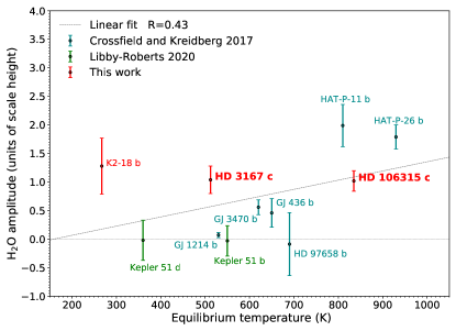
Figure 10: Normalized H₂O amplitude in units of scale height with respect to equilibrium temperatures. Blue points are from Crossfield & Kreidberg (2017) and green points are from Libby-Roberts et al. (2020). Red points are computed using the method described in Crossfield & Kreidberg (2017) and spectra obtained in this work and from Tsiaras et al. (2019) for K2-18 b. The dotted line corresponds to a linear fit. The correlation coefficient was found to be lower than in Crossfield & Kreidberg (2017), 0.43 compared to 0.83.

4.2 Clear or cloudy atmospheres

In § 3.2, we retrieved a clear atmosphere for both planets, but we expect species to condense and clouds to form on warm Neptune and sub-Neptune planets. The flat spectra of GJ 436 b (Knutson et al., 2014a), GJ 1214 b (Kreidberg et al., 2014b) and HD 97658 b (Knutson et al., 2014b) were interpreted as high cloud or haze at low pressure. We confirm the clear atmosphere by removing the cloud top pressure parameter from the full chemical model. ADIs of cloud free models (A4 and B4 in Table 7) are higher than ADIs of full chemical models including clouds (A1 and B1 in Table 7). Clouds do not impact retrieval results, even for HD 106315 c with a lower top clouds pressure, and this means that either the planet has a clear atmosphere or the clouds are located below the visible pressure where the atmosphere is opaque. Looking at HD 106315 c’s clouds top pressure correlations with H₂O abundance (see Figure 7), a second mode appears meaning that clouds could be present in the region we are probing.

The TauREx retrieval does not bring any information on cloud composition and we must recall that the wavelength coverage is not wide enough to constrain cloud chemistry. All things considered, models have predicted that for hot atmospheres (900 to 1300 K) we could find condensates like KCl, ZnS and Na₂S, and for colder atmospheres (400 to 600 K) KCl and NH₄H₂PO₄ (Lodders & Fegley, 2006; Morley et al., 2012). GJ 1214 b (6.26 $\pm$ 0.86 M_⊕, 2.85 $\pm$ 0.20 R_⊕, Harpsøe et al. 2013), K2-18 b (8.92 $\pm$ 1.7 M_⊕, 2.37 $\pm$ 0.22 R_⊕, Sarkis et al. 2018 ) and HD 3167 c (this paper) have a similar mass and radius, and yet present very different atmospheric properties. The equilibrium temperature is lower for K2-18 b (284$\pm$15 K, Sarkis et al., 2018), but presents water detection. GJ 1214 b has a similar equilibrium temperature (547${}_{-8}^{+7}$, Kundurthy et al., 2011), but exhibits a flat spectrum suggesting the presence of clouds.

4.3 NH₃ in HD 106315 c’s atmosphere

HD 106315 c’s best fit solution includes a small amount of NH3, i.e $\log_{10}[\mathrm{NH_{3}}]=-4.3^{+0.7}_{-2.0}$. Looking at the posteriors distribution (Figure 7), NH₃ abundance converges toward a solution. To confirm this detection, we removed this gas from the full chemical model and computed $\Delta_{\rm E1}$ (see A5 in Table 7). The difference is 0.91 meaning that NH₃’s detection has to be considered ‘not-significant’ (1.97$\sigma$). However, we observe some differences, the temperature rises to 1004 K with less constraints and consequently, the radius decreases to 0.374 R_J. Clouds are found at a higher level $10^{2.5}$ Pa. The cloud deck compensates for NH₃ features by cutting H₂O ones and shrinking the spectrum. From this analysis, we conclude that HD 106315 c can be surrounded by either a primary clear atmosphere with H₂O and traces of NH₃ or by a primary atmosphere with H₂O and deep clouds.
As mentioned in § 3.1 the high equilibrium temperature of HD 106315 c should have favor the presence of N₂ instead of NH₃ (see e.g., Figure 5). NH₃ is expected to disappear above 500-550 K. However, we retrieve at the terminator, so we should expect a lower temperature (closer to this 500 K limit) and more NH₃. Moreover, N₂ is an inactive gas, with no feature in WFC3, which means that the ‘free’ retrieval we perform – the retrieval in ‘free’ mode is used to retrieve the abundance for active molecules that have features in the spectrum- will not pick up this molecule except if it influences the mean molecular weight. To test this, we added N₂ in the analysis to see the possible consequences that this molecule could have had on the mean molecular weight. We assumed an initial N₂ abundance of 10^-4, compatible with the one expected by thermochemical-equilibrium condition (see Figure 5), and we allowed it to vary between $10^{-12}$ and $10^{-1}$ in volume mixing ratios (log-uniform prior) -as for the other molecules. The inclusion of N₂ does not affect the mean molecular weight, a simple clouds model added to H₂O and NH₃ features are enough to fit the spectrum, there is no need to add extra molecular weight to shrink the spectrum. Moreover, NH₃ detection remains around 10^-4 (see Figure A.3).

4.4 CO₂ in HD 3167 c’s atmosphere

HD 3167 c best fit solution includes an important amount of CO₂ (i.e $\log_{10}[\mathrm{CO_{2}}]=-2.4^{+0.7}_{-1.0}$). This detection is supported by the data points from $\sim$1.5 to 1.6 $\mu$m, but water seems to explains better the absorption features around 1.4 $\mu$m (see Figure 6). We removed CO₂ from the full chemical and compared log evidences, it decreases from 235.41 (B1, Table 7 ) to 231.48 (B5) corresponding to a 3.28$\sigma$ “moderate” detection. The ADI decreases as well to 5.64. We note that CO is now compensating for CO₂ features and its log abundance increases to $\log_{10}[\mathrm{CO}]=-1.9^{+0.5}_{-1.6}$. This value is too high for a realistic primary hydrogen-rich atmosphere that we expect for this planet. We successively removed CO from the full chemical model, but it does not impact the retrieval results (B6 in Table 7) and $\Delta_{\rm E1}$ is below 1 (‘not significant’). Finally, we removed both CO and CO₂ to asses the detection of those carbon-bearing species (B7). The difference in log evidences is now equal to $\Delta_{\rm E1}$=5.55 and corresponds to more than 3$\sigma$ carbon detection. This test does not impact the abundance of water nor the top cloud pressure, but constrains better the abundance of ammonia to $10^{-6.4}$. We note that CH₄ does not compensate the lack of the other carbon-bearing species, it’s abundance remains constrained below $10^{-5}$. The temperature increases to keep a primary atmosphere hypothesis and an extended clear atmosphere.

This unexpected detection of carbon bearing species could be explained by noise or systematic effects that were not removed during the white light curve fitting step (see Section 2.4). It could also be the result of phenomena that our 1D equilibrium chemistry modeling cannot reproduce, e.g. 3D transport cross-terminator. An other interpretation could be the actual presence of CO₂ in the atmosphere of HD 3167 c due for example to a very high metallicity, enhanced over that of the host star which is consistent with solar metallicity ([Fe/H]=0.03$\pm$0.03 dex, Gandolfi et al. 2017). It is known indeed that the abundance of CO₂ scales quadratically with metallicity (see e.g. Moses, 2014), and other examples of overabundance of CO₂ interpreted as caused by an high metallicity can be found in the literature (see e.g. Madhusudhan & Seager, 2011). However, if we use the water abundance as a proxy of metallicity (see e.g., Kreidberg et al., 2014a) we infer a solar or sub-solar metallicity for HD 3167 c, which would be in tension with the possibility that CO₂ could be present due to high metallicity. More observations are thus necessary to better constraint a possible presence of CO₂ in the atmosphere of HD 3167 c.

4.5 Inferences from the Mass and Radius

There is a strong degeneracy in exoplanet interiors as there are many compositional models that are compatible with an observed mass and radius. However, by combining the mass, radius, and the spectroscopic results of our study we can get an inference for the interior composition of HD 106315 c and HD 3167 c. Our discovery of icy constituents, such as $\rm H_{2}O$ in both planetary atmospheres (and maybe $\rm NH_{3}$ in the envelope of HD 106315 c) indicate an ice-rich embryo. Curiously, the mass and radius of HD 106315 c and HD 3167 c are also consistent with an ice-rich core which we explain below.

For the following results we adopted the planetary models from Zeng & Sasselov (2013), Zeng et al. (2016), and Zeng et al. (2019b). Based on the mass and radius of HD 106315 c and HD 3167 c they are both consistent with icy cores with hydrogen envelopes $\sim 5~{}\rm wt.\%$ and $0.3-1~{}\rm wt.\%$ of their total planetary masses respectively. We show these results in Figure 11. Nevertheless, there is still enough uncertainty in the results that a silicate embryo engulfed by a hydrogen atmosphere is still plausible for both planets. Certainly, with improved mass and radius measurements, together with more accurate spectroscopic observations, the interior structure of exoplanets such as HD 106315 c and HD 3167 c will get further constrained. We discuss the implications of this in § 4.7.

Besides, Mousis et al. (2020) recent publication, showed that close-in planets could have water-rich hydrospheres in super-critical state. Their model suggests that intermediate-size planets could be hydrogen/helium-free and their interiors would simply vary from one another depending on the water content.

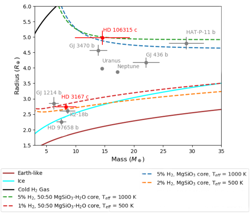
Figure 11: The mass and radius of HD 106315 c and HD 3167 c (from Table 2) plotted against other planets with size between 1.5-4 R_⊕ and published atmospheric characterization studies (see Table 1) -GJ 3470 b (Awiphan et al., 2016), GJ 436 b (Maciejewski et al., 2014), GJ 1214 b (Harpsøe et al., 2013), HD 97658 b (Van Grootel et al., 2014), HAT-P-11 b (Stassun et al., 2017), K2-18 b (Benneke et al., 2019b)- and Uranus and Neptune (https://nssdc.gsfc.nasa.gov/planetary/factsheet/). The mass and radius models are from Zeng & Sasselov (2013) and Zeng et al. (2016).

4.6 Comparison with previous results

This paper is the result of work carried out during the ARES Summer School, where we used algorithms and data available to the public, thus allowing our results to be tested and reproduced. This is the fourth paper output of this summer school. In the first work ARES I (Edwards et al., 2020) and in the third one ARES III (Pluriel et al., 2020b) we analysed the transmission and the emission spectra of WASP-76 b and Kelt-7 b respectively, while in the second one ARES II (Skaf et al., 2020), the atmospheric study of WASP-42 b, WASP-79 b, and WASP-127 b was performed. In this work, we used the ADI as a significance index to make the approach in our work uniform with these previous papers, with Tsiaras et al. (2018b), and with Tsiaras et al. (2019). Figure 12, shows the gaseous exoplanets studied by Tsiaras et al. (2018b) (in black), K2-18b examined in Tsiaras et al. (2019) (in blue), the hot Jupiters analysed in ARES I, ARES II, ARES III - for consistency with other works here we plot the ADI obtained from the analysis of WASP-76 b’s and Kelt-7 b’s transmission spectra - (in red), and finally the Neptune-like planets, HD 106315 c (in green) and HD 3167 c (in violet), studied in this paper. From this figure, it emerges that, even if the two exoplanets characterized in this paper have smaller radii than most of the other targets, their ADI is not smaller. Our study, together with Tsiaras et al. (2019), shows that even smaller planets’ atmospheres can be characterized with high significance. This opens the way for the atmospheric study of planets with smaller radii than the hot Jupiter targets which have mostly been analyzed so far.

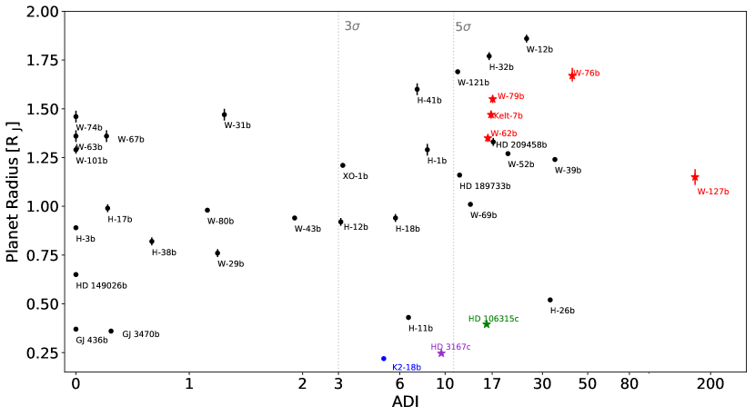
Figure 12: Exoplanetary radii as a function of the ADI index (in logarithmic scale) for the targets analysed in this work (in green and in violet), in ARES I-II-III (in red), in Tsiaras et al. (2016b) (in black), and in Tsiaras et al. (2019) (in blue).

4.7 Future Characterization

(a)

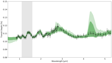
(b)

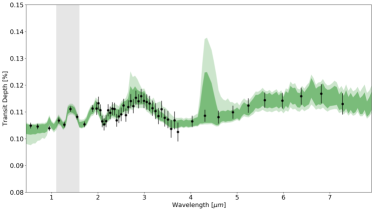
(c)

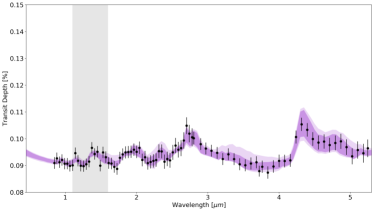
(d)

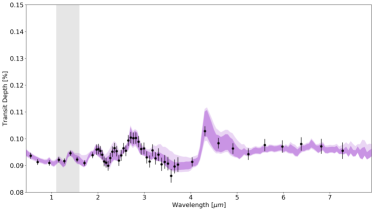
Figure 13: Simulated JWST (a and c) and Ariel (b and d) observations of the best-fit solutions, i.e. the full chemical scenario, retrieved in this work. For Ariel, 10 transits have been assumed for each planet, while JWST simulations have been performed using a single transit with NIRISS GR700XD as well as an observation with NIRSpec G395H. HD 106315 c and HD 3167 c are shown in green (a and b) and in purple (c and d), respectively.

It is evident that in the future the exoplanetary field will be based on the detailed characterisation of exo-atmospheres. In this scenario, NASA’s upcoming JWST telescope will play an important role; its large aperture, high sensitivity and wide spectral range will allow the detection of molecular species in the atmospheres of planets with different masses: from super Earths to super-Jovians. Scheduled to launch in the late 2020s, the ESA Ariel space mission will enable atmospheric characterisation of a large sample ($\sim$1000) of exoplanets in order to address how the chemical composition of an exoplanet is linked to its formation/evolution environment (Tinetti et al., 2018; Edwards et al., 2019a). With this prospect in mind, HD 106315 c and HD 3167 c represent suitable targets for both these space-borne instruments and so we used the Ariel Radiometric Model (ArielRad) (Mugnai et al., 2020) to simulate observations by Ariel. For each planet, we took the best-fit solution from the HST/WFC3 analysis to model Ariel observations at its native resolution (i.e. the TIER 3 resolution); we considered ten Ariel transits. In addition, we simulated JWST observations using ExoWebb Edwards et al. (2020), assuming the collection of one single transit using NIRISS GR700XD plus a transit with NIRSpec G395M. Figure 13, shows, for the two planets, the results of our simulations for both JWST (left panels, a and c) and Ariel (right panels, b and d). It highlights the increased wavelength coverage and data quality that will be obtained with both Ariel and JWST. The power of having a broad wavelength coverage is that we can probe multiple absorption bands for each molecule. This helps break degeneracies due to overlapping features and always molecular compositions to be more readily constrained. Additionally, these future missions could shore up the detections of both NH₃ (for HD 106315 c), and CO₂ (for HD 3167 c): the larger the spectral range covered, the more absorption bands may be present. Namely, on one hand, JWST and Ariel could highlights the CO₂ absorption features between $\sim$1.7-2.0 $\mu$m and 4.0-5.32 $\mu$m; on the other hand NH₃ presents strong absorption features at longer wavelengths compared to the one probed with WFC3.

5 Summary and conclusion

We presented here the analysis of HST/WFC3 spatially scanned observations of the Neptune-type HD 106315 c, and of the sub-Neptune HD 3167 c resulting in the detection of water vapor in both atmospheres. Starting from the raw data, and using the routine Iraclis, we extracted a transmission spectrum for both planets. We then interpreted it through the use of the Bayesian spectral retrieval algorithm TauREx3. We found a statistically significant atmosphere surrounding the two planets and evaluated the strength of our detection through the ADI metric.

From the TauREx analysis, we retrieved a ‘strong’ detection of H₂O ($\log_{10}[\mathrm{H_{2}O}]=-2.1^{+0.7}_{-1.3}$, $\Delta_{\rm E1}$=14.21) and a ‘possible evidence’ of NH₃ ($\log_{10}[\mathrm{NH_{3}}]=-4.3^{+0.7}_{-2.0}$, $\Delta_{\rm E1}$=0.91, even if it is not significant) in the atmosphere of HD 106315 c. When removing ammonia, a deep cloud deck is required to fit the spectrum. We can only put an upper bound on methane abundance ($10^{-5}$), while carbon dioxide and monoxide abundances are unconstrained.

The HD 3167 c analysis resulted in both a water vapor ($\log_{10}[\mathrm{H_{2}O}]=-4.1^{+0.9}_{-0.9}$, $\Delta_{\rm E1}$=3.61) and a carbon dioxide ($\log_{10}[\mathrm{CO_{2}}]=-2.4^{+0.7}_{-1.0}$, $\Delta_{\rm E1}$=3.93) ‘moderate’ detection. As CO₂ is not explained by 1D equilibrium chemistry models, its presence could be due to noise and highlights the limitations of our data quality. More precise constraints on the chemical abundances could be given if 3D models were employed instead of 1D ones. The shortcomings of retrieval analyses performed with 1D forward models have been highlighted already in previous papers (see e.g. Caldas et al., 2019). On the contrary, if we assume a high metallicity, CO₂ could actually be present in the atmosphere of HD 3167 c (an increase in metallicity by a factor of x tends to increase the abundance of CO₂ by a factor of x², see Moses 2014, see e.g.), and what we are seeing could not be due to noise or to systematics. Thus, further observations are needed to establish whether the CO₂ might actually be present in the atmosphere of this exoplanet.

The future is bright for atmospheric studies of exoplanets thanks to both space-based and ground-based facilities. On one hand, Cowan et al. (2015), Greene et al. (2016), Tinetti et al. (2018), and Edwards et al. (2019b) have shown the potential of the JWST, Twinkle, and Ariel space missions to characterize exo-atmospheres. On the other, ground-based instruments such as the European Extremely Large Telescope (E-ELT), -and in particular the Mid-Infrared E-ELT Imager and Spectrograph (METIS) instrument (Brandl et al., 2018)-, the Thirty Meter Telescope (TMT, Skidmore et al. 2018), and the Giant Magellan Telescope (GMT, Fanson et al. 2018), will become available. This will lead to the systematic study of thousands of exoplanets’ day sides and terminators both at high-(HRS, from the ground) and at low-(LRS, from the space) spectral resolution. By combining HRS with LRS, and thus probing different regions of the exoplanetary atmospheres (higher atmospheric altitudes with HRS, lower atmospheric altitudes with LRS), we will better understand the atmospheric compositions, and thus be able to apply more constraints on their formation and evolution. Given the brightness of their respective host stars, and the large scale heights we computed (H$\sim$518 $\pm$ 174 km and H$\sim$171 $\pm$ 40 km for HD 106315 c and HD 3167 c, respectively), the two Neptune-like planets we studied in this paper are suitable targets for these upcoming instruments.

Acknowledgments: We want to thank the anonymous referee for the constructive comments which helped improve the quality of the manuscript. This work was realised as part of “ARES Ariel School” in Biarritz in 2019. The school was organised by JPB, AT and IW with the financial support of CNES. JPB acknowledge the support of the University of Tasmania through the UTAS Foundation and the endowed Warren Chair in Astronomy, Rodolphe Cledassou, Pascale Danto and Michel Viso (CNES). WP, TZ, and AYJ have received funding from the European Research Council (ERC) under the European Union’s Horizon 2020 research and innovation programme (grant agreement n^∘ 679030/WHIPLASH and n^∘ 758892/ExoAI). SW was supported through the STFC UCL CDT in Data Intensive Science (grant number ST/P006736/1). GG acknowledges the financial support of the 2017 PhD fellowship programme of INAF. RB is a PhD fellow of the Research Foundation – Flanders (FWO). DB acknowledges financial support from the ANR project ”e-PYTHEAS” (ANR-16-CE31-0005-01). LVM and DMG acknowledge the financial support of the Ariel ASI grant n. 2018-22-HH.0. BE, QC, MM, AT and IW acknowledge funding from the European Research Council (ERC) under the European Union’s Horizon 2020 research and innovation programme grant ExoAI (GA No. 758892) and the STFC grants ST/P000282/1, ST/P002153/1, ST/S002634/1 and ST/T001836/1. NS acknowledges the support of the IRIS-OCAV, PSL. MP acknowledges support by the European Research Council under Grant Agreement ATMO 757858 and by the CNES. OV thank the CNRS/INSU Programme National de Planétologie (PNP) and CNES for funding support.

Appendix A Additional Figures

In this appendix section, in Figure A.1 we show the results of the white light-curve analysis for the transits not reported in Figure 1 for both the two exoplanets analysed in this work, whilst in Figure A.2 we plot the HD 3167 c’s orbits that showed contamination from HD 3167 b. The last Figure of the appendix (Figure A.3) shows the posterior distribution we obtained by including also N₂ in the retrieval analysis of HD 106315 c.

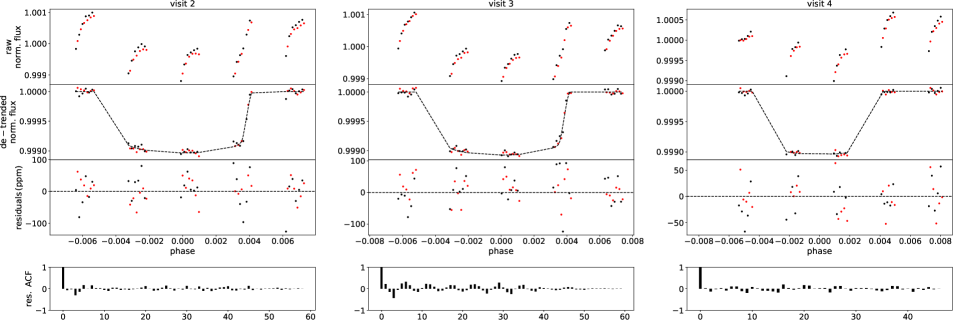
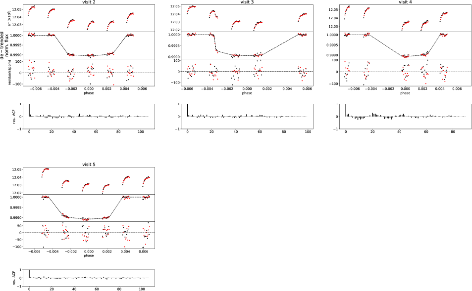
Figure A.1: Same as Figure 1 for the other transits both for HD 106315 c (a panels) and for HD 3167 c (b panels).

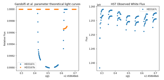
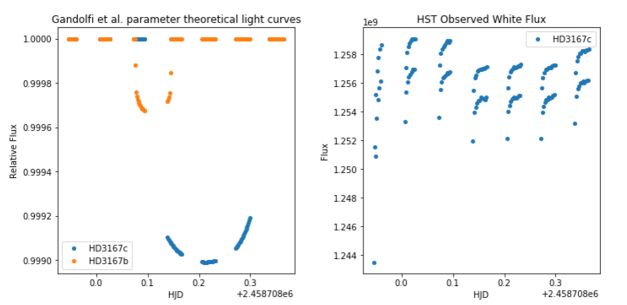
Figure A.2: HD 3167 c’s orbits that showed contamination from HD 3167 b. Visit 3 and the impact on its sixth orbit is shown in a), while visit 4 and the contamination of its third orbit is plotted in b).

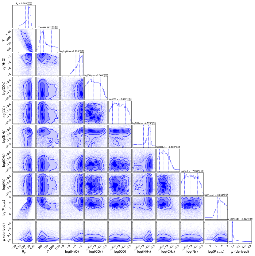
Figure A.3: HD 106315 c’s posterior distribution including also N₂ to the full chemical scenario. As this Figure shows, the inclusion of nitrogen does not affect the mean molecular weight. Moreover, the detection of NH₃ remains around 10^-4.

References

- Abel et al. (2011) Abel, M., Frommhold, L., Li, X., & Hunt, K. L. 2011, The Journal of Physical Chemistry A, 115, 6805
- Abel et al. (2012) —. 2012, The Journal of chemical physics, 136, 044319
- Al-Refaie et al. (2019) Al-Refaie, A. F., Changeat, Q., Waldmann, I. P., & Tinetti, G. 2019, arXiv e-prints, arXiv:1912.07759
- Allart et al. (2018) Allart, R., Bourrier, V., Lovis, C., et al. 2018, arXiv e-prints, arXiv:1812.02189 [astro-ph.EP]
- Astropy Collaboration et al. (2018) Astropy Collaboration, Price-Whelan, A. M., Sipőcz, B. M., et al. 2018, AJ, 156, 123
- Awiphan et al. (2016) Awiphan, S., Kerins, E., Pichadee, S., et al. 2016, MNRAS, 463, 2574
- Barros et al. (2017) Barros, S. C. C., Gosselin, H., Lillo-Box, J., et al. 2017, A&A, 608, A25
- Batalha et al. (2013) Batalha, N. M., Rowe, J. F., Bryson, S. T., et al. 2013, ApJS, 204, 24
- Benneke & Seager (2013) Benneke, B., & Seager, S. 2013, ApJ, 778, 153
- Benneke et al. (2019a) Benneke, B., Knutson, H. A., Lothringer, J., et al. 2019a, Nature Astronomy, 3, 813
- Benneke et al. (2019b) Benneke, B., Wong, I., Piaulet, C., et al. 2019b, ApJ, 887, L14
- Borucki et al. (2011) Borucki, W. J., Koch, D. G., Basri, G., et al. 2011, ApJ, 736, 19
- Bourrier et al. (2016) Bourrier, V., Lecavelier des Etangs, A., Ehrenreich, D., Tanaka, Y. A., & Vidotto, A. A. 2016, A&A, 591, A121
- Bourrier et al. (2018) Bourrier, V., Lecavelier des Etangs, A., Ehrenreich, D., et al. 2018, A&A, 620, A147
- Brandl et al. (2018) Brandl, B. R., Absil, O., Agócs, T., et al. 2018, in Society of Photo-Optical Instrumentation Engineers (SPIE) Conference Series, Vol. 10702, Proc. SPIE, 107021U
- Brown et al. (2001) Brown, T. M., Charbonneau, D., Gilliland, R. L., Noyes, R. W., & Burrows, A. 2001, ApJ, 552, 699
- Caldas et al. (2019) Caldas, A., Leconte, J., Selsis, F., et al. 2019, A&A, 623, A161
- Chachan et al. (2019) Chachan, Y., Knutson, H. A., Gao, P., et al. 2019, The Astronomical Journal, 158, 244
- Changeat et al. (2019) Changeat, Q., Edwards, B., Waldmann, I. P., & Tinetti, G. 2019, The Astrophysical Journal, 886, 39
- Christiansen et al. (2017) Christiansen, J. L., Vanderburg, A., Burt, J., et al. 2017, AJ, 154, 122
- Claret (2000) Claret, A. 2000, A&A, 363, 1081
- Collette (2013) Collette, A. 2013, Python and HDF5 (O’Reilly)
- Cowan et al. (2015) Cowan, N. B., Greene, T., Angerhausen, D., et al. 2015, Astrophysics - Earth and Planetary Astrophysics, 127, 311
- Crossfield et al. (2011) Crossfield, I. J. M., Barman, T., & Hansen, B. M. S. 2011, ApJ, 736, 17
- Crossfield & Kreidberg (2017) Crossfield, I. J. M., & Kreidberg, L. 2017, AJ, 154, 6
- Crossfield et al. (2017) Crossfield, I. J. M., Ciardi, D. R., Isaacson, H., et al. 2017, AJ, 153, 255
- Cubillos et al. (2019) Cubillos, P. E., Blecic, J., & Dobbs-Dixon, I. 2019, ApJ, 872, 111
- Díaz et al. (2014) Díaz, R. F., Almenara, J. M., Santerne, A., et al. 2014, MNRAS, 441, 983
- Dressing & Charbonneau (2013) Dressing, C. D., & Charbonneau, D. 2013, ApJ, 767, 95
- Edwards et al. (2020) Edwards, B., Al-Refaie, A., Lagage, P., & Gastaud, R. 2020, in prep
- Edwards et al. (2019a) Edwards, B., Mugnai, L., Tinetti, G., Pascale, E., & Sarkar, S. 2019a, AJ, 157, 242
- Edwards et al. (2019b) Edwards, B., Rice, M., Zingales, T., et al. 2019b, Experimental Astronomy, 47, 29
- Edwards et al. (2020) Edwards, B., Changeat, Q., Baeyens, R., et al. 2020, AJ, 160, 8
- Fanson et al. (2018) Fanson, J., McCarthy, P. J., Bernstein, R., et al. 2018, in Society of Photo-Optical Instrumentation Engineers (SPIE) Conference Series, Vol. 10700, Proc. SPIE, 1070012
- Feroz et al. (2009) Feroz, F., Hobson, M. P., & Bridges, M. 2009, MNRAS, 398, 1601
- Fisher & Heng (2018) Fisher, C., & Heng, K. 2018, MNRAS, 481, 4698
- Fletcher et al. (2018) Fletcher, L. N., Gustafsson, M., & Orton, G. S. 2018, The Astrophysical Journal Supplement Series, 235, 24
- Foreman-Mackey et al. (2013) Foreman-Mackey, D., Hogg, D. W., Lang, D., & Goodman, J. 2013, PASP, 125, 306
- Fraine et al. (2014) Fraine, J., Deming, D., Benneke, B., et al. 2014, Nature, 513, 526
- Fressin et al. (2013) Fressin, F., Torres, G., Charbonneau, D., et al. 2013, ApJ, 766, 81
- Fulton et al. (2017) Fulton, B., Petigura, E., Howard, A., et al. 2017, The Astronomical Journal, 154
- Fulton & Petigura (2018) Fulton, B. J., & Petigura, E. A. 2018, AJ, 156, 264
- Gandolfi et al. (2017) Gandolfi, D., Barragán, O., Hatzes, A. P., et al. 2017, AJ, 154, 123
- Greene et al. (2016) Greene, T. P., Line, M. R., Montero, C., et al. 2016, ApJ, 817, 17
- Harpsøe et al. (2013) Harpsøe, K. B. W., Hardis, S., Hinse, T. C., et al. 2013, A&A, 549, A10
- Houk & Swift (1999) Houk, N., & Swift, C. 1999, Michigan Spectral Survey, 5, 0
- Howard et al. (2012) Howard, A. W., Marcy, G. W., Bryson, S. T., et al. 2012, ApJS, 201, 15
- Howarth (2011) Howarth, I. D. 2011, MNRAS, 413, 1515
- Hunter (2007) Hunter, J. D. 2007, Computing in Science & Engineering, 9, 90
- Kass & Raftery (1995) Kass, R. E., & Raftery, A. E. 1995, Journal of the American Statistical Association, 90:430, 773
- Knutson et al. (2014a) Knutson, H. A., Benneke, B., Deming, & Homeier, D. 2014a, Nature, 505, 66
- Knutson et al. (2014b) Knutson, H. A., Dragomir, D., Kreidberg, L., et al. 2014b, AJ, 794, arXiv:1403.4602 [astro-ph]
- Kreidberg et al. (2014a) Kreidberg, L., Bean, J. L., Désert, J.-M., et al. 2014a, ApJ, 793, L27
- Kreidberg et al. (2014b) Kreidberg, L., Bean, J. L., Désert, J. M., et al. 2014b, Nature, 505, 69
- Kreidberg et al. (2014c) Kreidberg, L., Bean, J. L., Désert, J.-M., et al. 2014c, Nature, 505, 69
- Kreidberg et al. (2020) Kreidberg, L., Mollière, P., Crossfield, I. J. M., et al. 2020, arXiv e-prints, arXiv:2006.07444
- Kundurthy et al. (2011) Kundurthy, P., Agol, E., Becker, A. C., et al. 2011, ApJ, 731, 123
- Kurucz (1970) Kurucz, R. L. 1970, SAO Special Report
- Léger et al. (2004) Léger, A., Selsis, F., Sotin, C., et al. 2004, Icarus, 169, 499
- Lendl et al. (2017) Lendl, M., Ehrenreich, D., Turner, O. D., et al. 2017, A&A, 603, L5
- Li et al. (2015) Li, G., Gordon, I. E., Rothman, L. S., et al. 2015, The Astrophysical Journal Supplement Series, 216, 15
- Libby-Roberts et al. (2020) Libby-Roberts, J. E., Berta-Thompson, Z. K., Désert, J. M., et al. 2020, AJ, 159, 29
- Lodders & Fegley (2006) Lodders, K., & Fegley, B. J. 2006, Springer praxis book
- MacDonald et al. (2020) MacDonald, R. J., Goyal, J. M., & Lewis, N. K. 2020, ApJ, 893, L43
- MacDonald & Madhusudhan (2019) MacDonald, R. J., & Madhusudhan, N. 2019, MNRAS, 486, 1292
- Maciejewski et al. (2014) Maciejewski, G., Niedzielski, A., Nowak, G., et al. 2014, Acta Astron., 64, 323
- Madhusudhan & Seager (2011) Madhusudhan, N., & Seager, S. 2011, ApJ, 729, 41
- Mansfield et al. (2018) Mansfield, M., Bean, J. L., Oklopčić, A., et al. 2018, ApJ, 868, L34
- Markwardt (2009) Markwardt, C. B. 2009, ASP, 411, 261
- Mikal-Evans & et al. (submitted) Mikal-Evans, T., & et al. submitted
- Morley et al. (2012) Morley, C. V., Fortney, J. J., Marley, M. S., et al. 2012, AJ, 756, arXiv:1206.4313 [astro-ph]
- Moses et al. (in press) Moses, J., Cavalié, T., & Cavalié, M. T. in press, Phil. Trans. R. Soc. A
- Moses (2014) Moses, J. I. 2014, Philosophical Transactions of the Royal Society A: Mathematical, Physical and Engineering Sciences, 372, 20130073
- Mousis et al. (2020) Mousis, O., Deleuil, M., Aguichine, A., et al. 2020, ApJ, 896
- Mugnai et al. (2020) Mugnai, L. V., Pascale, E., Edwards, B., Papageorgiou, A., & Sarkar, S. 2020, Experimental Astronomy, arXiv:2009.07824 [astro-ph.IM]
- Newville et al. (2019) Newville, M., Otten, R., Nelson, A., et al. 2019, lmfit/lmfit-py 1.0.0
- Oliphant (2006) Oliphant, T. E. 2006, A guide to NumPy, Vol. 1 (Trelgol Publishing USA)
- Petigura et al. (2013) Petigura, E. A., Howard, A. W., & Marcy, G. W. 2013, Proceedings of the National Academy of Science, 110, 19273
- Petigura et al. (2017) Petigura, E. A., Howard, A. W., Marcy, G. W., et al. 2017, AJ, 154, 107
- Pluriel et al. (2020a) Pluriel, W., Zingales, T., Leconte, J., & Parmentier, V. 2020a, A&A, 636, A66
- Pluriel et al. (2020b) Pluriel, W., Whiteford, N., Edwards, B., et al. 2020b, AJ, 160, 112
- Polyansky et al. (2018) Polyansky, O. L., Kyuberis, A. A., Zobov, N. F., et al. 2018, Monthly Notices of the Royal Astronomical Society, 480, 2597
- Rocchetto et al. (2016) Rocchetto, M., Waldmann, I. P., Venot, O., Lagage, P.-O., & Tinetti, G. 2016, The Astrophysical Journal, 833, 120
- Rodriguez et al. (2017) Rodriguez, J. E., Zhou, G., Vanderburg, A., et al. 2017, AJ, 153, 256
- Rogers (2015) Rogers, L. A. 2015, ApJ, 801, 41
- Rogers et al. (2011) Rogers, L. A., Bodenheimer, P., Lissauer, J. J., & Seager, S. 2011, ApJ, 738, 59
- Rogers & Seager (2010a) Rogers, L. A., & Seager, S. 2010a, ApJ, 712, 974
- Rogers & Seager (2010b) —. 2010b, ApJ, 716, 1208
- Rothman et al. (2010) Rothman, L. S., Gordon, I. E., Barber, R. J., et al. 2010, J. Quant. Spec. Radiat. Transf., 111, 2139
- Sarkis et al. (2018) Sarkis, P., Henning, T., Kürster, M., et al. 2018, AJ, 155, 257
- Skaf et al. (2020) Skaf, N., Bieger, M. F., Edwards, B., et al. 2020, AJ, 160, 109
- Skidmore et al. (2018) Skidmore, W., Anupama, G. C., & Srianand, R. 2018, arXiv e-prints, arXiv:1806.02481
- Stassun et al. (2017) Stassun, K. G., Collins, K. A., & Gaudi, B. S. 2017, AJ, 153, 136
- Tinetti et al. (2018) Tinetti, G., Drossart, P., Eccleston, P., et al. 2018, Experimental Astronomy, 46, 135
- Tsiaras et al. (2016a) Tsiaras, A., Waldmann, I., Rocchetto, M., et al. 2016a, ascl:1612.018
- Tsiaras et al. (2016b) Tsiaras, A., Waldmann, I. P., Rocchetto, M., et al. 2016b, ApJ, 832, 202
- Tsiaras et al. (2019) Tsiaras, A., Waldmann, I. P., Tinetti, G., Tennyson, J., & Yurchenko, S. N. 2019, Nature Astronomy, 451
- Tsiaras et al. (2016c) Tsiaras, A., Rocchetto, M., Waldmann, I. P., et al. 2016c, ApJ, 820, 99
- Tsiaras et al. (2018a) Tsiaras, A., Waldmann, I. P., Zingales, T., et al. 2018a, AJ, 155, 156
- Tsiaras et al. (2018b) —. 2018b, AJ, 155, 156
- Valencia et al. (2006) Valencia, D., O’Connell, R. J., & Sasselov, D. 2006, Icarus, 181, 545
- Van Grootel et al. (2014) Van Grootel, V., Gillon, M., Valencia, D., et al. 2014, ApJ, 786, 2
- Vanderburg et al. (2016) Vanderburg, A., Bieryla, A., Duev, D. A., et al. 2016, ApJ, 829, L9
- Venot et al. (2020) Venot, O., Cavalié, T., Bounaceur, R., et al. 2020, A&A, 634, A78
- Waldmann et al. (2015a) Waldmann, I. P., Rocchetto, M., Tinetti, G., et al. 2015a, The Astrophysical Journal, 813, 13
- Waldmann et al. (2015b) Waldmann, I. P., Tinetti, G., Rocchetto, M., et al. 2015b, The Astrophysical Journal, 802, 107
- Yurchenko et al. (2011) Yurchenko, S. N., Barber, R. J., & Tennyson, J. 2011, MNRAS, 413, 1828
- Yurchenko & Tennyson (2014) Yurchenko, S. N., & Tennyson, J. 2014, MNRAS, 440, 1649
- Zeng & Sasselov (2013) Zeng, L., & Sasselov, D. 2013, PASP, 125, 227
- Zeng et al. (2016) Zeng, L., Sasselov, D. D., & Jacobsen, S. B. 2016, ApJ, 819, 127
- Zeng et al. (2019a) Zeng, L., Jacobsen, S. B., Sasselov, D. D., et al. 2019a, Proceedings of the National Academy of Science, 116, 9723
- Zeng et al. (2019b) —. 2019b, Proceedings of the National Academy of Science, 116, 9723
- Zhou et al. (2018) Zhou, G., Rodriguez, J. E., Vanderburg, A., et al. 2018, AJ, 156, 93