Hybrid Multicast/Unicast Design
in NOMA-based Vehicular Caching System with Supplementary Material

Abstract

In this paper, we investigate a hybrid multicast/unicast scheme for a multiple-input single-output cache-aided non-orthogonal multiple access (NOMA) vehicular scenario in the face of rapidly fluctuating vehicular wireless channels. Considering a more practical situation, imperfect channel state information is taking into account. In this paper, we formulate an optimization problem to maximize the unicast sum rate under the constraints of the peak power, the peak backhaul, the minimum unicast rate, and the maximum multicast outage probability. To solve the formulated non-convex problem, a lower bound relaxation method is proposed, which enables a division of the original problem into two convex sub-problems. Computer simulations show that the proposed caching-aided NOMA is superior to the orthogonal multiple access counterpart.

I Introduction

Recently, multicast services have been gaining huge interest in cellular networks [References]. With the increasing demand of accessing to both multicast (e.g., proactive content pushing) and unicast services (e.g., targeted advertisements), the hybrid design of multicast and unicast services is a hot topic in the next-generation wireless communication studies [References]. According to the standards ratified by the 3rd generation partnership project (3GPP), multicast and unicast services need to be divided into different time slots or frequencies [References], [References]. On the other hand, non-orthogonal multiple access (NOMA) is a recognized next-generation technology, which shows superior spectral efficiency performance compared to conventional orthogonal multiple access (OMA) [References], [References]. Unlike OMA, NOMA can distinguish users in the power domain by using successive interference cancellation (SIC) techniques. Compared to conventional cellular networks (e.g., LTE-multicast [References]), NOMA-based hybrid design can realize the requirements in the power-domain. Therefore, applying the NOMA technique to the design of a hybrid multicast/unicast system is envisioned to improve the efficiency of the system significantly [References].

The internet-of-vehicles ecosystem is another crucial technique in the future, in which vehicles need to exchange a massive amount of data with the cloud, resulting in substantial backhaul overhead [References]. As a result, wireless edge caching technology is envisioned to resolve this challenge by storing contents at edge users or base stations in advance during off-peak time [References], [References]. To further enhance system performance for vehicular communication, NOMA is applied [References], [References]. Therefore, it is clearly that the combination of caching, NOMA, and vehicular system is feasible and promising. Nevertheless, to the best of our knowledge, only one work [References] investigates a two-user cache-aided NOMA vehicular network. However, the users’ mobility and multiple receivers have not been taken into consideration.

In this context, we introduce a cache-aided NOMA vehicular scheme for a hybrid multicast/unicast system with a backhaul-capacity constraint in the face of rapidly fluctuating vehicular wireless channels. Without loss of generality, we consider one multicast user cluster and $K$ unicast users with high mobility. Additionally, we consider the imperfect Gaussian-distributed channel state information (CSI). The main contributions of this paper are summarized below:

• We study a generalized and practical cache-aided NOMA vehicular system, where $K$ high-speed unicast vehicular users and one multicast user cluster coexist. Moreover, we take the backhaul constraint and imperfect CSI (I-CSI) into consideration and study their impacts on the proposed schemes.

• We formulate an optimization problem for the joint design in order to find the maximum sum rate of unicast users. With the aid of a proposed lower bound relaxation method, we turn the non-convex problem into a convex problem. We achieve a feasible solution by dividing the formulated problem into two convex sub-problems.

• We compare the cache-aided NOMA scheme with the cache-aided OMA one. Results reveal that the NOMA scheme achieves a much higher unicast sum rate than the OMA scheme. In addition, it shows that the cache-aided system can alleviate the backhaul link.

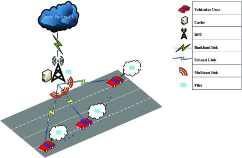
Figure 1: System model.

II System Model

We consider a vehicular downlink single-input single-output (SISO) transmission system, where a roadside unit (RSU), configured with one transmit antenna, provides hybrid multicast and unicast services to $K$ vehicular users (denoted by $U_{i}$, $i\in\{1,...,K\})$, equipped with a single antenna. As shown in Fig. 1, RSU is allocated with some cache resources, and the backhaul link of RSU is assumed to be capacity-limited. For simplicity of analysis, we study the case of a single one multicast group, i.e., $\left\{U_{i}\right\}$, while the case of multiple multicast groups will be extended in the future work.

II-A Transmission Model

Let ${x}_{M}$, ${x}_{i}=$ ($i\in\{1,...,K\}$) be the data symbols corresponding to multicast and unicast transmissions, respectively. All the data symbols are assumed to have the same unit power, i.e., $\text{E}[|x_{M}|^{2}]=\text{E}[|x_{i}|^{2}]=1$. It is assumed that RSU uses the NOMA protocol to send the superimposed signal to all users, which apply the SIC technique to decode the signal. To be realistic, we assume that the channel estimation processes are imperfect [References]. Hence, we have ${h}_{i}(t)=\sqrt{1-\phi^{2}}\hat{{{h}}}_{i}(t)+\phi{\epsilon}_{i}(t),$ where ${h}_{i}$ denotes the channel vector from RSU to $U_{i}$, $\hat{{{h}}}_{i}(t)\in\mathbb{C}^{Nt\times 1}$ denotes the estimated channel vector between the same nodes with variance $\Omega_{i}$, and ${\epsilon}_{i}\in\mathbb{C}^{Nt\times 1}$ denotes the estimation error vector with variance $\Omega_{\epsilon,i}$. For convenience, $\Omega_{\epsilon,i}$ is assumed to be a constant $\Omega_{\epsilon}$. All the channels are characterized by Jakes’ model [References] to measure users’ mobility, i.e., $\phi=J_{0}(2\pi f_{c}v_{i}/c\tau),$ where $J_{0}$ is the zeroth-order Bessel function of the first kind, $f_{c}$ denotes the carrier frequency, $v_{i}$ indicates the moving velocity of $U_{i}$, $c$ is the light speed, and $\tau$ represents the duration between two adjacent time slots. Without loss of generality, we sort the average power of ${\rm RSU}-U_{i}$ links as $|{h}_{1}|^{2}\geq\cdots\geq|{h}_{K}|^{2}$. For the sake of fairness, a minimum rate limitation, namely $r_{min}$ is set. The unicast rate of each user must satisfy $r_{i}^{U}\geq r_{min}$.

Considering any active time slot, RSU transmits a superimposed signal as ${z}=\sqrt{\beta_{M}P}{x}_{M}+\sum_{i=1}^{K}\sqrt{\beta_{U}P_{i}}{x}_{i},$ where $\beta_{M}$ and $\beta_{U}$ denote the power allocation coefficients for multicast and unicast transmissions, respectively; $P$ and $P_{i}$ $(\sum_{i=1}^{K}P_{i}=P)$ denote the transmit power in multicast layer and for $U_{i}$ in unicast layer, respectively. Let ${y}_{i}$ be the received signal at $U_{i}$, which is given as: ${y}_{i}=\sqrt{\beta_{M}P}{h}_{i}{x}_{M}+\sum_{j=1}^{K}\sqrt{\beta_{U}P_{j}}{h}_{i}{x}_{j}+n_{i},$ where $n_{i}\sim\mathcal{N}_{c}(0,\Omega_{0})$ is additive white Gaussian noise (AWGN). Because in the downlink system, multicast mode is more resource-efficient than unicast mode, multicast messages should have a higher priority [References]. Therefore, the multicast messages are assumed to be decoded and subtracted before decoding the unicast messages. Thus, the data rate of ${x}_{M}$ at $U_{i}$ can be obtained as

$$r_{i}^{M}=\log_{2}\left(1+\frac{\rho_{M}\lambda_{i}}{\rho_{U}\lambda_{i}+\Psi}\right),$$ (1)

where $\lambda_{i}=|\hat{{{h}}}_{i(n)}|^{2}$, $\rho_{M}=\beta_{M}P/\Omega_{0}$, $\rho_{U}=\beta_{U}P/\Omega_{0}$, $a=1/(1-\phi^{2})$, $b=\phi^{2}/(1-\phi^{2})\Omega_{\epsilon}$, and $\Psi=(\rho_{M}+\rho_{U})b+a$. Obviously, $\rho_{M}+\rho_{U}=\rho$, where $\rho=P/\Omega_{0}$. Similarly, the instantaneous rate of $x_{i}$ observed at $U_{i}$ can be derived as

$$r_{i}^{U}=\log_{2}\left(1+\rho_{i}\lambda_{i}/(\sum_{j=1}^{i-1}\rho_{j}\lambda_{i}+\sum_{j=1}^{i}\rho_{j}b+a)\right),$$ (2)

for $i\in\left\{1,...,K\right\}$, where $\rho_{i}=\beta_{U}P_{i}/\Omega_{0}$. The detailed derivations of (1) and (2) are shown in the end of this paper.

II-B Cache Model

We assume that the ergodic rate of the backhaul link between RSU and the core network is subject to $R$ bit/s/Hz. Besides, we assume that RSU is equipped with a finite capacity cache of size $N$. Let $\mathscr{F}=\{1,2,\cdots,F\}$ denote the content of $F$ files, each with normalized size of 1. Obviously, not all users can ask for their unicast messages at a time slot. As adopted in most existing works [References], the popularity profile on $\mathscr{F}$ is modeled by a Zipf distribution, with a skewness control parameter $\zeta$. Specifically, the popularity of file $f$ (denoted by $q_{f}$, $f\in\mathscr{F}$), is given by $q_{f}={f^{-\zeta}}/{\sum_{j=1}^{F}j^{-\zeta}},$ which follows $\sum_{f=1}^{F}q_{f}=1$. Let $c_{f}$ represent the probability that RSU caches the file $f$, satisfying $0\leq c_{f}\leq 1$. Due to cache capacity limit at RSU, we can obtain $\sum_{f=1}^{F}c_{f}\leq N$.

III Problem Formulation

Without loss of generality, the reception performance of multicast messages ${x}_{M}$ should meet the users’ quality of service (QoS) requirements, i.e., each user has a preset target rate $R_{M}$. As for unicast messages, they are assumed to be received opportunistically according to the user’s channel condition [References]. Therefore, we use the outage probabilities and instantaneous achievable rates to measure the reception performance of multicast and unicast messages, respectively.

III-A Outage Probability

Since the CDF of $\lambda_{i}$ is $F_{\lambda_{i}}(x)=1-\exp(-x/\Omega_{i})$, given the definition of the outage probability of ${x}_{M}$ at $U_{i}$ (denoted by $P_{i}^{M}$), namely, $P_{i}^{M}=\Pr\{r_{i}^{M}<R_{M}\}$, we have

$$P_{i}^{M} =1-\exp\left(-\frac{\Psi\theta_{M}}{(\rho_{M}-\theta_{M}\rho_{U})\Omega_{i}}\right),$$ (3)

where $\theta_{M}=2^{R_{M}}-1$. Obviously, $P_{i}^{M}>0$; in other words, we have $\rho_{U}<\rho/2^{R_{M}}$.

III-B Optimization Problem

Notably, our objective is to maximize the sum rate of unicast signals, and the optimization problem can be formulated as

$$P_{0}:\quad\mathop{\max\limits_{c_{f},\rho_{U},\rho_{i}}} \quad\sum_{i=1}^{K}r_{i}^{U}$$

$$s.t.\quad P_{i}^{M}<\delta,$$ (4a)

$$r_{i}^{U}\geq r_{min},$$ (4b)

$$\sum_{i=1}^{K}\rho_{i}=\rho_{U},$$ (4c)

$$\rho_{M}+\rho_{U}=\rho,$$ (4d)

$$\sum_{f=1}^{F}\sum_{i=1}^{K}q_{f}(1-c_{f})r_{i}^{U}\leq R,$$ (4e)

$$0\leq c_{f}\leq 1,$$ (4f)

$$\sum_{f=1}^{F}c_{f}\leq N,$$ (4g)

where (4a) and (4b) indicate the QoS requirements for the multicast and the unicast messages, respectively; (4c) and (4d) denote transmit power relationships for different signals; (4e) indicates the backhaul capacity constraint; (4f) indicates the value range of cache probability; (4g) represents the cache capacity limit at the RSU. Without loss of generality, we have the outage requirement $\delta$ satisfying $0<\delta<1$, i.e., $\ln(1-\delta)<0$. Therefore, by substituting (3) and (4d) into (4a), for $\rho_{U}<\rho/2^{R_{M}}$, we can arrive at $\rho_{U}\leq{\Psi\theta_{M}}/{(2^{R_{M}}\Omega_{i}\ln(1-\delta))}+{\rho}/{2^{R_{M}}}.$ Therefore, $P_{0}$ can be equivalently rewritten as

$$P_{1}:\quad\mathop{\max\limits_{c_{f},\rho_{U},\rho_{i}}} \quad\sum_{i=1}^{K}r_{i}^{U}$$

$$s.t.\quad \rho_{U}\leq\frac{\Psi\theta_{M}}{2^{R_{M}}\Omega_{1}\ln(1-\delta)}+\frac{\rho}{2^{R_{M}}},$$ (5a)

$$(\ref{4b}),(\ref{4c}),(\ref{4e})-(\ref{4g}).$$

IV Proposed Lower Bound Relaxation Method

Evidently, the objective function of $P_{1}$ is non-convex and hard to solve. Moreover, as shown in (2), $(\lambda_{i}+b)$ in the denominator makes $r_{i}^{U}$ hardly be reformulated. Therefore, we use the lower bound relaxation method, which can be derived as

$$r_{i}^{U}=\log_{2}\left(1+\rho_{i}\lambda_{i}/(\sum_{j=1}^{i-1}\rho_{j}\lambda_{i}+\Psi)\right).$$ (6)

The detailed derivation of (6) is shown in the end of this paper. Invoking [References], $\rho_{U}$ can be split into two parts: $\rho_{min}$ for $r_{min}$ and $\triangle\rho$ for $\sum_{i=1}^{K}\triangle r_{i}^{U}$. The minimum transmit signal-to-noise ratio (SNR) and the excess transmit SNR of $U_{i}$ are denoted by $\rho_{i,min}$ and $\triangle\rho_{i}$, respectively. Apparently, we have $\rho_{min}=\sum_{i=1}^{K}\rho_{i,min}$ and $\triangle\rho=\sum_{i=1}^{K}\triangle\rho_{i}$. For convenience, we use $\rho_{sum}^{min}$ to represent the sum of $\rho_{i,min}$, i.e., $\rho_{sum}^{min}=\sum_{i=1}^{K}\rho_{i,min}$. After several mathematical steps, we can obtain Propositions 1 and 2. See Appendix A for the proofs of them.

Proposition 1: With fixed $r_{min}$, we have

$$\rho_{sum}^{min}=(2^{r_{min}}-1)\sum_{i=0}^{K-1}{2^{ir_{min}}}/{\lambda_{K-i}},$$ (7)

and

$$\sum_{i=1}^{K}r_{i}^{U}=Kr_{min}+\sum_{i=1}^{K}\triangle r_{i}^{U}.$$ (8)

For ease of representation, by defining

$$\rho_{i}^{e}=(\triangle\rho_{i}-(2^{r_{min}}-1)\sum_{j=1}^{i-1}\triangle\rho_{j})2^{(K-i)r_{min}},$$ (9)

and $n_{i}^{e}=(\Psi/\lambda_{i}+\sum_{j=1}^{i}\rho_{j,min})2^{(K-i)r_{min}},$ we can arrive at $\triangle r_{i}^{U}=\log_{2}\left(1+{\rho_{i}^{e}}/{(n_{i}^{e}+\sum_{j=1}^{i-1}\rho_{j}^{e})}\right).$

Proposition 2: The more power we allocate to the users with stronger channel conditions, the higher the sum rate is. In other words, when all the excess power is allocated to $U_{1}$, we have the optimal solution as $\sum_{i=1}^{K}\triangle r_{i}^{U}=\triangle r_{1}^{U}=\log_{2}(1+{(\rho_{U}-\rho_{sum}^{min})\lambda_{1}}/{(\Psi 2^{Kr_{min}})})$.

Occupying the Propositions above, $P_{1}$ can be derived as

$$P_{2}:\quad\mathop{\max\limits_{c_{f},\rho_{U},\rho_{i}}} \quad Kr_{min}+\sum_{i=1}^{K}\triangle r_{i}^{U}$$

$$s.t.\quad (\ref{4c}),(\ref{4f}),(\ref{4g}),(\ref{5a}),$$

$$Kr_{min}\!\!+\!\!\sum_{i=1}^{K}\triangle r_{i}^{U}\leq\frac{R}{\sum_{f=1}^{F}q_{f}(1-c_{f})},$$ (10a)

$$\triangle r_{i}^{U}=\log_{2}\left(1+\frac{\rho_{i}^{e}}{n_{i}^{e}+\sum_{j=1}^{i-1}\rho_{j}^{e}}\right).$$ (10b)

Obviously, $P_{2}$ is still hard to solve due to (4c), (5a), and (10a). If we can fix $\rho_{i}$, $P_{2}$ will be facilitated. Therefore, our aim is to find a value of $\rho_{U}$ which always satisfies (4c) and (5a), with any distribution of $\rho_{i}$. To elaborate a little further, first, we assume to allocate all excess power to $U_{1}$ as shown in Proposition 2. Obviously, this is the maximum value of the objective function which $\rho_{i}$ can achieve in various distributions and also the strictest (10a) limitation. In this case, (10a) can be rewritten as $Kr_{min}+\triangle r_{1}^{U}\leq{R}/{(\sum_{f=1}^{F}q_{f}(1-c_{f}))}$. Apparently, $\rho_{U}=0$ is a feasible point, which leads to $\rho_{min}=0$, $\triangle\rho=0$, and $r_{min}=0$. In this case, (5a) and (10a) are bound to be satisfied. Consequently, we can achieve $P_{3}$ as

$$P_{3}:\quad\mathop{\max\limits_{c_{f},\rho_{U}}} \quad\text{obj}=Kr_{min}+\triangle r_{1}^{U}$$

$$s.t.\quad (\ref{4f}),(\ref{4g}),(\ref{5a}),(\ref{8a}),$$

$$\triangle r_{1}^{U}=\log_{2}\left(1+\frac{(\rho_{U}-\rho_{sum}^{min})\lambda_{1}}{\Psi 2^{Kr_{min}}}\right),$$ (11a)

$$\rho_{sum}^{min}=(2^{r_{min}}-1)\sum_{i=0}^{K-1}\frac{2^{ir_{min}}}{\lambda_{K-i}}.$$ (11b)

However, $P_{3}$ is still non-convex. Hence, we divide it into two convex sub-problems to find its optimal solution. For given $c_{f}$, problem $P_{3}$ reduces to

$$P_{4}:\quad\mathop{\max\limits_{\rho_{U}}}$$ obj

$$s.t.\quad (\ref{5a}),(\ref{8a}),(\ref{9e}),(\ref{9f}).$$

For given $\rho_{U}$, problem $P_{3}$ reduces to

$$P_{5}:\quad\mathop{\max\limits_{c_{f}}}$$ obj

$$s.t.\quad (\ref{4f}),(\ref{5a}),(\ref{8a}),(\ref{9f}).$$

Based on $P_{4}$ and $P_{5}$, we can obtain the lower bound of the optimal solution of $P_{3}$ in Algorithm 1.

Algorithm 1 Algorithm for Solving The Problem

1:System Parameters, $Converge$=false, iteration index $l=1$, and tolerance $\delta$.

2:System sum rate.

3:while $Converge$=false do

4:     $l=l+1$;

5:     Solve $P_{4}$ for current $\rho_{U}^{(l)}$.

6:     With $\rho_{U}^{(l)}$, solve $P_{5}$ for current $c_{f}^{(l)}$.

7:     Calculate $\text{obj}^{(l)}$.

8:     if $|\text{obj}^{(l)}-\text{obj}^{(l-1)}|\leq\delta$ then

9:         $Converge$=ture, $\text{obj}^{*}=\text{obj}^{(l)}$.

10:     end if

11:end while

12:return Optimal system sum rate $\text{obj}^{*}$.

Lemma 1.

Algorithm 1 guarantees convergence.

Proof.

Cauchy’s theorem proves that function with compact and continuous constraint set always converges. Besides, solving $P_{4}$ and $P_{5}$ alternatively guarantees the convergence [References]. Therefore, proposed algorithm is convergent. ∎

Lemma 2.

The time complexity of Algorithm 1 is $\mathcal{O}(\frac{1}{\delta^{2}})$.

Proof.

The complexity of sub-linear rate, e.g., $f^{(l)}-f^{*}\leq\delta$ is $\mathcal{O}(\frac{1}{\delta^{2}})$. Therefore, the complexity of the proposed algorithm is obtained. ∎

V Numerical Results

In this section, we discuss the performance of the proposed cache-aided NOMA, and compare it with the cache-aided OMA systems. The transmit power at RSU is set as $P=10$w and the backhaul capacity constraint is set as $R=5$ bit/s. We consider that RSU serves $K=2$ and $K=3$ vehicles respectively. For convenience, we set $(\Omega_{1},\Omega_{2})=(10,5)$ for the scenario where $K=2$, and $(\Omega_{1},\Omega_{2},\Omega_{3})=(10,5,1)$ for the scenario where $K=3$. In addition, the detailed settings of the Jakes’ model are shown as follows: $v_{i}$ = 150 km/h, which is practical especially for a highway scenario; $f_{c}=5.9$GHz; $\tau=10^{-6}$. The noise power is set as $\Omega_{0}=1$w. As for the CSI estimation errors, we set $\Omega_{\epsilon}=0.1$. The outage probability threshold for multicast service is set as $\delta=0.1$.

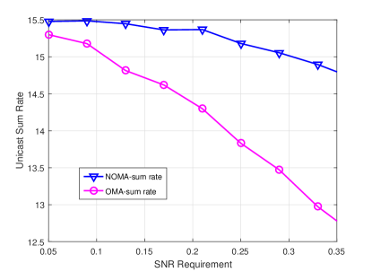
(a) $K$=2

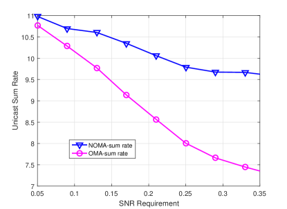
(b) $K$=3

Figure 2: Sum-rate versus minimum rate constraint with cache size $N=2$.

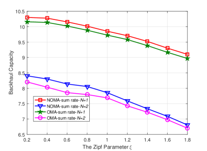
(a) $K$=2

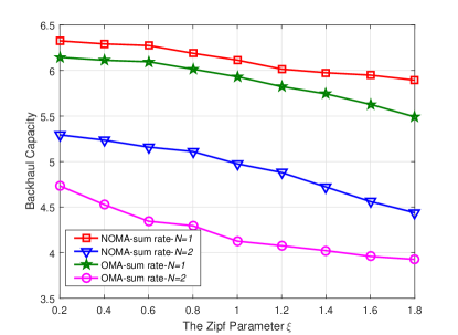
(b) $K$=3

Figure 3: Backhaul capacity versus cache size with minimum rate constraint $r_{min}=0.2$.

In Fig. 2, we compare the unicast sum rate of cache-aided NOMA with that of the OMA counterpart under different minimum rate constraints. As expected, the NOMA scheme outperforms the OMA one in all cases. Obviously, the sum rates decrease when $r_{min}$ increases, but the decrease is moderate. This is because $Kr_{min}$ is linearly increased while $\triangle r_{1}^{U}$ is exponentially decreased. Furthermore, compare Figs. 2(a) and 2(b), we can easily find that the systems with three users have lower unicast sum rate. This is because when the transmission power of the RSU is fixed, the increase of the user will also aggravate the interference, which leads to the decrease of the receiving performance, and finally affects the unicast rate.

Figure 3 shows the backhaul capacity versus the zipf parameter $\xi$ for different cache size $N$. Obviously, as $\xi$ increases, the backhaul capacity decreases, which comes from the fact that larger $\xi$ represents the more concentrated request hotspots. In other words, the probabilities that the cached files at RSU are requested by users are larger, which reduces the backhaul overhead. Moreover, one can observe that the backhaul capacity of the NOMA scheme is always larger than that of the OMA one. This is because, compared to OMA, NOMA shows a superior unicast rate performance and therefore requires a relatively higher amount of backhaul resources. Besides, we can find that an increasing number of users will decrease the backhaul capacity, whose cause is the same as that of the previous figure.

VI Conclusions

In this paper, we have incorporated multicast and unicast services into a cache-aided SISO vehicular NOMA system with high mobility. We have formulated an optimization problem to maximize the unicast sum rate subject to the peak power, the backhaul capacity, the minimum unicast rate, and the maximum multicast outage probability constraints. The proposed non-convex problem has been appropriately solved by the proposed lower bound relaxation method. Simulation results have demonstrated that our proposed cache-aided NOMA scheme outperforms the OMA counterpart.

Appendix A Proofs of Propositions 1 and 2

Being allocated $\rho_{i,min}$, the unicast rate of $U_{i}$ can achieve $r_{min}$, i.e.,

$$r_{min}=\log_{2}\left(1+\rho_{i,min}\lambda_{i}/(\sum_{j=1}^{i-1}\rho_{j,min}\lambda_{i}+\Psi)\right),$$ (A.1)

which yields

$$2^{r_{min}}-1=\rho_{i,min}/(\sum_{j=1}^{i-1}\rho_{j,min}+\Psi/\lambda_{i}).$$ (A.2)

Using partition ratio theorem, (A.2) can be formulated as

$$\frac{(2^{r_{min}}-1)\sum_{j=1}^{i-1}\triangle\rho_{j}}{\sum_{j=1}^{i-1}\triangle\rho_{j}}=\frac{\rho_{i,min}}{\sum_{j=1}^{i-1}\rho_{j,min}+\Psi/\lambda_{i}}$$

$$=\frac{\rho_{i,min}+(2^{r_{min}}-1)\sum_{j=1}^{i-1}\triangle\rho_{j}}{\sum_{j=1}^{i-1}\rho_{j,min}+\sum_{j=1}^{i-1}\triangle\rho_{j}+\Psi/\lambda_{i}}.$$ (A.3)

Substituting (A) into (A.1), we can obtain

$$r_{min}=\log_{2}\left(1+\frac{\rho_{i,min}+(2^{r_{min}}-1)\sum_{j=1}^{i-1}\triangle\rho_{j}}{\sum_{j=1}^{i-1}\rho_{j}+\Psi/\lambda_{i}}\right).$$ (A.4)

Therefore, $\triangle r_{i}^{U}$ can be expressed as

$$\triangle r_{i}^{U} =r_{i}^{U}-r_{min}$$

$$= \log_{2}\left(1+\frac{\triangle\rho_{i}-(2^{r_{min}}-1)\sum_{j=1}^{i-1}\triangle\rho_{j}}{\sum_{j=1}^{i}\rho_{j,min}+\frac{\Psi}{\lambda_{i}}+2^{r_{min}}\sum_{j=1}^{i-1}\triangle\rho_{j}}\right)$$

$$= \log_{2}(1+\frac{\mathscr{P}_{i}}{\mathscr{N}_{i}+\mathscr{Q}_{i}}),$$ (A.5)

where $\mathscr{P}_{i}=\triangle\rho_{i}-(2^{r_{min}}-1)\sum_{j=1}^{i-1}\triangle\rho_{j}$, $\mathscr{N}_{i}=\sum_{j=1}^{i}\rho_{j,min}+\frac{\Psi}{\lambda_{i}}$, and $\mathscr{Q}_{i}=2^{r_{min}}\sum_{j=1}^{i-1}\triangle\rho_{j}$. Using the properties of recurrence, we have

$$\mathscr{Q}_{i}=2^{r_{min}}\sum_{j=1}^{i-1}\triangle\rho_{j}=\sum_{j=1}^{i-1}(2^{r_{min}})^{i-j}\mathscr{P}_{j}.$$ (A.6)

Let $\rho_{i}^{e}$ denote $\mathscr{P}_{i}(2^{r_{min}})^{K-i}$. Then, we can rewrite (A.6) into $\mathscr{Q}_{i}(2^{r_{min}})^{K-i}=\sum_{j=1}^{i-1}(2^{r_{min}})^{K-j}\mathscr{P}_{j}=\sum_{j=1}^{i-1}\rho_{j}^{e}.$ Therefore, we can derive

$$\triangle r_{i}^{U}=\log_{2}(1+\frac{\rho_{i}^{e}}{n_{i}^{e}+\sum_{j=1}^{i-1}\rho_{j}^{e}}),$$ (A.7)

where $n_{i}^{e}=(\Psi/\lambda_{i}+\sum_{j=1}^{i}\rho_{j,min})2^{(K-i)r_{min}}.$ On the other hand, (A.2) can be rewritten as $\rho_{i,min}=(2^{r_{min}}-1)(\sum_{j=1}^{i-1}\rho_{j,min}+\Psi/\lambda_{i}).$ After the recurrence operation, we have

$$\rho_{i,min}=\frac{2^{r_{min}}-1}{\lambda_{i}}+\frac{(2^{r_{min}}-1)^{2}2^{(i-j-1)r_{min}}}{\lambda_{i}},$$ (A.8)

which results in $\rho_{sum}^{min}=\sum_{i=1}^{K}\rho_{i,min}=(2^{r_{min}}-1)\sum_{i=0}^{K-1}{2^{ir_{min}}}/{\lambda_{K-i}}.$ Because $\rho_{sum}^{min}$ represents all the excess power, $\rho_{i}^{e}\leq\rho_{sum}^{min}$. Therefore, when $i=1$, $\rho_{i}^{e}=\rho_{sum}^{min}$, (A.7) achieves its optimal value. The proofs complete.

Appendix B Supplementary Material

B-A The Detailed Derivations of (1) and (2)

As we know, the transmit signal at RSU is

$${z}=\sqrt{\beta_{M}P}{x}_{M}+\sum_{i=1}^{K}\sqrt{\beta_{U}P_{i}}{x}_{i},$$ (B.1)

where $\text{E}[|x_{M}|^{2}]=\text{E}[|x_{i}|^{2}]=1$. Then the received signal at user $i$ can be derived as

$${y}_{i}=\sqrt{\beta_{M}P}{h}_{i}{x}_{M}+\sum_{j=1}^{K}\sqrt{\beta_{U}P_{j}}{h}_{i}{x}_{j}+n_{i},$$ (B.2)

which can be rewritten as

$${y}_{i} =\sqrt{\beta_{M}P}\sqrt{1-\phi^{2}}\hat{{{h}}}_{i}{x}_{M}$$

$$\overbrace{+\sqrt{\beta_{M}P}\phi{\epsilon}_{i}{x}_{M}+\sum_{j=1}^{K}\sqrt{\beta_{U}P_{j}}(\sqrt{1-\phi^{2}}\hat{{{h}}}_{i}a+\phi{\epsilon}_{i}){x}_{j}+n_{i}}^{interference}.$$ (B.3)

Without loss of generality, multicast message always has a higher priority than the unicast one. Therefore, the receiver should first decode the multicast message ($x_{M}$) and subtract it from $y_{i}$. In this way, the SINR of $x_{M}$ at user $i$ can be obtained by

$$\gamma_{i}^{M} ={\beta_{M}P(1-\phi^{2})|\hat{{{h}}}_{i}|^{2}}$$

$$\div\left(\beta_{M}P\phi^{2}|{\epsilon}_{i}|^{2}+\sum_{j=1}^{K}\beta_{U}P_{j}(1-\phi^{2})|\hat{{{h}}}_{i}|^{2}\right.$$

$$\left.+\sum_{j=1}^{K}\beta_{U}P_{j}\phi^{2}|{\epsilon}_{i}|^{2}+\Omega_{0}\right),$$ (B.4)

which equals to the SINR in (1). After decoding $x_{M}$, user $i$ aims to obtain $x_{i}$ from the superposed signal

$${y}_{i}=\sum_{j=1}^{K}\sqrt{\beta_{U}P_{j}}{h}_{i}{x}_{j}+n_{i}.$$ (B.5)

Recall $|h_{1}|^{2}\geq\cdots\geq|h_{i}|^{2}\geq\cdots\geq|h_{K}|^{2}$, user i first decodes the data symbols for the users with weaker channels, subtract them through SIC technique, and then decoding the data symbol for itself. Consequently, we can obtain

$${y}_{i} =\sqrt{\beta_{U}P_{i}}\sqrt{1-\phi^{2}}\hat{{{h}}}_{i}{x}_{i}$$

$$+\overbrace{\sum_{j=1}^{i-1}\sqrt{\beta_{U}P_{j}}(\sqrt{1-\phi^{2}}\hat{{{h}}}_{i}+\phi{\epsilon}_{i}){x}_{j}+\sqrt{\beta_{U}P_{i}}\phi{\epsilon}_{i}{x}_{i}+n_{i}}^{interference},$$ (B.6)

and

$$\gamma_{i}^{U}=\frac{{\beta_{U}P_{i}}{(1-\phi^{2})}|\hat{{{h}}}_{i}|^{2}}{\sum_{j=1}^{i-1}{\beta_{U}P_{j}}{(1-\phi^{2})}|\hat{{{h}}}_{i}|^{2}+\sum_{j=1}^{i}{\beta_{U}P_{j}}\phi^{2}|{\epsilon}_{i}|^{2}+\Omega_{0}}.$$ (B.7)

In this way, we can finally derive (1) and (2).

B-B The Derivation of (6)

Recall the instantaneous rate of $x_{i}$ observed at $U_{i}$, i.e.,

$$r_{i}^{U}=\log_{2}\left(1+\rho_{i}\lambda_{i}/(\sum_{j=1}^{i-1}\rho_{j}\lambda_{i}+\overbrace{\sum_{j=1}^{i}\rho_{j}b+a}^{relax})\right).$$ (B.8)

Since the last two parts in the denominator are hardly handled, we herein use the lower bound relaxation method and replace them by a constant, i.e.,

$$\sum_{j=1}^{i}\rho_{j}b+a=\sum_{j=1}^{i}\frac{\beta_{U}P_{i}}{\Omega_{0}}b+a\underset{i\rightarrow K}{\overset{\beta_{U}\rightarrow 1}{\rightarrow}}\sum_{j=1}^{K}\rho b+a=\Psi.$$ (B.9)

In this way, we can derive (6).

References

• [1] M. Fallgren et al., “Multicast and broadcast enablers for high-performing cellular V2X systems,” IEEE Trans. Broadcast., vol. 65, no. 2, pp. 454–463, Jun. 2019.
• [2] E. Chen, M. Tao, and Y. Liu, “Joint base station clustering and beamforming for non-orthogonal multicast and unicast transmission with backhaul constraints,” IEEE Trans. Wireless Commun., vol. 17, no. 9, pp. 6265–6279, Sept. 2018.
• [3] D. Lecompte and F. Gabin, “Evolved multimedia broadcast/multicast service (eMBMS) in LTE-advanced: overview and Rel-11 enhancements,” IEEE Commun. Mag., vol. 50, no. 11, pp. 68–74, Nov. 2012.
• [4] D. Wan, M. Wen, F. Ji, H. Yu, and F. Chen, “Non-orthogonal multiple access for cooperative communications: Challenges, opportunities, and trends,” IEEE Wireless Commun., vol. 25, no. 2, pp. 109–117, Apr. 2018.
• [5] Z. Ding, Z. Yang, P. Fan, and H. V. Poor, “On the performance of non-orthogonal multiple access in 5G systems with randomly deployed users,” IEEE Signal Process. Lett., vol. 21, no. 12, pp. 1501–1505, Dec. 2014.
• [6] L. Dai, B. Wang, Y. Yuan, S. Han, C-L. I, and Z. Wang, “Non-orthogonal multiple access for 5G: solutions, challenges, opportunities, and future research trends,” IEEE Commun. Mag., vol. 53, no. 9, pp. 74–81, Sept. 2015.
• [7] S. K. Datta, J. Haerri, C. Bonnet, and R. Ferreira Da Costa, “Vehicles as connected resources: opportunities and challenges for the future,” IEEE Veh. Technol. Mag., vol. 12, no. 2, pp. 26–35, Jun. 2017.
• [8] Z. Ding, P. Fan, G. K. Karagiannidis, R. Schober, and H. V. Poor, “NOMA assisted wireless caching: strategies and performance analysis,” IEEE Trans. Commun., vol. 66, no. 10, pp. 4854-4876, Oct. 2018.
• [9] M. Tao, E. Chen, H. Zhou, and W. Yu, “Content-centric sparse multicast beamforming for cache-enabled cloud RAN,” IEEE Trans. Wireless Commun., vol. 15, no. 9, pp. 6118–6131, Sept. 2016.
• [10] Y. Chen, L.Wang, Y. Ai, B. Jiao, and L. Hanzo, “Performance analysis of NOMA-SM in vehicle-to-vehicle massive MIMO channels,” IEEE J. Sel. Areas Commun., vol. 35, no. 12, pp. 2653–2666, Dec. 2017.
• [11] B. Di, L. Song, Y. Li, and Z. Han, “V2X meets NOMA: non-orthogonal multiple access for 5G-enabled vehicular networks,” IEEE Wireless Commun., vol. 24, no. 6, pp. 14–21, Dec. 2017.
• [12] S. Gurugopinath, P. C. Sofotasios, Y. Al-Hammadi, and S. Muhaidat, “Cache-aided non-orthogonal multiple access for 5G-enabled vehicular networks,” IEEE Trans. Veh. Technol., vol. 68, no. 9, pp. 8359–8371, Sept. 2019.
• [13] K. S. Ahn and R. W. Heath, “Performance analysis of maximum ratio combining with imperfect channel estimation in the presence of cochannel interferences,” IEEE Trans. Wireless Commun., vol. 8, no. 3, pp. 1080–1085, Mar. 2009.
• [14] Y. M. Khattabi and M. M. Matalgah, “Alamouti-OSTBC wireless cooperative networks with mobile nodes and imperfect CSI estimation,” IEEE Trans. Veh. Technol., vol. 67, no. 4, pp. 3447–3456, Apr. 2018.
• [15] G. Araniti, C. Campolo, M. Condoluci, A. Iera, and A. Molinaro, “LTE for vehicular networking: a survey,” IEEE Commun. Mag., vol. 51, no. 5, pp. 148-157, May 2013.
• [16] S. H. Chae and W. Choi, “Caching placement in stochastic wireless caching helper networks: Channel selection diversity via caching,” IEEE Trans. Wireless Commun., vol. 15, no. 10, pp. 6626–6637, Oct. 2016.
• [17] Z. Chen, Z. Ding, X. Dai, and R. Zhang, “An optimization perspective of the superiority of NOMA compared to conventional OMA,” IEEE Trans. Signal Process., vol. 65, no. 19, pp. 5191–5202, Oct. 2017.
• [18] S. Boyd and L.Vandenberghe, Convex Optimization, New York, NY, USA: Cambridge Univ. Press, 2004.