GLISSE: A GPU-optimized planetary system integrator with application to orbital stability calculations.

Abstract

We present a GPU-accelerated numerical integrator specifically optimized for stability calculations of small bodies in planetary systems. Specifically, the integrator is designed for cases when large numbers of test particles (tens or hundreds of thousands) need to be followed for long durations (millions of orbits) to assess the orbital stability of their initially “close-encounter free” orbits. The GLISSE (Gpu Long-term Integrator for Solar System Evolution) code implements several optimizations to achieve a roughly factor of 100 speed increase over running the same code on a CPU. We explain how various hardware speed bottlenecks can be avoided by the careful code design, although some of the choices restrict the usage to specific types of application.

As a first application, we study the long-term stability of small bodies initially on orbits between Uranus and Neptune. We map out in detail the small portion of the phase space in which small bodies can survive for 4.5 billion years of evolution; the ability to integrate large numbers of particles allow us to identify for the first time how instability-inducing mean-motion resonance overlaps sharply define the stable regions. As a second application, we map the boundaries of 4 Gyr stability for transneptunian objects in the 5:2 and 3:1 mean-motion resonances, demonstrating that long-term perturbations remove the initially stable Neptune-crossing members.

1 Introduction

A common class of problems in planetary system dynamics is to study the motion of a large number $N$ of low-mass bodies (asteroids, comets, dust grains) moving in the gravitational field of a central massive object (a star or a planet) and a small number ($N_{p}$) massive objects (planets around a star, or moons around a planet). While the central object and massive objects need to be evolved using the usual $N_{p}^{2}$ approach, the low-mass objects can be treated as test particles (denoted as just ‘particles’ hereafter) and thus the total calculation expense scales as $N_{p}^{2}+NN_{p}\approx NN_{p}$ once the number of particles is large enough. Because the particles are approximated as not having enough individual (or total) mass to affect other particles, numerically computing their time evolution requires only a knowledge of the planetary positions. In numerical planetary dynamics, the problem is usually implemented in algorithm that integrates the planets forward one time step, advances the particles one step, and then repeats. This style of algorithm has often been implemented on both single processors and on clusters, where parallelization to study large numbers of test particles is accomplished by repeating the (relatively low-cost) integration of the planetary evolution on every compute core of the cluster, each of which has its own set of unique test particles. Dedicated N-body hardware [like GRAPE; see reference 1, for example] allows faster acceleration evaluation but are not easily available and do not inherently deploy massive test-particle parallelism.

Graphics Processing Units (GPUs) are special purpose hardware cards whose primary purpose is to rapidly render images for display purposes; in particular, they are optimized to manipulate large blocks of data in a highly parallel fashion. This makes them incredibly powerful, for example, in ray tracing or computer gaming. GPU-accelerated computing has brought much utility to applications such as deep learning and computer graphics [2, 3]. There was much initial excitement about GPUs in many domains of scientific computing, but in many cases the speed improvements that are attained via GPUs are modest especially when compared to the cost of adding GPU units into a computer system. The issue has typically been that the scientific problem requires one or more of (A) double precision, which is slower to run and often by a factor of more than two, (B) a large amount of data transfer, and/or (C) a need to treat different particles differently. An example of the latter in planetary dynamics would be a need to use variable integration time steps to deal with close encounters. As a result [4], planetary dynamics has rarely had the same kind of speed improvements due to the need to formulate problems in a form that GPUs can efficiently solve, despite GPU libraries for N-body planetary mutual interaction being available [5, 6, 7] or stellar dynamics [e.g., 8, 9].

Despite this, the large-scale simulation of massless test particles is at first glance highly suitable for GPU simulation as there is no interaction between individual particles. In this paper, we present a GPU software package that facilitates the integration of large populations of test particles that avoid close encounters in planetary systems.

We provide two examples of problems that can be sped up by using our software. In the first, we provide a study of stable (surviving for the $\sim$4.5 Gyr age of the Solar system) phase space between Uranus and Neptune. In the second, we investigate objects in the 3:1 and 5:2 resonances with Neptune and in particular the boundaries of the librating portions of the resonance in ($a,e$) space on both short (Myr) and 4 Gyr time scales.

2 Structure of the Software

We have developed the GLISSE integrator as a software package written in CUDA C++. In this section, we explain the code’s design and study the relative peformance of the CPU+GPU combination compared to CPU only codes and another GPU integrator.

2.1 Hardware constraints

GPU algorithms should be designed with hardware considerations in mind. As the popularity of using GPUs to accelerate calculations has grown, GPUs have also become more versatile. Newer generations of GPUs contain tensor cores to accelerate matrix multiplication or raytracing cores to accelerate the computation of intersections between geometry primitives. However, there has been no mainstream development of GPU hardware that is specialized for the simulation of orbital dynamics. Problems in orbital dynamics thus need to be approached using general GPU compute cores. Large performance gains can still be made by optimally making use of the parallel capabilities of GPUs, by using a detailed understanding of the architecture and its potential pitfalls.

For general computing, the motivation to use a GPU is in the large number of arithmetic units (CUDA cores in the NVIDIA GPU language) available for parallel processing. While consumer grade CPUs typically have on the order of 4-8 cores, GPU core count can range from hundreds to thousands in a single chip. The base clock speed of GPU cores is slower than the average CPU, which is more than made up for by the sheer number of cores available. GPUs are therefore outperformed by CPUs in cases where number of needed parallel calculations is small. As a first guideline, the scale of problems needs to be large before seeing significant speedups. This is an excellent match for orbital dynamics simulations where the number of particles that need to be simulated is large (hundreds of thousands and even millions).

Differences in architecture between CPUs and GPUs make it necessary to approach implementation differently. The NVIDIA CUDA drivers provide interfaces to control a GPU through C or C++ Application Programming Interfaces (APIs). GPUs are used to replace performance-critical sections of CPU code by offloading functions to the GPU. These functions that run on the GPU are named ‘kernels’ and can be written similarly to CPU code. Kernels cannot access CPU memory directly, but instead access GPU memory that often contains data transferred from the CPU over a data bus (Figure 1). The kernel is launched from the CPU, where function arguments, thread count, and ‘block’ size can be specified. A thread is a unit of work that the GPU performs; each thread runs the function specified in the kernel once. Threads are further divided into groups named ‘blocks’. Blocks are are physically executed by ‘streaming multiprocessors’ (SMs) on the GPU chip, 13 of which are present on the Tesla K20m which we primarily used. Each SM can run up to two blocks concurrently, but we run one block per SM due to memory constraints. The kernel launch is completed when all the launched threads are finished (i.e. when all blocks are executed by a SM). When there are more blocks to process than the SMs on the device can run concurrently, the GPU ‘thread scheduler’ maintains a queue of yet unprocessed blocks and distributes the blocks as SMs become free from previous work. A block can only finish when all threads in that block are completed. Thus, any situation in which a single thread requires more computational work than another in the same block results in the entire block waiting for more expensive threads to finish. An explicit example would be if one had an iterative component in an algorithm, and difficult cases would require more iterations to converge to a desired precision. The entire block then takes as long as the ‘worst case’ thread. It is therefore beneficial to compute problems on the GPU where work can be evenly distributed across threads.

GPU computation is also subject to a phenomenon called ‘branch divergence’, which is a more serious bottleneck here than in CPUs. In the design of GLISSE, branch divergence places constraints on the ways in which we implement the iterative Kepler equation solver. Due to the parallel nature of SMs, threads within the same block must concurrently execute the same code at all times. When execution paths on a block diverge (e.g. due to ‘if’ or ‘while’ statements), the different paths are computed sequentially, instead of concurrently. In practice, a loop that runs a different number of times on different threads will take as long as the slowest thread takes to complete.

This is important since testing for convergence in an iterative equation solver can often result in varying loop lengths for different input values. One consequence of this is that particles which take exceptionally long to converge will result in major performance losses, so it may be beneficial to simply disable such particles to keep the simulation running at maximum speed. However, there can also be performance losses from situations where particles within the same block perform largely different types of calculations depending on the state of the particle.

Finally, data transfers may also present a performance bottleneck. A GPU cannot perform computation directly on CPU memory, so data must be first copied to the GPU, which can incur performance costs. However, to mitigate this issue, data can be transferred to the GPU while a kernel is active. By preparing data for the next kernel launch while a kernel is already running on the GPU, the time cost of data transfers can be partially or completely avoided. Further, reads and writes on the GPU are cached. Instead of reading and writing directly to GPU memory, data must pass through the cache first (Figure 1), which is efficient for applications where data is stored and accessed sequentially. GLISSE is cache efficient by its use of a kernel that minimizes non-sequential data access in global memory: for each particle, data is read once at the beginning of a planetary chunk, and written once at the end of a planetary chunk.

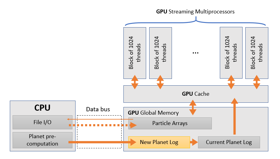
Figure 1: Schematic representation of the how the GLISSE algorithm interacts with the CPU and GPU hardware. The planetary position history/log for a ’planet chunk’ of time is pre-computed on the CPU while the GPU advances the test particles over the previous planet log; once completed, the CPU pushes the new planet log to the GPU (usually before the GPU finishes the test particle propagation over the last planet chunk). Note that the test particle arrays are pushed to the GPU only at code start, and are only returned to the CPU infrequently (for trajectory logging and at code end).

2.2 Implementation

To achieve superior performance with GLISSE, we have adapted the implementation to the specific problems that GLISSE is designed to solve (orbital stability calculations in a planetary context). We benefit from the fact that systems GLISSE is designed for have a large number of non-interacting (negligible-mass) particles, and thus the GPU is exclusively used to perform large-scale integration of these test particles.

For planets, GLISSE computes the planetary evolution on the CPU in near-parallel with the GPU. Part of the reason for the high performance of GLISSE is because a small future portion the planetary history is pre-computed in ‘chunks’ because all the test particles will need to share the planetary positions. However, the fully interacting planetary evolution computation does not benefit from the GPU architecture. We thus compute the planetary positions forward in time for a number of time steps (called the user-configurable ‘planetary chunk size’, say 128 or 1024) on the CPU first, with a standard Wisdom-Holman mixed-variable symplectic algorithm, MVS [10]. GLISSE’s CPU planetary integration using MVS requires that there are no close encounters between massive bodies; in principle, an algorithm that handles planetary encounters could be substituted. This time evolution is stored into a ‘planet log’ for the coming GPU steps for that planetary chunk’s period; because only the planetary positions matter for the test-particle evolution, only those position arrays need be loaded over to the GPU. At code start, a first planet chunk is computed and that log passed to the GPU; once the GPU is advancing test particles for that planet chunk, the CPU pre-computes the next planet chunk and preloads it to the GPU before the test particles are completely advanced. In this way there is essentially zero overhead in computing the planetary evolution ‘on the fly’ as the test-particle calculation is performed.

For the test particle integration, we use a slightly-altered version of the MVS algorithm, which approximates the Hamiltonian for a single particle by

$$H=H_{Kepler}+H_{int},$$ (1)

which is analytically split into two exactly-solvable Hamiltonians (expressed per unit mass $m_{1}$ for the test particles):

$$\begin{split}\frac{H_{Kepler}}{m_{1}}&=\frac{v_{1}^{\prime 2}}{2}-\frac{Gm_{0}}{\|r^{\prime}_{1}\|}\\ \frac{H_{int}}{m_{1}}&=-\sum_{j=2}^{N_{p}+1}\left(\frac{Gm_{j}}{\|\bf{r}_{j1}\|}-\frac{Gm_{j}\bf{r^{\prime}}_{1}\cdot\bf{r}_{j0}}{\|\bf{r}_{j0}\|^{3}}\right),\end{split}$$ (2)

where primed quantities denote Jacobi coordinates. In this integration scheme, all bodies are assigned unique indices by distance to the central dominant mass $m_{0}$, typically with 1 being closest. However, as test particles are massless, it is convenient to conceptually assign all test particles to the same index of 1; because they do not interact with other bodies, the Jacobi quantities with index 1 are identical to heliocentric coordinates. The planets are thus assigned indices starting from 2 onwards.

$H_{Kepler}$ describes a simple central force Kepler problem around $m_{0}$ and thus can be propagated forward to arbitrary future time by solving Kepler’s equation (see below). $H_{int}$ is the interaction term that updates (‘kicks’) the particle velocities using the planetary accelerations evaluated on the test particles. When interaction terms are small (i.e. particles are far away from planets), the problem can be well approximated by $H_{Kepler}$ with small perturbations from $H_{int}$. The Wisdom-Holman MVS integrator [10] solves the test particle Hamiltonian with the following ‘leapfrog’ (i.e. second-order symplectic) time step scheme:

1. update particle velocities for half a time step using $H_{int}$ (kick step)

2. calculate orbital elements from Cartesian coordinates

3. move particles along a heliocentric orbit for one full time step as per $H_{Kepler}$ (drift step)

4. calculate updated Cartesian momenta and positions from orbital elements

5. update particle momenta for half a time step (another kick).

The particle’s two-body problem in $H_{Kepler}$ is performed via determining the time evolution by solving Kepler’s equation for the change $\Delta{\cal M}$ in mean anomaly for the desired time $t=t_{o}+dt$,

$$\Delta{\cal M}=\sqrt{\frac{Gm_{0}}{a^{3}}}\;(t-t_{o})=E(t)-E(t_{o})-e(\sin{E(t)}-\sin{E(t_{o})})$$

where $E$ is the eccentric anomaly.

Likewise, $H_{int}$ can be solved with a finite time step method to update the test particle velocities, using

$$\frac{d\bf{v}_{1}}{dt}=-\frac{1}{m_{1}}\left(\frac{\partial H_{int}}{\partial r_{1x}},\frac{\partial H_{int}}{\partial r_{1y}},\frac{\partial H_{int}}{\partial r_{1z}}\right)=-\sum_{j=2}^{N_{p}+1}\frac{Gm_{j}\bf{r}_{j}}{|\bf{r}_{j}|^{3}}-\sum_{j=2}^{N_{p}+1}\frac{Gm_{j}(\bf{r}_{1}-\bf{r}_{j})}{|\bf{r}_{1}-\bf{r}_{j}|^{3}}$$

To implement this algorithm optimally on a GPU, several points are important. Some GPU-enabled simulation packages use a multitude of small GPU kernels to compute different steps in the integration pipeline, such as calculating forces, system Hamiltonian, or velocity kicks. In GLISSE, we use a monolithic kernel that calculates multiple particle time steps in one call in order to eliminate eliminating kernel launch overhead. Kernel launch overheads can include the cost of transferring the kernel to the GPU and the kernel startup sequence. However, another important factor is that the threads can only operate on thread-local memory, named ‘register’ memory. Thus, threads must copy data from GPU global memory to register memory whenever data is accessed in a kernel. This is important when considering the procedure to advance a particle for one time step on the GPU. First, the particle data is copied to the thread registers. Then, the time step is advanced. Finally, the updated particle data is written to GPU memory. As reading and writing to global memory can be expensive, performance can be improved by decreasing the number of memory accesses that are made, by calculating multiple time steps for a single particle at once in one kernel call. It is for this reason we send the pre-computed arrays of the planet log to the GPU, allowing computation for the entire ‘planetary chunk’. This enables the GPU kernel to loop through the many time steps before terminating and we show below in Figure 3 that this yields a factor of 2 improvement for our hardware.

The pre-computed planet log contains the positions of the planets over the planetary chunk that it covers. These values are used in $H_{int}$ to compute the ‘kick step’. In fact, these planetary positions could be supplied using any method, such as interpolation from a history file. In GLISSE, however, we use ‘on the fly’ computation in parallel on the CPU, steadily delivering planetary chunks to the GPU; this choice allowed us to implement a small additional optimization for the GPU integrator. There is a term in the time evolution of $H_{int}$ that is also present in the in the massive body Hamiltonian, and represents the common heliocentric force:

$$h_{0}=-\sum_{planets}\frac{Gm_{i}r_{i}}{\|r_{i}\|^{3}}$$

We use this to our advantage by not only sending an array of planetary positions to the GPU, but also the terms $h_{0}$ which are calculated on the CPU during the planet integration.

As the planets can be integrated independently of the particles (since the planets are integrated on the CPU), we also integrate and transfer the next planetary chunk’s worth of planetary positions while the GPU particle integration kernel is running. As a result, there are always two sets of planetary data at a time on the GPU. Further, particle positions are not transferred back to the CPU since all of the particle calculations are performed on the GPU and no CPU work is done on the particles. For periodic output of particle positions, however, the particle arrays are copied back to the CPU after a user-configurable number of planetary chunk calculations (i.e. kernel launches). With this design, the CPU simply functions as a controller that directs the GPU to integrate one planetary chunk at a time, performs no computation on the particles, and only sends the particle arrays to the GPU once at the beginning of the integration.

Very importantly, numerically solving Kepler’s equation requires an iterative algorithm (e.g. Newton’s method). However, due to branch divergence on the GPU, threads in a block will be bottlenecked by speed of the slowest thread, i.e. the thread that requires the most iterations. Kepler’s equation usually takes more iterations to solve for highly eccentric particles; we determined that, given a judicious initial guess for $E(t)$, 5 iterations were sufficient for convergence within $10^{-14}$ for the eccentricity ranges in our applications in this paper (i.e. $e<0.8$, 20 au $<a<$ 70 au, $\Delta t\leq 120~{}\text{days}$). One single highly eccentric particle will delay the computation of the other particles in the same block, even if the rest of the particles are all on circular orbits which are computationally cheap. In our current implementation, the algorithm simply deactivates particles that do not converge to prevent the computation of other particles being bottlenecked; this never happened in any of our applications presented below because particles which rise toward large eccentricities always have planetary encounters (and are thus terminated for not being stable) before the eccentricities caused convergence problems. In principle, when the computation of some highly-eccentric particles were to be necessary, it is desirable to sort the particles by the expected number of iterations required to solve Kepler’s equation, so that threads in the same block will perform similar amounts of work to minimize branch divergence; in this case the most eccentric group would be launched first, so that that it may take longer on one thread block while other low-$e$ blocks finish rapidly.

Because close encounters between particles and planets require computationally expensive treatment, encounter handling would prevent every thread from running the same calculation, and would lead to poor performance. We thus chose, for GLISSE, to create an algorithm that does not attempt to carry out close encounters between particles, so that GPU threads are optimally utilized. GLISSE is thus an efficient ‘orbital instability’ detector, terminating a particle’s evolution upon close approach to a planet. The user can select whether to use a fixed distance from all planets, or a multiple of the planet’s (denoted by subscript $p$) gravitational ‘Hill radius’ $R_{H}=a_{p}[m_{p}/(3m_{o})]^{1/3}$, where a multiplier of 1–3 is commonly used for MVS [11]. Such a close encounter indicates instability of the orbit and the particles are then not further updated on the GPU to preserve their state at the time of the encounter.

However, no performance increase is obtained by freezing these particles on the GPU. Upon detection of planetary proximity (while computing the acceleration of the test particle) a particle will be set to a deactivated state (via a flag that records which planet caused the removal). Such a particle no longer receives updates to its position or velocity arrays, but will continue to occupy a thread due to its position in the arrays. To address this issue, every fixed number of planetary chunks (called the resync interval), we sort the data array to move deactivated particles to the end of the array. This is accomplished on the GPU by using a stable partition algorithm, which allows the active particles to remain in their initial relative ordering (in most cases, by particle ID). After inactive particles are moved to the end of the array, the GPU threads can operate on an array of reduced size containing no inactive particles.

In all of our test applications here, we determined a satisfactory time step by ensuring that the fundamental planetary secular frequencies agreed with those previously determined in [12]. We determined the inclination and eccentricity fundamental frequencies from peaks in the Fourier spectrum of the rectangular orbital coordinates $(p,q)$ = $i(\sin{\Omega},\cos{\Omega})$ and $(h,k)$ = $e(\sin{\tilde{\omega}},\cos{\tilde{\omega}})$ where $\Omega$ is the longitude of the ascending node and $\tilde{\omega}$ is the longitude of perihelion. We found that a time step of 180 days was sufficient to produce the correct resonant frequencies in the four giant planets, but we used shorter time steps for the integrations described below. Other metrics we examined to determine acceptable time steps included the error in the total energy or angular momentum of the planetary system over time.

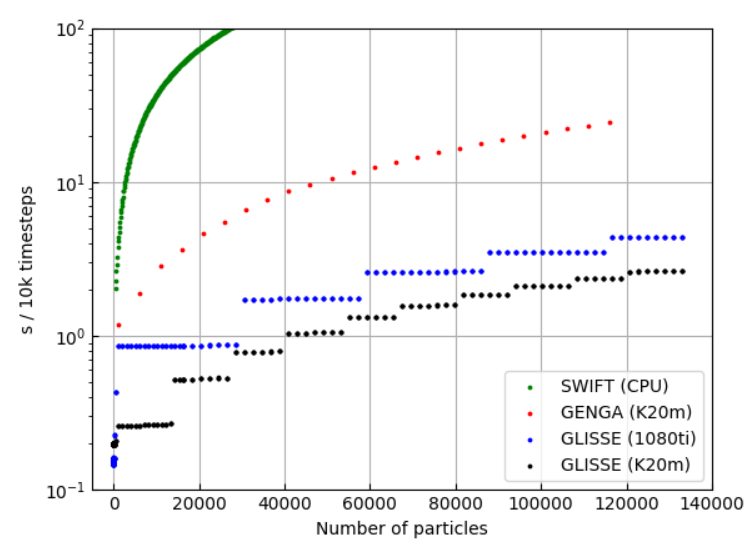
Figure 2: Benchmark simulation duration vs particle count, with 4 massive planets. The CPU-only SWIFT codes show the expected scaling of increasing linearly with number of integrated test particles on this semi-log plot. On the GPUs benchmarked, because of the parallel hardware structure and the software allocation of threads, there is a quantization behavior evident (13,312 particles for the Tesla K20 we dominantly used, and 28,672 for the 1080 Ti GPU). The GPU-code GENGA is more than an order of magnitude faster than the CPU performance (and basically scales linearly in particle number over the entire range) but, on the stability problems studied here, GLISSE’s optimizations provide roughly another order of magnitude speed increase.

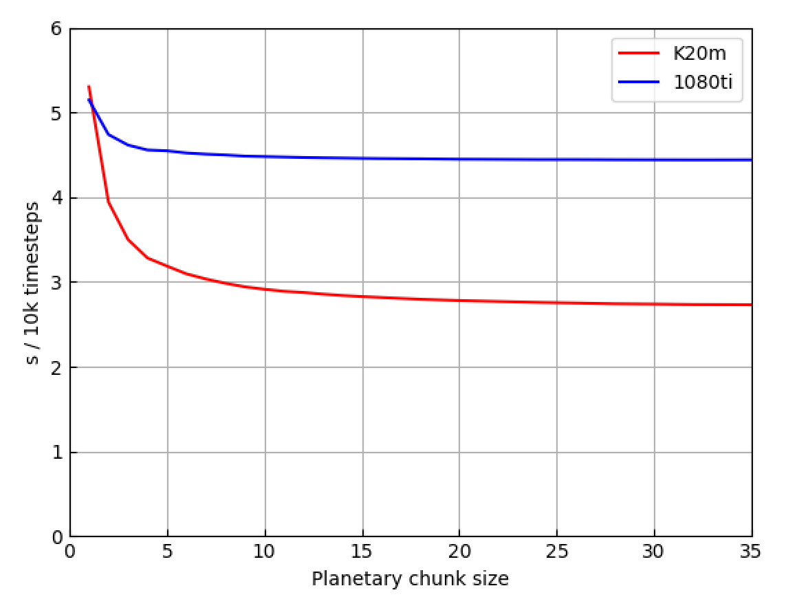
Figure 3: Simulation duration vs planetary chunk size for a simulation with 133120 particles. The speed ratio at a large timeblock size corresponds to the asymptotic speed difference in Figure 2 between the two cards.

2.3 Timing on different CUDA cards

We compared performance of algorithms and hardware using a semirealistic problem of forward computing the orbital evolution of the four giant planets and large numbers of test particles on distant orbits (in integrations short enough that no particles have orbital instability introduced). We recorded the computing time required to advance 10,000 time steps (Figure 2).

We show benchmarks on a conventional graphics card (a NVIDIA 1080ti) and a Kepler K20m GPU unit specifically designed for computation. The hardware characteristics of the CUDA cards will have an obvious influence on the timing. First, the clock speed of the GPU and the number of CUDA cores available on the card control its base speed. In general, a faster clock speed and a higher number of CUDA cores allow a card to perform better. However, unlike many typical GPU applications, planetary dynamics simulations require double-precision floating point arithmetic for satisfactory accuracy. This causes GPU architecture with slow double-precision processors to be penalized, such as in the case of the 1080ti, which actually has a higher number of CUDA cores than the Tesla K20.

Other factors to consider include the number of streaming multiprocessor (SM) units available on the device. As can be seen in Figure 2, execution time is quantized. The quantization is due to automatic software allocation of threads per block; the step size can vary between CUDA versions as the allocation algorithm changes, but the asymptotic speed remains constant. Understanding this behavior allows a user to pick an optimal number of test particles to be performed on each GPU unit. In stability problems where it is expected that there will be rapid early loss of test particles (for example, due to planetary encounters that stop their evolution) the user might start with somewhat more particles than one of the quantization limits; most of the calculation will proceed at the faster pace once enough test particles are discarded.

The GPU clock speed also makes an expected difference. Figure 2 shows that the K20 is overall faster (by factor of up to three, depending on particle number) than the 1080ti. Interestingly, one can observe that at $\simeq$27,000 particles the K20 has just switched over to requiring three quantization groups to cycle through all the test particles, whereas the 1080ti is still able to perform all test particle calculations simultaneously in the first group; for this small range of particle number, the slower clock speed card executes the calculation at nearly the same speed as the K20. In this case, gradual particle removal to a number just less than the quantization step would allow the calculation on the K20 to accelerate.

As an illustration of the optimization introduced by the ‘planetary chunk’ structure, Figure 3 shows the execution time drop caused by delivering planetary logs of various sizes to the GPU (in terms of the number of time steps pre-computed). As can be seen, this improves GLISSE performance on the K20m by a factor of two once 20 or more planetary time steps are pre-computed. (All other results in this paper had this set to a 128$\times dt$ planetary chunk). The performance increase for the 1080ti is only about 10%; we speculate this is because of a faster (PCI 3 versus PCI 2 for the K20m) interface to the motherboard, allowing the 1080ti to push the planet log sufficiently fast to the GPU so that this overhead becomes small.

2.4 Timing vs other methods

Our most basic comparison would be to compare GLISSE’s performance to other integration methods on the same problem but not on a GPU. The GLISSE algorithm we use is very close to the SWIFT [11] package’s implementation of the MVS algorithm. The only major difference for test particle propagation between the SWIFT implementation and GLISSE is the fixed number of iterations for test-particle convergence in GLISSE. In fact, it is likely that SWIFT may use less than 5 iterations to converge for many test particles. Nevertheless, as Figure 2 showed, the SWIFT performance on the CPU is about 100–200 times slower than the same CPU+K20m running GLISSE. The figure also makes it clear that the speed ratio could be a sensitive function of the quantization rate. For the K20m, running 13,312 particles is about 200 times faster than CPU alone, but adding one more particle causes the GPU kernel to repeat the entire kernel for that single test particle, halving the GLISSE speed-up ratio.

We also compared GLISSE’s performance with GENGA [13], an existing GPU-accelerated particle integration package. A general-purpose integrator such as GENGA necessarily includes complex algorithms that allow parallelized processing of particles in close encounters, but the complexities inherent in allowing them to be general purpose sacrifice optimization of the architecture. GLISSE outperforms GENGA on our benchmark, where close encounters do not need to be resolved; Figure 2 shows GENGA to be about 15 times faster than SWIFT, but slower than GLISSE for the test-particle problems we consider here. We achieve this by specializing our code to applications not including close encounters; this allows GLISSE to perform all GPU computations in a single monolithic kernel, which is efficient in GPU memory accesses and CPU/GPU data transfers.

3 Application 1: Stable niches between Uranus and Neptune

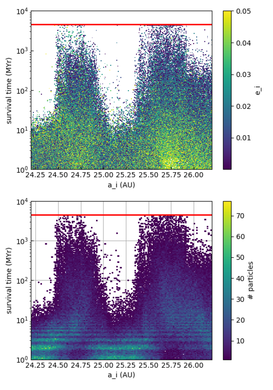
Figure 4: Survival times of particles between Uranus and Neptune, as function of initial semimajor axis $a_{i}$ for the entire $a_{i}$ range studied. Particles are removed upon close approach to a planet. The red line marks the end of the 4.5 Gyr integration. Top: Removals are color coded by initial eccentricity. The trend that the longest living particles are dominated by lower initial eccentricities is obvious. Bottom: Removals are color coded by the number of removals in short bins, illustrating the time-periodic clearing of particles (by Uranus, see text) near the start of the simulation.

The general question of orbital stability for small bodies in planetary systems is an old one. In particular, given the orbits of a set of planets, can one predict on which orbits one could place negligible mass objects upon and have them survive for a given long time scale (or, perhaps, forever)? For a single planet on a circular orbit, a certain orbital separation guarantees (due to the so-called ‘zero velocity curves’ of the circular restricted three-body problem) that the orbit of the particle cannot cross that of the planet [14]. However, there is no general analytic theory for the case of a belt of particles between two planets. In particular, one would like to be able to answer: Given the two planetary masses, how close do the planets need to be before no orbits show stability over some (long) time scale? All successful studies of this type are essentially numerical. For example, Lecar et al. [15] showed that Jupiter and Saturn are sufficiently close that essentially all orbits initially placed between them are unstable on time scales of at most $10^{6}$ yr. Gladman and Duncan [14] used a SIA4 symplectic integrator to show that the zone between Saturn and Uranus is essentially cleared on 30 Myr time scales and that most of the Uranus – Neptune zone is also cleared on 30 Myr time scales except for a region 1-2 au wide near 26 au which showed orbital stability on that time scale. Wisdom and Holman [16] deployed the mixed-variable symplectic map (that we also use here) to confirm complete clearance of the Saturn – Uranus region in much less than the age of the Solar System, as well as directly demonstrating for the first time that the $a\sim 26$ au region could harbour particles for 1 Gyr. Holman pursued this [17] and showed that 0.3% of a test particle population starting with $24<a_{i}<27$ au, $e_{i}<0.01$ and $i_{i}<1^{\circ}$ survived for 4.5 Gyr (although the longest lived particles all had initial semimajor axes near 24.6 and 25.6 au, with dramatically shorter survival times on either side and between these two regions). Thus, given their mass and separation, the Uranus–Neptune pair is not so close as to completely preclude stability over the age of our planetary system. Whether or not we expect bodies to currently be in these stable niches will depend on how strongly initial orbital inclinations and eccentricities of small bodies in this region were excited primordially [17, 18].

Our goal is to better define the region (in $a,e,i$ space) of initial conditions where particles initially between Uranus and Neptune would avoid planetary encounters for 4.5 Gyr of evolution and attempt to diagnose the reason that the borders of the stable region are so well defined. We do this by integrating roughly two orders of magnitude more particles that Holman (1997) was able to, mostly due to the speed increase provided by GLISSE.

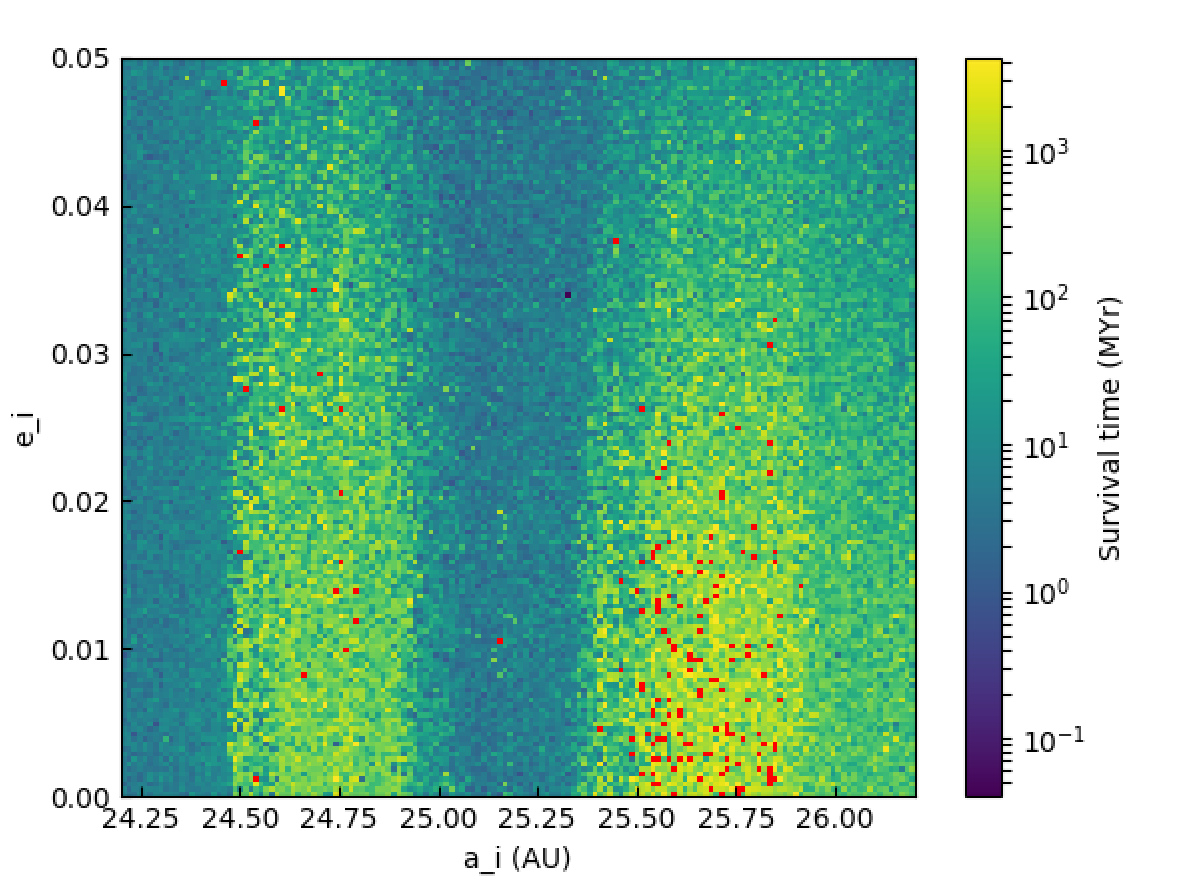
Figure 5: The survival time of particles based on initial semimajor axis $a_{i}$ and initial eccentricity $e_{i}$. Here red dots indicate surviving particles at the end of the 4.5 Gyr integration (which can be mapped to their final values via Figure 6). The very strong instability for $a_{i}$=24.2–24.5 and 24.90–25.35 au is again obvious.

3.1 Initial conditions

We generated 200,000 initial conditions for particles, sampled uniformly over 24.2 au $<a<$ 26.2 au, 0 $<e<$ 0.05, 0 $<i<$ 5^∘ in heliocentric orbital elements. This semimajor axis range covers two-thirds of the 24-27 au interval that [17] originally covered, concentrating for our main integration on only the longest-lived regions. We did also perform smaller preliminary integrations to confirm that no particles outside the $a=$24.2–26.2 au range survived for Gyr time scales; we thus shrank the initial range to obtain a higher density in phase space. Notably, we used larger ranges for $e$ and $i$ than those concluded to be long-term stable [17], as we discovered that some particles within the stable $a$ intervals with somewhat higher eccentricity and/or inclination ($>0.01$ and $>1^{\circ}$, respectively) did in fact survive at least hundreds of millions of years. The preliminary integrations did, however, confirm that all particles above $e>0.05$ and $i>5^{\circ}$ were rapidly unstable in $\ll 1$ Gyr.

A time step of 120 days is short enough to capture the planetary secular frequencies (end of Sec. 2.2) and to detect planetary close approaches given the moderate particle eccentricities achieved. This main 200,000 particle integration took 5 days of continuous computation to run on our K20 GPU. (It should be noted that because many particles are removed quickly, most of the computation occurred with only tens of thousands of particles still surviving). We re-ran the same integration with a time step of 180 days to ensure the accuracy of the simulation; we did not observe any differences in the distribution of surviving particles, and show the results only for the smaller time step computation.

3.2 Simulation results

The gross structure of previous studies was easily reproduced. Figure 4 shows the mix of survival times of the particles as a function of initial semimajor axis $a_{i}$, color-coded by both initial eccentricity $e_{i}$ and by density of particles lost at a given time using a 2D histogram. A very striking aspect of the stability map are the (previously known) sharp semimajor axis boundaries between rapidly unstable and stable particles. For example, particles on either side of $a_{i}=$ 24.50 au have very different stability regimes; those with $a_{i}<24.50$ au are nearly all unstable in $<30$ Myr, while those on the other side of this boundary can last for billions of years (even if some fraction are eliminated in as little as millions of years).

Figure 4b shows that there is a periodicity to the removals that is especially obvious in the first 10 Myr. Investigation revealed that this is clearly due to the fact that the eccentricity of Uranus oscillates with a roughly 1 Myr period, with an amplitude of about 0.07. In contrast, Neptune’s eccentricity always remains factors of several smaller than this. By flagging particles at the time of removal by which planet they encountered, we confirmed that this periodic removal structure is due to Uranus ‘reaching in’ to the region during the high-$e$ phase and encountering (and thus removing) test particles that are at $e\simeq$0.2 at that time. Figure 5 shows the same cube of information as Fig. Figure 4a, but now against initial $a$ and $i$ and highlights (in red) the initial conditions for the particles that are still active at the end of the simulation; within the two most stable bands there is a trend to greater instability with initial eccentricity (again, a feature already known).

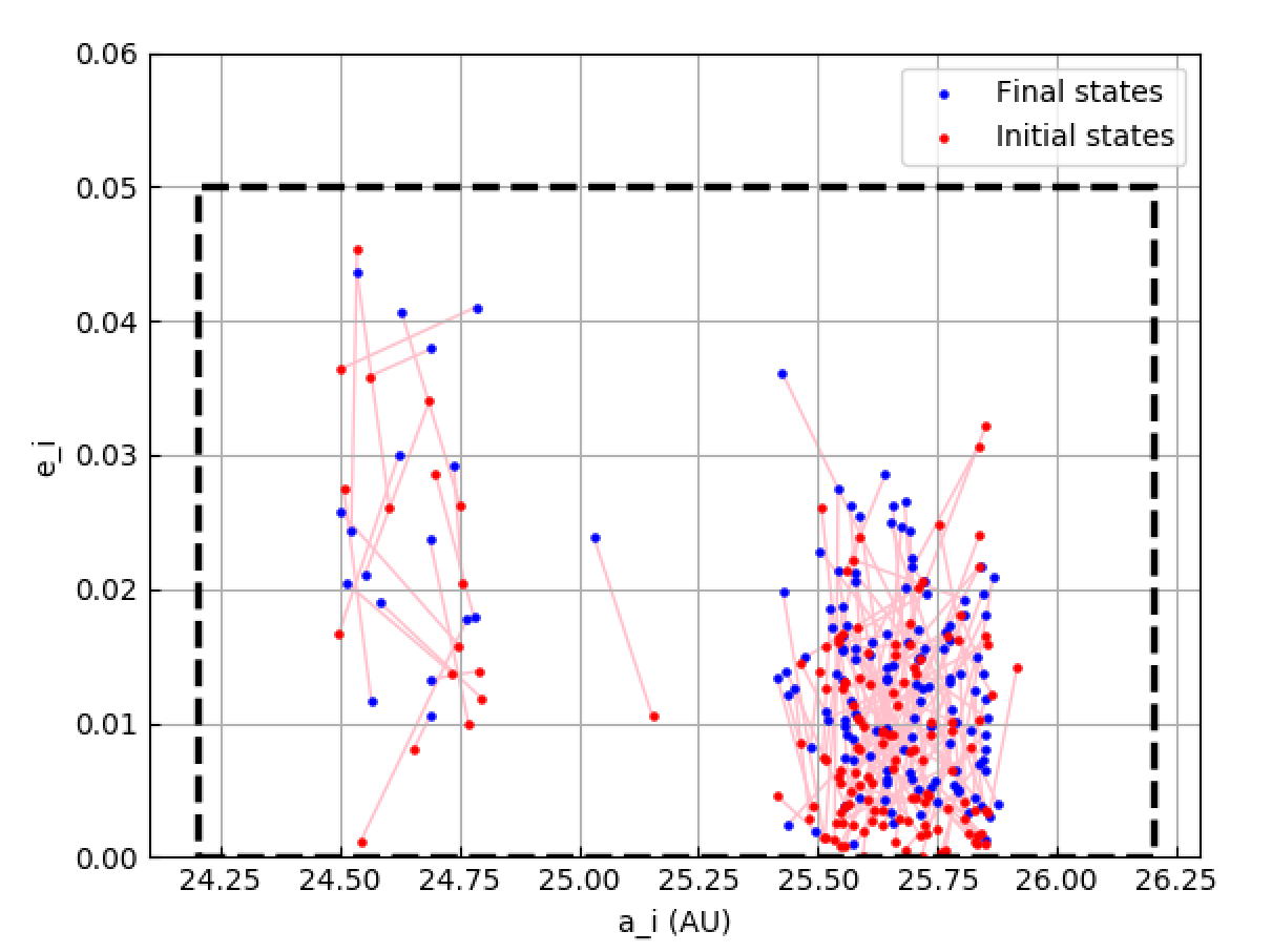
Figure 6: Initial and final orbital elements (connected with a line) for all particles that survive the integration and remain between Uranus and Neptune. (A few particles that manage to scatter to orbits beyond Neptune without ever approaching a planet within 0.5 au are not shown here.) The dashed line represents the boundary of our initial condition set.

How much mobility is there in phase space for particles that survive? In Figure 6, the two main semimajor axis ranges that are stable for 4.5 Gyr are again visible (we observe a single long-lived particle outside of both aforementioned regions, with $a_{i}\approx$ 25.2 au). Perhaps unsurprisingly, particles never migrate between the two stable bands, and the plot also shows that the largest component of the orbital diffusion is a shift in eccentricity, but only on the scale of the $e$ oscillation observed in very short term integrations. That is, the particles that survive are only having their eccentricities moved by a few hundredths over the entire age of the Solar System. The more stable island has almost all its stable particles begin with $e_{i}<0.02$, and those with $e_{i}<0.005$ unsurprisingly ending at eccentricities a factor of roughly 2–4 higher (due to secular oscillations).

3.3 Dynamics of the stability structure

The sharp boundaries of stability seen in Figures 4–6 suggest the presence of some precise dynamical feature as the cause of the instability. Particle removal is almost always marked by an increase in eccentricity, and short-term integration ($\sim 5$ Myr) can provide insight into dynamical behaviour in the system. As a comparison to the complex four-planet system, we also integrated for 4.5 Myr a ‘Uranus+Neptune only’ system, without Jupiter and Saturn; the differences between the 4-planet system proved to be the key to understanding the fine structure.

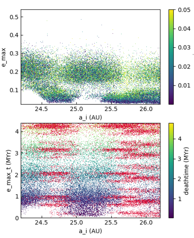
Figure 7: Visualization of maximum eccentricity (and time of maximum eccentricity) achieved by particles over the first 4.5 Myr of a densely time-sampled 4-planet simulation. TOP: Each dot indicated the maximum $e$ reached in 4.5 Myr by each particle with the given initial semimajor axis $a_{i}$, with the color bar showing the initial $e_{i}$. Removed particles are not coded explicitly. BOTTOM: The time at which the $e_{max}$ occurs, with the time of removal codes in the color bar. Red dots indicate particles which survived 4.5 Myr; in vast majority these are the particles with the lowest $e_{max}$ in the upper panel. The banding is due to the periodic $e$ cycling the particles feel with a largest-amplitude period of $\simeq$1 Myr; during one of these cycles the particle gets a slightly higher (but still small) $e$ and this value is the one recorded.

Firstly, we reported above the periodic particle removal due to the $\simeq 1$ Myr eccentricity oscillation of Uranus. Both the time scale and the amplitude are understood by linear secular theory of the planets; Laskar [12] shows that uranian $e$ evolution is dominated by roughly comparable contribution from the secular frequencies $g_{5}$ and $g_{7}$, and the beating between them will produce a maximum amplitude of $\simeq$0.07 with this period. In our integration with Jupiter and Saturn removed, Uranus’ eccentricity oscillated only to a maximum of 0.04, as expected without the extra amplitude provided by $g_{5}$. The 1 Myr period oscillation is thus specific to the four-body problem, and with it, the removal of particles on that period as well. However, this behaviour of Uranus does not explain the fine structure in the stable bands, as we determined that this high-$e$ cycling of Uranus removes particles almost uniformly across the initial semimajor axis range.

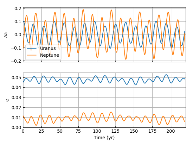
Figure 8: Semimajor axis and eccentricity oscillations (heliocentric elements) of Uranus and Neptune over 200 years in the full four-planet integration. The change in semimajor axis is relative to the 4 Myr average (19.22 au and 30.11 au, respectively). Of critical importance is that the two $\Delta a$’s explore all relative phases, meaning that their mean-motion resonances are shifting (Figure 9) relative to each other.

Secular resonances can destabilize particle orbits by the mechanism of eccentricity pumping if natural precession frequencies match those set by the planetary system. Knezevic et al. [19] used linear secular theory to place two instances of the $g_{6}$ resonance at rough semimajor axes of 24.55 and 25.3 au, for $e=0.1$ and very low inclination, and these are the only secular resonant locations they place in the low-$i$ region of our study. Like Grazier et al. [20], we were unable to find any clear evidence of secular-resonance based eccentricity pumping, despite investing some effort. We examined the detailed eccentricity behaviour in another simulation over several secular timescales (4.5 Myr) in Figure 7. The instability regions do not align with the expected secular locations, and in fact those locations seem to be relatively stable. The number of test particles GLISSE computes allows us to show interesting details of the structure; there are two large contiguous bands of $a_{i}$ where particles can remain at very low $e$ ($<$0.05) for millions of years. Across almost the entire range, however, particles can be raised to $e>0.2$ In addition, the calculation shows that in the region between 24.8 au and 25.6 au, particles are can be raised to planet-crossing $e$ well before the secular eccentricity pumping timescales; in fact, some particles are excited to planet crossing in only 30 kyr.

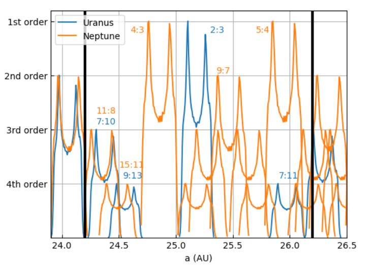
Figure 9: Visualization of the overlap of mean-motion resonances between Uranus and Neptune as the planetary semimajor axes vary. Each curve identifies a particular resonance center ($a$ widths will be of order 0.1 au at these $e$’s), and the vertical coordinate is proportional to the fraction of time (over 4 Myr) that the resonance is at that location (scaled visually to an upper limit denoting resonance order). Note that the locations of the resonances for a single planet always move in lockstep but, because the planetary semimajor axes do not oscillate in phase, particles can see the overlap of a resonance from each planet which clearly leads to rapid strong $e$ excitation. Thick black vertical lines mark the bounds of our initial conditions.

This short time scale means that the most likely explanation relates to mean-motion, rather than secular, resonance. The nominal mean-motion resonance locations due to Uranus and Neptune are well mapped [19, 21], but they do not simply consistently correspond to regions of either stability or instablility. There are three first-order resonances located between 24.2 and 26.2 au: Neptune’s 4:3 near 24.8 au occupies a stabler band near the outer edge of one of Figure 4’s two stability bands. The uranian 2:3 resonance near 25.1 occupies one of the most unstable zones, and Neptune’s 5:4 near 25.9 au straddles the boundary between the most stable region and one of much less stability.

Here our understanding was greatly aided by inspecting the results of the two-planet integration. Overall the region showed greatly increased stability, and regions of eccentricity pumping were more clearly related to the mean-motion resonance locations. Of course, with Jupiter and Saturn gone, the $g_{6}$ secular resonance does not exist so we could not look for this, and no obvious secular resonance existed (even if one could see that the planetary and test particle $e$ oscillations were now dominated by a 2-Myr period present in the Uranus-Neptune pair). The key was to realize that now the two planetary semimajor axes showed more than an order of magnitude less variation, with them being relatively fixed at $19.32\pm 0.01~{}\text{au}$ and $29.98\pm 0.01~{}\text{au}$, respectively. In contrast, in the real planetary system the $e$ evolution driven by 4-planet interaction has enough frequencies that Neptune’s $a$ can be driven $\pm$0.1 au while Uranus is oscillating by 0.2 au, and that these oscillations are not in phase. Thus, while the location of a given planet’s resonances always shift in lock step with the planetary $a$, the relative positions of the uranian and Neptunian resonances can shift by up to 0.3 au (which is more than their typical width at $e<0.1$). This means that the faster-acting mean-motions resonances are continuously moving through resonance overlap, and it became clear that this overlap is what is demarcating the unstable regions.

Figure 9 illustrates the variation of the resonance centers over the first 4 Myr of the 4-planet simulation, with the vertical axis linearly proportional to the time spent at each $a$, and scaled to a vertical maximum defined by the resonance order (with lower-order resonances typically being stronger). The double-peaked character is simply due to more time being spent in a sinusoidal oscillation near the extremes. This figure makes it clear that the rapidly unstable zones correspond to where uranian resonances overlap with those of Neptune, generating dynamical chaos. From 24.90 to 25.35 au the uranian 2:3 overlaps (after accounting for its width) with Neptune’s 4:3, 7:9, 10:13 (centered at 25.25 au), and a 4th order resonance; this range is the rapidly-unstable central valley (Figsures 4, 5, 7). For $a_{i}$=24.2–24.5 au, the uranian 7:10 and the neptunian 11:8 overlap and define the region of rapid instability. It appears the overlap of two 4th order resonances is insufficient to rapidly excite $e$ near 24.6 au. In contrast, Figure 9 shows that in the range $a$=24.5–24.9 and 25.4–25.9 there are only uranian resonances present and we believe this explains the much longer orbital stability times (up to the age of the Solar System) in this region. The uranian 7:11’s overlap near 26 au with Neptune’s 5:4 appears to generate $e$ pumping on only hundreds of Myr (rather than Myr) time scales (Figure 6).

We have shown that this system is highly chaotic and that the stability is not simply described by single-resonance theory. This application shows how GLISSE can provide abundant statistics that permit one to diagnose the resonant behaviour within a very short computation time using GPU acceleration.

4 Application Two: Stability boundaries of external mean-motion resonance with Neptune

In the transneptunian region, resonances often serve the important role of protecting particles from close encounters with Neptune. In fact, the distant resonances still hold a very large total population once debiased for detection effects [22], which rivals the so-called ‘main Kuiper belt’. Although the rough phase space region in which this protection will occur can be estimated via analytic and low-cost numerical methods in the approximation of a single planet (eg. [23]), the long-term dynamical chaos generated by the planets causes portions of the resonance to be gradually eroded over 4 Gyr time scales. (Although there is plausibly an early phase of outward planetesimal-driven migration for Neptune, even the longest-duration estimates over several hundred Myr [24] will still result in $\sim$4 Gyr of dynamical erosion.) A thorough exploration of long-term dynamics of the high-dimensional phase space is thus expensive. We demonstrate how GLISSE can be used in such a context for the 3:1 and 5:2 resonances with Neptune.

4.1 Previous work

The most well-known example of resonance protection is the 3:2 resonance which includes Pluto, first exposed numerically [25]. Note that beyond Neptune much of the literature utilizes the terminology of $m:n$ external resonance numbering with $m>n$ (opposite the terminology we used earlier discussing Uranus and Neptune). Many other transneptunian objects (TNOs) also reside in the 3:2, and as such the structure of this resonance has been heavily studied analytically and numerically [23, 26]. Other resonances with reasonable exploration of the long-term stability of most of the resonant phase space include the 2:1 [27, 28] and the 5:2 [29]. The 3:1 resonance has no similarly rigorous exploration.

Mean motion resonances occur when a particle’s orbital period is a small-integer ratio of a planet’s orbital period. Particles in mean motion resonance have a fast precession of perihelion and are additionally protected from close encounters with the planet due to synchronization of orbital periods, as the particle will reach perihelion (for outer resonances) or aphelion (for inner resonances) when the planet is not nearby.

Particles trapped (librating) in these two resonances can be detected by a restricted variation of the relevant resonant argument:

$$\phi_{31}=3\lambda-\lambda_{N}-2\tilde{\omega}\quad\mathrm{or}\quad\phi_{52}=5\lambda-2\lambda_{N}-3\tilde{\omega}$$

where $\lambda=\tilde{\omega}+M$ is the particle’s mean longitude and $\tilde{\omega}=\Omega+\omega$ its longitude of pericenter, composed of the longitude of ascending node $\Omega$, the argument of perihelion $\omega$, and mean anomaly $M$; $\lambda_{N}$ represents the same quantities for Neptune’s mean longitude. The confinement of $\phi$ values provided by the resonance can generate close-encounter protection from Neptune (see [22] for an introduction), even for planet-crossing particles.

4.2 Long-term stability of the 3:1 resonance

The 3:1 resonance is a distant ($a\simeq 62.6$ au) TNO resonance. There is a strong flux bias towards discovery of the most eccentric members ($e$=0.4–0.5), which are then detected closer than 50 AU despite most of the population at any instant being beyond $d$=70 au from the Sun. After modelling this effect, there must be thousands of $>$100 km diameter objects [22, 30] currently trapped in the resonance, but observationally constraining the existence and distribution of $e<0.4$ members requires deeper surveys. Here we use GLISSE to map the stable phase space to help debiasing observations.

4.2.1 Initial conditions

We generated 200,000 random initial conditions for particles with 61.8 au $<a<$ 63.4 au, 0 $<e<$ 0.7, 0 $<i<$ 50^∘ (in osculating barycentric orbital elements). The angular elements $M,\Omega$, and $\omega$ were distributed uniformly from 0 to 2$\pi$. The randomness of all three angles means that even at the resonance center ($a_{31}=62.6$ au) some particles have angular elements that do not result in libration. This initial box is about 30% larger than the expected $\sim 1$ au width of the resonance at its widest point, but we wished to make sure we covered all possible resonant phase space with our initial hypercube.

We defined librating particles as those with a resonant argument $\phi_{31}$ that never comes within $10^{\circ}$ of $0^{\circ}$ or never within $10^{\circ}$ of $180^{\circ}$. We observed no cases of libration with $\phi_{31}$ centered on zero. Although some particles librate around other angles, the amplitude of libration is low and so the criterion that we use will still correctly identify such particles as librating; in particular, for the 3:1 there are asymmetric librators which librate around $\phi_{31}\simeq 70^{\circ}$ or$290^{\circ}$, like for the 2:1 [22, 28], that are correctly diagnosed due to $\phi$ avoiding zero.

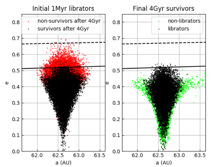
Figure 10: Maps in barycentric $a,e$ space of particles that librate in the 3:1 resonance. The dashed curve indicates Uranus crossing and the solid line Neptune crossing. The initial conditions uniformly filled this $a,e$ space up to $e=0.7$. Left: All particles that librate for the first 1 Myr (that is, at their initial conditions) are plotted. Those which do not survive for 4 Gyr are coded red instead of black. We refer to this as an ‘ice cream cone plot’, for obvious reasons. Right: final states of all initially librating particles (dots in left panel) that are still in this semimajor axis range, with green points indicating particles which do not librate in a 1-Myr extension integration. Black points are plotted on top of red and green points.

4.2.2 Map of stable 3:1 particles

We ran an initial simulation for 1 Myr with a 180-day time step and logged orbital elements at a 2048-year interval. Of the 200,000 initial particles, 10.8% exhibited librating behaviour. As we were interested in the eroding of resonance boundaries over time, we removed all particles that were not librating in the initial integration. With the reduced initial set, we ran a long simulation for 4 Gyr with a 90 day time step to determine long-term behaviour of the remaining 21,610 particles. After this integration, 46% of the initially librating particles were removed due to encounters with Neptune or Uranus. For the remaining particles, we continued the integration for an additional 1 Myr with a 180-day time step to determine which particles were librating at the end of the integration. In the last integration, 8508 particles were librating after 4 Gyr; thus, over half of the initially librating particles were either no longer librating or removed from the integration by 4 Gyr. The $a,e$ values of initially librating particles and their final locations are shown in Figure 10. We were able to reproduce the $\simeq 1$ au initial width of the resonance that Malhotra et al. [29] found, but particles with $e>$0.6 rarely survived even in the initial 1 Myr integration (because the resonance provides no protection against Uranian close encounters) and, less obviously, particles with $e>$0.5 almost never survive the full 4 Gyr integration (Figure 11). This phenomenon shows that despite the possibility in principle of stable Neptune-crossing high-$e$ orbits (like some 3:2 TNOs), the actual gravitational effects from the planets essentially destroy the long-term stability of high-$e$ orbits.

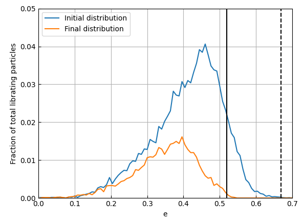
Figure 11: Fractional distribution of the eccentricity of librating 3:1 particles in both the initial 1 Myr integration and again after 4 Gyr have passed. The solid(broken) vertical line represents Neptune(Uranus) crossing at the central resonant semimajor axis. The normalization for both distributions is the 21,610 objects that were initially librating, showing that the relative loss for $e>0.4$ is extremely high over the age of the Solar System.

Figure 10 also shows how the diffusion produces particles that ‘fall out’ of the resonance on either side (mostly large-amplitude librators), some of which then enter the ‘detached’ TNO population (the vast majority of the green points) that only weakly diffuse in $a$ due to small kicks from Neptune near their perihelia. Some diffusion out the sides of the resonance is also visible. At the lowest $e$’s where the resonance is thinnest, the ‘shaking’ of Neptune by the other giant planets also causes particles to drop out of the resonance, leaving nearly no resonant particles with $e<0.10$ in the modern epoch. We show the locations of surviving resonant particles in $(a,i)$ and $(e,i)$ space in Figure 12. Interestingly, the semimajor axies width of the 4-Gyr stable portion of the resonance decreases as the inclination rises, although there are still resonant particles at 50^∘. There is some structure in the $(e,i)$ distribution, with moderate ($\simeq$15–40^∘) orbits being less stable.

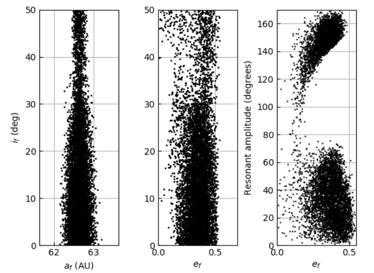
Figure 12: Barycentric osculating orbital elements of surviving particles that at 4 Gyr that still librate in the 3:1 resonance. Notice that the median $e$ rises slightly with inclination until about $i=40^{\circ}$, at which point some nearly circular orbits appear. The libration amplitudes are split into large-amplitude symmetric oscillations and lower-amplitude asymmetric librators (histogrammed in Figure 13).

We performed a simplified analysis to estimate resonant libration amplitudes (the magnitude of variation of $\phi_{31}$ on the time scale of a few resonant librations). We used a running window that diagnosed successive maxima and minima of the resonant angle and measured the difference between them; this simple method provides a rough estimate of the amplitude sufficient for our purposes here. The libration amplitude structure of the 3:1 is as expected (Figures 12 and 13) and similar to the 2:1 resonance [31]; a normal ‘symmetric’ island of large amplitude libration (which we confirmed is centered on $\phi_{31}=180^{\circ}$) and also ‘asymmetric’ librators of amplitudes $<70^{\circ}$ whose resonant angle librates around angles that are in the range 70-90^∘. The two asymmetric islands are equally populated. The symmetric librators have an upper $e$ envelope at each libration amplitude, again similar to the 2:1 [28].

Although we numerically model erosion, it is unlikely that the current 3:1 TNO distribution is as shown here. We will return to this topic after discussing the 5:2 resonance.

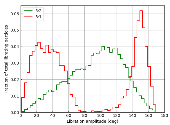
Figure 13: Histogram of our approximate libration amplitudes for the particles that are librating at 4 Gyr, for the 3:1 and the 5:2 resonance. For the 3:1, the large amplitude librations are centered on 180^∘ (right peak) while the lower amplitude librations are the ‘asymmetric librators’.

4.3 Long-term stability of the 5:2 resonance

After accounting for dection bias, the 5:2 and the 3:2 are two of the most heavily-populated resonances in the Kuiper Belt [22]. Due to its larger semimajor axis, fewer 5:2 resonant TNOs are known, it is less well studied than the 3:2 and this makes an empirical understanding of the resonance boundaries even more useful.

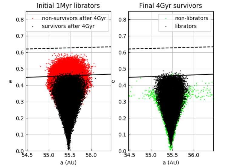
Figure 14: Maps in $a,e$ space of particles that librate in the 5:2 resonance. Curves and dot colors have the same meaning as Figure 10. Left: particles that librate at their initial conditions. Right: Final states of particles shown as black dots on on left.

4.3.1 Previous work

Again, maps of the resonance in phase space by analyzing Poincare sections give a reasonable match to the resonance boundaries over few-Myr time scale [29]. We replicated this result (Figure 14), showing initial 5:2 libration at up to $e\simeq 0.55$. Despite this, the distribution of observed particles shows a cutoff at eccentricities of 0.45 [22, 29, 32], despite detection biases favoring the discovery of higher-$e$ TNOs. It was extremely likely that giant planet perturbations ‘removed the top of the ice cream cone’. GLISSE easily allowed us to explore this with excellent statistics.

4.3.2 Initial conditions and results

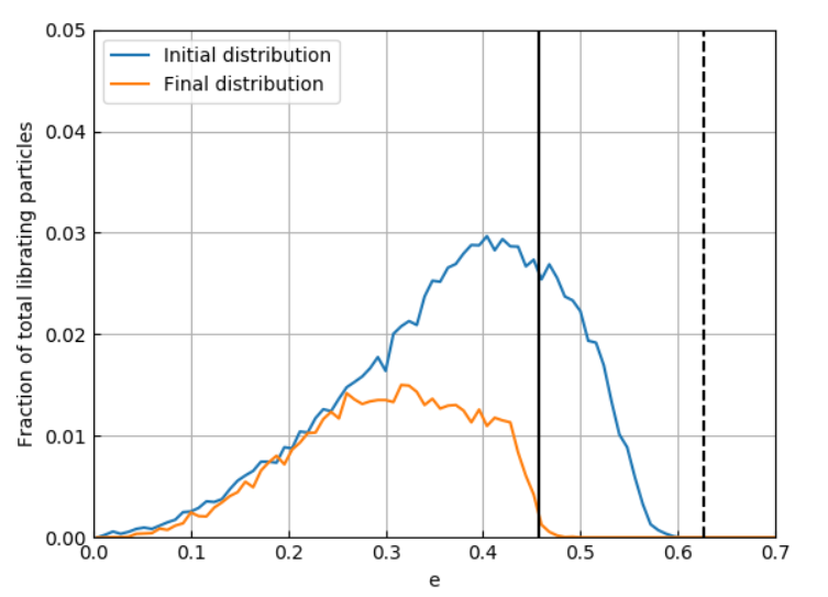
Figure 15: Distribution of the eccentricity of librating 5:2 particles in both the initial integration and the final integration, after 4 GYr has passed. The solid vertical line represents Neptune crossing and the broken vertical line shows Uranus crossing.

We generated 200,000 initial conditions for particles with 54.5 au $<a<$ 56.5 au, 0 $<e<$ 0.7, 1 $<i<$ 20^∘ in osculating barycentric orbital elements. We ran an initial 1 Myr integration with a 180 day time step to find librators, followed by a 4 Gyr integration with a 120 day time step, and then executed another 1 Myr integration with the output particle states from the 4 Gyr integration to find librating particles at the end state. Malhotra et al. [29] speculated that long-term erosion on solar system time scales would remove the population with $e>0.45$. Our GLISSE simulations (Figure 15) easily show this to be true, truncating the survivors at this eccentricity (which is the highest of the known 5:2 librators), while also demonstrating major loss over the solar system age for $e>0.25$. There are again particles which diffuse out of the resonance over the 4 Gyr and are found either just beyond the borders at low $e$ or in the detached population on either side with $e\approx 0.35$. Curiously, this integration exhibits slightly more objects on the low-$a$ side of the resonance; if not chance, this might influence conclusions related to this asymmetry being caused by dropouts during the final stages of planetary migration [33].

Figure 16 shows the orbital element distribution (at 4 Gyr) of the survivors. Unlike the 3:1, there is no obvious inclination dependence of the survivors over the explored range, although we initially only used $i_{o}$=1–20^∘ in this study and can see the diffusion of up to 7 degrees higher over the age of the Solar System. The stable libration amplitudes are (like the 3:2 resonance) all centered symmetrically on 180^∘, with a resonance libration amplitude distribution (at 4 Gyr) shown in Figure 13, which is very similar to that derived for the 3:2 [22].

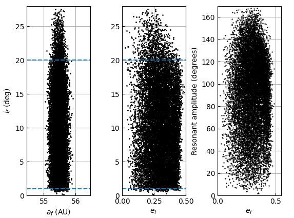
Figure 16: Barycentric orbital elements of test particles that survive 4 Gyr of evolution and at that point still librate in the 5:2 resonance over an additional short 1 Myr integration. Note that no there were no initial conditions with $i_{o}<1^{\circ}$ or $i_{o}>20^{\circ}$ (dashed horizontal lines).

4.4 Comparison Considerations

Although GLISSE has allowed us to create a well-sampled 4 Gyr stability survey of the two resonances, it is unlikely to be a perfect representation of the current TNO distribution. Only if somehow the early Solar System ‘uniformly filled’ the phase space would our final map be accurate. Instead, it is most plausible that many TNOs were initially introduced into the resonance via resonant capture of existing TNOs or from the Neptune-coupled scattering population during planetary migration. These mechanisms are unlikely to fill the resonance uniformly like we have done for this numerical survey. In addition, in the more recent past, objects in the scattering population will temporarily ‘stick’ to the resonances, forming a metastable population [34] which will mostly have higher eccentricities and libration amplitudes than primordial populations. This makes quantitative comparison of the current object set even more complicated than just the problem of observational bias [33, 35].

5 Conclusions and Future Perspectives

We have demonstrated the design and utility of a large-scale particle integrator. In particular, we have shown that thoughtful design of algorithms using Graphics Processing Units (GPUs) can bring improvements in speed of one hundred times over existing CPU integrators such as SWIFT. GLISSE can pave the road for more detailed examinations of Solar System dynamics, in particular, in examining the stability of hundreds of thousands of orbits over billions of years. It is natural to consider as a next step the investigation of orbit evolution when some close encounters with planets are considered. Close encounter handling is inherently a non-parallel process and thus it will be better to have GLISSE resolve particle close encounters on the CPU. Moving the few particles in rare close encounters off the GPU will allow the bulk of particles not in close encounters to continue to be integrated at optimal speeds without being limited by factors such as branch divergence mentioned in section 2. Our intention is to work towards such a close-encounter capable algorithm.

Appendix A Acknowledgements

We thank the National Sciences and Research Council of Canada for research and salary support, and Samantha Lawler for useful comments.

Declarations of interest: none.

References

- [1] D. Groen, S. Portegies Zwart, S. McMillan, J. Makino, Distributed N-body simulation on the grid using dedicated hardware, New A13 (5) (2008) 348–358. arXiv:0709.4552, doi:10.1016/j.newast.2007.11.004.
-
[2]
M. Abadi, P. Barham, J. Chen, Z. Chen, A. Davis, J. Dean, M. Devin,
S. Ghemawat, G. Irving, M. Isard, M. Kudlur, J. Levenberg, R. Monga,
S. Moore, D. G. Murray, B. Steiner, P. A. Tucker, V. Vasudevan, P. Warden,
M. Wicke, Y. Yu, X. Zhang, Tensorflow:
A system for large-scale machine learning, CoRR abs/1605.08695.
arXiv:1605.08695.
URL http://arxiv.org/abs/1605.08695 -
[3]
I. Buck, T. Foley, D. Horn, J. Sugerman, K. Fatahalian, M. Houston,
P. Hanrahan, Brook for
gpus: Stream computing on graphics hardware, in: ACM SIGGRAPH 2004 Papers,
SIGGRAPH ’04, ACM, New York, NY, USA, 2004, pp. 777–786.
doi:10.1145/1186562.1015800.
URL http://doi.acm.org/10.1145/1186562.1015800 - [4] E. B. Ford, Parallel algorithm for solving kepler’s equation on graphics processing units: Application to analysis of doppler exoplanet searches, New Astron.arXiv:arXiv:0812.2976, doi:10.1016/j.newast.2008.12.001.
-
[5]
S. Dindar, E. B. Ford, M. Juric, Y. I. Yeo, J. Gao, A. C. Boley, B. Nelson,
J. Peters,
Swarm-ng:
A cuda library for parallel n-body integrations with focus on simulations of
planetary systems, New Astronomy 23-24 (2013) 6 – 18.
doi:https://doi.org/10.1016/j.newast.2013.01.002.
URL http://www.sciencedirect.com/science/article/pii/S1384107613000092 -
[6]
P. Sharp, W. Newman,
Gpu-enabled
n-body simulations of the solar system using a vovs adams integrator,
Journal of Computational Science 16 (2016) 89 – 97.
doi:https://doi.org/10.1016/j.jocs.2016.04.003.
URL http://www.sciencedirect.com/science/article/pii/S1877750316300412 - [7] A. Moore, A. C. Quillen, QYMSYM: A GPU-accelerated hybrid symplectic integrator that permits close encounters, New A16 (7) (2011) 445–455. arXiv:1007.3458, doi:10.1016/j.newast.2011.03.009.
-
[8]
G. Ogiya, M. Mori, Y. Miki, T. Boku, N. Nakasato,
Studying the
core-cusp problem in cold dark matter halos usingN-body simulations on
GPU clusters, Journal of Physics: Conference Series 454 (2013) 012014.
doi:10.1088/1742-6596/454/1/012014.
URL https://doi.org/10.1088%2F1742-6596%2F454%2F1%2F012014 -
[9]
Jalali, B., Baumgardt, H., Kissler-Patig, M., Gebhardt, K., Noyola,
E., Lützgendorf, N., de Zeeuw, P. T.,
A dynamical n-body model
for the central region of tauri, A&A 538 (2012) A19.
doi:10.1051/0004-6361/201116923.
URL https://doi.org/10.1051/0004-6361/201116923 - [10] J. Wisdom, M. Holman, Symplectic maps for the n-body problem, Astron. J 102 (1991) 1528–1538. doi:10.1086/115978.
- [11] H. F. Levison, M. J. Duncan, The Long-Term Dynamical Behavior of Short-Period Comets, Icarus108 (1) (1994) 18–36. doi:10.1006/icar.1994.1039.
- [12] J. Laskar, Secular evolution of the solar system over 10 million years, A&A198 (1988) 341–362.
-
[13]
S. L. Grimm, J. G. Stadel,
The genga code:
Gravitational encounters in n-body simulations with gpu acceleration, The
Astrophysical Journal 796 (1) (2014) 23.
doi:10.1088/0004-637x/796/1/23.
URL https://doi.org/10.1088%2F0004-637x%2F796%2F1%2F23 - [14] B. Gladman, M. Duncan, On the fates of minor bodies in the outer solar system, AJ100 (1990) 1680–1693. doi:10.1086/115628.
- [15] F. Franklin, M. Lecar, P. Soper, On the original distribution of the asteroids. II - Do stable orbits exist between Jupiter and Saturn?, Icarus79 (1989) 223–227. doi:10.1016/0019-1035(89)90118-8.
- [16] M. J. Holman, J. Wisdom, Dynamical stability in the outer solar system and the delivery of short period comets, AJ105 (1993) 1987–1999. doi:10.1086/116574.
- [17] M. J. Holman, A possible long-lived belt of objects between Uranus and Neptune, Nature387 (1997) 785–788.
- [18] A. Brunini, M. D. Melita, On the Existence of a Primordial Cometary Belt between Uranus and Neptune, Icarus135 (1998) 408–414. doi:10.1006/icar.1998.5992.
- [19] Z. Knezevic, A. Milani, P. Farinella, C. Froeschle, C. Froeschle, Secular resonances from 2 to 50 AU, Icarus93 (2) (1991) 316–330. doi:10.1016/0019-1035(91)90215-F.
- [20] K. R. Grazier, W. I. Newman, F. Varadi, W. M. Kaula, J. M. Hyman, Dynamical Evolution of Planetesimals in the Outer Solar System. II. The Saturn/Uranus and Uranus/Neptune Zones, Icarus140 (2) (1999) 353–368. doi:10.1006/icar.1999.6147.
- [21] T. Gallardo, Atlas of the mean motion resonances in the Solar System, Icarus184 (1) (2006) 29–38. doi:10.1016/j.icarus.2006.04.001.
- [22] B. Gladman, S. M. Lawler, J. M. Petit, J. Kavelaars, R. L. Jones, J. W. Parker, C. Van Laerhoven, P. Nicholson, P. Rousselot, A. Bieryla, M. L. N. Ashby, The Resonant Trans-Neptunian Populations, AJ144 (1) (2012) 23. arXiv:1205.7065, doi:10.1088/0004-6256/144/1/23.
- [23] R. Malhotra, The Phase Space Structure Near Neptune Resonances in the Kuiper Belt, AJ111 (1996) 504. arXiv:astro-ph/9509141, doi:10.1086/117802.
- [24] D. Nesvorný, Dynamical Evolution of the Early Solar System, ARA&A56 (2018) 137–174. arXiv:1807.06647, doi:10.1146/annurev-astro-081817-052028.
- [25] C. J. Cohen, E. C. Hubbard, Libration of the close approaches of Pluto to Neptune, AJ70 (1965) 10. doi:10.1086/109674.
- [26] A. Morbidelli, Chaotic Diffusion and the Origin of Comets from the 2/3 Resonance in the Kuiper Belt, Icarus127 (1) (1997) 1–12. doi:10.1006/icar.1997.5681.
- [27] M. S. Tiscareno, R. Malhotra, Chaotic Diffusion of Resonant Kuiper Belt Objects, AJ138 (3) (2009) 827–837. arXiv:0807.2835, doi:10.1088/0004-6256/138/3/827.
- [28] Y.-T. Chen, B. Gladman, K. Volk, R. Murray-Clay, M. J. Lehner, J. J. Kavelaars, S.-Y. Wang, H.-W. Lin, P. S. Lykawka, M. Alexandersen, M. T. Bannister, S. M. Lawler, R. I. Dawson, S. Greenstreet, S. D. J. Gwyn, J.-M. Petit, OSSOS. XVIII. Constraining Migration Models with the 2:1 Resonance Using the Outer Solar System Origins Survey, AJ158 (5) (2019) 214. arXiv:1910.12985, doi:10.3847/1538-3881/ab480b.
- [29] R. Malhotra, L. Lan, K. Volk, X. Wang, Neptune’s 5:2 Resonance in the Kuiper Belt, AJ156 (2018) 55. arXiv:1804.01209, doi:10.3847/1538-3881/aac9c3.
- [30] M. Alexandersen, B. Gladman, J. J. Kavelaars, J.-M. Petit, S. D. J. Gwyn, C. J. Shankman, R. E. Pike, A Carefully Characterized and Tracked Trans-Neptunian Survey: The Size distribution of the Plutinos and the Number of Neptunian Trojans, AJ152 (5) (2016) 111. arXiv:1411.7953, doi:10.3847/0004-6256/152/5/111.
- [31] E. I. Chiang, A. Jordan, On the Plutinos and Twotinos of the Kuiper Belt, Astron. J. 124 (2002) 3430. arXiv:astro-ph/0210440, doi:10.1086/344605.
-
[32]
K. Volk, R. Murray-Clay, B. Gladman, S. Lawler, M. T. Bannister, J. J.
Kavelaars, J.-M. Petit, S. Gwyn, M. Alexandersen, Y.-T. Chen, P. S. Lykawka,
W. Ip, H. W. Lin,
OSSOS
III—RESONANT TRANS-NEPTUNIAN POPULATIONS: CONSTRAINTS
FROM THE FIRST QUARTER OF THE OUTER SOLAR SYSTEM ORIGINS
SURVEY, The Astronomical Journal 152 (1) (2017) 23.
doi:10.3847/0004-6256/152/1/23.
URL https://doi.org/10.3847%2F0004-6256%2F152%2F1%2F23 - [33] S. M. Lawler, R. E. Pike, N. Kaib, M. Alexandersen, M. T. Bannister, Y. T. Chen, B. Gladman, S. Gwyn, J. J. Kavelaars, J. M. Petit, K. Volk, OSSOS. XIII. Fossilized Resonant Dropouts Tentatively Confirm Neptune’s Migration Was Grainy and Slow, AJ157 (6) (2019) 253. arXiv:1808.02618, doi:10.3847/1538-3881/ab1c4c.
-
[34]
T. Y. M. Yu, R. Murray-Clay, K. Volk,
Trans-neptunian objects
transiently stuck in neptune’s mean-motion resonances: Numerical simulations
of the current population, The Astronomical Journal 156 (1) (2018) 33.
doi:10.3847/1538-3881/aac6cd.
URL https://doi.org/10.3847%2F1538-3881%2Faac6cd - [35] R. E. Pike, S. M. Lawler, Details of Resonant Structures within a Nice Model Kuiper Belt: Predictions for High-perihelion TNO Detections, AJ154 (4) (2017) 171. arXiv:1709.03699, doi:10.3847/1538-3881/aa8b65.