Improving the Line of Sight for the Anisotropic 3-Point Correlation Function of Galaxies: Centroid and Unit-Vector-Average Methods Scaling as $\mathcal{O}(N^{2})$

Abstract

The 3-Point Correlation Function (3PCF), which measures correlations between triplets of galaxies, is a powerful tool for the current era of high-data volume, high-precision cosmology. It goes beyond the Gaussian cosmological perturbations probed by the 2-point correlation function, and includes late-time non-Gaussianities introduced by both nonlinear density field evolution and galaxy formation. The 3PCF also encodes information about peculiar velocities, which distort the observed positions of galaxies along the line of sight away from their true positions. To access this information, we must track the 3PCF’s dependence not only on each triangle’s shape, but also on its orientation with respect to the line of sight. Consequently, different choices for the line of sight will affect the measured 3PCF. Up to now, the line of sight has been taken as the direction to a single triplet member (STM), but which triplet member is used impacts the 3PCF by $\sim$20% of the statistical error for a BOSS-like survey. For DESI (2019-24), which is 5$\times$ more precise, this would translate to $\sim$100% of the statistical error, increasing the $total$ error bar by $\sim$40%. We here propose a new method that is fully symmetric between the triplet members, and uses either the average of the three galaxy position vectors (which we show points to the triangle centroid), or the average of their unit (direction) vectors. We prove that these two methods are equivalent to $\mathcal{O}(\theta^{2})$, where $\theta$ is the angle subtended at the observer by any triangle side. Naively, these approaches would seem to require triplet counting, scaling as $N^{3}$, with $N$ the number of objects in the survey. By harnessing the solid harmonic shift theorem, we here show how these methods can be evaluated scaling as $N^{2}$. We expect that they can be used to make a robust, systematics-free measurement of the anisotropic 3PCF of upcoming redshift surveys such as DESI. So doing will in turn open an additional channel to constrain the growth rate of structure and thereby learn the matter density as well as test the theory of gravity.

1 Introduction

During the first $10^{-35}$ seconds, the universe experienced a period of exponential expansion known as inflation. The field driving this then decayed into radiation and matter, producing density fluctuations standardly taken to be a Gaussian Random Field (GRF). For a GRF, the 2-point correlation function (2PCF), measuring the excess probability over random of finding a pair of points with given density fluctuations separated by a given distance, captures all the information. However, over the Universe’s subsequent evolution, gravitational interactions led to nonlinear structure formation, inducing additional correlation in the density fluctuation field. Hence this field began to deviate from a GRF, and higher-order correlation functions arose. In particular, nonlinear evolution of matter under gravity produces a 3-Point Correlation Function (3PCF) for the matter, where the 3PCF characterizes the excess probability over random of observing three density fluctuation values on a given triangle configuration (e.g. Bernardeau et al. 2002). Furthermore, galaxies do not perfectly trace the matter (galaxy biasing, e.g. Desjacques et al. 2018), which induces additional higher-order correlations, including contributions to the 3PCF (e.g. Gaztanaga 1994, Jing & Borner 2004, Guo et al. 2015, and Slepian & Eisenstein 2017; also see e.g. Scoccimarro et al. 1999 or Gil-Marín et al. 2015 for discussion of biasing in the 3PCF’s Fourier space analog the bispectrum).

Since the 3PCF stems from both nonlinear matter evolution and galaxy biasing, on large scales it can be used in conjunction with the 2PCF to disentangle matter clustering from galaxy bias. It can also be used to investigate in more detail how galaxies trace the matter, since it is sensitive to more complicated models of galaxy biasing (e.g. scaling as the matter field squared, or as the matter field’s tidal tensor (McDonald & Roy, 2009; Chan et al., 2012), or as the baryon-dark matter relative velocity (Yoo et al., 2011; Slepian & Eisenstein, 2015c; Slepian et al., 2018)) at leading order, in contrast to the 2PCF which contains these terms only at sub-leading order. On even larger scales, the 3PCF contains Baryon Acoustic Oscillations (BAO) and so measuring it can offer a standard ruler by which to gauge the cosmic expansion history and in turn constrain dark energy (Slepian et al., 2017); for the analogous method using the bispectrum see Pearson & Samushia (2018).

However, as is true for the 2PCF as well, the 3PCF is affected by the fact that galaxies’ true, 3D positions are unknown. Their peculiar velocities introduce a component to the observed redshift beyond what would come from co-movement with the background expansion alone. This in turn affects the distance inferred for the galaxy. The distortions induced by these velocities on the observed map of 3D galaxy positions are termed Redshift-Space Distortions (RSD).

Physically, the peculiar velocities producing RSD stem from two factors:

1. the large-scale density field, in which potential wells attract galaxies, and make them appear bluer when their additional recessional velocity is pointing to the observer, and redder when it points away from them. The galaxy distribution appears squashed along the line of sight due to this effect, referred as the Kaiser effect (Kaiser, 1987); and

2. the motion of satellite galaxies within clusters, which cause random motions on galaxies in smaller scales. Since in this case the velocities are random inside the clusters, and we only measure the radial contribution, structures on cluster scales will seem to have an elongated shape, referred to as Fingers of God (FOG; Jackson 1972).

No model for the redshift-space 3PCF including both of these effects yet exists, though a number of works investigate RSD in the bispectrum, the 3PCF’s Fourier-space analog. Scoccimarro et al. (1999) uses Eulerian Standard Perturbation Theory (SPT) and incorporates effect (i), and Rampf & Wong (2012) use Lagrangian Perturbation Theory (LPT) and include re-summed contributions which correspond to higher-order SPT terms in the redshift-space bispectrum, but the RSD treatment still includes just (i). Developments of the Scoccimarro et al. (1999) model by Gil-Marín et al. (2015) also include effect (ii), and this model was further extended to the case of Primordial Non-Gaussianity (PNG) by Tellarini et al. (2016).

While some of the above models characterize the dependence of the bispectrum on the triangle’s orientation with respect to the line of sight (e.g. Scoccimarro et al. 1999, Rampf & Wong 2012), there have been only a very few works showing how to measure the anisotropic bispectrum or 3PCF; we discuss those that exist in §2. Yet the time is ripe for further developing such algorithms. Using an algorithm presented in the same work, Sugiyama et al. (2018) recently reported the first evidence for an anisotropic signal in the 3PCF’s Fourier-space analog, the bispectrum, and using mock catalogs, Sugiyama et al. (2020) investigated self-consistent fitting of the anisotropic 2PCF and anisotropic 3PCF. Moreover, a spate of recent works have forecast that measuring anisotropic bispectrum of 3PCF offers significant gains on cosmological parameters. Gagrani & Samushia (2017) forecasts that anisotropic bispectrum offers a factor of 3 improvement on the logarithmic growth rate $f$ relative to 2PCF alone. Even if we treat linear bias and the clustering normalization ($\sigma_{8}$) as fully unknown (a highly conservative choice), Gualdi & Verde (2020) forecasts that 3PCF offers a 30% improvement over 2PCF alone on each of these parameters (including $f$). Thus, measuring the anisotropic 3PCF, and doing so with both high accuracy and high precision, is an important way to extend the reach of upcoming surveys such as Dark Energy Spectroscopic Instrument (DESI; Levi et al. 2019).

However, the line of sight used to a given triplet of galaxies is an important piece of any such effort. All previous works have used the line of sight as given by one of the three triplet members, as discussed in more detail in §2. We term this approach “single-triplet member,” or STM for short. However, Sugiyama et al. (2018) shows that the anisotropic bispectrum changes by as much as 20% relative to its statistical errorbars as one cycles from using one galaxy as the line of sight to another to the third. This work was done for a Sloan Digital Sky Survey (SDSS) Baryon Oscillation Spectroscopic Survey (BOSS)-like sample, and the contribution of such an error would be only a 2% increase in the total error budget. However, DESI will have roughly 5$\times$ the precision of BOSS, and hence a 20% effect relative to BOSS’s statistical errorbars would be a 100% one relative to DESI’s. Thus, the change as one shifts from one galaxy to another in a triplet to define the line of sight would inflate DESI’s anisotropic bispectrum errorbars by as much as a factor of $\sqrt{2}$, meaning a 40% increase in the total error budget. While one might think that averaging over the three choices for line of sight on each galaxy triplet would cause some of this error to cancel, much as happens for the anisotropic 2PCF when the line of sight is taken to be a single galaxy pair member (see Slepian & Eisenstein 2015a for reasons) we further outline in §2, this cancellation does not occur.

Hence, it is worth considering if an estimator that uses a more symmetric definition of the line of sight to a triangle (rather than just choosing one triangle member at a time) can be developed. Furthermore, given the typical computational expense of 3PCF, it is worth seeking an estimator that harnesses the algorithmic innovations of Slepian & Eisenstein (2015d), Slepian & Eisenstein (2018) or Sugiyama et al. (2018), all of which exploit spherical harmonics to factorize the 3PCF or bispectrum calculations. Scoccimarro (2015) also has a fast algorithm but, as we will detail further in §2, it does not capture the full anisotropic information.

In this work, we develop a fully symmetric approach to defining the line of sight to a galaxy triplet. We investigate two choices: first, a straight average of the three absolute position vectors of the galaxies in the observer’s frame, and second, an average of their direction vectors (i.e. make each position vector into a unit vector) in the observer’s frame. We prove that the first choice actually passes through the centroid of the triangle, and hence term that method the “centroid method.” We term the second method the "unit-vector average" method. We also show that these two choices differ from each other only at $\mathcal{O}(\theta^{2})$, where $\theta$ is the ratio of the typical triangle side to the distance of the triangle from the observer. $\theta$ is essentially the angle each side subtends at the observer, and for small $\theta$, we are in the flat sky limit. We note that both the above choices of lines of sight are fully symmetric under interchange of the triplet members with each other, unlike the “single-triplet member” estimators previously used.

Most critically, in this work we show how the anisotropic 3PCF using the above definitions of the line sight can be evaluated scaling as $N^{2}$, where $N$ is the number of objects in the survey. To do so, we exploit the Solid Harmonic Shift Theorem to develop a series expansion for spherical harmonics of our line of sight in terms of spherical harmonics of each triplet member’s position vector. Our expressions give the exact result for evaluating these improved lines of sight to arbitrary precision. However, the computational cost does rise slightly. Nonetheless, to obtain the leading-order correction that goes beyond STM requires only a very modest increase in computational work. We present explicit expressions for the leading-order correction terms needed.

This paper is laid out as follows. In §2 we summarize previous algorithms for the anisotropic 3PCF and bispectrum. In §3 we present the basis used in this work. In §4 we discuss our choices of line of sight and prove both that the average of position vectors gives the triangle centroid, and that this method and the unit-vector-average method agree at $\mathcal{O}(\theta^{2})$. In §5 we show how to evaluate our basis in a factorized fashion that permits an $\mathcal{O}(N^{2})$ scaling. §6 gives explicit expressions for the leading-order terms required by our method to go beyond STM. §LABEL:sec:conclusions concludes. In Appendix LABEL:app:app1 we derive the core expansions, of spherical harmonics of a sum of vectors into spherical harmonics of single vectors, that this work harnesses. This uses the solid harmonic addition theorem, and to offer the reader some intuition on this useful mathematical result, in Appendix LABEL:app:app2 we provide an explicit proof of the low-$\ell$ cases of the theorem using Cartesian forms of the spherical harmonics. Finally, in Appendix C we show how to turn a product of spherical harmonics of the same argument into a sum over single harmonics, a result we require in the work.

2 Previous Work on the Anisotropic Bispectrum and 3PCF

We here outline three previous approaches to the anisotropic bispectrum and 3PCF. In this work, we build on the third of these approaches. The second is actually exactly equivalent to the third in terms of the means of evaluating; the bases of the second and third are simply related by a linear transformation. Our discussion of the first is for the sake of completeness, and to fully explore the issue of how rotating among the three triplet members to define the line of sight enters previous methods.

2.1 Scoccimarro

We here discuss three previous works that presented algorithms for computing the anisotropic 3PCF or bispectrum. First, Scoccimarro (2015) developed a method to obtain multipole moments of the bispectrum. We first briefly articulate the parametrization used in that work, as understanding it is necessary to then follow its treatment of the line of sight, denoted $\hat{n}$. Scoccimarro (2015) parameterizes the bispectrum by the angle cosine $\mu\equiv\hat{k}_{1}\cdot\hat{n}$ of the largest wave-vector, defined to be $\vec{k}_{1}$, to the line of sight. A further parameter is the azimuthal angle $\omega$ of the second-largest, defined to be $\vec{k}_{2}$, about $\vec{k}_{1}$. This parametrization is necessary because, at fixed internal triangle angle, the orientation of $\vec{k}_{2}$ is not fully independent from that of $\vec{k}_{1}$. At fixed $\mu\equiv\hat{k}_{1}\cdot\hat{n}$, $\vec{k}_{1}$ lives on a cone about the line of sight, and at fixed $\vec{k}_{1}$, $\vec{k}_{2}$ lives on a cone about $\vec{k}_{1}$ with opening angle cosine $\hat{k}_{1}\cdot\hat{k}_{2}$.

To parametrize the triangle itself, Scoccimarro (2015) then uses $k_{1},k_{2},k_{3}$, the three triangle side-lengths in Fourier space. These fully characterize the triangle; we term them “internal” parameters, and term $\mu$ and $\omega$ “external.” Scoccimarro (2015) then averages over rotations of $\vec{k}_{2}$ about $\vec{k}_{1}$, reducing the anisotropic bispectrum to a 4D function of $k_{1},k_{2},k_{3}$ and $\mu$ whose $\mu$-dependence can then be expanded in Legendre polynomials. That work then bins the bispectrum by $k_{1},k_{2},k_{3}$. On each such bin, it records multipoles $\ell=0$ and $2$ with respect to $\mu$.

In detail, this is done by taking a “local” bispectrum estimate about a point $\vec{x}$, initially taken to be the centroid of a triangle formed by three galaxies in configuration space. Hence, the bispectrum is formed as an average over contributions taken on a galaxy-triplet-by-galaxy-triplet-basis. One then averages over all triplets by integrating over $\vec{x}$. Scoccimarro (2015) suggests using $\vec{x}$ as defining the line of sight to the galaxy triplet, and forming multipoles with respect to $\hat{k}_{1}\cdot\hat{x}$. To accelerate the estimator, Scoccimarro (2015) then replaces $\vec{x}$ with $\vec{x}_{i}$ , where $\vec{x}_{i}$ is the position vector of a single triplet member. Consequently, we term this a “‘single triplet member” (STM) method.

Overall, each galaxy triplet will contribute to a given $k_{1},k_{2},k_{3}$ bin three times: once with $\hat{x}_{1}$, once with $\hat{x}_{2}$, and once with $\hat{x}_{3}$ as the line of sight for the multipoles. This point is important because it connects to the analogous procedure for the anisotropic 2PCF, known as the “single pair member” (SPM) line of sight or the “Yamamoto approximation” (Yamamoto et al., 2006). This method for the 2PCF results in cancellation of the difference between it and the angle bisector or separation midpoint (for the 2PCF) up to order $\theta^{2}$ (Slepian & Eisenstein, 2015b). $\theta$ is the opening angle of the triangle formed by the observer and the galaxy pair. In particular, for the 2PCF, this cancellation occurs because each galaxy pair contributes twice to whatever separation bin it enters, once with each pair member’s position defining the line of sight. The fact that the Scoccimarro (2015) approach allows each triplet member to define the line of sight in turn and co-add into one $k_{1},k_{2},k_{3}$ bin might suggest that an analogous cancellation to that in the 2PCF applies. Specifically, we might ask if the Scoccimarro (2015) STM method agrees with using the line of sight to e.g. the triangle centroid up to $\mathcal{O}(\theta^{2})$. However, we have not been able to prove such a result.

2.2 Slepian & Eisenstein

Slepian & Eisenstein (2018) presented a method to compute the spherical harmonic decomposition of the anisotropic 3PCF scaling as $N^{2}$. In their earlier work Slepian & Eisenstein (2015d), they showed how to evaluate the isotropic (averaged over rotations of the triangles) 3PCF in the basis of Legendre polynomials for the dependence on triangle opening angle by taking local spherical harmonic decompositions. One sat at a given galaxy (the primary), expanded the density into spherical harmonics on spherical shells around this primary, and then considered combinations of the harmonic coefficients on pairs of bins. The harmonic expansion about each galaxy scales as $N$ (more technically, $nV_{R_{\rm max}}$ where $n$ is the survey number density and $V_{R_{\rm max}}$ is the volume of a sphere of radius $R_{\rm max}$ with $R_{\rm max}$ the maximal scale out to which correlations are measured). Combining the coefficients on pairs of bins scales as $N_{\rm bins}^{2}$, which is modest given that typically 10-20 bins are used; critically, it is also independent of the number of objects in the survey. The local isotropy (averaging the triangles over rotations about each primary) means that only equal-total-angular momentum combinations of spherical harmonics can enter; in detail, one wants zero-total-angular momentum combinations of coefficients about the primary because they are the only ones that can survive under rotation-averaging. More detailed explanation of this point, for combining an arbitrary number of coefficients, is in Cahn & Slepian (2020).

When one wishes to track anisotropy, one can form more general combinations of spherical harmonic coefficients about the primary. In particular, one can form combinations with any $\ell+\ell^{\prime}$ where the sum is even (because parity-symmetry is still preserved). If one chooses that the $z$-axis of the local spherical harmonic expansion is the line of sight, then only harmonic coefficient combinations with $m=-m^{\prime}$ appear, because there is still symmetry under rotations around the line of sight. Making the line of sight the $z$-axis means that rotations around it are purely in $\phi$, hence causing the $\phi$-dependent part of the two spherical harmonics involved, $\exp[i(m-m^{\prime})\phi]$, to have a selection rule that $m-m^{\prime}=0$.

If the primary galaxy is used to define the line of sight, at each primary, one can rotate into the correct frame, perform the spherical harmonic decomposition, and then compute the combinations of coefficients on each bin pair. Hence, the algorithm still scales as $N^{2}$ just as the Slepian & Eisenstein (2015d) isotropic 3PCF algorithm does. There is some additional computational expense of performing the rotation at every primary, but this can be done very efficiently with matrix multiplication. Friesen et al. (2017) presents a highly efficient implementation of this algorithm. Furthermore, Slepian & Eisenstein (2018) shows that this algorithm can be evaluated using Fourier Transforms (FTs), much as the isotropic one could be (Slepian & Eisenstein, 2016). To do so, one obtains the spherical harmonic coefficients in one “global” basis around all primaries using convolutions evaluated by Fast FTs, and then rotates after the fact by using Wigner D-matrices defined at each primary to appropriately “locally” rotate the harmonic coefficients that had been computed about each primary in the “global” basis. This latter version of the algorithm has not yet been implemented but would scale as $N_{\rm g}\log N_{\rm g}$, with $N_{\rm g}$ the number of grid points used for the FT.

An important point for the current work relates to the way that galaxy contributions are accumulated to each bin. In the Slepian & Eisenstein (2018) algorithm, as in its isotropic sibling, one vertex of the triangle is chosen as the origin (where the “primary” sits). The 3PCF or anisotropic 3PCF is then reported as radial coefficients on bins in the side lengths $r_{1}$ and $r_{2}$ extending from that primary. However, as the algorithm cycles over a survey, each triangle of galaxies is counted three times, once with each vertex. Hence, each triplet member does get its chance to define the line of sight to a given triangle of galaxies. However, the contributions from each line of sight are accumulated to different bins. For a triangle with sides $s,q,p$, the first contribution will go to a bin $(r_{1},r_{2})$ with $s$ playing the role of $r_{1}$ and $q$ that of $r_{2}$ (or vice versa; the estimate is constructed to be symmetric under this interchange). The second contribution will go to a bin $(r_{1},r_{2})$ with $q$ playing the role of $r_{1}$ and $p$ that of $r_{2}$, and third to a bin $(r_{1},r_{2})$ with $p$ playing the role of $r_{1}$ and $s$ that of $r_{2}$. In general, these three radial bin combinations could all be different. Hence, typically (save for equilateral triangles and isosceles triangles, each a set of measure zero), each triangle will contribute to a given radial bin with only $one$ of the three possible choices for line of sight. Hence, one will not have an opportunity for the cancellation discussed in §1 and again in §2.1, which occurs for the SPM estimator of the anisotropic 2PCF (Slepian & Eisenstein, 2015a).

2.3 Sugiyama

Sugiyama et al. (2018) develops a basis similar to that in Slepian & Eisenstein (2018), but rather than tracking mixed harmonic coefficients with total angular momenta $\ell$, $\ell^{\prime}$ and spins $m$, they track simply three angular momenta, $\ell$, $\ell^{\prime}$ and $L$, where $L$ is given by the vector sum of the former two. $L$ is a measure of the anisotropy induced by RSD and Sugiyama et al. (2018) argue that the main modes will be $L=0$ (isotropic bispectrum or 3PCF) and $L=2$ and $L=4$, as the Kaiser-formula RSD (Kaiser, 1987) in the density are quadrupolar, and therefore will generate up to $L=4$ when one multiplies two density fields (the third density point in the triplet defines the local origin of coordinates and so does not count). $L$ corresponds to the angular momentum of a spherical harmonic in the line of sight, so their basis shows explicitly how the line of sight enters, in contrast to that of Slepian & Eisenstein (2018), where the line of sight enters by defining the rotation needed to place it along the $z$-axis at each successive primary.

As Sugiyama et al. (2018) shows, the measurement of the anisotropic 3PCF in their basis can be recovered by a summing the coefficients as measured in the Slepian & Eisenstein (2018) basis against a Wigner 3-$j$ symbol, and similarly, the Slepian & Eisenstein (2018) coefficients that would be measured can be extracted from their basis by inversion of this sum using orthogonality of the 3-$j$ symbols. In this work, we build on the Sugiyama et al. (2018) basis because we find the explicit appearance of the line of sight in it useful to develop our spherical harmonic expansion.

3 Our Basis

Our estimate $\hat{\zeta}$ of the full 3PCF about a point $\vec{x}_{1}$ is

$$\hat{\zeta}(r_{12},r_{13};\hat{r}_{12},\hat{r}_{13};\vec{x}_{1})=\delta(\vec{x}_{1})\delta(\vec{x}_{1}+\vec{r}_{12})\delta(\vec{x}_{1}+\vec{r}_{13}).$$ (1)

We note that this estimate has nine degrees of freedom on each side, so it has the full information on the three galaxies’ positions. It is prior to performing any averaging either over rotations about the line of sight or over translations. $r_{12}$ and $r_{13}$ are the lengths of the two vectors extending from the density point at $\vec{x}_{1}$ to, respectively, the density points at $\vec{x}_{2}$ and $\vec{x}_{3}$. In general our convention is that in $\vec{r}_{ij}$, the position vector corresponding to the first subscript is always subtracted from that corresponding to the second subscript.The geometry is shown in Figure 1. Explicitly, the relative position vectors about $\vec{x}_{1}$ are

$$\vec{r}_{12}\equiv\vec{x}_{2}-\vec{x}_{1},$$

$$\vec{r}_{13}\equiv\vec{x}_{3}-\vec{x}_{1}.$$ (2)

Our basis for the full 3PCF after averaging over rotations about the line of sight, which we denote $\hat{n}$, and over translations is, following Sugiyama et al. (2018)

$$\zeta(r_{12},r_{13},\hat{r}_{12},\hat{r}_{13},\hat{n})=\sum_{\ell\ell_{2}\ell_{3}}\zeta_{\ell\ell_{2}\ell_{3}}(r_{12},r_{13})$$

$$\times\sum_{m_{2}m_{3}}\begin{pmatrix}\ell&\ell_{2}&\ell_{3}\\ 0&m&-m\end{pmatrix}Y_{\ell}^{0}(\hat{n})Y_{\ell_{2}}^{m}(\hat{r}_{12})Y_{\ell_{3}}^{-m}(\hat{r}_{13}).$$ (3)

As already noted, $r_{12}$ and $r_{13}$ are “internal” parameters that describe the triangle side lengths. The $2\times 3$ matrix is a Wigner 3-$j$ symbol, and the $Y_{\ell}^{m}$ are spherical harmonics, with our normalization and phase convention indicated in Appendix LABEL:app:app1. $\hat{n}$ is a unit vector giving the line of sight.

As discussed in Sugiyama et al. (2018), this basis captures all functions that have symmetry under rotation about the line of sight; that is why the spin associated with the angular momentum related to the spherical harmonic in $\hat{n}$ is zero in both the 3-$j$ symbol and the spherical harmonic. This point combined with the selection rule on the 3-$j$ symbol that the spins sum to zero is why the spherical harmonics involving $\ell_{1}$ and $\ell_{2}$ have equal and opposite spins.

We now briefly explain how this is indeed a basis. In particular, one might wonder if one can truly extract the coefficient $\zeta_{\ell\ell_{1}\ell_{2}}$ above using orthogonality to integrate each side against conjugated spherical harmonics of $\hat{n}$, $\hat{r}_{12}$ and $\hat{r}_{13}$. In particular, how this integration interplays with translation-averaging becomes less intuitive once one uses all three galaxy positions to define the line of sight, as we seek to do here.

Let us first see how this works in the case where only a single triplet member defines the line of sight, i.e. $\hat{n}\to\hat{x}_{1}$ for instance. Here, we have our local estimate of the 3PCF coefficient about $\vec{x}_{1}$ as

$$\hat{\zeta}_{\ell\ell_{2}\ell_{3}}(r_{12},r_{23};\vec{x}_{1})=\int d\Omega_{1}\;Y_{\ell}^{0*}(\hat{x}_{1})$$ (4)

$$\times\int d\Omega_{12}\;d\Omega_{13}\;Y^{m_{2}*}_{\ell_{2}}(\hat{r}_{12})Y^{m_{3}*}_{\ell_{3}}(\hat{r}_{13})\;\delta(\vec{x}_{1})\delta(\vec{x}_{1}+\vec{r}_{12})\delta(\vec{x}_{1}+\vec{r}_{13}).$$

We note that the lefthand side is in fact not a function of the full $\vec{x}_{1}$ anymore (or, a trivial one), but only truly depends on $x_{1}$. The dependence on $\hat{x}_{1}$ has been projected onto $Y_{\ell}|^{0*}(\hat{x}_{1})$. We may now translation-average as

$$\zeta_{\ell\ell_{2}\ell_{3}}(r_{12},r_{23})=\frac{1}{V}\int x_{1}^{2}dx_{1}\;\hat{\zeta}_{\ell\ell_{2}\ell_{3}}(r_{12},r_{23};\vec{x}_{1}),$$ (5)

with $V$ the survey volume.

Physically, this ordering of operations corresponded to sitting on a fixed global shell some distance $x_{1}$ away from the observer and then specializing to a galaxy at $\hat{x}_{1}$ on that shell. We then look for all pairs of galaxies distances $r_{12},r_{13}$ away and project the angular structure around $\vec{x}_{1}$ onto harmonics. We then further co-add together all galaxy triplets whose primary was on the shell at $x_{1}$, weighting by a harmonic of $\hat{x}_{1}$. This is our “local” estimate $\hat{\zeta}_{\ell\ell_{2}\ell_{3}}$ of the anisotropic 3PCF contribution from all triplets whose “primary” is a distance $x_{1}$ from the observer. The final averaging as in equation (5) is then over all global shells. Thus, we see that in this approach, the translation averaging really is done on global spherical shells about the observer. On each shell of fixed $x_{1}$, we average over rotations of $\hat{x}_{1}$ covering that whole shell.

Combining equations (4) and (5), we have

$$\zeta_{\ell\ell_{2}\ell_{3}}(r_{12},r_{23})=\frac{1}{V}\int x_{1}^{2}dx_{1}\int d\Omega_{1}\;Y_{\ell}^{0*}(\hat{x}_{1})$$ (6)

$$\times\int d\Omega_{12}\;d\Omega_{13}\;Y^{m_{2}*}_{\ell_{2}}(\hat{r}_{12})Y^{m_{3}*}_{\ell_{3}}(\hat{r}_{13})\;\delta(\vec{x}_{1})\delta(\vec{x}_{1}+\vec{r}_{12})\delta(\vec{x}_{1}+\vec{r}_{13}).$$

Consider a change of variables from $\vec{x}_{1}$ to $\vec{n}$, where $\hat{n}$ is the direction vector not to a given galaxy within a triplet, but to some point within the plane of the triangle formed by the triplet.

Now, to see that the directions $\hat{n}$ and $\hat{r}_{12}$, $\hat{r}_{13}$ are independent, which is what we need to extract our expansion coefficients, consider the following. At fixed $\hat{n}$, say, pointing to the centroid of the galaxy triplet, one is free to rotate $\hat{r}_{12}$ and $\hat{r}_{13}$ at will. This will pull their common origin point, $\vec{x}_{1}$, along with them, but that is fine; we do not need it. One should imagine a triangular slice of cheese pierced by a toothpick at its center. One can hold the toothpick pointing to any direction one likes, and independently rotate the cheese slice on it so that the two vectors, defining two of its sides from a given vertex, rotate freely. The vertex from which they stem will also rotate, but that is fine. We need only that $\hat{n}$ is independent from $\hat{r}_{12}$ and $\hat{r}_{13}$ to invoke orthogonality of the spherical harmonics.

Hence, formally, at a given location in space $\vec{n}$, we are free to look for all galaxy triplets with that centroid, and accumulate them onto bins in $r_{12}$ and $r_{13}$ with weights given by spherical harmonics of $\hat{n}$, $\hat{r}_{12}$, and $\hat{r}_{13}$.

4 Choice of Line of Sight

Figure 1: Diagram of a triplet of galaxies, each indicated by a line-drawing of a spiral. $\vec{x}_{i}$ is the position of the $i^{\rm th}$ galaxy with respect to the observer, who is indicated by the telescope at the lower left. The vectors $\vec{r}_{ij}$, shown in blue, are the relative separations between the three galaxies, as defined by equation (3), where the order of the subscripts indicates the order of the subtraction, i.e. $\vec{r}_{12}=\vec{x}_{2}-\vec{x}_{1}$, and $\vec{r}_{31}=\vec{x}_{1}-\vec{x}_{3}$.

We may treat two cases for $\hat{n}$ that go beyond taking $\hat{n}$ as $\hat{x}$ as was done in Scoccimarro (2015), Slepian & Eisenstein (2018), and Sugiyama et al. (2018). We may look at the generalization of the angle bisector definition of the line of sight for the anisotropic 2PCF, which here reads

$$\hat{n}_{U}=\frac{\hat{x}_{1}+\hat{x}_{1}+\hat{x}_{2}}{|\hat{x}_{1}+\hat{x}_{1}+\hat{x}_{2}|},$$ (7)

where subscript $U$ in $\hat{n}_{U}$ denotes the “unit-vector-average” method. We may also look at the analog of the midpoint definition of the line of sight for the anisotropic 2PCF:

$$\hat{n}_{C}=\frac{\vec{x}_{1}+\vec{x}_{1}+\vec{x}_{2}}{|\vec{x}_{1}+\vec{x}_{1}+\vec{x}_{2}|}.$$ (8)

In this case, subscript $C$ in $\hat{n}_{C}$ denotes the “centroid” method; as we will prove, this line of sight intersects the triplet of galaxies at its centroid.

4.1 Proof that Position-Vector-Average Leads to the Centroid

First, we consider summing the pairwise sums of the galaxies’ position vectors: $(\vec{x}_{1}+\vec{x}_{2})$, $(\vec{x}_{2}+\vec{x}_{3})$, $(\vec{x}_{3}+\vec{x}_{1})$. If we then sum up the resulting vectors, we will obtain a vector that has the same direction as $\vec{x}_{1}$, $\vec{x}_{2}$ and $\vec{x}_{3}$, i.e.

$$(\vec{x}_{1}+\vec{x}_{2})+(\vec{x}_{2}+\vec{x}_{3})+(\vec{x}_{3}+\vec{x}_{1})=2(\vec{x}_{1}+\vec{x}_{2}+\vec{x}_{3}),$$ (9)

and

$$\savestack{\tmpbox}{\stretchto{\scaleto{\scalerel*[\widthof{2(\vec{x}_{1}+\vec{x}_{2}+\vec{x}_{3})}]{\kern-0.6pt\bigwedge\kern-0.6pt}{\rule[-505.89pt]{4.30554pt}{505.89pt}}}{}}{0.5ex}}\stackon[1pt]{2(\vec{x}_{1}+\vec{x}_{2}+\vec{x}_{3})}{\tmpbox}=\savestack{\tmpbox}{\stretchto{\scaleto{\scalerel*[\widthof{\vec{x}_{1}+\vec{x}_{2}+\vec{x}_{3}}]{\kern-0.6pt\bigwedge\kern-0.6pt}{\rule[-505.89pt]{4.30554pt}{505.89pt}}}{}}{0.5ex}}\stackon[1pt]{\vec{x}_{1}+\vec{x}_{2}+\vec{x}_{3}}{\tmpbox}$$

As one can see in Figure 2, parallelograms’ diagonals bisect each other, so these vectors will split each side of the base triangle (i.e. the triangle of galaxies) in two. Put another way, they will intersect each side of the base triangle at its midpoint. If we then connect these midpoints, we form a medial triangle. It is a theorem that the medial triangle has the same centroid as its parent triangle. We can repeat this process within the medial triangle. We consider the sum $[(\vec{x}_{1}+\vec{x}_{2})+(\vec{x}_{2}+\vec{x}_{3})]$$+[(\vec{x}_{2}+\vec{x}_{3})+(\vec{x}_{3}+\vec{x}_{1})]$$+[(\vec{x}_{3}+\vec{x}_{1})+(\vec{x}_{1}+\vec{x}_{2})]$, which will have the same direction as our original line of sight. Applying the same logic as with the first medial triangle, we see that each pair in brackets will intersect the medial triangle’s sides at their midpoints. We can then use these midpoints to define a new, smaller medial triangle. By performing successive sums of pairs of pairs of pairs $ad$ $infinitum$, we can construct smaller and smaller medial triangles by successive bisections. Each will share the same centroid as the parent triangle of three galaxies. In the infinite-iteration limit, the medial triangle so constructed will be arbitrarily small and yet our line of sight must pass through it. The centroid of the parent triangle of galaxies must also. Hence, we have shown that our line of sight is arbitrarily close to the centroid: thus, it must pass through the centroid. We show this proof visually in Figure 3.

Figure 2: Diagram showing that the modulus of the sum of two galaxy positions $\vec{x}_{1}$ and $\vec{x}_{3}$ will be one of the diagonals of a parallelogram with sides $x_{1}$ and $x_{3}$. It is a theorem that each diagonal of a parallelogram bisects the other, so the sum $\vec{x}_{1}+\vec{x}_{3}$ will bisect $\vec{r}_{31}$.

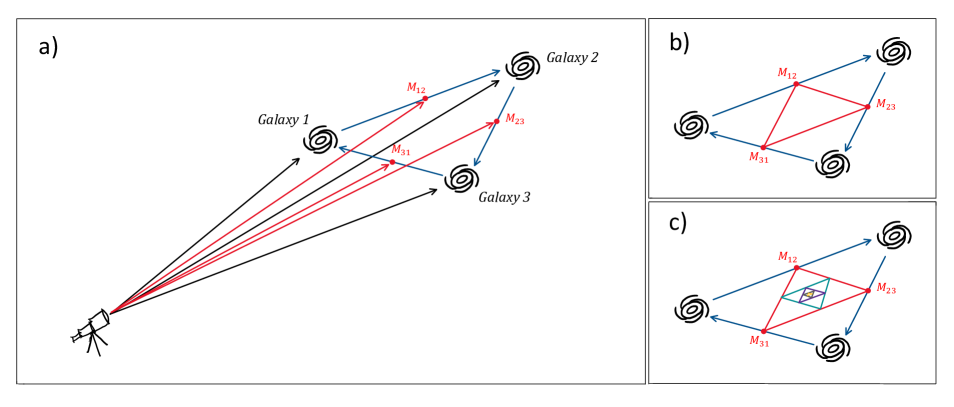
Figure 3: Illustration of the proof that a line of sight taken as the sum of the three galaxy position vectors, as in equation (8), will intersect the centroid of the base triangle formed by the three galaxies. In panel (a) we are summing each pair of positions as $\vec{x}_{i}+\vec{x}_{j}$, and the vector given by half this sum intersects the base triangle at the points indicated in red and labeled $M_{ij}$. These points are in fact the midpoints of the three base triangle sides, due to the fact that each sum $\vec{x}_{i}+\vec{x}_{j}$ could be represented by a parallelogram (as shown in Figure 2), whose diagonals always bisect each other. In panel (b) we connect these three intersection points, to form a triangle within the base triangle. It turns out that, since the $M_{ij}$ are midpoints, this $inner$ triangle is known as the medial triangle. The medial triangle of a given parent triangle will always share the same centroid. In panel (c) we repeat the process shown in (a) and (b) but now starting with the medial triangle as our new mother triangle. Panel (c) shows a number of iterations of this process. We can develop smaller and smaller concentric medial triangles by forming more and more sums of pairwise sums of the original vectors $\vec{x}_{i}$ and $\vec{x}_{j}$. These sums will all be rescalings of our desired line of sight, and hence pass through the base at the same point. Ultimately this point will be the only point remaining enclosed as we go to arbitrarily small medial triangles, meaning that our line of sight must pass through the centroid.

4.2 Centroid vs. Unit-Vector-Average Methods

We now seek to determine at what order our two methods differ from each other. We compute find $\hat{n}_{C}-\hat{n}_{U}$, which is

$$\hat{n}_{C}-\hat{n}_{U} =\frac{\vec{n}_{\rm C}}{|\vec{n}_{\rm C}|}-\frac{\vec{n}_{\rm U}}{|\vec{n}_{\rm U}|}$$ (10)

$$=\frac{\vec{x}_{1}+\vec{x}_{2}+\vec{x}_{3}}{|\vec{x}_{1}+\vec{x}_{2}+\vec{x}_{3}|}-\frac{\hat{x}_{1}+\hat{x}_{2}+\hat{x}_{3}}{|\hat{x}_{1}+\hat{x}_{2}+\hat{x}_{3}|}.$$

We first examine $\hat{n}_{C}$. Substituting $\vec{x}_{2}=\vec{x}_{1}+\vec{r}_{12}$ and $\vec{x}_{3}=\vec{x}_{1}+\vec{r}_{13}$ based on equation (3), and simplifying, we find

$$\vec{n}_{\rm C} =3\vec{x}_{1}+\vec{r}_{12}+\vec{r}_{13}$$

$$=3x_{1}[\hat{x}_{1}+\vec{r}_{12}/(3x_{1})+\vec{r}_{13}/(3x_{1})].$$ (11)

Defining

$$\epsilon_{12,1}\equiv r_{12}/(3x_{1}),$$

$$\epsilon_{13,1}\equiv r_{13}/(3x_{1}),$$ (12)

we can turn equation (4.2) into

$$\vec{n}_{\rm C} =\hat{x}_{1}+\epsilon_{12,1}\hat{r}_{12}+\epsilon_{13,1}\hat{r}_{13}.$$ (13)

Since we want $\hat{n}_{C}=\vec{n}_{\rm C}/|\vec{n}_{\rm C}|$, we will need to expand the denominator of this equation:

$$|\vec{n_{C}}|^{-1} =(|\hat{x}_{1}+\epsilon_{12,1}\hat{r}_{12}+\epsilon_{13,1}\hat{r}_{13}|^{2})^{-1/2}$$ (14)

$$=[1+2\hat{x}_{1}\cdot(\epsilon_{12,1}\hat{r}_{12}+\epsilon_{13,1}\hat{r}_{13})+\mathcal{O}(\epsilon^{2})]^{-1/2}$$

$$\approx 1-\epsilon_{12,1}\hat{r}_{12}\cdot\hat{x}_{1}-\epsilon_{13,1}\hat{r}_{13}\cdot\hat{x}_{1},$$

to finally obtain

$$\hat{n}_{C}=(\hat{x}_{1}+\epsilon_{12,1}\hat{r}_{12}+\epsilon_{13,1}\hat{r}_{13})(1-\epsilon_{12,1}\hat{r}_{12}\cdot\hat{x}_{1}-\epsilon_{13,1}\hat{r}_{13}\cdot\hat{x}_{1})$$

$$=\hat{x}_{1}+\epsilon_{12,1}[\hat{r}_{12}-(\hat{r}_{12}\cdot\hat{x}_{1})\hat{x}_{1}]+\epsilon_{13,1}[\hat{r}_{13}-(\hat{r}_{13}\cdot\hat{x}_{1})\hat{x}_{1}].$$ (15)

We now examine $\hat{n}_{U}$. We can rewrite the direction vector to the galaxy at $\vec{x}_{2}$ as

$$\hat{x}_{2} =\frac{\vec{x}_{1}+\vec{r}_{12}}{|\vec{x}_{1}+\vec{r}_{12}|}=\frac{\hat{x}_{1}+3\epsilon_{12,1}\hat{r}_{12}}{|\hat{x}_{1}+3\epsilon_{12,1}\hat{r}_{12}|},$$ (16)

and at $\vec{x}_{3}$ as

$$\hat{x}_{3} =\frac{\vec{x}_{1}+\vec{r}_{13}}{|\vec{x}_{1}+\vec{r}_{13}|}=\frac{\hat{x}_{1}+3\epsilon_{13,1}\hat{r}_{13}}{|\hat{x}_{1}+3\epsilon_{13,1}\hat{r}_{13}|}.$$ (17)

Thus $\vec{n}_{\rm U}$ will be

$$\vec{n}_{\rm U} =\hat{x}_{1}+\frac{\hat{x}_{1}+3\epsilon_{12,1}\hat{r}_{12}}{|\hat{x}_{1}+3\epsilon_{12,1}\hat{r}_{12}|}+\frac{\hat{x}_{1}+3\epsilon_{13,1}\hat{r}_{13}}{|\hat{x}_{1}+3\epsilon_{13,1}\hat{r}_{13}|}.$$ (18)

Expanding $|\hat{x}_{1}+3\epsilon_{21,2}\hat{r}_{12}|^{-1}$, we find

$$|\hat{x}_{1}+3\epsilon_{21,2}\hat{r}_{12}|^{-1} =[(\hat{x}_{1}+3\epsilon_{12,1}\hat{r}_{12})^{2}]^{-1/2}$$

$$=[1+6\epsilon_{12,1}\hat{r}_{12}\cdot\hat{x}_{1}+(3\epsilon_{12,1})^{2}]^{-1/2}$$

$$\approx 1-3\epsilon_{12,1}\hat{r}_{12}\cdot\hat{x}_{1}+\mathcal{O}\left(\epsilon_{12,1}^{2}\right),$$ (19)

which leads to

$$\vec{n}_{\rm U} =\hat{x}_{1}+(\hat{x}_{1}+3\epsilon_{12,1}\hat{r}_{12})(1-3\epsilon_{12,1}\hat{r}_{12}\cdot\hat{x}_{1})$$

$$+(\hat{x}_{1}+3\epsilon_{13,1}\hat{r}_{13})(1-3\epsilon_{13,1}\hat{r}_{13}\cdot\hat{x}_{1})$$

$$=3\{\hat{x}_{1}+\epsilon_{12,1}[\hat{r}_{12}-\hat{x}_{1}(\hat{r}_{12}\cdot\hat{x}_{1})]$$

$$+\epsilon_{13,1}[\hat{r}_{13}-\hat{x}_{1}(\hat{r}_{13}\cdot\hat{x}_{1})]\}$$ (20)

In order to find $\hat{n}_{U}=\vec{n}_{\rm U}/|\vec{n}_{\rm U}|$, we also need to expand the denominator of this equation as in

$$|\vec{n}_{\rm U}|^{-1} =\frac{1}{3}\bigg{\{}\bigg{[}\hat{x}_{1}+\epsilon_{12,1}[\hat{r}_{12}-\hat{x}_{1}(\hat{r}_{12}\cdot\hat{x}_{1})]$$

$$+\epsilon_{13,1}[\hat{r}_{13}-\hat{x}_{1}(\hat{r}_{13}\cdot\hat{x}_{1})]\bigg{]}^{2}\bigg{\}}^{-1/2}$$ (21)

$$=\frac{1}{3}\{1+\frac{2}{3}[3\epsilon_{12,1}(\hat{r}_{12}\cdot\hat{x}_{1}-\hat{r}_{12}\cdot\hat{x}_{1})(\hat{x}_{1}$$

$$-\epsilon_{12,1}[\hat{r}_{12}-\hat{x}_{1}(\hat{r}_{12}\cdot\hat{x}_{1})]-\epsilon_{13,1}[\hat{r}_{13}-\hat{x}_{1}(\hat{r}_{13}\cdot\hat{x}_{1})])^{2}]\}.$$

This has the form $\hat{x}_{1}^{2}+2\hat{x}_{1}\cdot\vec{v}+\vec{v}^{2}$, where $\vec{v}$ is here just a general vector. At $\mathcal{O}(\epsilon)$, we have $|\vec{n}_{\rm U}|^{-1}=1$. So up to (inclusive) $\mathcal{O}(\epsilon)$, we will have

$$\hat{n}_{U}\approx\hat{x}_{1} +\epsilon_{12,1}[\hat{r}_{12}-\hat{x}_{1}(\hat{r}_{12}\cdot\hat{x}_{1})]$$ (22)

$$+\epsilon_{13,1}[\hat{r}_{13}-\hat{x}_{1}(\hat{r}_{13}\cdot\hat{x}_{1})],$$

which is exactly what we found for $\hat{n}_{C}$. This means that

$$\hat{n}_{C}-\hat{n}_{U}=0$$ (23)

up to order $\mathcal{O}(\epsilon^{2})$.

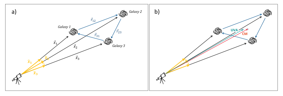
Figure 4: Representation of the unit vectors $\hat{x}_{1}$, $\hat{x}_{2}$, and $\hat{x}_{3}$ (yellow) in panel (a), and a comparison between the Centroid Method (CM) line-of-sight (which crosses the centroid of the triangle formed by the three galaxies; in teal), and the Unit-Vector-Average (UVA) method (scarlet) in panel (b).

5 Factorization of our basis

To extract the coefficient $\hat{\zeta}_{\ell_{1}\ell_{2}L}(r_{12},r_{13};\vec{x})$ we may use orthogonality:

$$\zeta_{\ell\ell_{2}\ell_{3}}(r_{12},r_{23})=\frac{1}{V}\int n^{2}dn\int d\Omega_{n}\;Y_{\ell}^{0*}(\hat{n})$$ (24)

$$\times\int d\Omega_{12}\;d\Omega_{13}\;Y^{m_{2}*}_{\ell_{2}}(\hat{r}_{12})Y^{m_{3}*}_{\ell_{3}}(\hat{r}_{13})\;\delta(\vec{x}_{1})\delta(\vec{x}_{1}+\vec{r}_{12})\delta(\vec{x}_{1}+\vec{r}_{13}).$$

where we now understand $\vec{x}_{1}$ to be a function of $\vec{n}$ and $\vec{r}_{12}$ and $\vec{r}_{13}$.

However , actually evaluating the above seems to require a triplet count: we have to look at the triplet of points $\vec{x}_{1}$, $\vec{x}_{1}+\vec{r}_{12}$, and $\vec{x}_{1}+\vec{r}_{13}$ to construct $\hat{n}$ if we set $\hat{n}=\hat{n}_{\rm C}$ or $\hat{n}_{\rm U}$.

We ask if $\vec{n}$ can be rewritten as a function of $\vec{x}_{1},\vec{r}_{12}$ and $\vec{r}_{13}$. We then ask if the spherical harmonic of $\hat{n}$ can be factorized into a product of functions of these, so that the integrand factorizes. If these were possible, we could then rewrite the integration as one over $d^{3}\vec{x}_{1}\;d\Omega_{12}\;d\Omega_{13}$ and compute each integration separately. We could sit at a point $\vec{x}_{1}$ perform the inner two integrals independently from each other, and hence obtain an algorithm scaling as $N^{2}$ much in the same way that Slepian & Eisenstein (2015d) does. Hence, we rewrite the triple product of spherical harmonics on the righthand side above in terms of $\hat{x}_{1}$, $\hat{r}_{12}$, and $\hat{r}_{13}$. This may be done using the results in our Appendix LABEL:app:app1, of which we duplicate the key equations here.

$$Y_{\ell}^{m} (\savestack{\tmpbox}{\stretchto{\scaleto{\scalerel*[\widthof{3\vec{x}_{1}+\vec{r}_{12}+\vec{r}_{13}}]{\kern-0.6pt\bigwedge\kern-0.6pt}{\rule[-505.89pt]{4.30554pt}{505.89pt}}}{}}{0.5ex}}\stackon[1pt]{3\vec{x}_{1}+\vec{r}_{12}+\vec{r}_{13}}{\tmpbox})=4\pi\sum_{n=0}^{\infty}\sum_{k=0}^{\lfloor n/2\rfloor}\;\sum_{z=0}^{n-2k}\;\sum_{z^{\prime}=0}^{k}\;\sum_{z^{\prime\prime}=0}^{k-z^{\prime}}\;\sum$$

$$\times\sum_{m=-j}^{j}\;\sum_{j^{\prime}=(n-2k-z)\downarrow 2}\;\sum_{m^{\prime}=-j^{\prime}}^{j^{\prime}}\;\sum_{j^{\prime\prime}=z\downarrow 2}\;\sum_{m^{\prime\prime}=-j^{\prime\prime}}^{j^{\prime\prime}}\;\sum_{\lambda=0}^{\ell}\;\sum_{\lambda^{\prime}=0}^{\ell-\lambda}$$

$$\times\sum_{\mu=-\lambda}^{\lambda}\;\sum_{\mu^{\prime}=-\lambda^{\prime}}^{\lambda^{\prime}}\;\sum_{L_{0}M_{0}}\;\sum_{\mathcal{L}_{0}\mathcal{M}_{0}}\;\sum_{L_{1}M_{1}}\;\sum_{\mathcal{L}_{1}\mathcal{M}_{1}}\;\sum_{L_{2}M_{2}}\;\sum_{\mathcal{L}_{2}\mathcal{M}_{2}}$$

$$\times\mathcal{U}_{zz^{\prime}z^{\prime\prime}jj^{\prime}j^{\prime\prime}}^{kn\;(\ell/2)}\;Q_{\ell\lambda\lambda^{\prime}}\;\mathcal{G}_{\lambda\lambda^{\prime}jj^{\prime}j^{\prime\prime}L_{0}\mathcal{L}_{0}L_{1}\mathcal{L}_{1}\ell L_{2}\mathcal{L}_{2}}^{\mu\mu^{\prime}mm^{\prime}m^{\prime\prime}M_{0}\mathcal{M}_{0}M_{1}\mathcal{M}_{1}M_{2}\mathcal{M}_{2}}$$

$$\times\epsilon_{12,1}^{n-z-z^{\prime}-2z^{\prime\prime}+\lambda^{\prime}}\;\epsilon_{13,1}^{z+z^{\prime}+2z^{\prime\prime}+\ell-\lambda-\lambda^{\prime}}$$ (25)

$$\times Y_{L_{0}}^{M_{0}}(\hat{x}_{1})\;Y_{L_{1}}^{M_{1}}(\hat{r}_{12})\;Y_{L_{2}}^{M_{2}}(\hat{r}_{13}),$$

where

$$\mathcal{U}_{zz^{\prime}z^{\prime\prime}jj^{\prime}j^{\prime\prime}}^{kn\alpha}\equiv\frac{4\pi^{2}}{(2j^{\prime}+1)(2j^{\prime\prime}+1)}\;\mathcal{T}_{zz^{\prime}z^{\prime\prime}}^{jkn\alpha}\;\mathcal{S}_{j^{\prime}}^{n-2k-z}\;\mathcal{S}_{j^{\prime\prime}}^{z},$$ (26)

$$\mathcal{T}_{zz^{\prime}z^{\prime\prime}}^{jkn\alpha}\equiv\frac{\Gamma(n-k+\alpha)}{\Gamma(\alpha)}$$ (27)

$$\times\frac{4\pi\;(-1)^{k}\;(2)^{z^{\prime}+2n-4k-(z^{\prime}-j)/2}}{z!\;z^{\prime\prime}!\;(n-2k-z)!\;(k-z^{\prime}-z^{\prime\prime})!\;[(z^{\prime}-j)/2]!\;(j+z^{\prime}+1)!!}$$

$$\mathcal{S}_{j}^{z^{\prime}}\equiv\frac{(2j+1)z^{\prime}!}{2^{(z^{\prime}-j)/2}((z^{\prime}-j)/2)!(j+z^{\prime}+1)!!}.$$ (28)

$$\mathcal{Q}_{\ell\lambda\lambda^{\prime}} \equiv\begin{pmatrix}2\ell\\ 2\lambda\end{pmatrix}^{1/2}\begin{pmatrix}2(\ell-\lambda)\\ 2\lambda^{\prime}\end{pmatrix}^{1/2}(-1)^{\lambda+\mu}\sqrt{2\ell+1}\sqrt{2(\ell-\lambda)+1}$$

$$\times\begin{pmatrix}\lambda&\ell-\lambda&\ell\\ \mu&m-\mu&-m\end{pmatrix}\begin{pmatrix}\lambda^{\prime}&\ell-\lambda-\lambda^{\prime}&\ell-\lambda\\ \mu^{\prime}&m-\mu-\mu^{\prime}&-m+\mu\end{pmatrix},$$ (29)

and

$$\mathcal{G} {}_{\lambda\lambda^{\prime}jj^{\prime}j^{\prime\prime}L_{0}\mathcal{L}_{0}L_{1}\mathcal{L}_{1}\ell L_{2}\mathcal{L}_{2}}^{\mu\mu^{\prime}mm^{\prime}m^{\prime\prime}M_{0}\mathcal{M}_{0}M_{1}\mathcal{M}_{1}M_{2}\mathcal{M}_{2}}\equiv$$ (30)

$$\hskip 56.9055pt\mathcal{G}_{\lambda j^{\prime}\mathcal{L}_{0}}^{\mu-m^{\prime}-\mathcal{M}_{0}}\;\mathcal{G}_{\mathcal{L}_{0}j^{\prime\prime}L_{0}}^{\mathcal{M}_{0}-m^{\prime\prime}-M_{0}}\;\mathcal{G}_{\lambda^{\prime}j\mathcal{L}_{1}}^{\mu^{\prime}m-\mathcal{M}_{1}}$$

$$\hskip 56.9055pt\times\mathcal{G}_{\mathcal{L}_{1}j^{\prime}L_{1}}^{\mathcal{M}_{1}m^{\prime}-M_{1}}\;\mathcal{G}_{(\ell-\lambda-\lambda^{\prime})j\mathcal{L}_{2}}^{(m-\mu-\mu^{\prime})-m-\mathcal{M}_{2}}\;\mathcal{G}_{\mathcal{L}_{2}j^{\prime\prime}L_{2}}^{\mathcal{M}_{2}m^{\prime\prime}-M_{2}}.$$

The summation indices of equation (5), their limits, and detailed explanation can be found in Table LABEL:table1. We present here only the result for the Centroid method because the Unit-Vector-Average method agrees with it at $\mathcal{O}(\theta^{2})$, as shown in §4. However if one wished to go beyond that order, applying the math in Appendix LABEL:app:app1 to do so is straightforward.

6 Leading-Order Correction from Our Approach

Since $\epsilon_{12,1}$ and $\epsilon_{13,1}$ are of the same order, we can suppose that they represent the same variable and analyze the sum of their powers to find the leading-order correction required by our approach, i.e. to find all terms that lead to a contribution at $\mathcal{O}(\epsilon)$. Taking it that $\epsilon_{12,1}\simeq\epsilon_{13,1}\simeq\epsilon$, we see that equation (5) behaves as

$$\epsilon^{n-z-z^{\prime}-2z^{\prime\prime}+\lambda^{\prime}}\epsilon^{z+z^{\prime}+2z^{\prime\prime}+\ell-\lambda-\lambda^{\prime}}\simeq\epsilon^{n+\ell-\lambda}.$$ (31)

We see that at $\mathcal{O}(\epsilon)$, there are two possible cases that can contribute. We must have $n+\ell-\lambda=1$. The first way this can happen is when $n=0$ and $\ell-\lambda=1$. In this first case we reduce equation (5) to

For $\ell=0$ and $m=0$:

$$R_{0}^{0}(\vec{r}+\vec{s})=\frac{1}{2}\left[R_{0}^{0}(\vec{r})+R_{0}^{0}(\vec{s})\right]=1.$$ (97)

For $\ell=1$ and $m=0$:

$$R_{1}^{0}(\vec{r}+\vec{s})=r_{z}+s_{z}.$$ (98)

For $\ell=1$ and $m=1$:

$$R_{1}^{1}(\vec{r}+\vec{s}) =-\frac{\sqrt{2}}{2}[r_{x}+s_{x}+i(r_{y}+s_{y})]$$ (99)

$$=-\frac{\sqrt{2}}{2}(r_{x}+ir_{y})-\frac{\sqrt{2}}{2}(s_{x}+is_{y})$$

Here, $-(\sqrt{2}/2)(r_{x}+ir_{y})$ and $-(\sqrt{2}/2)(s_{x}+is_{y})$ are $R_{1}^{1}(\vec{r})$ and $R_{1}^{1}(\vec{s})$ (see Table LABEL:table2), respectively. So we find

$$R_{1}^{1}(\vec{r}+\vec{s}) =R_{1}^{1}(\vec{r})+R_{1}^{1}(\vec{s}).$$ (100)

For $\ell=1$ and $m=-1$:

Following the same logic, for $\ell=1$ and $m=-1$ we find that

$$R_{1}^{-1}(\vec{r}+\vec{s}) =R_{1}^{-1}(\vec{r})+R_{1}^{-1}(\vec{s}).$$ (101)

For $\ell=2$ and $m=0$:

$$R_{2}^{0}(\vec{r}+\vec{s})=-\frac{1}{2}[2(r_{z}+s_{z})^{2}-(r_{x}+s_{x})^{2}-(r_{y}+s_{y})^{2}]$$ (102)

which we find after expanding each term

$$R_{2}^{0}(\vec{r}+\vec{s}) =R_{2}^{0}(\vec{r})+R_{2}^{0}(\vec{s})+2r_{z}s_{z}-r_{x}s_{x}-r_{y}s_{y}$$ (103)

$$=R_{2}^{0}(\vec{r})+R_{2}^{0}(\vec{s})+2R_{1}^{0}(\vec{r})R_{1}^{0}(\vec{s})-r_{x}s_{x}-r_{y}s_{y}$$

We know from the derivation of $R_{1}^{1}(\vec{v})$ and $R_{1}^{-1}(\vec{v})$ above that

$$v_{x} =\frac{1}{\sqrt{2}}[R_{1}^{-1}(\vec{v})-R_{1}^{1}(\vec{v})]$$ (104)

$$v_{y} =-\frac{1}{i\sqrt{2}}[R_{1}^{1}(\vec{v})+R_{1}^{-1}(\vec{v})]$$ (105)

After substituting these into Eq. (103), we find that

$$R_{2}^{0}(\vec{r}+\vec{s}) =R_{2}^{0}(\vec{r})+R_{2}^{0}(\vec{s})+2R_{1}^{0}(\vec{r})R_{1}^{0}(\vec{s})$$

$$-\frac{1}{2}\big{[}R_{1}^{-1}(\vec{r})R_{1}^{-1}(\vec{s})+R_{1}^{-1}(\vec{r})R_{1}^{1}(\vec{s})$$

$$+R_{1}^{1}(\vec{r})R_{1}^{-1}(\vec{s})+R_{1}^{1}(\vec{r})R_{1}^{1}(\vec{s})\big{]}$$ (106)

$$-\frac{1}{2}\big{[}R_{1}^{1}(\vec{r})R_{1}^{1}(\vec{s})+R_{1}^{1}(\vec{r})R_{1}^{-1}(\vec{s})$$

$$+R_{1}^{-1}(\vec{r})R_{1}^{1}(\vec{s})+R_{1}^{-1}(\vec{r})R_{1}^{-1}(\vec{s})\big{]},$$

which simplifying becomes

$$R_{2}^{0}(\vec{r}+\vec{s}) =R_{2}^{0}(\vec{r})+R_{2}^{0}(\vec{s})+2R_{1}^{0}(\vec{r})R_{1}^{0}(\vec{s})$$ (107)

$$+R_{1}^{1}(\vec{r})R_{1}^{-1}(\vec{s})+R_{1}^{-1}(\vec{r})R_{1}^{1}(\vec{s})$$

For $\ell=2$ and $m=1$:

$$R_{2}^{1}(\vec{r} +\vec{s})=-\frac{\sqrt{6}}{2}\left[r_{x}+s_{x}+i(r_{y}+s_{y})\right](r_{z}+s_{z})$$

$$=-\frac{\sqrt{6}}{2}(r_{x}+ir_{y})r_{z}-\frac{\sqrt{6}}{2}(s_{x}+is_{y})s_{z}$$ (108)

$$\hskip 8.53581pt-\frac{\sqrt{6}}{2}(r_{x}+ir_{y})s_{z}-\frac{\sqrt{6}}{2}(s_{x}+is_{y})r_{z}$$

$$=R_{2}^{1}(\vec{r})+R_{2}^{1}(\vec{s})+\sqrt{3}\left[R_{1}^{1}(\vec{r})R_{1}^{0}(\vec{s})+R_{1}^{1}(\vec{s})R_{1}^{0}(\vec{r})\right]$$

For $\ell=2$ and $m=-1$:

$$R_{2}^{1}(\vec{r} +\vec{s})=\frac{\sqrt{6}}{2}\left[r_{x}+s_{x}-i(r_{y}+s_{y})\right](r_{z}+s_{z})$$

$$=\frac{\sqrt{6}}{2}(r_{x}-ir_{y})r_{z}+\frac{\sqrt{6}}{2}(s_{x}-is_{y})s_{z}$$ (109)

$$\hskip 8.53581pt\frac{\sqrt{6}}{2}(r_{x}-ir_{y})s_{z}+\frac{\sqrt{6}}{2}(s_{x}-is_{y})r_{z}$$

$$=R_{2}^{-1}(\vec{r})+R_{2}^{-1}(\vec{s})+\sqrt{3}\left[R_{1}^{-1}(\vec{r})R_{1}^{0}(\vec{s})+R_{1}^{-1}(\vec{s})R_{1}^{0}(\vec{r})\right]$$

For $\ell=2$ and $m=2$:

$$R_{2}^{2}(\vec{r} +\vec{s})=\frac{\sqrt{6}}{4}(r_{x}+ir_{y}+s_{x}+is_{y})^{2}$$ (110)

$$=\frac{\sqrt{6}}{4}\left[(r_{x}+ir_{y})^{2}+2(r_{x}+ir_{y})(s_{x}+is_{y})+(s_{x}+is_{y})^{2}\right]$$

$$=R_{2}^{2}(\vec{r})+R_{2}^{2}(\vec{s})+\sqrt{6}R_{1}^{1}(\vec{r})R_{1}^{1}(\vec{s})$$

For $\ell=2$ and $m=-2$:

$$R_{2}^{2}(\vec{r} +\vec{s})=\frac{\sqrt{6}}{4}(r_{x}-ir_{y}+s_{x}-is_{y})^{2}$$ (111)

$$=\frac{\sqrt{6}}{4}\left[(r_{x}-ir_{y})^{2}+2(r_{x}-ir_{y})(s_{x}-is_{y})+(s_{x}-is_{y})^{2}\right]$$

$$=R_{2}^{-2}(\vec{r})+R_{2}^{-2}(\vec{s})+\sqrt{6}R_{1}^{-1}(\vec{r})R_{1}^{-1}(\vec{s})$$

Table 2: Spherical and solid harmonics of $\hat{r}$ and $\vec{r}$, respectively, for $\ell=\{0,1,2\}$.

Solid Harmonics
$\ell$	$m$	$Y_{\ell}^{m}(\hat{r})$	$R_{\ell}^{m}(\vec{r})=\sqrt{\frac{4\pi}{2\ell+1}}r^{\ell}Y_{\ell}^{m}(\hat{r})$
0	0	$\frac{1}{2}\sqrt{\frac{1}{\pi}}$	1
1	-1	$\frac{1}{2}\sqrt{\frac{3}{2\pi}}(r_{x}-ir_{y})\;r^{-1}$	$\frac{\sqrt{2}}{2}(r_{x}-ir_{y})$
1	0	$\frac{1}{2}\sqrt{\frac{3}{\pi}}r_{z}\;r^{-1}$	$r_{z}$
1	1	$-\frac{1}{2}\sqrt{\frac{3}{2\pi}}(r_{x}+ir_{y})\;r^{-1}$	$-\frac{\sqrt{2}}{2}(r_{x}+ir_{y})$
2	-2	$\frac{1}{4}\sqrt{\frac{15}{2\pi}}(r_{x}-ir_{y})^{2}\;r^{-2}$	$\frac{\sqrt{6}}{4}(r_{x}-ir_{y})^{2}$
2	-1	$\frac{1}{2}\sqrt{\frac{15}{2\pi}}(r_{x}-ir_{y})\;z\;r^{-2}$	$\frac{\sqrt{6}}{2}(r_{x}-ir_{y})\;r_{z}$
2	0	$\frac{1}{4}\sqrt{\frac{5}{\pi}}(2r_{z}^{2}-r_{x}^{2}-r_{y}^{2})\;r^{-2}$	$\frac{1}{2}(2r_{z}^{2}-r_{x}^{2}-r_{y}^{2})$
2	1	$-\frac{1}{2}\sqrt{\frac{15}{2\pi}}(r_{x}+ir_{y})\;z\;r^{-2}$	$-\frac{\sqrt{6}}{2}(r_{x}+ir_{y})\;r_{z}$
2	2	$\frac{1}{4}\sqrt{\frac{15}{2\pi}}(r_{x}+ir_{y})^{2}\;r^{-2}$	$\frac{\sqrt{6}}{4}(r_{x}+ir_{y})^{2}$

Appendix C Product to Sum Expansions for Spherical Harmonics

Here we show how a product of three spherical harmonics of the same argument can be turned into a sum over single harmonics. We start with the product of two spherical harmonics ($Y_{l_{1}}^{m_{1}}(\hat{x})$ and $Y_{l_{2}}^{m_{2}}(\hat{x})$), which can be written as a sum of other spherical harmonics times a coefficient $C_{l_{1}l_{2}L}^{m_{1}m_{2}M}$ as in

$$Y_{l_{1}}^{m_{1}}(\hat{x})\;Y_{l_{2}}^{m_{2}}(\hat{x})=\sum_{LM}C_{l_{1}l_{2}L}^{m_{1}m_{2}M}\;Y_{L}^{M}(\hat{x}).$$ (124)

Multiplying both sides by $\int d\Omega_{x}Y_{L}^{M*}(\hat{x})$ we obtain:

$$\int d\Omega_{x}Y_{l_{1}}^{m_{1}}(\hat{x})\;Y_{l_{2}}^{m_{2}}(\hat{x})\;Y_{L}^{M*}(\hat{x})=C_{l_{1}l_{2}L}^{m_{1}m_{2}M}.$$ (125)

We know that

$$Y_{L}^{M*}(\hat{x})=(-1)^{M}Y_{L}^{-M}(\hat{x}).$$ (126)

Thus we find

$$(-1)^{M}\int d\Omega_{x}Y_{l_{1}}^{m_{1}}(\hat{x})\;Y_{l_{2}}^{m_{2}}(\hat{x})\;Y_{L}^{-M}(\hat{x})=C_{l_{1}l_{2}L}^{m_{1}m_{2}M}$$ (127)

The integral above is the Gaunt integral, which we denote

$$\mathcal{G}_{l_{1}l_{2}L}^{m_{1}m_{2}-M}= \sqrt{\frac{(2l_{1}+1)(2l_{2}+2)(2l_{3}+3)}{4\pi}}$$

$$\times\begin{pmatrix}l_{1}&l_{2}&L\\ 0&0&0\end{pmatrix}\begin{pmatrix}l_{1}&l_{2}&L\\ m_{1}&m_{2}&-M\end{pmatrix}.$$ (128)

Substituting equation (C) into equation (127) we obtain

$$C_{l_{1}l_{2}L}^{m_{1}m_{2}M}=(-1)^{M}\mathcal{G}_{l_{1}l_{2}L}^{m_{1}m_{2}-M}.$$ (129)

Now we want to extend this result to the product of three spherical harmonics, i.e.

$$Y_{l_{1}}^{m_{1}}(\hat{x})Y_{l_{2}}^{m_{2}}(\hat{x})Y_{l_{3}}^{m_{3}}(\hat{x})=\sum_{LM}D_{l_{1}l_{2}l_{3}L}^{m_{1}m_{2}m_{3}M}\;Y_{L}^{M}(\hat{x}).$$ (130)

Multiplying both sides of equation (130) by $\int d\Omega_{x}Y_{L}^{M*}(\hat{x})$ we find:

$$\int d\Omega_{x}Y_{l_{1}}^{m_{1}}(\hat{x})\;Y_{l_{2}}^{m_{2}}(\hat{x})\;Y_{l_{3}}^{m_{3}}(\hat{x})\;Y_{L}^{M*}(\hat{x})=D_{l_{1}l_{2}l_{3}L}^{m_{1}m_{2}m_{3}M}$$ (131)

Transforming the conjugate using $Y_{L}^{M*}(x)=(-1)^{M}Y_{L}^{-M}(x)$ we obtain:

$$(-1)^{M}\int d\Omega_{x}Y_{l_{1}}^{m_{1}}(\hat{x})\;Y_{l_{2}}^{m_{2}}(\hat{x})\;Y_{l_{3}}^{m_{3}}(\hat{x})\;Y_{L}^{-M}(\hat{x})=D_{l_{1}l_{2}l_{3}L}^{m_{1}m_{2}m_{3}M}$$ (132)

From equation (124) we see that

$$Y_{l_{1}}^{m_{1}}(\hat{x})\;Y_{l_{2}}^{m_{2}}(\hat{x})=\sum_{\mathcal{L}\mathcal{M}}C_{l_{1}l_{2}\mathcal{L}}^{m_{1}m_{2}\mathcal{M}}\;Y_{\mathcal{L}}^{\mathcal{M}}(\hat{x})$$ (133)

Thus, if we substitute equation (133) in equation (132) we obtain

$$\int d\Omega_{x}\;\sum_{\mathcal{L}\mathcal{M}} (-1)^{M+\mathcal{M}}\;C_{l_{1}l_{2}\mathcal{L}}^{m_{1}m_{2}\mathcal{M}}$$ (134)

$$\times Y_{\mathcal{L}}^{\mathcal{M}}(\hat{x})\;Y_{l_{3}}^{m_{3}}(\hat{x})\;Y_{L}^{-M}(\hat{x})=D_{l_{1}l_{2}l_{3}L}^{m_{1}m_{2}m_{3}M},$$

which based on equation (C) we know is

$$\sum_{\mathcal{L}\mathcal{M}}(-1)^{M+\mathcal{M}}\;C_{l_{1}l_{2}\mathcal{L}}^{m_{1}m_{2}\mathcal{M}}\;\mathcal{G}_{\mathcal{L}l_{3}L}^{\mathcal{M}m_{3}-M}=D_{l_{1}l_{2}l_{3}L}^{m_{1}m_{2}m_{3}M}.$$ (135)

And by substituting equation (129) in equation (135) we find

$$D_{l_{1}l_{2}l_{3}L}^{m_{1}m_{2}m_{3}M}=\sum_{\mathcal{L}\mathcal{M}}(-1)^{M+\mathcal{M}}\;\mathcal{G}_{l_{1}l_{2}\mathcal{L}}^{m_{1}m_{2}-\mathcal{M}}\;\mathcal{G}_{\mathcal{L}l_{3}L}^{\mathcal{M}m_{3}-M}.$$ (136)

Finally, substituting equation (136) in equation (130) we obtain

$$Y_{l_{1}}^{m_{1}}(\hat{x})Y_{l_{2}}^{m_{2}} (\hat{x})Y_{l_{3}}^{m_{3}}(\hat{x})=$$ (137)

$$\sum_{LM}\sum_{\mathcal{L}\mathcal{M}}(-1)^{M+\mathcal{M}}\mathcal{G}_{l_{1}l_{2}\mathcal{L}}^{m_{1}m_{2}-\mathcal{M}}\;\mathcal{G}_{\mathcal{L}l_{3}L}^{\mathcal{M}m_{3}-M}\;Y_{L}^{M}(\hat{x}).$$

References

- Bernardeau et al. (2002) Bernardeau F., Colombi S., Gaztañaga E., Scoccimarro R., 2002, Phys. Rep., 367, 1
- Cahn & Slepian (2020) Cahn R. N., Slepian Z., 2020, Isotropic N-Point Basis Functions and Their Properties (arXiv:2010.14418)
- Chan et al. (2012) Chan K. C., Scoccimarro R., Sheth R. K., 2012, Physical Review D, 85
- Desjacques et al. (2018) Desjacques V., Jeong D., Schmidt F., 2018, Phys. Rep., 733, 1
- Friesen et al. (2017) Friesen B., et al., 2017, Proceedings of the International Conference for High Performance Computing, Networking, Storage and Analysis
- Fry & Gaztanaga (1993) Fry J. N., Gaztanaga E., 1993, ApJ, 413, 447
- Gagrani & Samushia (2017) Gagrani P., Samushia L., 2017, MNRAS, 467, 928
- Gaztanaga (1994) Gaztanaga E., 1994, MNRAS, 268, 913
- Gil-Marín et al. (2015) Gil-Marín H., Noreña J., Verde L., Percival W. J., Wagner C., Manera M., Schneider D. P., 2015, Monthly Notices of the Royal Astronomical Society, 451, 539–580
- Gualdi & Verde (2020) Gualdi D., Verde L., 2020, Journal of Cosmology and Astroparticle Physics, 2020, 041–041
- Guo et al. (2015) Guo H., et al., 2015, Monthly Notices of the Royal Astronomical Society: Letters, 449, L95–L99
- Jackson (1972) Jackson J. C., 1972, MNRAS, 156, 1P
- Jing & Borner (2004) Jing Y. P., Borner G., 2004, The Astrophysical Journal, 607, 140–163
- Kaiser (1987) Kaiser N., 1987, MNRAS, 227, 1
- Levi et al. (2019) Levi M. E., et al., 2019, The Dark Energy Spectroscopic Instrument (DESI) (arXiv:1907.10688)
- McDonald & Roy (2009) McDonald P., Roy A., 2009, Journal of Cosmology and Astro-Particle Physics, 2009, 020
- Pearson & Samushia (2018) Pearson D. W., Samushia L., 2018, MNRAS, 478, 4500
- Rampf & Wong (2012) Rampf C., Wong Y. Y., 2012, Journal of Cosmology and Astroparticle Physics, 2012, 018–018
- Schlegel et al. (2019) Schlegel D. J., et al., 2019, Astro2020 APC White Paper: The MegaMapper: a z > 2 spectroscopic instrument for the study of Inflation and Dark Energy (arXiv:1907.11171)
- Scoccimarro (2015) Scoccimarro R., 2015, Physical Review D, 92
- Scoccimarro et al. (1999) Scoccimarro R., Couchman H. M. P., Frieman J. A., 1999, The Astrophysical Journal, 517, 531–540