Bondi-Hoyle Accretion around the Non-rotating Black Hole in 4D Einstein-Gauss-Bonnet Gravity

Abstract

In this paper, the numerical investigation of a Bondi-Hoyle accretion around a non-rotating black hole in a novel four dimensional Einstein-Gauss-Bonnet gravity is investigated by solving the general relativistic hydrodynamical equations using the high resolution shock capturing scheme. For this purpose, the accreated matter from the wind-accreating $X-$ray binaries falls towards the black hole from the far upstream side of the domain, suphersonically. We study the effects of Gauss-Bonnet coupling constant $\alpha$ in $4D$ EGB gravity on the accreated matter and shock cones created in the downstream region in detail. The required time having the shock cone in downstream region is getting smaller for $\alpha>0$ while it is increasing for $\alpha<0$. It is found that increases in $\alpha$ leads violent oscillations inside the shock cone and increases the accretion efficiency. The violent oscillations would cause increase in the energy flux, temperature, and spectrum of $X-$ rays. So the quasi-periodic oscillations (QPOs) are naturally produced inside the shock cone when $-5\leq\alpha\leq 0.8$. It is also confirmed that EGB black hole solution converges to the Schwarzschild one in general relativity when $\alpha\rightarrow 0$. Besides, the negative coupling constants also give reasonable physical solutions and increase of $\alpha$ in negative directions suppresses the possible oscillation observed in the shock cone.

1 Introduction

Einstein’s general theory of relativity has successfully passed many observational tests during the last decades (Akiyama1 et. al., 2019; Akiyama2 et. al., 2019; Akiyama3 et. al., 2019; Abbott1 et. al., 2016; Abbott2 et. al., 2016). The existence of super-massive black hole at the center of galaxy M87 was one of the most impressive discoveries. The observed M87 black hole shadow indicates that the observed data well consistent with the prediction of the general theory of relativity. The observed gravitational waves created during the coalescing of two stellar mass black holes made by LIGO detectors was another discovery to see the ripples of the space time predicted by Einstein’s general theory of relativity. The observed electromagnetic spectrum emitted from an accretion disk around the black holes could allow us to define many properties of the black holes, such as mass, spin, etc.(Frank et. al., 2002; Yuan & Narayan, 2014; Nampalliwar & Bambi, 2019). All recent observations indicate that testing the general theory of relativity and its alternatives in a week and a strong gravitational regions are hot topics in this century. On this end, in order to extract more detailed information about the strong gravitational regimes around the black holes, we study the alternative theory to the Einstein’s theory of the relativity called four dimensional Einstein-Gauss-Bonnet (EGB) gravity which was first formulated by Glavan & Lin (2020).

A novel four-dimensional EGB gravity theory was proposed in Glavan & Lin (2020) where the Gauss-Bonnet coupling constant is $\alpha\rightarrow\alpha/(D-4)$ in the limit $D\rightarrow 4$ and bypasses the Lovelocks theorem. As a consequence of this limit, the Gauss-Bonnet coupling constant gives non-trivial contributions to the gravitational dynamics. It is also shown that the theory is free from Ostrogradsky instability and preserves the number of degrees of freedom. And the static spherically symmetric black hole, which has two horizons instead of one compared to the Schwarzschild black hole, was discovered(Cheng et. al., 2020). The horizon is rescaled with the Gauss-Bonnet coupling constant $\alpha$ and the causal structure of the black hole radically is altered with a repulsive effect. Although this $4D$ EGB theory is currently under debate (Julio et. al., 2020; Gurses et. al., 2020; Ai, 2020), it is worthy and meaningful to study the spherical symmetric black hole solution of $4D$ EGB gravity.

The newly discovered four-dimensional static and spherically symmetric Gauss-Bonnet black hole was used to reveal many interesting features of some astrophysical problems. Lots of work have been done the different astrophysical phenomena the viability of the solution. The properties of the black hole and its shadow (Konoplya & Zinhailo, 2020; Roy & Chakrabarti, 2020), the innermost stable circular orbit for massive particles and photons (Guo & Li, 2020; Zhang et. al., 2020), generating and radiating black hole (Ghosh & Maharaj, 2020; Ghosh & Kumar, 2020), week cosmic censorship conjecture (Yang et. al., 2020), the gravitational lensing by black holes (Jin et. al., 2020; Islam et. al., 2020), observational constraints on the Gauss-Bonnet constant (Feng et. al., 2020; Clifton et. al., 2020), the growth rate of non-relativistic matter perturbations (Zahra, 2020), and Greybody factor and power spectra of the Hawking radiation (Konoplya & Zinhailo, 2020; Zhang et. al., 2020) were studied with all details.

The wind accretion scenario onto the black hole is one of the important physical phenomena to explain soft and hard $X-$ rays observed by different $X-$ ray telescopes. The wind accretion process can be explained by using the Bondi-Hoyle model (Edgar, 2004). A black hole moving inside the gas cloud captures mass which causes either acceleration or deceleration of it. As a result of this the shock cone or bow shock would be formed around the black hole. This is the one of hot topics studied by different researchers using the analytical and the numerical techniques in the last few decades. Analytic representation of the wind accretion for a perfect fluid onto a Schwarzschild black hole has been found by Tejeda & Aguayo-Ortiz (2019) and numerical treatments from Newtonian and relativistic perspective were extensively studied by Donmez et. al. (2011); Donmez (2012); Cruz-Osorio & Lora-Clavijo (2016); Cruz-Osorio et. al. (2017).

In the present paper, building onto the previous findings, we would like to study the creation of the shock cones and their dynamical evolution in case of Bondi-Hoyle accretion in the background of the $4D$ EGB spherically symmetric black hole in the strong gravitational region, numerically. Bondi-Hoyle accretion is an important mechanism to explain Quasi-Periodic Oscillations (QPOs) observed by $X-ray$ telescope. The companion star in the $X-$ray binary system provide the fast wind which causes to accreate towards to the black hole(Orosz et. al., 2008). The accelerating single black holes due to the other black holes could have Bondi-Hoyle accretion(Lora et. al., 2013). Studying the QPOs on accretion disk in vicinity of a black hole is important to explore the physical parameters of the black hole such as its spin and mass. QPO arises in the inner accretion disk of the black hole binary and could be created in terms of an oscillating, precessing hot flow in the truncated-disk geometry due to the strong shocks. Therefore, it would be a further step to know whether the Gauss-Bonnet coupling constant $\alpha$ can play a dominant role in the oscillation of the shock cone created during the Bondi-Hoyle accretion. To reveal all these details, we numerically model the Bondi-Hoyle accretion in the vicinity of $4D$ EGB black hole. We compute the shock cone structures for different values of Gauss-Bonnet constant $\alpha$ and compare them with standard general relativistic solution, Schwarzschild black hole.

The plan of the paper is as follows: In Section 2, we briefly give summary of the recently proposed non-rotating black hole solution in $4D$ EGB gravity and definition of the horizon of the black hole. In section 3, we describe the conserved form of the general relativistic hydrodynamical equations, lapse function, and shift vectors in $4D$ EGB black hole necessary in our numerical simulations. In Section 4, we describe the theoretical framework of the Bondi-Hoyle accretion for pressureless gas, and initial and boundary conditions used in our numerical simulation. The numerical results and discussion are also given to show dependencies of the disk dynamics, creation of shock cones, accretion rates, and mode power to Gauss-Bonnet coupling constant $\alpha$. In Section 5, we discuss the implications from our numerical results and draw the direction of future work. Unless specified, we use geometrized units throughout the paper for the speed of light and gravitational constant, $G=c=1$.

2 Non-rotating Black Hole Solution of 4D EGB Gravity

The theory of the static and spherically symmetric solution of the gravity can be driven by summing Einstein-Hilbert action and higher order Lovelock invariants with the vanishing bare cosmological constant Glavan & Lin (2020).

$$S_{EH}+S_{GB}=\int{d^{D}x\sqrt{-g}\left(\frac{M^{2}_{P}}{2}R+\alpha G\right)},$$ (1)

where $M_{P}$, $R$, $\alpha$, and $G$ are the reduced Planck mass, the Ricci scalar of the space-time, the Gauss-Bonnet coupling constant, and the Gauss-Bonnet invariant, respectively (Glavan & Lin, 2020; Cheng et. al., 2020). The theory of this black hole was already established for $D\geq 5$ (Boulware & S. Deser, 2020). But the Gauss-Bonnet term $G$ does not contribute to the $4D$ gravitational dynamics. The reason is that the equation of a motion contains term $D-4$ and it will disappear while $D=4$. After rescaling the coupling constant $\alpha\rightarrow\frac{\alpha}{D-4}$, the factor $D-4$ would be removed. So when the Lovelock theorem is bypassed, it gives nontrivial dynamics, and the static and spherically symmetric black hole solution was discovered(Glavan & Lin, 2020).

The static and spherically symmetric black hole solution in four dimensional EGB gravity has the following form

$$ds^{2}=-f(r)dt^{2}+\frac{1}{f(r)}dr^{2}+r^{2}d\theta^{2}+r^{2}sin(\theta)d\phi^{2},$$ (2)

where

$$f(r)=1+\frac{r^{2}}{2\alpha}\left(1-\sqrt{1+\frac{8\alpha M}{r^{3}}}\right).$$ (3)

Here $M$ is the mass of the black hole. The coupling constant parameter plays a dominant role defining the black hole horizon. By solving $f(r)=0$, we can reach the following two horizons for non-rotating black hole in $4D$ EGB gravity,

$$r_{\pm}=M\pm\sqrt{M^{2}-\alpha},$$ (4)

where, as seen in Fig.1, the Gauss-Bonnet coupling constant is restricted to $\alpha<1$. If $\alpha>0$, one has two horizons. One degenerate horizon is seen when $\alpha=0$. Otherwise, $\alpha<0$, the black hole has only one horizon. It was belied that static and spherically symmetric ansatz in Eq.2 might not give the real solution (Glavan & Lin, 2020) for a short radial distance $r^{3}<-8\alpha M$. As shown in Fig.1, the black hole in $4D$ EGB gravity exists when $\alpha<0$. Therefore we would like to numerically model Bondi-Hoyle accretion for possible values of Gauss-Bonnet coupling constant either $0<\alpha<1$ or $\alpha<0$ and to compare them with the theory and Schwarzschild solution. As it was also noted in reference Guo & Li (2020), the Inner Stable Circular Orbit (ISCO) in the novel $4D$ Gauss-Bonnet gravity can be greater or less than the one in Schwarzschild black hole solution depending on the coupling constant $\alpha$.

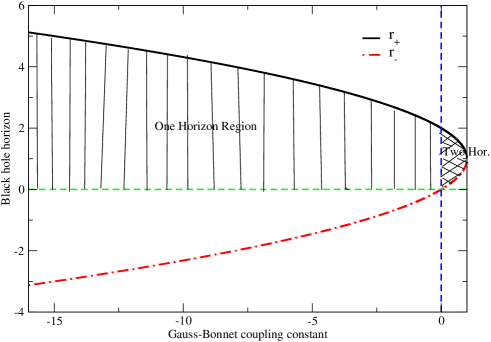
Figure 1: Black hole horizon radius $r_{+}$ and $r_{-}$ as a function of the Gauss-Bonnet coupling constant $\alpha$.

3 General Relativistic Hydrodynamical Equations

General Relativistic Hydrodynamics (GRH) is a necessary theory to understand the dynamic structures of the accretion disks around the black holes especially inside the region, $r<100M$ where the strong gravitational field is encountered. Here, $M$ is the mass of the black hole. The covariant forms of the GRH equations are in the following form (Donmez, 2004, 2006),

$$\bigtriangledown_{\mu}T^{\mu\nu}=0,\;\;\;\;\;\;\;\;\;\;\bigtriangledown_{\mu}J^{\mu}=0,$$ (5)

where $T^{\mu\nu}$ and $J^{\mu}$ are the stress-energy tensor and the matter current density, respectively. The latin indices run from $1$ to $3$ and Greek indices run from $0$ to $3$. In order to define the characteristic waves of the GRH equation, we simplify them neglecting the magnetic field and any type of the viscosity. Therefore the stress-energy tensor for a perfect fluid is,

$$T^{\mu\nu}=\rho hu^{\mu}u^{\nu}+Pg^{\mu\nu},$$ (6)

where specific enthalpy $h=1+\epsilon+\frac{P}{\rho}$. $\rho$, $P$, $u^{\mu}$, and $g^{\mu\nu}$ are the rest-mass density, ideal gas equation of state (pressure), four-velocity, and four metric, respectively. The equation of state is $P=(\Gamma-1)\rho\epsilon$. Here, $\Gamma$ is adiabatic index which defines the compressibility of the fluid.

The form of GRH equations given in Eq.5 is not suitable to use in High Resolution Shock Capturing scheme (HRSC). Hence, GRH equations are written in conservation form using $3+1$ formalism and we end up with the following first-order, flux-conservative hyperbolic system,

$$\frac{\partial\vec{U}}{\partial t}+\frac{\partial\vec{F^{i}}}{\partial x^{i}}=\vec{S},$$ (7)

where $\vec{U}$, $\vec{F^{i}}$, and $\vec{S}$ are conserved quantities, fluxes, and sources, respectively. Detailed formulations of these three vectors are given as the functions of lapse function $\tilde{\alpha}$, shift vectors $\beta^{i}$, the determinant of the three-metric $\gamma$, four-velocity $u^{\mu}$, three velocity $v_{i}$, Lorentz factor $W=\tilde{\alpha}u^{0}=(1-\gamma_{ij}v^{i}v^{j})^{-1/2}$, rest-mass density $\rho$, the components of the momentum vector $S_{i}$, pressure $P$, enthalpy $h$, and the $4D$ Christoffel symbol $\Gamma^{\alpha}_{\mu\nu}$. The spectral decomposition of the Jacobian matrix of the system $\partial\vec{F^{i}}/\partial\vec{U}$ is needed to use HRSC scheme and they are given in Donmez (2004) with the full details.

The static and spherically symmetric solution of the black hole in $4D$ Gauss-Bonnet gravity metric given in Eq.2 is used to define the source term appearing in the right hand side of Eq.7. The four-metric, three-metric, their inverses, the $4D$ Christoffel symbol, and Lorentz factor can be easily driven by having straightforward calculations. The lapse function for the EGB black hole is

$$\tilde{\alpha}=\left(1+\frac{r^{2}}{2\alpha}\left(1-\sqrt{1+\frac{8\alpha M}{r^{3}}}\right)\right)^{1/2},$$ (8)

and the shift vectors are,

$$\beta_{r}=0,\;\;\;\;\;\;\;\beta_{\phi}=0,\;\;\;\;\;\;\;\beta_{\theta}=0.$$ (9)

4 Bondi-Hoyle Accretion onto 4D EGB Black Hole

4.1 Theoretical Framework

A homogeneous supersonic flow that has a relative velocity $v_{\infty}$ and density $\rho_{\infty}$ at infinity is deflected by point mass $M$ due to the warped space-time (Hoyle & Lyttleton, 1939). The Bondi-Hoyle accretion condition for particles is defined with an impact parameter $\zeta$. As it is seen in Fig.2, if the pressure effect is negligible, the trajectory of the particle can be defined by conventional orbit. And then accretion condition is,

$$\zeta<\zeta_{HL}=\frac{2M}{v_{\infty}},$$ (10)

where $\zeta_{HL}$ is commonly known as accretion radius or the stagnation point. The suggested accreated matter could be computed by considering the trapped material inside the gravitational potential. The accretion rate suggested by Hoyle & Lyttleton (1939) is,

$$\dot{M}_{HL}=\pi\zeta^{2}_{HL}\rho_{\infty}v_{\infty}=\frac{4\pi M^{2}\rho_{\infty}}{v^{3}_{\infty}}.$$ (11)

The material falling towards the black hole that does not encounter to $\theta=0$ axis would not accreate and it would escape from the system as seen in dashed (blue) lines in Fig.2.

The theory given above does not exactly describe the motion of the gas flow accreated onto the black hole in the presence of the gas pressure in the strong gravitation region but it helps us define what the physical parameters are at infinity and how the accretion mechanism works.

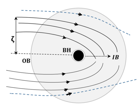
Figure 2: Artistic visualization of the Boyle Hoyle accretion around the black hole. BH $\equiv$ Black Hole, OB $\equiv$ Outer Boundary, and IB $\equiv$ Inner Boundary

Bondi-Hoyle accretion is studied in the vicinity of the Schwarzschild and Kerr black hole and called spherically symmetric accretion. During the accretion, the Bondi radius would be created and the accreated flow outside the radius is subsonic, and the disk mass-density is almost uniform. But the gas inside the radius becomes supersonic and it will be accreated towards to the black hole (Donmez et. al., 2011; Donmez, 2012). The strong gravity focuses the material behind the black hole (down-stream region) and the material would be accreated. In this paper, we will numerically model the Bondi-Hoyle accretion in the vicinity of the static and spherically symmetric black hole in $4D$ Gauss-Bonnet gravity to reveal the effect of Gauss-Bonnet coupling constant, not only on the shock cone structures but also on the oscillation properties and QPOs of those shock cones.

4.2 Initial and Boundary Conditions

Numerical simulation of the Bondi-Hoyle accretion around static and spherically symmetric non-rotating black hole defined in $4D$ EGB gravity gives us an opportunity to understand how the dynamics of the accretion disk and shock cone would be effected by the Gauss-Bonnet coupling constant $\alpha$. For this purpose, we numerically solve the GRH equations in spherical coordinate on the equatorial plane $(r,\phi)$, i.e. $\theta=\pi/2$ (see Eq.7) assuming spherical symmetry using the HRSC scheme based on approximate Riemann solver, further described in Donmez (2004).

As explained in section 3, we need to know pressure to evolve GRH equation depending on given initial values. The pressure is evaluated by using the perfect fluid equation of states $P=(\Gamma-1)\rho\epsilon$ with adiabatic index $\Gamma=4/3$. In order to perform the numerical simulation of the Bondi-Hoyle accretion on the equatorial plane, the gas is injected from an outer boundary of the upstream region with the following velocities,

$$V^{r}=\sqrt{\gamma^{rr}}V_{\infty}cos(\phi)\;\;\;\;\;\;\;\;V^{\phi}=-\sqrt{\gamma^{\phi\phi}}V_{\infty}sin(\phi)$$ (12)

$V_{\infty}$ is called the asymptotic velocity of the gas at infinity. The radial and angular velocities of the gas injected from the outer boundary are also given in terms of the components of the three-metric. The Eq.12 guarantees that $V^{2}=V_{i}V^{i}=V_{\infty}^{2}$ is valid everywhere along the computational domain.

The computational domain is defined on the equatorial plane with $r\in[r_{in},100M]$ and $\phi\in[0,2\pi]$ in spherical coordinate. The uniform grid is used in the all models along the radial and the angular directions with $N_{r}=1024$ $\times$ $N_{\phi}=512$ cells. So that the grid spacing is $(\triangle r,\triangle\phi)$ $=$ $(4.45\times 10^{-3}rad,9.4\times 10^{-2}M)$ in geometrized unit. We used the dynamical time step size in order to satisfy the Courant-Friedrich-Lewy stability condition. In order to extract the resolution dependencies of the numerical results, we monitor the the mass-accretion rate result from one of our initial condition, changing grid resolution. We explore the results from three different resolutions, $N_{r}=512$ $\times$ $N_{\phi}=256$, $N_{r}=1024$ $\times$ $N_{\phi}=512$, and $N_{r}=2048$ $\times$ $N_{\phi}=512$ and found that the oscillation amplitude of the mass-accretion rate slightly decreases with increasing employed resolution. But the observed trend is true for all initial conditions. So that the important outcome of this paper, effects of Gauss-Bonnet coupling constant $\alpha$ in $4D$ EGB gravity on the accreated matter and shock cones created around the black hole, would not be effected from the resolutions.

In order to model the Bondi-Hoyle accretion numerically, a homogeneous supersonic flow is injected from the upstream region $[\pi/2,3\pi/2]$ at the location of the outer boundary using the same analytic prescriptions given in Eq.12. The computational domain is extended from $r_{min}$, reported in Table 1 for different models, to outer boundary $r_{max}=100M$ which is fixed for all models. $\phi$ goes from $0$ to $2\pi$. The sound speed and the rest-mass density are chosen as $c_{s,\infty}=0.1$ and $\rho_{\infty}=1$, respectively at the boundary. And then the gas pressure is computed using the expression $p=c_{s,\infty}^{2}\rho(\Gamma-1)/[\Gamma(\Gamma-1)-c_{s,\infty}^{2}\Gamma]$ accordingly (Donmez et. al., 2011). The asymptotic velocity is chosen as $V_{\infty}=0.3$ with the parameters mentioned above and given in Table 1.

Table 1: The physical parameters and times: Gauss-Bonnet coupling constant $\alpha$, the inner boundary location of computational domain $r_{in}$, time to need to create a fully formed shock cone $t_{critial}$ (required time for the steady state), and total simulation time $t_{total}$. $M$ is the mass of the black hole.

$\alpha(M^{2})$	$r_{in}(M)$	$t_{critical}(M)$	$t_{total}(M)$
$-12$	$5$	$\sim 1920$	$19838$
$-7$	$5$	$\sim 1900$	$25940$
$-5$	$3.7$	$\sim 1850$	$21500$
$-0.8$	$2.5$	$\sim 1825$	$17750$
$-0.01$	$2.2$	$\sim 1810$	$16470$
$-0.0001$	$2.2$	$\sim 1665$	$21945$
$0.8$	$2.1$	$\sim 1500$	$18300$
SCHW	$2.2$	$\sim 1650$	$17000$

The initial injected values of a wind flow are used at upstream region at the outer boundary. The continuation is needed to avoid matter reflected back towards the black hole at the outer boundary of the downstream region (from $3\pi/2$ to $\pi/2$) along the radial coordinate. It is treated simply by using the zeroth-order extrapolation for all primitive variables. The inner boundary of computational domain along the radial distance close to the black hole horizon is implemented by using outflow boundary condition, handled simply copying first values to ghost zones. Lastly, the periodic boundary condition is adopted along the $\phi$ direction.

4.3 Numerical Results and Discussion

In order to reveal the effects of Gauss-Bonnet coupling constant $\alpha$ on the accreated material and the creation of shock cone, we first focus on the injected matter from the upstream region of the computational domain. Later, we wait some time to shock cone reaching the steady state and it is called $t_{critical}$. The critical times are varying from $1500M$ to $1920M$, shown in Table.1. The evolution of these models are, at least, followed up to $t=16470M$ which is sufficient to extract oscillation properties of the shock cone after reaches the critical time. The critical time is getting smaller for $\alpha>0$ while it is increasing for $\alpha<0$.

The morphology of the accreated shock cones formed in downstream region are given for the various values of Gauss-Bonnet coupling constant $\alpha$, seen in Fig.3 where we report the logarithmic rest-mass density of the accreated matter. The snapshots refer to $t\sim 15000M$, which is much later than the critical time needed to reach the steady state. The results due to different $\alpha$ show a qualitatively similar behavior, although quantitative differences appear in all models. The development of the shock cone and its strong shock locations, also seen in Fig.6, could cause a chaotic non-linear phenomena inside the cone. The shock cones are attached to the numerical horizon, $r_{in}$ given in Table 1 for different values of $\alpha$. It is know that the certain amount of matter would pass across the cone and fall into the black hole.

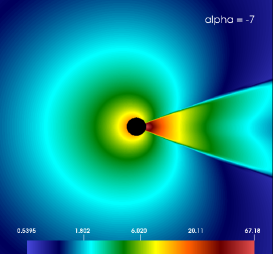
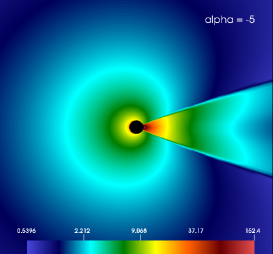
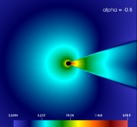
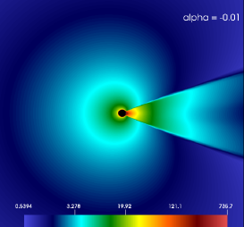
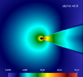
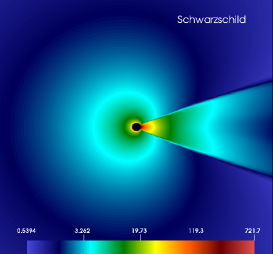
Figure 3: Close-up view of the snapshots of the logarithmic rest-mass density on the equatorial plane at $t\sim 15000M$ much later than the shock cone reached the steady state $t\sim 1900M$ for varying values of Gauss-Bonnet constant $\alpha$ and Schwarzschild black hole. The highlighted dynamic boundary is at $[x,y]$ $\rightarrow$ $[-70M,70M]$.

Besides, understanding the dynamic evolution of an accretion disk due to the Bondi-Hoyle accretion and calculating the mass accretion rates allow us to find out more important features of the shock cone. The mass accretion rate is,

$$\frac{dM}{dt}=-\int_{0}^{2\pi}\tilde{\alpha}\sqrt{\gamma}\rho u^{r}d\phi,$$ (13)

where all the physical quantities are defined in Section 3.

Here, we report the mass accretion rate at a fixed radial distance $r=6.1M$ for various values of $\alpha$. The mass accretion onto the $4D$ EGB black hole is clearly sensitive to the $\alpha$, as can be seen in Fig.4. It is clearly seen that increasing the value of $\alpha$ towards zero leads to more violent phenomena inside the shock cone and thus creates severe oscillations after the shock cone reaches the steady state. The high amplitude oscillation is an indicator of instability fully developed during the evolution. We have also confidence that the inner boundary of the computational domain does not play any role on oscillation properties of the shock cone. The oscillating properties of the mass accretion rates are not the same although the inner boundaries for $\alpha=-12$ and $\alpha=-7$ are in the same locations, On the other hand, oscillation inside the shock cone is considerably dissipated by the larger values of the negative $\alpha$.

The occurrence of the instability is the result of moving wave-like stretching into the medium which has a lower density. Overall, it is fair to say that, the instability inside the shock cone has been confirmed numerically, but it is still in debate whether the physical mechanisms driving the instabilities. The instability could be depended on the physical nature of the wind, such as sound speed, matter velocity, and Bondi accretion radius. A very detailed analysis of the unstable behavior of Bondi-Hoyle accretion flows was investigate by Foglizzo et. al. (2005), suggesting that the instability might be of adjective-acoustic nature in the case of shocks cones around the black hole.

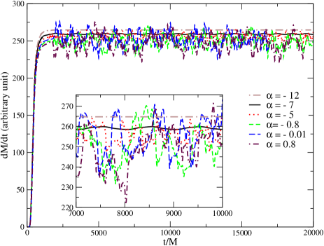
Figure 4: Mass accretion rate as a function of time for varying values of $\alpha$ at $r=6.1M$. The accretion rates reach the steady state around $t\simeq 1900M$ in all models.

After showing the behavior of the accretion rates in vicinity of $4D$ EGB black hole, we can now discuss the maximum value of oscillation strength using the mass accretion rate. Fig.5 represents the maximum oscillation amplitude $(\Delta\Phi)$ of the shock cone with various Gauss-Bonnet coupling constant $\alpha$ after the shock cone is fully formed. This is clear evidence that the significant oscillations happen when $\alpha$ is getting closer to zero as compared to high negative values. Together with the dependency of the accretion rate to $\alpha$, we have also investigated the convergence of EGB gravity solution to the general relativistic one. As it can be seen in Fig.5, $(\Delta\Phi)$ around the $4D$ EGB black hole converges to Schwarzschild one when $\alpha\rightarrow 0$.

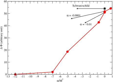
Figure 5: The behavior of the maximum oscillation amplitude $(\Delta\Phi)$ of the shock cone with varying Gauss-Bonnet coupling constant $\alpha$ after the shock cone is fully formed. Star seen in figure represents the oscillation amplitude of the shock cone around the Schwarzschild black hole.

To have deeper understanding of Fig.3, we extract the information along the angular direction $(\phi)$ at a fixed radial coordinate $r=6.5M$. The left panel of Fig.6 shows one-dimensional profiles of the rest-mass density for different values of Gauss-Bonnet coupling constant $\alpha$ and Schwarzschild solution. The strong shocks are created at the border of the shock cone. Therefore, a sharp transition is seen in density. The sharp transition location has a lowest density throughout the disk since along this location gas falls towards to the black hole along the streamlines, supersonically. The locations of streamlines seen in left side of the left panel of Fig.6 versus $\alpha$ are given in the right panel of the same figure. Increasing in $\alpha$ (going from $-7$ to $0.8)$ causes a slight exponential increase in the location of streamline, seen in the right panel of Fig.6. Hence the shock opening angle appeared in the downstream side of the computational domain expands along the angular direction.

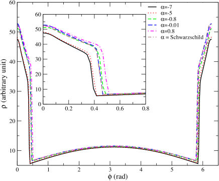
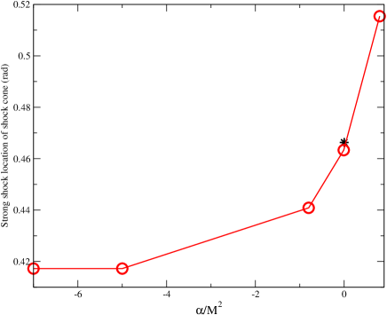
Figure 6: Left panel: The rest-mass density as a function of the angular coordinate $\phi$ at $r=6.5M$ for the varying values of the Gauss-Bonnet coupling constant $\alpha$ and Schwarzschild black hole. The embedded plots indicates the left shock locations to see the differences for varying $\alpha$. Right panel: The variation of the opening angle of the shock cone versus $\alpha$ computed at $\phi=\sim 0.5rad$ in left panel. The black star represents the location for the Schwarzschild black hole.

In order to uncover the effects of Gauss-Bonnet coupling constant $\alpha$ on the instability created during evolution and especially inside the shock cone after it reaches the steady state, we numerically study the Fourier mode analyze to compute the saturation point and to analysis the characterization of the instability. The Fourier mode $m=1$ is performed and the growth rates are obtained for the the rest-mass density power using the following equation (Donmez, 2014),

$$P_{m}=\frac{1}{r_{out}-r_{in}}\int_{r_{in}}^{r_{out}}{ln([Re(w_{m}(r))]^{2}+[Im(w_{m}(r))]^{2})dr},$$ (14)

where $r_{out}$ and $r_{in}$ are outer and inner boundary of the computational domain, respectively. The real and imaginary parts are $Re(w_{m}(r))=\int_{0}^{2\pi}\rho(r,\phi)cos(m\phi)d\phi$ and $Im(w_{m}(r))=\int_{0}^{2\pi}\rho(r,\phi)sin(m\phi)d\phi$.

As seen in Fig.7, the instability mode grows in the beginning of the simulation until $t\sim 304M$ for $\alpha=-7$ but the time is slightly getting greater when $\alpha$ converges to $0$. And then we have witnessed decreasing in the mode for a short time scale $(t\sim 200M)$. Later, the $m=1$ mode creates an exponential growth again until $t\sim 1400M$. The $m=1$ mode power reaches a maximum for the $\alpha$ getting close to zero and $0<\alpha<1$, although the modes in all models saturate almost at the same time $t\sim 1400M$. On the other hand, both $\alpha$ close to zero and Schwarzschild black hole power modes exhibit the same behavior during the evolution.

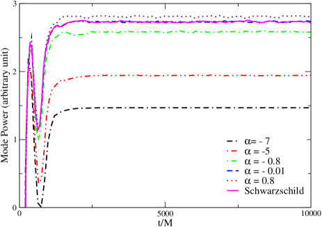
Figure 7: $m=1$ mode growth evolution around the EGB black hole for different values of $\alpha$ and Schwarzschild black hole. The region of interested is zoomed to see the saturation points and oscillations of the mode powers after they reached the steady state.

Fourier analysis of the computed data allows us to extract a lot of information about emerged phenomenology and their connections with Gauss-Bonnet coupling constant $\alpha$. In Fig.8, for instance, we obtain the power spectra using the rest-mass accretion rate computed during the time evolution for different values of $\alpha$ and Schwarzschild black hole. We have also conducted an extra test to find the dependency of power spectra to radial position and found that the mode of oscillation does not depend on the radial position. It means that the modes are global eigenmodes of the oscillating shock cone. As it is seen in Fig.8, there are two genuine eigenmodes appearing in the power spectra and the rest are the results of nonlinear couplings of these genuine modes. For Bondi-Hoyle accretion around the Schwarzschild solution, $f_{1}=9.5Hz$ and $f_{2}=17Hz$ are genuine eigenmodes, while $20Hz$, $27.7Hz$, $32Hz$, and $45.5Hz$ are the nonlinear couplings of those genuine eigenmodes with a $2Hz$ of error bar. These nonlinear couplings are $2f_{1}$, $3f_{1}$, $2f_{2}$, and $2f_{1}+f_{2}$, respectively. Similarly, for $\alpha=0.8$, $f_{1}=6Hz$ and $f_{2}=13.5Hz$ are genuine eigenmodes, while $21Hz$, $24Hz$, and $46.5Hz$ are the nonlinear couplings of those genuine eigenmodes with a $2Hz$ of error bar. These nonlinear couplings are $f_{1}+f_{2}$, $4f_{1}$, and $5f_{1}+f_{2}$, respectively. For $\alpha=-0.8$, $f_{1}=11Hz$ and $f_{2}=15.5Hz$ are genuine eigenmodes, while $36Hz$, $42Hz$, and $47.5Hz$ are the nonlinear couplings of those genuine eigenmodes with a $2Hz$ of error bar. These nonlinear couplings are $3f_{2}-f_{1}$, $f_{1}+2f_{2}$, and $3f_{2}$, respectively. For $\alpha=-5$, $f_{1}=30Hz$, $f_{2}=39.5Hz$, and $f_{3}=63Hz$ are genuine eigenmodes, while $49Hz$, $58.3Hz$, $78Hz$, and $89Hz$ are the nonlinear couplings of those genuine eigenmodes with a $2Hz$ of error bar. These nonlinear couplings are $2f_{2}-f_{1}$, $3f_{2}-2f_{1}$, $2f_{2}$, and $3f_{2}-f_{1}$, respectively. This behavior is expected behavior of the nonlinear equations in the physical system in the limit of small oscillations (Landau & Lifshitz, 1976). It is also important to note that the genuine modes and their nonlinear couplings show different behavior for $\alpha=-5$. There are three main differences between $\alpha$ close to zero (Schwarzschild solution) and negative value of $\alpha$ when $\alpha=-5$. First, there are two genuine modes for $-0.8\leq\alpha\leq 0.8$ while there are three for $\alpha=-5$. Second, the frequency of the first genuine mode $f_{1}$ is getting greater when $\alpha$ goes from $0.8$ to $-5$. Third, the frequencies of these genuine eigenmodes are much higher in $\alpha=-5$ than the other three cases. As it is expected, the amplitude of genuine modes are getting smaller when $\alpha$ is getting larger in negative direction.

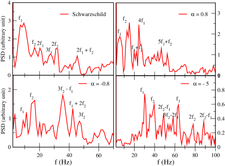
Figure 8: Power spectra of the mass accretion rate for different values of Gauss-Bonnet coupling constant $\alpha$ and Schwarzschild solution computed at $r=6.1M$. The mass of the black hole was assumed to be $M=10M_{\odot}$.

4.4 Comparison of 4D EGB and Schwarzschild Black Holes

To illustrate the consistency of the results found from the static spherically symmetric black hole solution in a novel $4D$ EGB gravity with the Schwarzschild one, the Schwarzschild solution of the Bondi-Hoyle accretion using the same initial conditions is performed. Fig.9 shows the comparison of the accretion rates between EGB and Schwarzschild solutions using certain values of the Gauss-Bonnet coupling constant $\alpha$. The accretion rates are plotted after the initial phase of relaxation of the shock cone. As it is also seen in the previous section, the computed accretion rate for the $\alpha=-0.0001$ shows similar behavior (oscillation + amplitude) with the Schwarzschild solution. Obviously, tendency of $\alpha$ to reach zero would give the solution in the general relativity. But decreasing in the parameter $\alpha$ causes a significant change in the oscillation properties of the accreated disk. So that a smaller $\alpha$ would cause to form a less luminous, cooler, and less efficient shock cone around the black hole. This is in agreement with a thin accretion solution around the $4D$ EGB black hole (Cheng et. al., 2020).

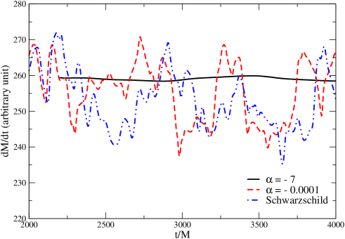
Figure 9: Comparison of the mass accretion rate for $\alpha=-7$ and $-0.0001$ with Schwarzschild solution as a function of time. The mass accretion rates are plotted after the shock cone reaches to the steady state.

Power spectrum data has a clear signature about the creation of shock cone instability for various values of Gauss-Bonnet coupling constant $\alpha$ and Schwarzschild black hole. Fig.10 represents how the maximum value of the $m=1$ power mode $(A_{mod}(max))$ changes with $\alpha$ and Schwarzschild black hole. $A_{mod}(max)$ increases with an increasing $\alpha$ and it goes to the Schwarzschild solution when $\alpha\rightarrow 0$ (e.g. see the star and the square symbols at $\alpha\sim 0$ in Fig.10). For the positive values of $\alpha$, it is seen in Fig.10 that increasing in $\alpha$ produces higher values of the maximum power spectrum.

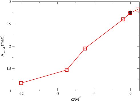
Figure 10: The maximum value of the $m=1$ power mode $(A_{mod}(max))$ versus Gauss-Bonnet coupling constant $\alpha$. Each value of power mode is extracted from the data after growth rate reaches to the saturation point. The star symbol represents the maximum power mode for the Schwarzschild black hole.

5 Conclusion

We have performed a systematic investigation of Gauss-Bonnet coupling constant $\alpha$ during the Bondi-Hoyle accretion onto a non-rotating black hole in $4D$ EGB gravity. The effect of $\alpha$ on the shock cone and its oscillation properties have been extensively studied when $-12\leq\alpha<1$. The numerical simulation of Bondi-accretion onto Schwarzschild black hole using the same initial condition is also performed to compare the general relativistic solution with $4D$ EGB gravity one.

We investigate how the physical features of the shock cone and its oscillation properties depend on $\alpha$ and find the following outcomes summarized in Table 2.

• We have found that the Bondi-Hoyle accretion around $4D$ EGB black hole with a negative Gauss-Bonnet coupling constant produces physical solution even it is very close to the black hole horizon. The same was also confirmed by Guo & Li (2020) for the geodesic motions of time-like and null particles.

• The numerical simulations reveal that moving matter from upstream side of the computational domain creates a steady state shock cone in a short time scale. The required time having the shock cone in downstream region is called critical time which decreases for $\alpha>0$ while increases for $\alpha<0$.

• The key indicator of having instability inside the shock cone is a high amplitude oscillation. The increase in the $\alpha$ that is getting close to zero, would lead to more violent phenomena inside the shock cone. Therefore the severe oscillations are created after the shock cone reaches the steady state. In addition, the oscillation inside the shock cone is considerably dissipated by the larger values of the negative $\alpha$.

• The shock opening angle slightly depends on the variation of $\alpha$. Going from $\alpha=-7$ to $\alpha=0.8$ would lead an exponential growth in the location of the shock cone.

• The power mode $m=1$ reaches a saturation point almost at the same time for all models. The $m=1$ mode power gets the maximum value when $\alpha$ is close to zero and $0<\alpha<1$. In addition, the power modes calculations for the Schwarzschild black hole and for $\alpha$ close to zero show the same behavior during the evolution.

Table 2: The effects of Gauss-Bonnet coupling constant $\alpha$ to the accretion mechanism, shock cones, and physical interpretation are summarized. $D$ represents decreasing while $I$ represents increasing. $SS$, $SC$, $PD$ stand for Steady State, Shock Cone , and Power Mode, respectively.

		Time to reach the SS
$\alpha=-12$	$\Longleftarrow(I)$	$\alpha=0$	$\Longleftarrow(I)$	$\alpha<1$
		Density inside the SC
$\alpha=-12$	$\Longleftarrow(D)$	$\alpha=0$	$\Longleftarrow(I)$	$\alpha<1$
		Max. PD after saturation
$\alpha=-12$	$\Longleftarrow(D)$	$\alpha=0$	$\Longleftarrow(D)$	$\alpha<1$
		The shock location
$\alpha=-12$	$\Longleftarrow(D)$	$\alpha=0$	$\Longleftarrow(D)$	$\alpha<1$

In addition to recovering many important features of the shock cones for varying $\alpha$, the novel features of the shock cones which traps the pressure modes inside the high density are also extracted by using Fourier transform. QPOs are computed for the Schwarzschild and different values of $\alpha$, i.e. $\alpha=0.8$, $\alpha=-0.8$, and $\alpha=-5$. The global genuine modes and their nonlinear oscillation counterparts are obtained in all cases. $\alpha$ influences not only the amplitude of modes but also their absolute frequencies of the trapped modes. There are three genuine modes found in $\alpha=-5$ while it is two for $\alpha=0.8$ and $\alpha=-0.8$ including the Schwarzschild one. It is also important to note that the higher absolute frequencies are found in case of $\alpha=-5$. As a result, having three genuine modes need to be confirmed by doing more accurate simulations in the negative $\alpha$ direction.

Possible applications of the numerical results discussed here could be Sagittarius $A^{*}$ (Sgr $A^{*}$) and High Mass $X-$ray Binaries (HMXBs). It is possible to have a direct comparison between numerically computed QPOs and QPOs observed in the $X-$ray spectra of these sources. Sgr $A^{*}$ black hole is located at the center of our own Galaxy and believed to be a supermassive black hole with a mass $4.6\pm 0.7\times 10^{6}M_{\sun}$ which is the one of target of Event Horizon Telescope (EHT) (Akiyama1 et. al., 2019; Akiyama2 et. al., 2019; Akiyama3 et. al., 2019; Abbott1 et. al., 2016; Abbott2 et. al., 2016). HMXBs are composed of black hole and of an OB star. We are planing to do more direct comparisons in the forthcoming paper. In this paper, we will investigate the effects of the black hole rotation parameter and Gauss-Bonnet coupling constant $\alpha$ on the shock cone dynamics around the rotating EGB black hole.

Finally, we have carried out a comparison of $4D$ EGB solution with Schwarzschild one. Obviously, it is seen from our numerical simulations that the tendency of $\alpha$ to reach zero would yield solution in general relativity.

References

- Akiyama1 et. al. (2019) K. Akiyama et al.[Event Horizon Telescope Collaboration], ApJ 875, L1 (2019).
- Akiyama2 et. al. (2019) K. Akiyama et al.[Event Horizon Telescope Collaboration], ApJ 875, L2 (2019).
- Akiyama3 et. al. (2019) K. Akiyama et al.[Event Horizon Telescope Collaboration], ApJ 875, L3 (2019).
- Abbott1 et. al. (2016) B. P. Abbott et al., Phys. Rev. Lett. 116, 061102 (2016).
- Abbott2 et. al. (2016) B. P. Abbott et al., Phys. Rev. Lett. 116, 221101 (2016).
- Frank et. al. (2002) J. Frank, A. King, & D. Raine, in Accretion Power in Astrophysics, 3rd ed. (Camebridge University Press, 2002).
- Yuan & Narayan (2014) F. Yuan & R. Narayan, Annu. Rev. Astron. Astrophys 52, 529 (2014).
- Nampalliwar & Bambi (2019) S. Nampalliwar & C. Bambi, Accreting Black Holes (2019), Tutorial Guide to X-ray and Gamma-ray Astronomy pp 15-54, arXiv: 1810.07041 [astro-ph].
- Glavan & Lin (2020) D. Glavan & C. Lin, Phys. Rev. Lett. 124, 081301 (2020).
- Cheng et. al. (2020) Cheng Liu, Tao Zhu & Qiang Wu, arXiv:2004.01662 [gr-qc].
- Julio et. al. (2020) Julio Arrechea, Adria Delhom, & Alejandro Jimenez-Cano 2020, arXiv:2004.12998 [gr-qc].
- Gurses et. al. (2020) M. Gurses, T. C. Sisman, & B. Tekin, Phys. Rev. Lett. 125, 149001 (2020).
- Ai (2020) W. Ai 2020, Commun. Theor. Phys. 72, 095402.
- Konoplya & Zinhailo (2020) R. A. Konoplya & A. F. Zinhailo, Physics Letters B 810, 135793 (2020).
- Roy & Chakrabarti (2020) Rittick Roy & Sayan Chakrabarti, Phys. Rev. D 102, 024059 (2020).
- Guo & Li (2020) M. Guo & P. C. Li, The European Physical Journal C 80, 588 (2020).
- Zhang et. al. (2020) Y. P. Zhang, S. W. Wei & Y. X. Liu 2020, arXiv:2003.10960 [gr-qc].
- Ghosh & Maharaj (2020) S. G. Ghosh & S. D. Maharaj, Phys. Dark Univ. 30, 100687 (2020).
- Ghosh & Kumar (2020) S. G. Ghosh & R. Kumar 2020, arXiv:2003.12291 [gr-qc].
- Yang et. al. (2020) Jun-Jie Wan, Jing Chen, Jie Yang & Yong-Qiang Wang, European Physical Journal C, 80, 937 (2020).
- Jin et. al. (2020) X. Jin, Y. Gao, & D. Liu, IJMPD 29(09), 2050061 (2020).
- Islam et. al. (2020) S. U. Islam, R. Kumar & S. G. Ghosh, Journal of High Energy Physics, 27, 1 (2020).
- Feng et. al. (2020) Jia-Xi Feng, Bao-Min Gu & Fu-Wen Shu 2020, arXiv:2006.16751 [gr-qc].
- Clifton et. al. (2020) Timothy Clifton, Pedro Carrilho, Pedro G. S. Fernan-des, & David J. Mulryne, Phys. Rev. D, 102, 084005 (2020).
- Zahra (2020) Zahra Haghani, Phys. Dark Univ. 30, 100720 (2020).
- Zhang et. al. (2020) C. Y. Zhang, P. C. Li & M. Guo, The European Physical Journal C, 80, 874 (2020).
- Edgar (2004) Edgar R., New Astronomy Review, 48, 843 (2004).
- Tejeda & Aguayo-Ortiz (2019) Emilio Tejeda, Alejandro Aguayo-Ortiz, MNRAS, 487(3), 3607 (2019).
- Donmez et. al. (2011) O. Donmez, O. Zanotti, and L. Rezzolla, MNRAS, 412, 3, 1659-1668.
- Donmez (2012) O. Donmez, MNRAS, 426, 1533D (2012).
- Cruz-Osorio & Lora-Clavijo (2016) Cruz-Osorio A. & Lora-Clavijo F. D., MNRAS, 460, 3193 (2016).
- Cruz-Osorio et. al. (2017) Cruz-Osorio A., Sanchez-Salcedo F. J. & Lora-Clavijo F. D., M NRAS, 471, 3127 (2017).
- Orosz et. al. (2008) Orosz, J. a., Steeghs, D., McClintock, J. E., Torres, M.A. P., Bochkov, I., Gou, L., Narayan, R., Blaschak, M.,Levine, A. M., Remillard, R. a., Bailyn, C. D., Dwyer,M. M., & Buxton, M., Astrophys. J., 697(1), 573–591 (2008).
- Lora et. al. (2013) Lora-Clavijo, F. D., & Guzman, F. S., MNRAS, 429(4), 3144–3154 (2013).
- Boulware & S. Deser (2020) D. G. Boulware & S. Deser, Phys. Rev. Lett. 55, 2656 (2020).
- Donmez (2004) O. Donmez, ApSS 293, 323-354 (2004).
- Donmez (2006) O. Donmez, AM&C 181, 256-270 (2006).
- Hoyle & Lyttleton (1939) F. Hoyle & R. A. Lyttleton, Proc. Cam. Phil. Soc, 35, 405 (1939).
- Donmez (2014) O. Donmez, MNRAS, 438, 846 (2014).
- Foglizzo et. al. (2005) Foglizzo T., Galletti P., Ruffert M., 435 Astron. Astrophys., 397 (2005).
- Landau & Lifshitz (1976) Landau L. D., Lifshitz E. M. 1976, Mechanics, 1. Perga-mon Press, Oxford.