Search for Continuous Gravitational Waves from Scorpius X-1 in LIGO O2 Data

Abstract

We present the results of a search in LIGO O2 public data for continuous gravitational waves from the neutron star in the low-mass X-ray binary Scorpius X-1. We search for signals with $\approx$ constant frequency in the range 40-180 Hz. Thanks to the efficiency of our search pipeline we can use a long coherence time and achieve unprecedented sensitivity, significantly improving on existing results. This is the first search that has been able to probe gravitational wave amplitudes that could balance the accretion torque at the neutron star radius. Our search excludes emission at this level between 67.5  Hz and 131.5  Hz, for an inclination angle $44^{\circ}\pm 6^{\circ}$ derived from radio observations (Fomalont et al., 2001), and assuming that the spin axis is perpendicular to the orbital plane. If the torque arm is $\approx$ 26 km – a conservative estimate of the Alfvén radius – our results are more constraining than the indirect limit across the band. This allows us to exclude certain mass-radius combinations and to place upper limits on the strength of the star’s magnetic field. We also correct a mistake that appears in the literature in the equation that gives the gravitational wave amplitude at the torque balance (Abbott et al., 2017b, 2019a) and we re-interpret the associated latest LIGO/Virgo results in light of this.

AM short = AM, long = amplitude modulation, class = abbrev NS short = NS, long = neutron star, class = abbrev GW short = GW, long = gravitational wave, class = abbrev LMXB short = LMXB, long = low-mass X-ray binary, class = abbrev ScoX1 short = Sco X-1, long = Scorpius X-1, class = abbrev CW short = CW, long = continuous wave, class = abbrev MDC short = MDC, long = mock-data challenge, class = abbrev SFT short = SFT, long = short Fourier transform, class = abbrev Tmax short = $T_{\text{max}}$, long = maximum time lag, class = abbrev FAP short = FAP, long = false alarm probability, class = abbrev SSB short = SSB, long = solar system barycenter, class = abbrev SNR short = SNR, long = signal to noise ratio, class = abbrev GR short = GR, long = general relativity, class = abbrev BH short = BH, long = black hole, class = abbrev CMB short = CMB, long = cosmic microwave background, class = abbrev PSD short = PSD, long = power spectral density, class = abbrev RMS short = RMS, long = root mean square, class = abbrev LIGO short = LIGO, long = Laser Interferometer Gravitational-Wave Observatory, class = abbrev FFT short = FFT, long = Fast Fourier Transform, class = abbrev LHO short = LHO, long = LIGO Hanford Observatory, class = abbrev CBC short = CBC, long = compact binary coalescence, class = abbrev

1 Introduction

Fast spinning neutron stars are promising sources of continuous gravitational waves in the frequency range 20 Hz - 2 kHz. The emission is typically generated by a non-axisymmetry in the star with respect to its rotation axis. The simplest example is the presence of an equatorial ellipticity that deforms the star into a triaxial ellipsoid rotating around the principal moment of inertia axis (Jaranowski et al., 1998).

The strength of the gravitational wave signal is proportional to the ellipticity of the star. The maximum ellipticity that a neutron star could support before breaking has been estimated to lie in the $10^{-7}-10^{-5}$ range for neutron stars made of normal matter and a few orders of magnitude higher for exotic matter (Horowitz & Kadau, 2009; Johnson-McDaniel & Owen, 2013; Baiko & Chugunov, 2018; Gittins et al., 2020). The minimum ellipticity is harder to estimate: we expect some ellipticity due to magnetic deformation, but the precise value depends strongly on the assumed magnetic field strength and configuration (see for example Haskell et al., 2008; Mastrano et al., 2011; Suvorov et al., 2016). Woan et al. (2018) have argued for a minimum ellipticity $\sim 10^{-9}$ based on the spin-down of millisecond pulsars (due to either magnetic field effects or some other source of ellipticity such as crustal deformation).

For accreting neutron stars, the accretion process provides a potential additional source of asymmetry, particularly if accreting material is channeled unevenly onto the surface by the star’s magnetic field. This can lead to thermal and compositional gradients in the crust that generate a crustal ‘mountain’ (Bildsten, 1998; Ushomirsky et al., 2000; Haskell et al., 2006; Singh et al., 2020). Accretion-induced deformation of the star’s magnetic field might also result in asymmetries (Melatos & Payne, 2005; Vigelius & Melatos, 2009). Accretion could also drive the excitation of some kind of internal oscillation that results in gravitational wave emission (Andersson et al., 1999; Haskell, 2015). Uncertainty about the accretion process and the stellar response makes it hard to compute firm estimates for the expected size of the resulting ellipticities, but they could be large enough for the resulting gravitational wave emission to be detectable with the current generation of detectors (Lasky, 2015).

What effect might such a gravitational wave torque have on an accreting neutron star? It has long been noted (Papaloizou & Pringle, 1978; Wagoner, 1984) that neutron stars in low mass X-ray binaries, in spite of having accreted matter for millions of years, spin well below the maximum possible spin frequency (Cook et al., 1994; Haensel et al., 2009), with the fastest accreting neutron star spinning at 620 Hz (Hartman et al., 2003; Patruno & Watts, 2012; Watts, 2012; Patruno et al., 2017). Since gravitational wave torques scale with a high power of the frequency, as the spin rate increases, they naturally provide a mechanism that kicks-in more strongly than other mechanisms, preventing further spin-up. This has led to the idea of torque balance, where gravitational wave and accretion torques reach equilibrium, preventing further spin-up and ensuring continuous gravitational wave emission (Bildsten, 1998). Indeed Gittins & Andersson (2019) have shown that a synthetic population of neutron stars evolved without the gravitational wave torque contribution does not produce the observed spin distribution.

The accretion torque on a neutron star having mass $M$ is

$$N_{\rm{acc}}=\dot{M}\sqrt{GMr_{m}},$$ (1)

where $G$ is the gravitational constant, $r_{m}$ is the torque arm and $\dot{M}$ the accretion rate. The correct value to use for $r_{m}$ is not known a priori, but is typically assumed to be either the neutron star radius $R$ or the radius at which the star’s magnetic field starts to disrupt the accretion flow.

The maximum accretion luminosity is ${{GM\dot{M}}\over R}$. If some fraction $X$ of this is radiated away by an X-ray flux $F_{X}$ observed at a distance $d$, then

$$X{{GM\dot{M}}\over R}={4\pi d^{2}F_{X}}\rightarrow\dot{M}={1\over X}{{4\pi d^{2}F_{X}R}\over{GM}}.$$ (2)

The gravitational wave intrinsic amplitude $h_{0}$ at a distance $d$, for a gravitational wave signal at twice the spin frequency of the star (which is the case if the ellipticity is caused by a magnetic or crustal mountain) and balancing the accretion torque, is

$$h_{0}^{torq.bal.}=\sqrt{{{5G}\over{2\pi^{2}c^{3}}}{\dot{E}_{\textrm{GW}}\over{d^{2}f^{2}_{\textrm{GW}}}}}~{}~{}{\textrm{with}}~{}~{}\dot{E}_{\textrm{GW}}=\pi f_{\textrm{GW}}N_{\rm{acc}},$$ (3)

where $f_{\textrm{GW}}$ is the gravitational wave frequency. Substituting Eq. 1 and 2 in Eq. 3 one finds

$$\begin{split}&h_{0}^{torq.bal.}=\sqrt{{{10}\over{Xc^{3}}}{F_{X}R\over{f_{\textrm{GW}}}}\sqrt{{Gr_{m}}\over M}}=\\ &=3.4\times 10^{-26}\left(\frac{1.4\,M_{\odot}}{M}\right)^{\frac{1}{4}}\left(\frac{r_{m}}{10\,\text{km}}\right)^{\frac{1}{4}}\times\\ &\times\left(\frac{F_{X}/X}{3.9\times 10^{-7}\,\text{erg}~{}\text{cm}^{-2}\text{s}^{-1}}\right)^{\frac{1}{2}}\left(\frac{R}{10\,\text{km}}\right)^{\frac{1}{2}}\left(\frac{600\,\text{Hz}}{f_{\text{GW}}}\right)^{\frac{1}{2}}.\end{split}$$ (4)

We note that Eq. 15 in Abbott et al. (2019a) and Eq. 10 in Abbott et al. (2017b) are incorrect and yield the correct numerical value only if $r_{m}=R$. In those papers such mistake propagates to the Alfvén radius torque balance amplitude curve of Fig. 5 (yellow curve in Abbott et al. 2019a), which is over-estimated. This in turn makes it look like the constrained inclination angle upper limits from that search (for $\iota=\iota_{\textrm{orb}}\ \approx 44^{\circ}$) probe the Alfvén radius torque balance limit, when in fact they do not.

For ease of notation we define

$$\begin{cases}M_{1}=\left({M}\over{1.4\,M_{\odot}}\right)\\ R_{1}=\left(\frac{R}{10\,\text{km}}\right)\\ r_{m1}=\left(\frac{r_{m}}{10\,\text{km}}\right)\\ B_{1}=\left({{B}\over{10^{9}~{}\textrm{G}}}\right)\\ f_{\textrm{GW}_{1}}=\left(\frac{f_{\text{GW}}}{600\,\text{Hz}}\right)\\ F_{X1}=\left(\frac{F_{X}}{3.9\times 10^{-7}~{}\text{erg}~{}\text{cm}^{-2}\text{s}^{-1}}\right)\\ d_{1}=\left(d\over{2.8\text{kpc }}\right)\\ \end{cases}$$ (5)

and re-write Eq. LABEL:eq:h0Torque as

$$\begin{split}h_{0}^{torq.bal.}=&\,3.4\times 10^{-26}\,X^{-{1\over 2}}\\ &M_{1}^{-{1\over 4}}\,{r_{m1}}^{\frac{1}{4}}\,{{F_{X}}_{1}}^{\frac{1}{2}}\,{R_{1}}^{\frac{1}{2}}\,{{f_{\text{GW}}}_{1}}^{-{1\over 2}}.\end{split}$$ (6)

ScoX1 is the brightest persistent X-ray source after the Sun and hence, given the scaling of gravitational wave amplitude with X-ray flux, it is a particularly promising continuous wave source. The flux value of ${3.9\times 10^{-7}\,\text{erg}/\text{cm}^{2}/\text{s}}$ used in Eq. LABEL:eq:h0Torque is the long-term average X-ray luminosity of ScoX1 measured from Earth (see Watts et al., 2008, for details of how this value was derived). This value yields a torque balance $h_{0}$ well within the reach of searches for continuous waves from known pulsars (Abbott et al., 2019b, 2020; Nieder et al., 2019, 2020).

Many searches have targeted continuous gravitational wave emission from ScoX1 (Meadors et al., 2017; Abbott et al., 2017a, c, d, 2019a, only since 2017), but none have yet been sensitive enough to probe the torque balance amplitudes of Eq. LABEL:eq:h0Torque. This is because in contrast to the known pulsars targeted in Abbott et al. (2019b, 2020); Nieder et al. (2019, 2020), the rotation frequency and frequency derivative of the ScoX1-neutron star, as well as some binary parameters, are unknown. This means that a broad range of waveforms must be tested against the data, and this degrades the attainable sensitivity, through the increased trials factor.

Another aspect that makes the ScoX1 signal search challenging is its computational cost: as illustrated in Watts et al. (2008) our ignorance of the system parameters results in a parameter space so broad that the most sensitive search method, a coherent matched filter over the entire observation time, is computationally prohibitive. This is a frequent predicament in searches for continuous gravitational waves and the standard solution is to adopt semi-coherent search methods, where one trades sensitivity in favour of computational efficiency (Messenger et al., 2015; Dergachev & Papa, 2019).

In semi-coherent searches the observation time is partitioned in segments spanning the same duration. If data from several instruments is used, these partitions are $\approx$ coincident in time. The most important quantity is the duration of such partitions, $T_{\textrm{coh}}$. The larger $T_{\textrm{coh}}$ is, the more sensitive and the more computationally expensive the search is going to be.

We use for this search a cross-correlation method (Whelan et al., 2015, and references therein). Thanks to the much improved computational efficiency of our new search (Meadors et al., 2018), we are able to use a significantly longer $T_{\textrm{coh}}$ than ever used before and reach unprecedented levels of sensitivity. In particular for the first time a search is sensitive to signals at the torque balance limit at both the stellar radius and for reasonable estimates of the magnetospheric radius.

2 The Search

We use LIGO O2 open data from the Hanford and Livingston detectors (LIGO, 2019; Vallisneri et al., 2015) between GPS time 1167984930  (January 2016) and GPS time 1187733514  (August 2016). Overall we have 5090 hours of data, 2496  from Livingston and 2594  from Hanford.

We search for a nearly monochromatic signal from the neutron star in ScoX1 – below we qualify this assumption further. At the detector the signal appears frequency-modulated due to the relative motion between the star and the detector, and amplitude-modulated due to the sensitivity-response of the detectors, which depends on the line-of-sight direction and hence for a fixed source changes with time. If all the source parameters were known, the gravitational waveform at the detector would also be known, and the search would be a perfectly matched filter, like those carried out for known pulsars. This is not the case.

The LMXB ScoX1 consists of a $1.4_{-0.5}^{+1.4}M_{\odot}$ neutron star and a $0.7_{-0.3}^{+0.8}M_{\odot}$ companion star (Wang et al., 2018, 95% confidence intervals). No accretion-powered pulsations or thermonuclear burst oscillations have been so far detected from the neutron star, so its spin frequency is unknown. The orbital parameters projected semi-major axis, $a\sin{i}$, time of ascending nodes, $T_{\rm{asc}}$, and orbital period, $P_{\rm{orb}}$, are constrained within ranges larger than our search resolution on those parameters, so these need to be explicitly searched (Wang et al., 2018).

The search parameters are given in Table 1. We search for gravitational wave signal frequencies between 40 Hz and 180 Hz. The computational cost per unit frequency interval is smaller at lower frequencies, so concentrating computational resources in the lower frequency range makes for the highest return in sensitivity. In fact this is the frequency range in which we can match the torque balance limit, even with an unrestricted prior on the star’s inclination angle.

We do not explicitly search over frequency derivatives, reflecting the assumption that the system is close to equilibrium. With our search set-up we have measured an average loss in SNR at the 15% level for gravitational wave first frequency derivative $|\dot{f}_{\textrm{GW}}|\simeq 2\times 10^{-13}$ Hz/s. This sets the scale for the maximum rate of change of the spin frequency that would not affect our ability to detect a signal, at $|\dot{f}_{\textrm{spin}}|\lesssim$ $1\times 10^{-13}$ Hz/s. We recall that for crustal mountains $f_{\textrm{GW}}=2f_{\textrm{spin}}$.

The orbital parameter ranges are taken from Table 2 of Wang et al. (2018). $T_{\rm{asc}}$ is propagated to 1178556229  GPSs which is $\approx$ the weighted middle of the LIGO data observation span. We note that this is 206 epochs after the $T_{\rm{asc}}$ in (Abbott et al., 2019a). Following Eq. 5 of Galloway et al. (2014), we expand the uncertainty associated with $T_{\rm{asc}}$ to 139  seconds and then consider the 3$\sigma$ confidence interval.

The grid spacings in every dimension $d\lambda$ are chosen so that the loss due to signal-template mismatch is at the $m=25\%$ level. The spacings are estimated based on the metric $g_{\lambda\lambda}$ as $d\lambda=\sqrt{\frac{m}{{g_{\lambda\lambda}}}}$. Expressions for the metric can be found in Whelan et al. (2015). This approach results in an overestimate of the actual mismatch (Allen, 2019), and in fact we measure an overall average SNR loss of 16%. The grid spacings are given in Table 1.

Our search employs a fixed $T_{\textrm{coh}}\simeq 19$ hrs, which is a factor of $4.5$ (10) longer than the longest (shortest) baseline used by Abbott et al. (2017e). This choice, enabled by the efficiency of our code (see Section 1) is the reason for the higher sensitivity of our search.

Table 1: Waveform parameter ranges

Parameter	Range	Grid spacing
$f_{\textrm{GW}}$ (Hz)	$[40,180]$	$\sim 2\times 10^{-6}$
$a\sin i$ (lt-s)	$[1.45,3.25]$	$\sim\frac{0.17~{}[{\textrm{lt-s}\,{\textrm{Hz}}}]}{f_{\textrm{GW}}}$
$T_{\text{asc}}$ (GPS s)	$1178556229\pm 3\times 139$	$\sim\frac{1576\,[{\textrm{lt-s}}]}{f_{\textrm{GW}}\,a\sin i}$
$P_{\text{orb}}$ (s)	$68023.86\pm 3\times 0.04$	$\sim\frac{18\,[{\textrm{lt-s}}]}{f_{\textrm{GW}}\,a\sin i}$

.

We consider search results with detection statistic values above the expected Gaussian-noise fluctuations. Since the number of searched waveforms increases with frequency, noise fluctuations alone produce higher fluctuations at higher frequencies. For this reason our threshold for candidate consideration is not constant but rather increases with frequency.

We find over 97 million results above the threshold. As often happens in this type of search, these results are not uniformly distributed in frequency but tend to come in groups, with the elements of each group having similar signal frequency, and due to the same root cause. We cluster these together and examine each cluster. We find 32  such groups, which we will refer to as “outlier clusters”. 23  of them are associated with known spectral contaminations (Covas et al., 2018). The rest of the clusters are discarded based on cross-checking the multi-detector detection statistics with the single-detector statistics: When an outlier is due to a disturbance in one of the detectors, the single-detector statistics will often be larger than the multi-detector one. On the contrary a signal produces a higher value when the data from both detectors is used. Most of these discarded clusters also present a range of signal frequencies with enhanced values of the detection statistic, that is much larger than it would be for a signal. The complete list of outlier clusters is given in Table 2.

3 Results

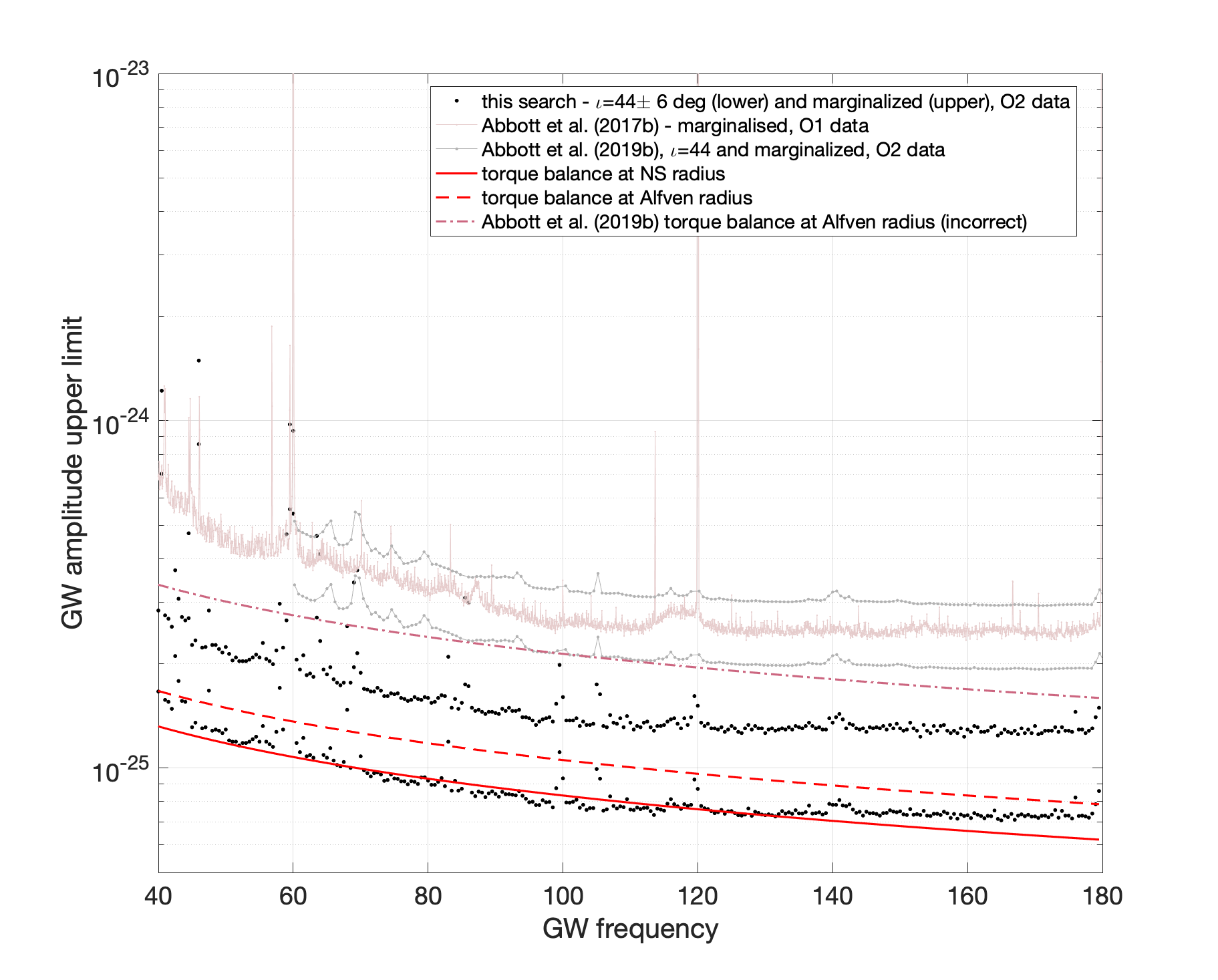
Figure 1: 95% confidence upper limits on the intrinsic gravitational wave amplitude in half-Hz bands. We assume orbital inclination at $44^{\circ}\pm 6^{\circ}$ (lower black points) and arbitrary inclination (upper black points). The lower dashed and solid curves are the torque-balance upper limits, based on estimates of the mass accretion rate and assuming the accretion torque to be at the neutron star radius (lower solid red curve) or at the Alfvén radius (upper dashed red curve). For comparison we show the upper limits from previous results (the three fainter upper curves) and draw the incorrect torque balance Alfvén radius upper limit that was reported (dash-dot line).

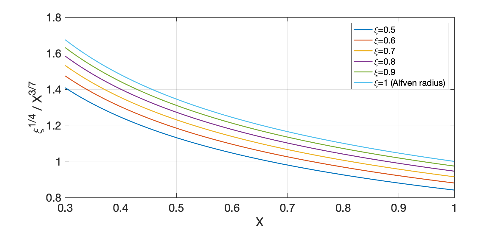
Figure 2: $h_{0}^{torq.bal.}(\xi,X)=h_{0}^{torq.bal.}(1,1){{\xi^{1/4}}\over X^{3/7}}$, and this multiplicative factor is shown here.

3.1 Upper limits on GW amplitude

As no significant candidate is found, we set upper limits at the 95% confidence level, on the gravitational wave intrinsic amplitude $h_{0}^{95\%}$ at the detectors, in half-Hz bands. The upper limits are determined by adding fake signals with a fixed amplitude $h_{0}$ to the data, and by measuring the detection efficiency, $C(h_{0})$. The detection criterion is determined by the value of the detection statistic of the most significant result in the band. The procedure is repeated for various values of $h_{0}$ and a sigmoid fit is used to determine the value corresponding to 95% confidence: $C(h_{0}^{95\%})=.95$ (Fesik & Papa, 2020).

Two sets of upper limits are derived, reflecting two assumptions: 1) an arbitrary value of the inclination angle, with $\cos\iota$ uniformly distributed $-1\leq\cos\iota\leq 1$, and 2) the inclination angle $\iota$ is equal to the orbital inclination angle and hence drawn from a Gaussian distribution with mean $44^{\circ}$ and standard deviation $6^{\circ}$ (Fomalont et al., 2001; Wang et al., 2018). The latter scenario is equivalent to assuming that the spin axis of the neutron star is perpendicular to the orbital plane. The $\iota=44^{\circ}\pm 6^{\circ}$ is a more favourable inclination than average for coupling to the gravitational wave detector (Jaranowski et al., 1998, see for instance Eq.s 21 and 22 ) and the resulting upper limits are a factor $\approx$ 1.7 smaller than those for arbitrary orientation.

Both upper limits are plotted in Fig. 1 and provided in machine-readable format in Zhang et al. (2020, and Suppl. Mat.). For comparison Fig. 1 also shows upper limits from a previous cross-correlation search on O1 LIGO data (Abbott et al., 2017d) and from a recent Viterbi algorithm search on the same O2 data that we use (Abbott et al., 2019a). The most sensitive of the two searches is the Abbott et al. (2017d) search. It employed variable coherence lengths, with longer ${T_{\textrm{coh}}}$ in the low frequency range, which explains why at lower frequency it is comparatively more sensitive than at higher frequency. The Abbott et al. (2019a) search is less sensitive than a cross-correlation search but is more robust to deviations of the signal waveform from the assumed model (Suvorova et al., 2016a, b). In particular the method of Abbott et al. (2019a) is robust with respect to loss of phase coherence in the signal.

One of the ways in which the signal could lose phase coherence with respect to the template waveforms of the search is through spin-wandering. This is a non-deterministic “jitter” in the spin of star, caused, for instance, by small changes in the mass accretion rate. The resulting frequency variation depends on the accretion torque, hence on the spin frequency of the star, its moment of inertia, the ratio between the torque arm and the co-rotation radius and the mass accretion rate.

Based on RXTE/ASM observations of Sco X-1, Mukherjee et al. (2018) have explored different system-parameter combinations and the gravitational wave frequency changes that may accumulate over different observation periods, due to spin wandering. Their results indicate that, in our frequency range, the maximum frequency change during an observation time of $2\times 10^{7}$ s (our observation time) is less than $2\,\mu$Hz (our frequency resolution) for the vast majority of the simulated systems. This means that the sensitivity of this search should not be impacted by spin-wandering effects.

Our results improve on existing ones by more than a factor $\approx$ 1.8. This is an extremely large sensitivity improvement in a large parameter space search like this one. For instance consider that in a broad all-sky search on O2 data, Abbott et al. (2019c) improve over the most sensitive results on O1 data (Dergachev & Papa, 2019) by a factor of $\approx$ 1.1.

3.2 Interpretation in terms of torque balance model

Our results are also remarkable in absolute terms because they probe gravitational wave amplitudes that could support emission at the torque balance level. It is the first time that this milestone is reached.

From Eq.s LABEL:eq:h0Torque or 6 we see that the torque balance gravitational wave amplitude depends on the torque arm and it is smallest at the star surface. If this minimum torque balance amplitude is larger than our $h_{0}^{95\%}$ upper limits it means that our search should have detected a signal; The fact that it has not, means that we can exclude such mass-radius combination:

$$[M_{1}^{-{1\over{4}}}R_{1}^{3\over 4}]^{\textrm{excl}}\geq{X^{1\over 2}}{{h_{0}^{95\%}}\over{3.4\times 10^{-26}}}f_{\textrm{GW}_{1}}^{\frac{1}{2}}F_{1}^{-{1\over 2}}.$$ (7)

The lower panel of Figure 4 shows the mass-radius regions excluded by the $\iota\approx 44^{\circ}$ gravitational wave upper limits for $f_{\text{GW}}=117.5$ Hz and $X=1$.

If the torque arm is larger than the star radius, the torque balance amplitude increases, and our gravitational wave upper limits constrain the magnetic field strength of the mass-radius combinations not excluded by 7. We illustrate this point in the next paragraphs.

We take the torque arm to be at the magnetospheric radius $r_{m}=\textrm{max}(\xi r_{A},R)$, with $0.5\leq\xi\leq 1$ and $r_{A}$ the Alfvén radius

$$r_{A}=25.6\,X^{2\over 7}\,{B_{1}}^{4\over 7}\,{R_{1}}^{10\over 7}\,{{M}_{1}}^{{1\over 7}}\,{{d}_{1}}^{-{4\over 7}}\,{{F_{X}}_{1}}^{-{2\over 7}}~{}{\textrm{km}},$$ (8)

where $B_{1}$ is the normalised polar magnetic field strength, defined in Eq. 5. We note that in the gravitational wave literature the Alfvén radius has often been placed at $35$ km, corresponding to $\dot{M}=10^{-8}\textrm{M}_{\odot}/\textrm{yr}$, or $X=0.3$ in Eq. 2. The Eddington limit is at $\dot{M}=2\times 10^{-8}\textrm{M}_{\odot}/\textrm{yr}$, for a fiducial 1.4 M_⊙ and 10 km radius neutron star.

By combining Eq. LABEL:eq:h0Torque and Eq. 8 we find the torque-balance amplitude when $r_{m}\geq R$:

$$\begin{cases}h_{0}^{torq.bal.}=&\,4.3\times 10^{-26}\,{{\xi^{1\over 4}}\over{X^{3\over 7}}}\\ &\times{{F_{X}}_{1}}^{3\over 7}\,{M_{1}}^{-{3\over{14}}}\,{R_{1}}^{6\over 7}\,{B_{1}}^{1\over 7}\,{d_{1}}^{-{1\over 7}}{f_{\textrm{GW}_{1}}}^{-{1\over 2}}\\ B_{1}\geq&0.19d_{1}\xi^{-7/4}(F_{1}/X)^{1/2}(R_{1}^{3}M_{1})^{-1/4},\\ \end{cases}$$ (9)

the last equation simply reflecting the condition $r_{m}\geq R$. We note that $h_{0}^{torq.bal.}(\xi,X)=h_{0}^{torq.bal.}(1,1){{\xi^{1/4}}\over X^{3/7}}$ and this factor is plotted in Fig. 2 to aid evaluate how the torque balance amplitude changes under different assumptions for torque arm $r_{m}$ and the accretion luminosity.

When this torque balance amplitude is larger than our $h_{0}^{95\%}$ upper limits it means that our search should have detected a signal; The fact that it has not, means that we can exclude the associated mass-radius-magnetic field strength combinations:

$$[M_{1}^{3\over{14}}R_{1}^{6\over 7}B_{1}^{1\over 7}]^{\textrm{excl}}\geq{{X^{3\over 7}}\over{\xi^{1\over 4}}}{{h_{0}^{95\%}}\over{4.3\times 10^{-26}}}f_{\textrm{GW}_{1}}^{\frac{1}{2}}F_{1}^{-{3\over 7}}d_{1}^{1\over 7}.$$ (10)

This translates, for every mass-radius, into an upper limit on the magnetic field strength.

Figure 4 shows the magnetic field upper limits from Eq. 10 from the $\iota\approx 44^{\circ}$ gravitational wave upper limits for $f_{\text{GW}}=117.5$ Hz, $X=1$ and $\xi=1$, for different equations of state. The upper limits for different gravitational wave frequencies can be easily derived from the gravitational wave upper limit values using Eq. 10. For the specific example shown in Figure 4, provided that the field is higher than $\sim 2\times 10^{8}$ G, the torque balance limit can be matched for all of the considered equations of state, but magnetic fields above $\sim 6\times 10^{8}$ G can be ruled out.

At Zhang et al. (2020, and Suppl. Mat.) we provide plots like the one of Figure 4 for gravitational wave frequencies in the searched range, at 2 Hz intervals.

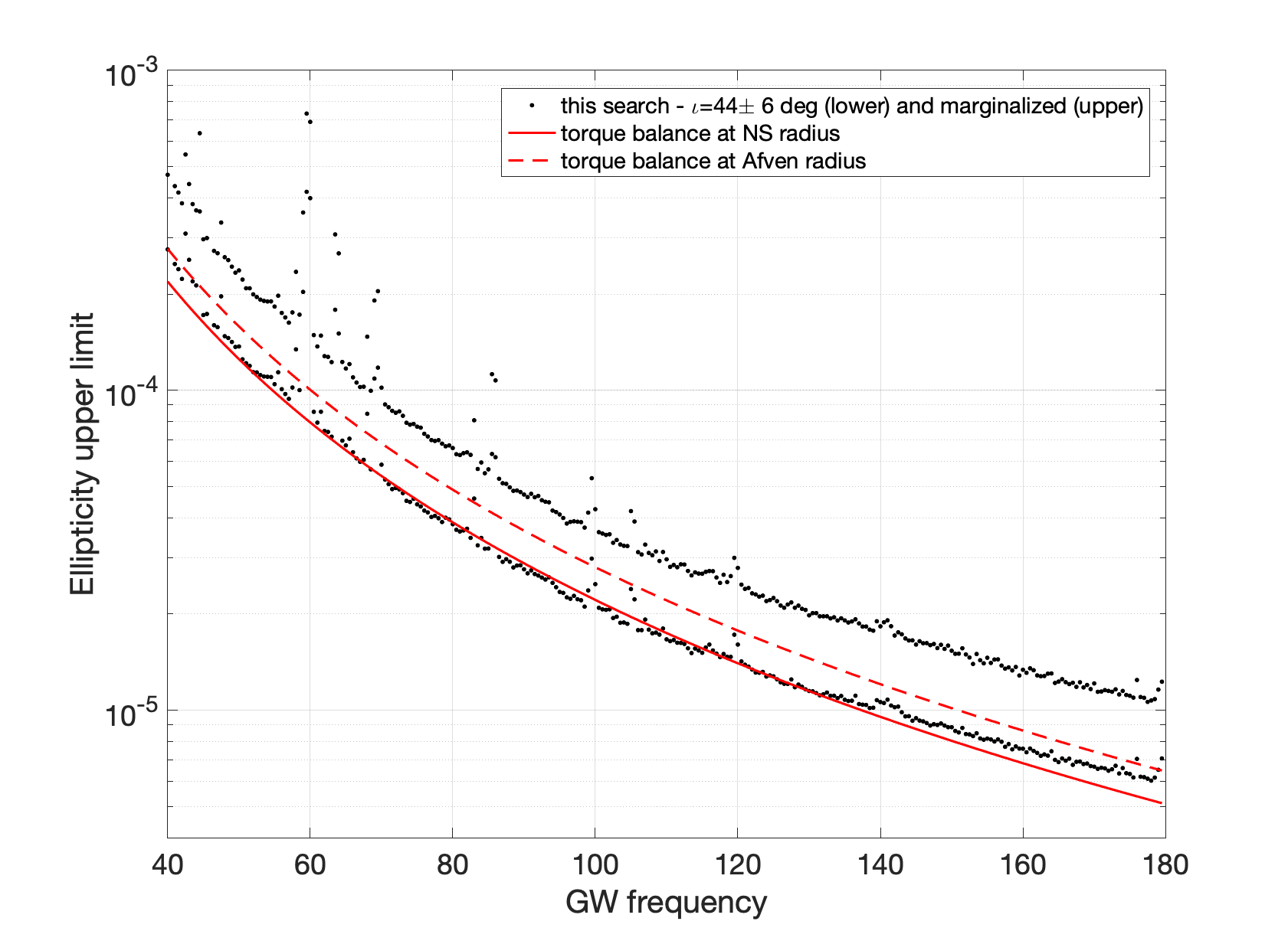
Figure 3: Upper limits on the ellipticity of the neutron star, derived from the gravitational wave intrinsic amplitude upper limits.

The gravitational wave upper limits marginalised over all possible inclination angles lead to less stringent constraints on the physical parameters of the neutron star: the torque balance amplitude with torque arm at the neutron star surface is smaller than our upper limits for all equations of state, so no mass-radius combination can be ruled out. Torque-balance amplitudes larger than our upper limits can only be obtained for larger torque arms corresponding to magnetic field strengths $\gtrapprox 10^{9}$ G, which are higher than those expected from LMXBs.

If the gravitational wave signal is due to a triaxial ellipsoid rotating around a principal moment of inertia axis $I$, say along the $\hat{z}$ axis, the gravitational wave intrinsic amplitude $h_{0}$ is proportional to the ellipticity $\varepsilon$ of the star:

$$\begin{cases}h_{0}=\frac{4\pi^{2}G}{c^{4}}{{I\varepsilon f^{2}_{\rm{GW}}}\over d}\\ \textrm{with}~{}~{}\varepsilon={{I_{xx}-I_{yy}}\over I}\end{cases}$$ (11)

We convert the $h_{0}^{95\%}$ upper limits into ellipticity upper limits with Eq. 11, with $d=2.8\text{kpc}$ and a fiducial value of $I=10^{38}\text{kg}~{}\text{m}^{2}$. We also derive the ellipticity required for torque balance under the two previous assumptions on the lever arm. All these quantities are plotted in Fig. 3, as a function of the gravitational wave signal frequency.

Above $\sim$ 90 Hz the values of the ellipticity that we are exploring are a few $\times 10^{-5}$ and smaller. Deformations which are this large may be sustained by a neutron star crust (Johnson-McDaniel & Owen, 2013), although very recent work suggests that the maximum deformations may be smaller (Gittins et al., 2020).

4 Discussion

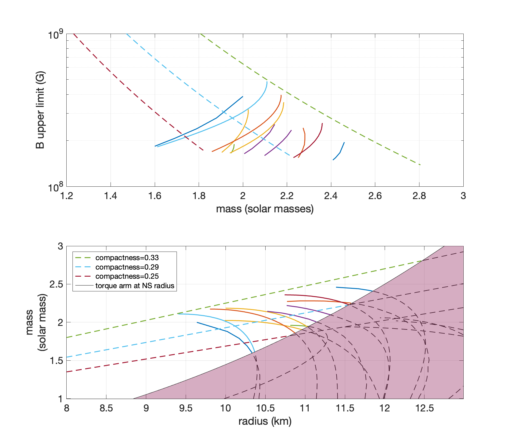
Figure 4: We have assumed $f_{\text{GW}}=117.5$ Hz ($\approx 17$ ms spin period), $\iota=44^{\circ}\pm 6^{\circ}$, $r_{m}=r_{A}~{}(\xi=1)$, $X=1$ and torque balance. Top panel: the largest magnetic field consistent with our null result. The solid lines correspond to the equations of state from Özel & Freire (2016, http://xtreme.as.arizona.edu/NeutronStars/index.php/dense-matter-eos/). The dashed lines indicate stars of constant compactness $GM/Rc^{2}$ equal to 0.33 (upper), 0.29 (middle) and 0.25 (lower). We have considered masses in the range 1 to 3 M_⊙, radii between 8 and 13 km and we have dropped any equation of state with a maximum mass lower than 1.9 M_⊙, consistent with observations (Antoniadis et al., 2013; Cromartie et al., 2019) and with estimates from dense matter theory and experiment, (see for example Hebeler et al., 2013; Kurkela et al., 2014). The lowest value of $B$ for each curve corresponds to $B(r_{m}=R)$. Lower panel: mass-radius relations for the equations of state considered above (solid lines) and for star configurations of constant compactness (dashed lines). The line that delimits the shaded region shows the mass-radius combinations that satisfy Eq. 7, i.e. that are consistent with our upper limits when $r_{m}=R$. Below the shaded region the torque balance gravitational wave amplitude with $r_{m}=R$, is larger than our upper limits, so these configurations are excluded by our null results. Above the shaded region the torque balance gravitational wave amplitude with $r_{m}=R$, is smaller than our upper limits, so these configurations cannot be excluded if $r_{m}=R$. If, however, $r_{m}>R$, i.e. a magnetic field above $\approx 2\times 10^{8}$ G, the corresponding torque balance becomes larger than our upper limits and this allows us to constrain the magnetic field (as shown in the top panel).

This search has placed upper limits on stable GW emission that are tighter than the level predicted by torque balance models for ScoX1, for $\iota\sim 44^{\circ}$. This conclusion is robust to spin wandering at the level expected for this source. If the accretion torque is applied at the neutron star surface, the GW frequency range for which the torque balance limit is beaten is between 67.5-131.5  Hz, for a 1.4 M_⊙ and 10 km radius fiducial star. If on the other hand the torque is applied at a magnetospheric radius at 25.6 km (see Eq.s 5 and 8), then the range for which the limit is beaten is the entire searched range, 40-180 Hz, for the fiducial star, as shown in Fig. 1.

If we consider a wider range of masses and radii, consistent with our current best understanding of viable equation of state models, we are able to place constraints on mass-radius-magnetic field strength combinations:

• independently of the magnetic field value, our results exclude certain mass-radius combinations. Our tightest limits come for spin periods of $\sim$ 21 ms ($f_{\textrm{GW}}\sim 96$ Hz, at twice the spin frequency) with a narrow range of allowed masses extending only between 1.9-2.2 M_⊙ and magnetic fields larger than $\sim 3\times 10^{8}$ G being ruled out for all considered equations of state.

• if the magnetic field is larger than $0.19d_{1}\xi^{-7/4}(F_{1}/X)^{1/2}(R_{1}^{3}M_{1})^{-1/4}$ ($r_{m}>R$) we can place upper limits on the magnetic field strength. The upper limit on the magnetic field is highest for the highest mass in the range. Stiffer equations of state have a smaller range of masses (and magnetic field strengths) for which balance can still be possible at the level of our upper limits, than softer equations of state. We find that the field must be smaller than $(4-10)\times 10^{8}$ G, depending on frequency (but excluding too disturbed frequency ranges, e.g. 60 Hz), for all equations of state models considered.

It is the first time that constraints on the magnetic field, mass and radius are obtained through continuous wave observations. This is interesting because the magnetic field is in general very poorly constrained and because observations like these probe mass-radius and magnetic fields through an entirely different mechanism than gravitational wave binary inspiral signals (see e.g. Abbott et al., 2019d; Capano et al., 2020).

If the spin of ScoX1 is such that it is in the range where the limit is beaten (half the GW frequency for mountain models) and torque balance applies, this means that GW emission is not strong enough to balance the assumed accretion torque. This implies that the accretion torque must be less strong than predicted by the models presented in this paper, which could happen if, for example, strong radiation pressure modifies the structure of the inner disk (Andersson et al., 2005) or due to the effect of winds (Parfrey et al., 2016).

The result also puts limits on the size of thermal/compositional crustal or magnetic mountains in ScoX1. Limits can also be placed on internal oscillation amplitude for models where that is the mechanism that provides the GW torque (for a different range of spin frequencies since the relationship between spin and GW frequency is different for mode models).

An alternative, of course, is that the spin of ScoX1 is outside the range searched, perhaps at higher frequencies more in line with the spin rates measured for the accretion-powered millisecond pulsars and thermonuclear burst oscillation sources (Patruno & Watts, 2012; Watts, 2012).

At 1 kHz the torque balance upper limit for the “fiducial star” is between 2.6-3.3 $\times 10^{-26}$, for $r_{m}\in[10-25.6]$ km. This is about a factor of 5-10 lower than a signal that we could detect at that frequency with a search like this one – the variation depending on the torque arm and on the inclination angle, and assuming that one could actually perform this search at such high frequencies. If all the parameters of ScoX1 were known, a search on the same O2 data as used here could probably detect signals at 2.6-3.3 $\times 10^{-26}$. We are however quite far from having a complete ephemeris for ScoX1. The next best thing would be to know the rotation frequency of the neutron star. The reason is that the torque balance amplitude decreases with frequency (so the sensitivity requirement increases, to match the torque balance limit), and the sensitivity of the searches decreases with frequency due to the shot noise in the detectors and to the increased template resolution per-Hz searched. These factors make it difficult to search very broad frequency bands. If it were possible to identify the spin frequency, for example via the detection of weak or intermittent pulsations (a major goal for future large-area X-ray telescopes Watts et al. 2019; Ray et al. 2019), we might be able to carry out a search like this one, that could begin to probe the torque balance limit when the noise level at 1 kHz reaches its design value of $\sim 5.5\times 10^{-24}\,1/\sqrt{\textrm{Hz}}$ (Abbott et al., 2018) and with $\sim$ two years of data.

5 ACKNOWLEDGMENTS

The computation of the work was run on the ATLAS computing cluster at AEI Hannover AEI (2017) funded by the Max Planck Society and the State of Niedersachsen, Germany. A.L.W. acknowledges support from ERC Consolidator Grant No. 865768 AEONS (PI: Watts).
This research has made use of data, software and/or web tools obtained from the LIGO Open Science Center (https://losc.ligo.org), a service of LIGO Laboratory, the LIGO Scientific Collaboration and the Virgo Collaboration. LIGO is funded by the U.S. National Science Foundation. Virgo is funded by the French Centre National de Recherche Scientifique (CNRS), the Italian Istituto Nazionale della Fisica Nucleare (INFN) and the Dutch Nikhef, with contributions by Polish and Hungarian institutes.

Appendix A Outlier table

Table 2: Table of outlier clusters, as described in the text.

Cluster ID	freq [Hz]	detection statistic	description
0	40.883985	180.55	known line in H1/L1 & too broad in freq.
1	42.852488	19.05	known line in H1/L1 & too broad in freq.
2	43.338994	12.99	fails single/multi-detector statistic comparison & too broad in freq.
3	44.524761	35.08	known line in H1/L1 & too broad in freq.
4	46.089393	415.72	fails single/multi-detector statistic comparison & too broad in freq.
5	47.679448	15.54	known line in H1/L1 & too broad in freq.
6	55.565183	11.96	known line in H1/L1
7	58.188448	17.06	fails single/multi-detector statistic comparison & too broad in freq.
8	59.516247	42.19	known line in H1/L1 & too broad in freq.
9	60.005969	185.90	known line in H1/L1 & too broad in freq.
10	61.814927	11.50	known line in H1/L1 & too broad in freq.
11	63.994606	68.80	known line in H1/L1 & too broad in freq.
12	64.025584	13.24	same as cluster 11 & too broad in freq.
13	64.279235	14.38	fails single/multi-detector statistic comparison & too broad in freq.
14	68.463375	21.05	known line in H1/L1 & too broad in freq.
15	68.492385	18.08	known line in H1/L1 & too broad in freq.
16	69.564208	41.68	known line in H1/L1 & too broad in freq.
17	69.649598	13.55	known line in H1/L1 & too broad in freq.
18	69.764916	16.83	known line in H1/L1 & too broad in freq.
19	83.301663	18.59	fails single/multi-detector statistic comparison & too broad in freq.
20	85.989651	43.63	known line in H1/L1 & too broad in freq.
21	99.332771	11.80	fails single/multi-detector statistic comparison
22	99.382711	11.54	fails single/multi-detector statistic comparison
23	99.984856	18.68	known line in H1/L1 & too broad in freq.
24	105.249255	15.40	fails single/multi-detector statistic comparison & too broad in freq.
25	105.467399	12.97	known line in H1/L1 & too broad in freq.
26	105.603586	13.66	known line in H1/L1 & too broad in freq.
27	119.886974	13.63	known line in H1/L1 & too broad in freq.
28	119.934821	13.04	known line in H1/L1 & too broad in freq.
29	120.002786	11.84	known line in H1/L1 & too broad in freq.
30	176.308216	13.28	fails single/multi-detector statistic comparison & too broad in freq.
31	179.994556	12.76	known line in H1/L1

References

- Abbott et al. (2017a) Abbott, B., et al. 2017a, Phys. Rev. D, 95, 122003, doi: 10.1103/PhysRevD.95.122003
- Abbott et al. (2018) —. 2018, Living Rev. Rel., 21, 3, doi: 10.1007/s41114-018-0012-9
- Abbott et al. (2019a) Abbott, B., Abbott, R., Abbott, T., et al. 2019a, Physical Review D, 100, doi: 10.1103/physrevd.100.122002
- Abbott et al. (2019b) Abbott, B., et al. 2019b, Astrophys. J., 879, 10, doi: 10.3847/1538-4357/ab20cb
- Abbott et al. (2019c) —. 2019c, Phys. Rev. D, 100, 024004, doi: 10.1103/PhysRevD.100.024004
- Abbott et al. (2017b) Abbott, B. P., et al. 2017b, Phys. Rev., D95, 122003, doi: 10.1103/PhysRevD.95.122003
- Abbott et al. (2017c) —. 2017c, Phys. Rev. Lett., 118, 121102, doi: 10.1103/PhysRevLett.118.121102
- Abbott et al. (2017d) —. 2017d, Astrophys. J., 847, 47, doi: 10.3847/1538-4357/aa86f0
- Abbott et al. (2017e) Abbott, B. P., Abbott, R., Abbott, T. D., et al. 2017e, The Astrophysical Journal, 839, 12, doi: 10.3847/1538-4357/aa677f
- Abbott et al. (2019d) Abbott, B. P., et al. 2019d, Phys. Rev. X, 9, 011001, doi: 10.1103/PhysRevX.9.011001
- Abbott et al. (2020) Abbott, R., et al. 2020. https://arxiv.org/abs/2007.14251
- AEI (2017) AEI. 2017, The Atlas Computing Cluster, https://www.aei.mpg.de/24838/02_Computing_and_ATLAS. https://www.aei.mpg.de/24838/02_Computing_and_ATLAS
- Allen (2019) Allen, B. 2019, Phys. Rev. D, 100, 124004, doi: 10.1103/PhysRevD.100.124004
- Andersson et al. (2005) Andersson, N., Glampedakis, K., Haskell, B., & Watts, A. L. 2005, MNRAS, 361, 1153, doi: 10.1111/j.1365-2966.2005.09167.x
- Andersson et al. (1999) Andersson, N., Kokkotas, K. D., & Stergioulas, N. 1999, Astrophys. J., 516, 307, doi: 10.1086/307082
- Antoniadis et al. (2013) Antoniadis, J., et al. 2013, Science, 340, 6131, doi: 10.1126/science.1233232
- Baiko & Chugunov (2018) Baiko, D. A., & Chugunov, A. I. 2018, MNRAS, 480, 5511, doi: 10.1093/mnras/sty2259
- Bildsten (1998) Bildsten, L. 1998, Astrophys. J. Lett., 501, L89, doi: 10.1086/311440
- Capano et al. (2020) Capano, C. D., Tews, I., Brown, S. M., et al. 2020, Nature Astron., 4, 625, doi: 10.1038/s41550-020-1014-6
- Cook et al. (1994) Cook, G. B., Shapiro, S. L., & Teukolsky, S. A. 1994, ApJ, 423, L117, doi: 10.1086/187250
- Covas et al. (2018) Covas, P., et al. 2018, Phys. Rev. D, 97, 082002, doi: 10.1103/PhysRevD.97.082002
- Cromartie et al. (2019) Cromartie, H., et al. 2019, Nature Astron., 4, 72, doi: 10.1038/s41550-019-0880-2
- Dergachev & Papa (2019) Dergachev, V., & Papa, M. A. 2019, Phys. Rev. Lett., 123, 101101, doi: 10.1103/PhysRevLett.123.101101
- Fesik & Papa (2020) Fesik, L., & Papa, M. A. 2020, The Astrophysical Journal, 895, 11, doi: 10.3847/1538-4357/ab8193
- Fomalont et al. (2001) Fomalont, E., Geldzahler, B., & Bradshaw, C. 2001, Astrophys. J., 558, 283, doi: 10.1086/322479
- Galloway et al. (2014) Galloway, D. K., Premachandra, S., Steeghs, D., et al. 2014, Astrophys. J., 781, 14, doi: 10.1088/0004-637X/781/1/14
- Gittins & Andersson (2019) Gittins, F., & Andersson, N. 2019, Mon. Not. Roy. Astron. Soc., 488, 99, doi: 10.1093/mnras/stz1719
- Gittins et al. (2020) Gittins, F., Andersson, N., & Jones, D. 2020. https://arxiv.org/abs/2009.12794
- Haensel et al. (2009) Haensel, P., Zdunik, J. L., Bejger, M., & Lattimer, J. M. 2009, A&A, 502, 605, doi: 10.1051/0004-6361/200811605
- Hartman et al. (2003) Hartman, J. M., Chakrabarty, D., Galloway, D. K., et al. 2003, in AAS/High Energy Astrophysics Division #7, AAS/High Energy Astrophysics Division, 17.38
- Haskell (2015) Haskell, B. 2015, International Journal of Modern Physics E, 24, 1541007, doi: 10.1142/S0218301315410074
- Haskell et al. (2006) Haskell, B., Jones, D. I., & Andersson, N. 2006, MNRAS, 373, 1423, doi: 10.1111/j.1365-2966.2006.10998.x
- Haskell et al. (2008) Haskell, B., Samuelsson, L., Glampedakis, K., & Andersson, N. 2008, MNRAS, 385, 531, doi: 10.1111/j.1365-2966.2008.12861.x
- Hebeler et al. (2013) Hebeler, K., Lattimer, J. M., Pethick, C. J., & Schwenk, A. 2013, ApJ, 773, 11, doi: 10.1088/0004-637X/773/1/11
- Horowitz & Kadau (2009) Horowitz, C. J., & Kadau, K. 2009, Phys. Rev. Lett., 102, 191102, doi: 10.1103/PhysRevLett.102.191102
- Jaranowski et al. (1998) Jaranowski, P., Krolak, A., & Schutz, B. F. 1998, Phys. Rev. D., 58, 063001, doi: 10.1103/PhysRevD.58.063001
- Johnson-McDaniel & Owen (2013) Johnson-McDaniel, N. K., & Owen, B. J. 2013, Phys. Rev. D, 88, 044004, doi: 10.1103/PhysRevD.88.044004
- Kurkela et al. (2014) Kurkela, A., Fraga, E. S., Schaffner-Bielich, J., & Vuorinen, A. 2014, ApJ, 789, 127, doi: 10.1088/0004-637X/789/2/127
- Lasky (2015) Lasky, P. D. 2015, PASA, 32, e034, doi: 10.1017/pasa.2015.35
- LIGO (2019) LIGO. 2019, The O2 Data Release, https://www.gw-openscience.org/O2/, doi: 10.7935/CA75-FM95
- Mastrano et al. (2011) Mastrano, A., Melatos, A., Reisenegger, A., & Akgün, T. 2011, MNRAS, 417, 2288, doi: 10.1111/j.1365-2966.2011.19410.x
- Meadors et al. (2017) Meadors, G. D., Goetz, E., Riles, K., Creighton, T., & Robinet, F. 2017, Phys. Rev. D., 95, 042005, doi: 10.1103/PhysRevD.95.042005
- Meadors et al. (2018) Meadors, G. D., Krishnan, B., Papa, M. A., Whelan, J. T., & Zhang, Y. 2018, Phys. Rev., D97, 044017, doi: 10.1103/PhysRevD.97.044017
- Melatos & Payne (2005) Melatos, A., & Payne, D. J. B. 2005, ApJ, 623, 1044, doi: 10.1086/428600
- Messenger et al. (2015) Messenger, C., et al. 2015, Phys. Rev. D., 92, 023006, doi: 10.1103/PhysRevD.92.023006
- Mukherjee et al. (2018) Mukherjee, A., Messenger, C., & Riles, K. 2018, Phys. Rev. D, 97, 043016, doi: 10.1103/PhysRevD.97.043016
- Nieder et al. (2019) Nieder, L., et al. 2019, doi: 10.3847/1538-4357/ab357e
- Nieder et al. (2020) —. 2020. https://arxiv.org/abs/2009.01513
- Özel & Freire (2016) Özel, F., & Freire, P. 2016, Ann. Rev. Astron. Astrophys., 54, 401, doi: 10.1146/annurev-astro-081915-023322
- Papaloizou & Pringle (1978) Papaloizou, J., & Pringle, J. E. 1978, MNRAS, 184, 501, doi: 10.1093/mnras/184.3.501
- Parfrey et al. (2016) Parfrey, K., Spitkovsky, A., & Beloborodov, A. M. 2016, ApJ, 822, 33, doi: 10.3847/0004-637X/822/1/33
- Patruno et al. (2017) Patruno, A., Haskell, B., & Andersson, N. 2017, Astrophys. J., 850, 106, doi: 10.3847/1538-4357/aa927a
- Patruno & Watts (2012) Patruno, A., & Watts, A. L. 2012, arXiv e-prints, arXiv:1206.2727. https://arxiv.org/abs/1206.2727
- Ray et al. (2019) Ray, P. S., Arzoumanian, Z., Ballantyne, D., et al. 2019, arXiv e-prints, arXiv:1903.03035. https://arxiv.org/abs/1903.03035
- Singh et al. (2020) Singh, N., Haskell, B., Mukherjee, D., & Bulik, T. 2020, MNRAS, 493, 3866, doi: 10.1093/mnras/staa442
- Suvorov et al. (2016) Suvorov, A. G., Mastrano, A., & Geppert, U. 2016, MNRAS, 459, 3407, doi: 10.1093/mnras/stw909
- Suvorova et al. (2016a) Suvorova, S., Sun, L., Melatos, A., Moran, W., & Evans, R. J. 2016a, Phys. Rev. D, 93, 123009, doi: 10.1103/PhysRevD.93.123009
- Suvorova et al. (2016b) —. 2016b, Phys. Rev. D, 93, 123009, doi: 10.1103/PhysRevD.93.123009
- Ushomirsky et al. (2000) Ushomirsky, G., Cutler, C., & Bildsten, L. 2000, Mon. Not. R. Astron. Soc., 319, 902, doi: 10.1046/j.1365-8711.2000.03938.x
- Vallisneri et al. (2015) Vallisneri, M., Kanner, J., Williams, R., Weinstein, A., & Stephens, B. 2015, J. Phys. Conf. Ser., 610, 012021, doi: 10.1088/1742-6596/610/1/012021
- Vigelius & Melatos (2009) Vigelius, M., & Melatos, A. 2009, MNRAS, 395, 1972, doi: 10.1111/j.1365-2966.2009.14690.x
- Wagoner (1984) Wagoner, R. 1984, Astrophys. J., 278, 345, doi: 10.1086/161798
- Wang et al. (2018) Wang, L., Steeghs, D., Galloway, D. K., Marsh, T., & Casares, J. 2018, MNRAS, 478, 5174, doi: 10.1093/mnras/sty1441
- Watts et al. (2008) Watts, A., Krishnan, B., Bildsten, L., & Schutz, B. F. 2008, Mon. Not. R. Astron. Soc., 389, 839, doi: 10.1111/j.1365-2966.2008.13594.x
- Watts (2012) Watts, A. L. 2012, ARA&A, 50, 609, doi: 10.1146/annurev-astro-040312-132617
- Watts et al. (2019) Watts, A. L., Yu, W., Poutanen, J., et al. 2019, Science China Physics, Mechanics, and Astronomy, 62, 29503, doi: 10.1007/s11433-017-9188-4
- Whelan et al. (2015) Whelan, J. T., Sundaresan, S., Zhang, Y., & Peiris, P. 2015, Phys. Rev. D., 91, 102005, doi: 10.1103/PhysRevD.91.102005
- Woan et al. (2018) Woan, G., Pitkin, M. D., Haskell, B., Jones, D. I., & Lasky, P. D. 2018, ApJ, 863, L40, doi: 10.3847/2041-8213/aad86a
- Zhang et al. (2020) Zhang, Y., Papa, M. A., & Krishnan, B. 2020, Supplemental materials to the paper Search for Continuous Gravitational Waves from Scorpius X-1 in LIGO O2 Data, www.aei.mpg.de/continuouswaves/CrossCorr-O2-20-180