Neural Networks Optimally Compress the Sawbridge

Abstract

Neural-network-based compressors have proven to be remarkably effective at compressing sources, such as images, that are nominally high-dimensional but presumed to be concentrated on a low-dimensional manifold. We consider a continuous-time random process that models an extreme version of such a source, wherein the realizations fall along a one-dimensional “curve” in function space that has infinite-dimensional linear span. We precisely characterize the optimal entropy-distortion tradeoff for this source and show numerically that it is achieved by neural-network-based compressors trained via stochastic gradient descent. In contrast, we show both analytically and experimentally that compressors based on the classical Karhunen-Loève transform are highly suboptimal at high rates.

1 Introduction

Artificial Neural-Network (ANN)-based compressors have recently achieved notable successes on the task of lossy compression of multimedia, spanning an array of sources and in some cases outperforming compressors that have been extensively optimized (see, e.g., [1] and the references therein).

One explanation for the exemplary performance of ANNs is that it derives from their ability to approximate arbitrary functions (e.g., [2]), which in turn enables them to perform nonlinear dimensionality reduction [3]. To see this, first consider classical rate–distortion theory for Gaussian sources, which is based on linear dimensionality reduction [4, Sec. 4.5.2]. Specifically, one projects the source realization onto an orthogonal family of reconstructions obtained from the Karhunen-Loève Transform (KLT) of the source. One then quantizes the resulting coefficients, say with a uniform quantizer followed by entropy coding [5, Sec. 5.5]. At the decoder, the inverse transform is applied to the quantized coefficients. The size of the orthogonal family is generally less than the dimensionality of the source, which provides some amount of compression. The quantization process provides more. For Gaussian sources, this architecture is provably near-optimal at high rates [5, Sec. 5.6.2]. In particular, using a nonlinear transform in place of the KLT provides essentially no benefit.

For real-world multimedia sources, however, there is reason to believe that allowing for nonlinear transforms would be advantageous. The distribution of natural images is widely suspected to be supported by a low-dimensional manifold in pixel-space (e.g., [6]), for instance. That is, while the linear span of the manifold may be high, there exists a continuous, presumably nonlinear, map with a continuous, presumably nonlinear, inverse, from the manifold to a low-dimensional Euclidean space. One could in principle use such a map in place of the linear projections in the classical architecture, with the reduced dimensionality of the output afforded by allowing for nonlinear transforms translating to a lower bit-rate. State-of-the-art ANN-based compressors indeed follow this architecture, with nonlinear analysis and synthesis transforms surrounding a conventional uniform quantizer with entropy coding [1]. As a consequence, one might hypothesize that ANNs are particularly adept at compressing sources for which there is a large discrepancy between the amount of dimensionality reduction afforded by linear versus nonlinear transforms.

We provide evidence for this hypothesis by showing that ANNs optimally compress a prototypical source of this type, and that their performance beats the linear-transform-based approach by a large margin. We consider a particular stochastic process over $[0,1]$ that can be constructed from a continuous, nonlinear transformation of a single random variable. We learned of this process and its usefulness as a test-case for compression algorithms from the survey by Donoho et al. [7], who in turn credit Meyer [8]. Donoho et al. refer to this process as the Ramp; we shall call it the sawbridge. We focus on this process because it exposes the largest possible gap between linear and nonlinear dimensionality reduction. Donoho et al. point out that the sawbridge has the same autocorrelation, and thus the same KLT, as the Brownian bridge. In particular, the KLT of the sawbridge is infinite-dimensional. We show that any linear transform requires infinitely many components to recover the source. In contrast, there is a simple nonlinear transform that can recover the source realization from a one-dimensional projection.

We show that this discrepancy in dimensionality reduction translates to a large gap in compression performance. We analytically characterize the performance of optimal one-shot compression for the sawbridge and numerically show that it is realized by a deep ANN trained via stochastic gradient descent. We also characterize the performance of KLT-based schemes and show, both numerically and mathematically, that they are exponentially suboptimal.

The next section introduces the sawbridge process and its properties. Section 3 shows how to optimally compress the sawbridge. Section 4 characterizes the performance of schemes based on the KLT and entropy coding. Section 5 numerically shows that the sawbridge is optimally compressed by existing neural network architectures and training methods, and that linear-based methods are highly suboptimal. All proofs have been omitted due to space constraints but are available in the extended version of the paper [9].

2 The Sawbridge

The focus of this paper is the following stochastic process.

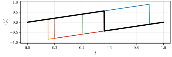
Figure 1: Realizations of the sawbridge. The bold line represents one full realization; others show additional samples.

Definition 1 (cf. [7]).

The sawbridge is the process

$$X(t)=t-\mathbf{1}(t\geq U)\quad t\in[0,1],$$ (1)

where $U$ is uniformly distributed over $[0,1]$. We use $X$ or $X(\cdot)$ to refer to the entire process $\{X(t)\}_{t=0}^{1}$.

See Fig. 1 for sample realizations. In words, the process jumps from the “rail” $t$ to the “rail” $t-1$ at the random time $U$. Alternatively, one can view $-X$ as the centered empirical cumulative distribution function of a single $\operatorname{unif}[0,1]$ random variable.

As noted in the introduction, we are interested in the sawbridge because it exposes the largest possible gap between the performance of linear and nonlinear dimensionality reduction. Call a map $f:L^{2}[0,1]\mapsto\mathbb{R}^{k}$ a transform (of dimension $k$) if it is continuous and there exists a continuous function $g:\mathbb{R}^{k}\mapsto L^{2}[0,1]$ (the inverse transform) such that

$$g(f(X))=X\quad\text{a.s.}$$ (2)

We call $\mathbb{R}^{k}$ the latent space.

If $f$ and, especially, $g$ are permitted to be nonlinear, then a transform of dimension one exists, which is clearly the lowest possible. Specifically, the choices

$$f(x)=\int_{0}^{1}x(t)\;dt$$ (3)

and

$$(g(y))(t)=t-\mathbf{1}(y\leq t-1/2)$$ (4)

suffice. This comports with the intuition that the process is completely described by $U$. In fact, the $f(\cdot)$ in (3) satisfies $f(X)=U-1/2$ a.s. if $X$ and $U$ are related by (1). Note that this $f$ happens to be a linear map.

On the other hand, if $f$ and $g$ are both required to be linear maps then (2) is impossible for any finite $k$. This follows from the following result on the Karhunen-Loève expansion of the process. Note that the sawbridge is zero mean and let

$$K(s,t)=E[X(s)X(t)]=\min(s,t)-st$$ (5)

denote its autocorrelation.

Theorem 1.

The functions

$$\phi_{k}(t)=\sqrt{2}\cdot\sin(\pi kt)\quad t\in[0,1],\quad k=1,2,\ldots,$$ (6)

form an orthonormal basis for $L^{2}[0,1]$. They are eigenfunctions of $K(\cdot,\cdot)$ with corresponding eigenvalues

$$\lambda_{k}=\frac{1}{\pi^{2}k^{2}},$$ (7)

meaning that

$$\int_{0}^{1}K(s,t)\phi_{k}(t)\;dt=\lambda_{k}\cdot\phi_{k}(s)$$ (8)

for all $k$ and $s\in[0,1]$. If we define

$$Y_{k} :=\int_{0}^{1}X(t)\phi_{k}(t)\;dt$$ (9)

$$=-\sqrt{2\lambda_{k}}\cos(\pi kU),$$ (10)

then $\{Y_{k}/\sqrt{\lambda_{k}}\}_{k=1}^{\infty}$ is a sequence of uncorrelated, zero-mean, unit-variance random variables such that the sawbridge can be written as

$$X(t)=\sum_{k=1}^{\infty}Y_{k}\phi_{k}(t),$$ (11)

in the sense that

$$\lim_{n\rightarrow\infty}\sup_{0\leq t\leq 1}E\left[\left(X(t)-\sum_{k=1}^{n}Y_{k}\phi_{k}(t)\right)^{2}\right]\;dt=0.$$ (12)

Proof.

It is straightforward to verify that $\{\phi_{k}(\cdot)\}_{k=1}^{\infty}$ forms an orthonormal family satisfying (8). To show that it forms an orthonormal basis for $L^{2}[0,1]$, consider any $g(\cdot)$ in $L^{2}[0,1]$ such that

$$\int_{0}^{1}g(t)\sin(\pi kt)\;dt=0\ \text{for all $k$.}$$ (13)

Consider the odd extension of $g(\cdot)$ to $[-1,1]$,

$$g_{o}(t)=\begin{cases}-g(-t)&\text{if $t\in[-1,0]$}\\ g(t)&\text{if $t\in(0,1]$}.\end{cases}$$ (14)

From (13), we have

$$\int_{-1}^{1}g_{o}(t)\sin(\pi kt)\;dt=0\quad k=1,2,3,\ldots.$$ (15)

At the same time, since $g_{o}(\cdot)$ is odd, we have

$$\int_{-1}^{1}g_{o}(t)\cos(\pi kt)\;dt=0,\quad k=0,1,2,\ldots.$$ (16)

The completeness of the Fourier basis implies that $g(\cdot)\equiv 0$ and hence $\{\phi_{k}(\cdot)\}_{k=1}^{\infty}$ is also an orthonormal basis (e.g., [10, Theorem 8.16], [11, Theorem 5.27]; note that the set of Riemann integrable functions is dense in $L^{2}$ [11, Prop. 6.7]). The rest of the conclusion then follows from the Karhunen-Loève theorem (e.g., [12, Prop. 4.1]; note that the sawbridge is quadratic-mean continuous, even though its realizations are obviously not continuous), except for (10), which follows by integrating (9) by parts. ∎

This implies that if the transform and inverse must be linear, then an infinite number of dimensions is required to represent the sawbridge, as shown in the following corollary.

Corollary 1.

For any finite $k$, if $f:L^{2}[0,1]\mapsto\mathbb{R}^{k}$ and $g:\mathbb{R}^{k}\mapsto L^{2}[0,1]$ are linear maps then they cannot satisfy (2).

Proof.

Suppose $f$ and $g$ are linear and let $Y=g(f(X))$. Then we can write

$$Y(t)=\sum_{i=1}^{k}A_{i}\psi_{i}(t)$$ (17)

for some random variables $A_{1},\ldots,A_{k}$ and orthonormal functions $\psi_{1}(\cdot),\ldots,\psi_{k}(\cdot)$. Then the autocorrelation of $Y$ has at most $k$ nonzero eigenvalues and hence $X$ and $Y$ have distinct distributions. ∎

The large gap between linear and nonlinear dimensionality reduction for the sawbridge has consequences for compression, to which we turn next.

3 Optimal Compression

We consider a one-shot form of compression in which the goal is to minimize the entropy of the compressed representation for a given mean squared error.

Definition 2.

An encoder is a map $f:L^{2}[0,1]\mapsto\operatorname{\mathbb{N}}$. Its entropy and distortion are

$$H(f) =-\sum_{i\in\operatorname{\mathbb{N}}}\operatorname{Pr}(f(X)=i)\log\operatorname{Pr}(f(X)=i)$$

$$D(f) =E\left[\int_{0}^{1}(X(t)-E[X(t)|f(X)])^{2}\;dt\right],$$

respectively.

Note that Definition 2 assumes that the reproduction $E[X(t)|f(X)]$ need not be a valid sawbridge realization. Also note that an encoder is distinct from a transform in that it maps the source realization to a discrete set and is therefore not invertible. In practice, compression involves mapping the source realization to a variable-length bit string, whose expected length one might wish to minimize. The minimum such expected length, $L^{*}(f)$, is known to satisfy $H(f)\leq L^{*}(f)<H(f)+1$ if one requires that the codewords are prefix-free (e.g., [13, Theorem 5.4.1]) and

$$L^{*}(f) \leq H(f)$$ (18)

$$H(f) \leq L^{*}(f)+(1+L^{*}(f))\log(1+L^{*}(f))-L^{*}(f)\log L^{*}(f),$$ (19)

if one does not [14, Theorem 1]. As such, it is reasonable to focus on $H(f)$ as the figure-of-merit, especially at high rates.

Definition 3.

The entropy-distortion function of the sawbridge is

$$H(\Delta)=\inf_{f}H(f),$$ (20)

where the infimum is over all encoders $f$ such that $D(f)\leq\Delta$.

Theorem 2.

If $\Delta\geq 1/6$, then $H(\Delta)=0$. For any $0<\Delta<1/6$, we have

$$H(\Delta)=-\left\lfloor\frac{1}{p}\right\rfloor\cdot p\log p-q\log q,$$ (21)

where $q=\left(1-\left\lfloor\frac{1}{p}\right\rfloor\cdot p\right)$ and $p$ is the unique number in $(0,1)$ such that

$$\left\lfloor\frac{1}{p}\right\rfloor\cdot p^{2}+q^{2}=6\Delta.$$ (22)

Proof.

If $\Delta\geq 1/6$, then a trivial encoder with a singleton range achieves $D(f)\leq\Delta$ and $H(f)=0$. Suppose $0<\Delta<1/6$. Each realization of $X$ can be identified with a unique realization of $U$, so the realizations of $X$ are in one-to-one correspondence with $[0,1]$. Thus for any encoder $f$ and any $i$, $f^{-1}(i)$ can be identified with a subset of $[0,1]$, say $A_{i}$, such that

$$E\left[\int_{0}^{1}(X(t)-E[X(t)|f(X)])^{2}\;dt\middle|f(X)=i\right]$$

$$=E\left[\int_{0}^{1}(X(t)-E[X(t)|U\in A_{i}])^{2}\;dt\middle|U\in A_{i}\right].$$

Now consider an arbitrary $A\subset[0,1]$ such that $\mu(A)>0$, where $\mu(\cdot)$ is the Lebesgue measure. We will show the inequality

$$E\left[\int_{0}^{1}(X(t)-E[X(t)|U\in A])^{2}\;dt\middle|U\in A\right]\geq\frac{\mu(A)}{6}.$$ (23)

To this end, note that we can write

$$E\left[\int_{0}^{1}(X(t)-E[X(t)|U\in A])^{2}\;dt\middle|U\in A\right]$$ (24)

$$=E\left[\int_{0}^{1}(\mathbf{1}(U\leq t)-E[\mathbf{1}(U\leq t)|U\in A])^{2}\;dt\middle|U\in A\right]$$ (25)

$$=\int_{0}^{1}\operatorname{Pr}(U\leq t|U\in A)(1-\operatorname{Pr}(U\leq t|U\in A))\;dt.$$ (26)

First suppose that $A$ is a union of intervals,

$$A=\cup_{i=1}^{k}[a_{i},b_{i}],$$ (27)

where $0\leq a_{1}<b_{1}\leq a_{2}<b_{2}\leq\ldots\leq a_{k}<b_{k}\leq 1$. Define

$$\beta_{0}=0\quad\text{and}\quad\beta_{i}=\sum_{\ell=1}^{i}\frac{b_{\ell}-a_{\ell}}{\mu(A)}$$ (28)

and note that $\beta_{k}=1$. Then from (26) we have

$$E\left[\int_{0}^{1}(X(t)-E[X(t)|U\in A])^{2}\;dt\middle|U\in A\right]$$ (29)

$$\geq\sum_{\ell=1}^{k}\int_{a_{\ell}}^{b_{\ell}}\operatorname{Pr}(U\leq t|U\in A)(1-\operatorname{Pr}(U\leq t|U\in A))\;dt$$ (30)

$$=\sum_{\ell=1}^{k}\int_{a_{\ell}}^{b_{\ell}}\left(\beta_{\ell-1}+\frac{t-a_{\ell}}{\mu(A)}\right)\left(1-\beta_{\ell-1}-\frac{t-a_{\ell}}{\mu(A)}\right)\;dt.$$ (31)

Performing the change of variable

$$s=\beta_{\ell-1}+\frac{t-a_{\ell}}{\mu(A)},$$ (32)

the quantity in (31) equals

$$\sum_{\ell=1}^{k}\int_{\beta_{\ell-1}}^{\beta_{\ell}}s(1-s)\;ds\cdot\mu(A) =\int_{0}^{1}s(1-s)\;ds\cdot\mu(A)$$ (33)

$$=\frac{\mu(A)}{6}.$$ (34)

To handle the general case, let $\{A_{n}\}_{n=1}^{\infty}$ be a sequence of sets, each of which is a finite union of intervals, such that [11, Theorem 1.20]

$$\lim_{n\rightarrow\infty}\mu(A\cap{A}_{n}^{c})+\mu(A_{n}\cap A^{c})=0.$$ (35)

Then for each $t$,

$$\lim_{n\rightarrow\infty}\operatorname{Pr}(U\leq t|U\in A_{n}) =\lim_{n\rightarrow\infty}\frac{\mu([0,t]\cap A_{n})}{\mu(A_{n})}$$ (36)

$$=\frac{\mu([0,t]\cap A)}{\mu(A)}$$ (37)

$$=\operatorname{Pr}(U\leq t|U\in A).$$ (38)

It follows by dominated convergence that

$$\int_{0}^{1}P(U\leq t|U\in A)(1-\operatorname{Pr}(U\leq t|U\in A))\;dt$$ (39)

$$=\lim_{n\rightarrow\infty}\int_{0}^{1}P(U\leq t|U\in A_{n})(1-\operatorname{Pr}(U\leq t|U\in A_{n}))\;dt$$ (40)

$$\geq\lim_{n\rightarrow\infty}\frac{\mu(A_{n})}{6}=\frac{\mu(A)}{6},$$ (41)

which establishes (23) and further implies that (23) holds with equality if $A$ is an interval. Applying this to the distortion,

$$D(f) =E\left[\int_{0}^{1}(X(t)-E[X(t)|f(X)])^{2}\;dt\right]$$

$$=\sum_{i=1}^{\infty}\operatorname{Pr}(U\in A_{i})E\left[\int_{0}^{1}(X(t)-E[X(t)|U\in A_{i}])^{2}\;dt\middle|U\in A_{i}\right]$$

$$\geq\sum_{i=1}^{\infty}\operatorname{Pr}(U\in A_{i})\cdot\frac{\mu(A_{i})}{6}$$

$$=\sum_{i=1}^{\infty}\frac{\mu(A_{i})^{2}}{6},$$

with equality if all of the (nonempty) $A_{i}$ are intervals. Since $H(f)$ depends on the $\{A_{i}\}$ only through $\{\mu(A_{i})\}$, it follows that we can restrict attention to encoders that quantize $U$ to intervals. Writing $p_{i}=\mu(A_{i})$, we can then express the entropy-distortion tradeoff as

$$H(\Delta)=\inf_{\{p_{i}\}_{i=1}^{\infty}} -\sum_{i=1}^{\infty}p_{i}\log p_{i}$$

subject to $$p_{i}\geq 0\ \text{for all $i$}$$

$$\sum_{i=1}^{\infty}p_{i}=1$$

$$\sum_{i=1}^{\infty}\frac{p^{2}_{i}}{6}\leq\Delta.$$

This is also the entropy-distortion tradeoff for the problem of quantizing a $\operatorname{unif}[0,1]$ random variable subject to an $L^{1}$ distortion constraint of $3\Delta/2$, assuming that all of the quantization cells are intervals. The latter problem is solved by a more general result of György and Linder [15], from which the conclusion follows. ∎

A plot of $H(\Delta)$ is included in Fig. 2. Note that, unlike the rate-distortion function, the entropy-distortion function is not guaranteed to be convex and indeed it is not in this case. It reaches its lower convex envelope, which we denote by $\operatorname{LCE}(H(\cdot))$, at points of the form $(\log M,1/(6M))$ [15, Corr. 6]. These points are achieved by encoders that quantize $U$ to one of several equal-sized intervals. In particular, for any $\lambda>0$, minimizers of the Lagrangian

$$\min_{f}\ H(f)+\lambda\cdot D(f)$$ (42)

are encoders of this type. Likewise, since $\operatorname{LCE}(H(\cdot))$ describes the entropy-distortion tradeoff of randomized encoders, the best randomized encoders are those that randomly toggle among deterministic encoders that uniformly quantize $U$.

Although Theorem 22 was motivated by a desire to characterize the best variable-rate encoders, it implies the following characterization of the best fixed-rate encoders.

Corollary 2.

Define an $M$-encode for the sawbridge as an encoder with the property that the support of $f(X)$ has cardinality $M$ or less. The minimum distortion among all $M$-codes is $\frac{1}{6M}$, which is achieved by an encoder that quantizes $U$ uniformly to $M$ different values.

Proof.

The encoder $f$ that uniformly quantizes $U$ to $M$ cells achieves $D(f)=1/(6M)$. Any other encoder that quantizes $U$ into at most $M$ cells must have entropy at most $\log M$ and therefore, by Theorem 22, distortion at least $1/(6M$). ∎

Theorem 22 also implies a simple high-rate characterization.

Corollary 3.

For the sawbridge,

$$\lim_{\Delta\rightarrow 0}\left|H(\Delta)-\log\frac{1}{6\Delta}\right|=0.$$ (43)

Proof.

Define the function $M(\Delta)$ as $\lfloor\frac{1}{6\Delta}\rfloor$. Then $\frac{1}{6(M(\Delta)+1)}<\Delta\leq\frac{1}{6M(\Delta)}$, so by the monotonicity of $H(\cdot)$ and Theorem 22,

$$\log M(\Delta)\leq H(\Delta)<\log(M(\Delta)+1).$$ (44)

Since $6\Delta M(\Delta)\rightarrow 1$, this implies the result. ∎

Note that this corollary implies that $H(\Delta)/\log\frac{1}{6\Delta}\rightarrow 1$ but is significantly stronger. Next we shall see that a compressor that follows the classical approach based on the KLT is far from meeting this optimal performance at high rates.

4 KLT-Based Compression

The classical approach to compressing a source such as the sawbridge is to uniformly quantize and separately entropy-code a subset of the KLT coefficients. Specifically, given a target distortion $\Delta$, define the constants

$$D =\frac{\Delta^{2}\pi^{2}}{4}$$ (45)

$$K =\left\lceil\frac{1}{\pi\sqrt{D}}\right\rceil$$ (46)

$$\delta =\frac{\sqrt{12\gamma}}{K}$$ (47)

where $\gamma>0$ is the unique solution to the fixed-point equation $\operatorname{tan^{-1}}(\pi\sqrt{\gamma})=\frac{1}{\pi\sqrt{\gamma}}.$ Note that the dependence on $\Delta$ is suppressed in all three constants. Consider the stochastic encoder $f_{\Delta}$ that quantizes the first $K$ coefficients of the KLT to resolution $\delta$ using random dither. That is,

$$f_{\Delta}(X)=\left(\left\lfloor\frac{Y_{\ell}}{\delta}+U_{\ell}\right\rceil,\ell\in\{1,\ldots,K\}\right),$$ (48)

where $U_{1},\ldots,U_{K}$ are i.i.d. $\operatorname{unif}[-1/2,1/2]$ and $\lfloor\cdot\rceil$ denotes rounding to the nearest integer. The $U_{1},\ldots,U_{K}$ represent side randomness that is independent of the source and available when decoding. We first show that $f_{\Delta}$ achieves distortion $\Delta$.

Lemma 1.

The encoder $f_{\Delta}$ satisfies $D(f_{\Delta})\leq\Delta$ for all $0<\Delta<1/6$.

Proof.

Consider the decoder that reproduces $Y_{\ell}$ from the encoded representation and $U_{\ell}$ via

$$\hat{Y}_{\ell}:=\begin{cases}\frac{\lambda_{\ell}}{\lambda_{\ell}+\delta^{2}/12}\left(\left\lfloor\frac{Y_{\ell}}{\delta}+U_{\ell}\right\rceil-U_{\ell}\right)\cdot\delta&\text{if $\ell\leq K$}\\ 0&\text{if $\ell>K$}.\end{cases}$$ (49)

That is, the decoder uses $U_{\ell}$ only to subtract the effect of the dither and otherwise uses a linear estimator. Dithered quantization is known to be equivalent to an additive-noise channel [16]:

$$\left(Y_{\ell},\left(\left\lfloor\frac{Y_{\ell}}{\delta}+U_{\ell}\right\rceil-U_{\ell}\right)\cdot\delta\right)\stackrel{{\scriptstyle d}}{{=}}\left(Y_{\ell},Y_{\ell}+\delta\cdot U_{\ell}\right)\quad\ell\leq K.$$ (50)

Thus the distortion satisfies

$$D(f_{\Delta}) \leq\sum_{\ell=1}^{\infty}(\hat{Y}_{\ell}-Y_{\ell})^{2}$$ (51)

$$=\sum_{\ell=1}^{K}(\hat{Y}_{\ell}-Y_{\ell})^{2}+\sum_{\ell=K+1}^{\infty}\lambda_{\ell}$$ (52)

$$=\frac{1}{K^{2}}\sum_{\ell=1}^{K}\frac{\gamma}{1+\gamma\pi^{2}\ell^{2}/K^{2}}+\sum_{\ell=K+1}^{\infty}\frac{1}{\pi^{2}\ell^{2}}$$ (53)

$$\leq\frac{1}{K}\int_{0}^{1}\frac{\gamma}{1+\gamma\pi^{2}x^{2}}\;dx+\int_{K}^{\infty}\frac{1}{\pi^{2}x^{2}}\;dx.$$ (54)

Evaluating the two integrals (using the fact that $\operatorname{tan^{-1}}(x)$ is the antiderivative of $1/(1+x^{2})$) and using (46) and (45) gives the conclusion. ∎

Since $f_{\Delta}(\cdot)$ is a stochastic encoder that achieves distortion $\Delta$, it follows that

$$\operatorname{LCE}(H(\cdot))(\Delta)\leq H(f_{\Delta}|\{U_{\ell}\})\leq\sum_{\ell=1}^{K}H\left(\left\lfloor\frac{Y_{\ell}}{\delta}+U_{\ell}\right\rceil\middle|U_{\ell}\right)=:\overline{H}(\Delta).$$ (55)

Note that $\overline{H}(\Delta)$ is the rate that is achievable if the quantized components are compressed separately, as is typically done in practice. When compressing a stationary Gaussian process over a long horizon the analogue of the $\overline{H}(\Delta)$ bound is provably near-optimal at high rates (combining [5, Sec. 5.6.2] and [4, Sec 4.5.3]). Comparing the following result with Eq. 43 shows that for the sawbridge, this bound is poor in the high-rate regime.

Theorem 3.

Let $s(\cdot)$ denote the arcsine density over $[-\sqrt{2},\sqrt{2}]$, i.e.,

$$s(x)=\frac{1}{\pi\sqrt{(\sqrt{2}-x)(\sqrt{2}+x)}},$$ (56)

and let $u_{x}(\cdot)$ denote the uniform density over $[-x/2,x/2]$. Then

$$\overline{H}(\Delta)=\sum_{\ell=1}^{K}\left[h(s(\cdot)\star u_{\sqrt{12\gamma}\pi\ell/K}(\cdot))-\log\frac{\pi\ell\sqrt{12\gamma}}{K}\right],$$ (57)

and as a result,

$$\lim_{\Delta\rightarrow 0}\Delta\cdot\overline{H}(\Delta)=\frac{2}{\pi^{2}}\cdot\left(\int_{0}^{1}h(s(\cdot)\star u_{\pi x\sqrt{12\gamma}}(\cdot))\;dx-\log(\pi\sqrt{12\gamma}/e)\right),$$ (58)

where $h(\cdot)$ denotes differential entropy and $\star$ denotes convolution.

Proof.

Due to the dithering, the discrete entropy $H(\lfloor Y_{\ell}/\delta+U_{\ell}\rceil\ |U_{\ell})$ can be written as a mutual information [17, Theorem 1]

$$H(\lfloor Y_{\ell}/\delta+U_{\ell}\rceil|U_{\ell}) =I(Y_{\ell};Y_{\ell}+\delta U_{\ell})$$ (59)

$$=h(Y_{\ell}+\delta U_{\ell})-\log(\sqrt{12\gamma}/K).$$ (60)

Let $Y$ have the arcsine distribution in (56). Then $Y_{\ell}$ is identically distributed with $Y/(\pi\ell)$, so we have

$$h(Y_{\ell}+\delta U_{\ell}) =h(Y+\pi\ell\delta U_{\ell})-\log(\ell\pi)$$ (61)

$$=h(s(\cdot)\star u_{\sqrt{12\gamma}\pi\ell/K}(\cdot))-\log(\ell\pi).$$ (62)

This yields an exact expression for $\Delta\cdot\overline{H}(\Delta)$:

$$\Delta\cdot\overline{H}(\Delta) =\Delta\sum_{\ell=1}^{K}\left[h(s(\cdot)\star u_{\sqrt{12\gamma}\pi\ell/K}(\cdot))-\log\frac{\pi\ell\sqrt{12\gamma}}{K}\right]$$ (63)

$$=(K\Delta)\sum_{\ell=1}^{K}\left[h(s(\cdot)\star u_{\sqrt{12\gamma}\pi\ell/K}(\cdot))-\log\frac{\ell}{K}-\log\sqrt{12\gamma\pi^{2}}\right]\frac{1}{K}$$ (64)

$$\rightarrow\frac{2}{\pi^{2}}\cdot\left(\int_{0}^{1}h(s(\cdot)\star u_{\pi x\sqrt{12\gamma}}(\cdot))\;dx-\int_{0}^{1}\log x\;dx-\log(\sqrt{12\gamma\pi^{2}})\right),$$ (65)

where the convergence of the middle term follows from the monotone convergence theorem and the convergence of the first term follows from the dominated convergence theorem, which ensures that $h(s(\cdot)\star u_{y}(\cdot))$ is continuous in $y$ for $y>0$ and hence Riemann integrable (since it is bounded if $y$ is bounded). The first equation establishes Eq. 57. The antiderivative of $\log x$ is $x\log x-(\log e)x$, so the second integral evaluates to $-\log e$, yielding Eq. 58. ∎

5 Neural-Network-Based Compression

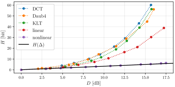
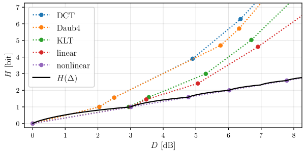
Figure 2: Empirical entropy–distortion plots for transform codes constrained to discrete cosine transform (DCT), Daubechies 4-tap wavelet (Daub4), Karhunen–Loève transform (KLT), arbitrary linear transforms, and nonlinear transforms implemented by ANNs. We also plot the entropy–distortion function of the source. The bottom panel shows the same data, zoomed in to the low-rate regime.

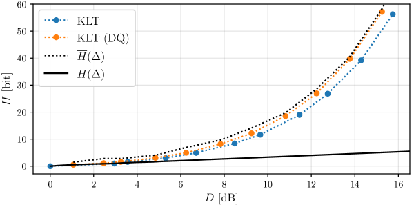
Figure 3: Empirical entropy–distortion plot for transform codes constrained to Karhunen–Loève transform (KLT) with/without dithered quantization (DQ). We also plot the entropy–distortion function of the source, and the bound developed in (58).

We compare the performance of experimentally-trained ANNs against the optimal entropy-distortion tradeoff in Eq. 22 and various linear-transform-based schemes. We follow the approach summarized by [1]. To represent the sawbridge digitally, we sample $t$ at 1024 equidistant points between 0 and 1; thus, each realization is represented as a 1024-dimensional vector. Due to this discretization, only a finite number of realizations are possible, and we took care to keep this number high enough such that none of the transform codes were able to exploit it. We optimize over three sets of model parameters: the weights and biases of an analysis ($f$) and synthesis ($g$) transform, both of which are represented by ANNs, as well as the parameters of a non-parametric entropy model $p$. Note that we do not assume that the analysis and synthesis transforms form exact inverses of each other; not only would this be difficult to enforce with ANNs, it is also not necessarily optimal. We employ ANNs of three layers, with 100 units each (except for the last), and leaky ReLU as an activation function (except for the last), for each of the transforms. We perform uniform scalar quantization of the transform coefficients, and use an entropy model that assumes independence between each of the latent dimensions; i.e., each transform coefficient is assumed to be encoded separately. The objective is to minimize the Lagrangian in Eq. 42, as in [1].

To make the comparison with linear transform coding schemes fair, we optimize linear transforms using the same methodology (linear transforms are special cases of ANNs, with just one layer). For a comparison with specified orthonormal transforms, we express the analysis transform as the composition of a fixed orthonormal matrix with a trainable diagonal scaling matrix (and analogously for the synthesis transform, in reversed order). The scaling enables uniform quantization with different effective step sizes in each latent dimension.

Empirical results are plotted in Fig. 2. Each point in the plots represents the outcome of one individual optimization of the Lagrangian in Eq. 42 with a particular predetermined value of $\lambda$, and with a predetermined constraint on the transforms (as described above). We spaced $\lambda$ logarithmically in order to cover a wide range of possible trade-offs. Both $H$ and $D$ are computed as empirical averages over $10^{7}$ source realizations, where $H$ represents the cross-entropy between the fitted entropy model $p$ and the empirical distribution of the coefficients, and $D$ is mean squared error across $t$. The top panel in the figure illustrates that the growth rate of the entropy of the linear transform codes is highly suboptimal, especially when the linear transform is further constrained to coincide with a fixed orthogonal transform such as the DCT, KLT, or a wavelet transform. In the bottom panel, we observe that the nonlinear transform code is essentially optimal. Since the transform codes are optimized for the Lagrangian, they settle into the “kinks” of the entropy–distortion function, as discussed in Section 3 (note that not all of the kinks are occupied; this is due to the pre-determined spacing of $\lambda$). As predicted by the theory, we find that a transform code with a linear analysis transform and a nonlinear synthesis transform, optimized with the same method, performs the same as the nonlinear code plotted in the figure (not shown).

Inspection of the latent-space activations as well as the entropy model reveal that linear transforms require successively larger numbers of latent dimensions as the rate increases. Nonlinear codes, on the other hand, use only a small number of latent dimensions (additional dimensions allowed for by the experimental setup are collapsed to zero-entropy distributions by the optimization procedure), implying that they successfully discover the low-dimensional structure of the source. In fact, we find that when constraining the latent space to a single dimension, the nonlinear codes do just as well. A simple explanation for why they may choose to use more dimensions in some cases is that an entropy model consisting of a single uniform distribution over a discrete set of states can be factorized into a product of multiple uniform distributions, as long as the number of states is not prime.

To illustrate the optimal KLT-constrained code from Section 4, and to verify that our optimization methodology is valid for linear codes, we plot $\overline{H}(\Delta)$ from Eq. 57 and the optimal tradeoff, $H(\Delta)$, along with empirical results for a KLT-constrained code with and without dithered quantization, in Fig. 3. Note that $\overline{H}(\Delta)$ and the curve for dithered quantization are quite close, especially at high rates.

References

- [1] Johannes Ballé et al. “Nonlinear Transform Coding” to appear In IEEE Trans. on Special Topics in Signal Proc., 2020 DOI: 10.1109/JSTSP.2020.3034501
- [2] Moshe Leshno, Vladimir Ya. Lin, Allan Pinkus and Shimon Schocken “Multilayer Feedforward Networks with a Nonpolynomial Activation Function Can Approximate Any Function” In Neural Networks 6.6, 1993 DOI: 10.1016/S0893-6080(05)80131-5
- [3] Geoffrey E. Hinton and R.. Salakhutdinov “Reducing the Dimensionality of Data with Neural Networks” In Science 313.5786, 2006 DOI: 10.1126/science.1127647
- [4] Toby Berger “Rate Distortion Theory: A Mathematical Basis for Data Compression” Englewood Cliffs, NJ: Prentice Hall, 1971
- [5] William A. and Amir Said “Digital Signal Compression: Principles and Practice” Cambridge University Press, 2011
- [6] Olivier Hénaff, Johannes Ballé, Neil C. Rabinowitz and Eero P. Simoncelli “The Local Low-Dimensionality of Natural Images” In 3rd Int. Conf. on Learning Representations (ICLR), 2015 arXiv:1412.6626
- [7] David L. Donoho, Martin Vetterli, R.. DeVore and Ingrid Daubechies “Data Compression and Harmonic Analysis” In IEEE Trans. Inf. Theory 44.6, 1998 DOI: 10.1109/18.720544
- [8] Yves Meyer “Wavelets and Applications” In Lecture at CIRM Luminy meeting, 1992
- [9] A.. Wagner and Johannes Ballé “Neural Networks Optimally Compress the Sawbridge” to appear on arXiv
- [10] Walter Rudin “Principles of Mathematical Analysis” McGraw-Hill, 1976
- [11] Gerald B. “Real Analysis” Wiley Interscience, 1999
- [12] Eugene Wong and Bruce Hajek “Stochastic Processes in Engineering Systems” New York: Springer-Verlag, 1985
- [13] Thomas M. Cover and Joy A. Thomas “Elements of Information Theory” Hoboken: John Wiley & Sons, 2006
- [14] Wojciech Szpankowski and Sergio Verdú “Minimum Expected Length of Fixed-to-Variable Lossless Compression Without Prefix Constraints” In IEEE Trans. on Inf. Theory 57.7, 2011 DOI: 10.1109/TIT.2011.2145590
- [15] András György and Tamás Linder “Optimal Entropy-Constrained Scalar Quantization of a Uniform Source” In IEEE Trans. on Inf. Theory 46.7, 2000, pp. 2704–2711 DOI: 10.1109/18.887885
- [16] Ram Zamir and Meir Feder “Rate-Distortion Performance in Coding Bandlimited Sources by Sampling and Dithered Quantization” In IEEE Trans. Inf. Theory 41.1, 1995, pp. 141–154
- [17] Ram Zamir and Meir Feder “On Universal Quantization by Randomized Uniform/Lattice Quantizers” In IEEE Trans. Inf. Theory 38.3, 1992, pp. 428–436