Pairing function of visual binary stars

Abstract

An all-sky sample of 1227 visual binaries based on Washington Double Star catalogue is constructed to infer the IMF, mass ratio, and projected distance distribution with a dedicated population synthesis model. Parallaxes from Gaia DR2 and Hipparcos are used to verify the distance distribution. The model is validated on the single-star Tycho-2 sample and successfully reproduces the observed magnitudes and angular separations. The projected separation distribution follows $f(s)\sim s^{-1.2}$ in $10^{2}-2\cdot 10^{3}$ AU range for 1–4.5 $m_{\odot}$ primary stars. Several algorithms are explored as pairing functions. Random pairing is confidently rejected. Primary-constrained (PCP) and split-core pairing (SCP), the scenarios adopting primary component’s or total system’s mass as fundamental, are considered. The preferred IMF slope is $\alpha\sim 2.8$ either way. A simple power-law mass ratio distribution is unlikely, but the introduction of a twin excess provides a favourable result. PCP with $f(q)\sim q^{-1}$ is preferred with a tiny twin fraction, models with $f(q)\sim q^{-1.5}$ are acceptable when a larger twin excess is allowed. SCP is similar to PCP when a larger slope of the power law is adopted: $f(q)\sim q^{\beta+0.7}$.

1 Introduction

Stellar mass at birth is a single parameter, which predominantly determines future evolution and observational characteristics of a star. The initial stellar mass distribution (IMF) is of crucial importance, as it encodes complex star formation process, knowledge and understanding of the IMF is essential in many areas of astronomy. It cannot be observed directly and should be estimated from indirect techniques (Kroupa et al., 2013). Universality of the stellar IMF and its dependence on the local environment remains an open issue (Bastian et al., 2010; Krumholz, 2014; Offner et al., 2014). Stellar multiplicity is closely linked to the IMF in many senses (Kroupa & Jerabkova, 2018). It can be considered as an obstacle, creating a bias for the IMF determination, but binary systems themselves imprint valuable information on the star formation and evolution history. Creating a theoretical model reproducing observational properties of the multiple star population is a challenging task yet to be solved (Goodwin et al., 2007; Lee et al., 2020).

The universality of stellar multiplicity is a subject of debate (King et al., 2012; Marks et al., 2014). Field stars represent a diverse population of various age formed in different environment. There are indications that nearby star formation regions and open star clusters are not representative of the majority of field stars (Duchêne et al., 2018; Deacon & Kraus, 2020). Binaries with orbit size $a>10^{2}$ AU are progressively affected by the dynamical destruction according to numerical simulations (Parker et al., 2009; Dorval et al., 2017), however field population remains indicative of the primordial conditions (Parker & Meyer, 2014). The ratio of the secondary companion’s mass to that of the primary, $q=m_{2}/m_{1}$, is of particular importance, Parker & Reggiani (2013) point out that the shape of mass ratio distribution $f(q)$ is largely unaffected by the dynamical evolution and directly represents the outcome of star formation. Careful interpretation and assessment of selection effects is needed (Tout, 1991). $f(q)$ can be considered as a measure of component’s coevolution, as an independent formation leads to a steep decreasing $f(q)$ distribution, while mass transfer or competitive accretion in the circumbinary disc tends to equalize masses (Moe & Di Stefano, 2017). This factor also implies that $f(q)$ depends on the orbit size as the influence of the companion is supposed to be stronger in close pairs.

The current orbit does not necessary represent conditions during the formation of the binary system. The gravitational collapse of a protostellar clump followed by the turbulent core fragmentation and subsequent rapid migration produces companions at $\sim 10^{2}-10^{4}$ AU separation (Lee et al., 2019) and is expected to be a dominant mode for the concerned visual binaries. Companion formation through gravitational instabilities in the circumstellar disc produces closer systems (Kratter & Lodato, 2016). Distinct mechanisms are responsible for the formation of wide systems. The dissolution of star clusters appears to play a major role (Kouwenhoven et al., 2010; Moeckel & Clarke, 2011) for the existence of pairs with low binding energy. Evolution of a triple system leading to the ejection of a companion into a distant orbit (Reipurth & Mikkola, 2012) and interaction of neighbouring protostellar cores (Tokovinin, 2017) are other possible mechanisms for the formation of wide binaries.

Binaries are ubiquitous and represent a broad spectrum of phenomena observed in the whole electromagnetic spectrum and beyond (Abbott et al., 2017). Detached unevolved systems are normally observed as spectroscopic, visual, common proper motion, or eclipsing binaries in optical wavelengths. Creating a large unbiased sample representing principal properties of a stellar population is challenging (Duchêne & Kraus, 2013). The available samples are often small, leading to large error margins and occasionally contradicting results in the literature. Below I list several results concerning the $f(q)$ power-law slope $\beta$ for solar-mass primaries, emphasizing the large scatter of the reported values, $q>0.2$. Metchev & Hillenbrand (2009) find $\beta\sim-0.4$, valid for 28 – 1590 AU separation. No variation of $\beta=-0.5\pm 0.29$ with separation is found according to Reggiani & Meyer (2011), $f(q)$ of M- and G-type stars appear to be consistent with A- and late B-type stars. Reggiani & Meyer (2013) later confirmed no dependence on separation, but obtained $\beta=0.25\pm 0.29$. Tokovinin & Lépine (2012) suggest that the mass ratios of wide systems ($\sim 10^{4}AU$) in the solar neighborhood are distributed nearly uniformly with a possible deficit at $q\sim 0.5$. Important characteristic of the $f(q)$ distribution is the probable increased frequency of equal-mass binaries ($q\sim 1$). Originally found for close spectroscopic systems (Lucy & Ricco, 1979), it is believed to be a common feature for a broad separation range (Söderhjelm, 2007; El-Badry et al., 2019). The origin of twin stars is being discussed (Tokovinin, 2000; Tokovinin & Moe, 2020; Adams et al., 2020).

In this paper, I attempt to infer the initial mass, mass ratio and projected separation distribution evaluating an all-sky sample of field visual binary stars with a population synthesis model. Sections 2 and 3 describe the binary-star sample and the model, its validity is tested on single-star population in Section 4. Section 5 describes the comparison of the model predictions with observational data for binary stars, and I sum up the results in Section 6.

2 Binary-star sample

2.1 Selection function

The sample of binary stars is based on the Washington Double Star Catalogue (WDS) (Mason et al., 2001), which is a principal database for visual binaries. WDS is a compilative catalogue combining diverse observational data from various sources. Indeed, some visual binaries are observed for several centuries, the historic measurements remain scientifically valuable (Mayer, 1779; Herschel & Watson, 1782; Lewis, 1893; Tenn, 2013). Such composite dataset is obviously non-homogeneous and it is essential to evaluate observational biases before proceeding for further analysis.

The principal observational parameters of visual binaries are the primary’s and secondary’s apparent magnitudes $mag_{1}$, $mag_{2}$ ($mag_{1}\leq mag_{2}$) and angular separation between components $\rho$. The probability to be included in the WDS for a given double star (the selection function) predominantly depends on these three parameters. The WDS contains both known gravitationally bound systems and mere projections – the optical pairs. Parallaxes or distances to the systems are not provided in the WDS and, in general case, may be unknown. Below I attempt to create a complete bias-free sample. The WDS is regularly updated, I use the version as of August, 2019.

The WDS contains thousands of systems with subarcsecond separation, the $\rho$ distribution reaches its peak around 0.5 arcsec. I moderately choose the lower limit as $\rho_{min}=0.8$ arcsec which reflects the resolution of the Tycho-2 (Høg et al., 2000) catalogue and is close to the capability of traditional ground-based telescopes. Closer systems, even if resolvable, may have photometry of inadequate quality, which disturbs the further analysis. The standard form of the WDS includes the first and the last available measurement of $\rho$ rounded to 0.1 arcsec. To reduce induced bias, I use the exact-value version, which provides the last value of $\rho$ without rounding.

Concerning the wide binaries, physically bound systems should be discriminated from optical pairs. Double stars with faint companions and large separation have a larger chance to be optical. It is possible to eliminate an optical pair if there is information on individual parallaxes and proper motion of the components. Another concern is a genuine physical pair with a large $\rho$ not included in the catalogue, because it is not deemed a double star by the observers, being too wide to be identified among field objects. Fortunately, there are independent datasets containing wide systems which are used to verify the completeness of the WDS. I perform cross-identification of the WDS with Andrews et al. (2017) and El-Badry et al. (2019) lists of binaries based on the Tycho-Gaia Astrometric Solution (TGAS) (Gaia Collaboration et al., 2016) and Gaia DR2 (Gaia Collaboration et al., 2018) respectively. Particularly, I search for the systems which are present in the referred Gaia-based datasets but absent from the WDS. No such binaries are found down to the limiting magnitude 9.5 and $\rho_{max}=15$ arcsec. The latter value is adopted as the maximum separation for the sample stars. Systems with $\rho\sim 1-2$ arcsec are significantly underrepresented in Gaia-based datasets due to the limitations regarding close binaries (Arenou et al., 2018). Considering that the maximum of $mag_{1}$ and $mag_{2}$ distributions for the whole WDS catalogue is between 11 and 12 mag, I expect that it is complete at least down to 9 mag for such binaries. Tycho-2 contains around 120 thousand stars brighter than 9 mag, corresponding to 2.9 stars per square degree or $5\cdot 10^{-5}$ stars per a 15 arcsec field on average. Large contamination from optical pairs is not expected; however later three pairs deemed optical were excluded thanks to Gaia DR2 data.

Another, initially unexpected, factor is related to different magnitude systems used in the WDS. Normally, infrared or any other non-visual magnitudes are marked by an appropriate code and can be easily removed. However, cross-matching with Gaia DR2 shows a significant number of stars with dramatic difference between the WDS and Gaia magnitudes, which is explained with the undeclared use of red or infrared photometry in the WDS. The number of such cases increases drastically for objects fainter than $mag=9$, giving another reason to cutoff the sample at this magnitude. The limit is applied both for the primary and the secondary component. Bright stars generally are better studied with different observational methods, there is a lower probability for them to have undiscovered companions, so I do not constrain the sample at the bright end.

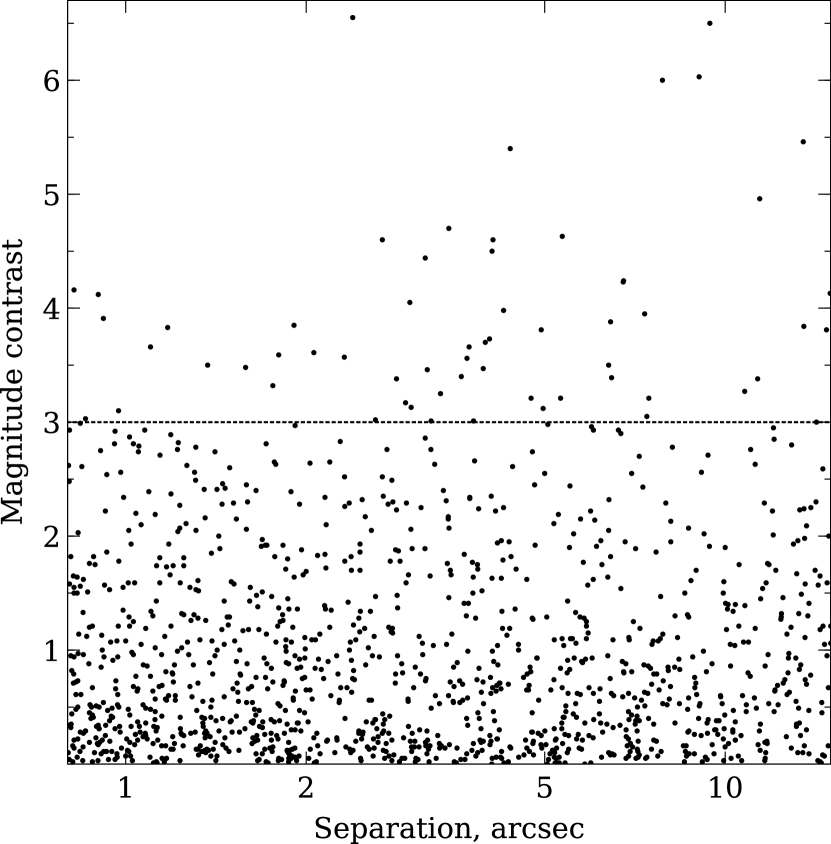
Figure 1: Observational sample binaries before cutoff of high-contrast systems, $0.8<\rho^{\prime\prime}<15~{},~{}mag_{1,2}<9$. The lack of close high-contrast pairs is clearly visible. Pairs with $\Delta mag<3$ proceed to the final sample. Sirius with $\Delta mag\sim 10$ is not shown. $\rho$ and $mag_{1,2}$ are derived from WDS, $V$ passband is expected.

One more factor for the selection function is the magnitude contrast (magnitude difference) of components, $\Delta mag=mag_{2}-mag_{1}$. Stars with similar magnitudes are more likely to be detected in comparison to binaries with high magnitude contrast. The extreme example of a high-contrast visual binary is Sirius, the brightest star in the night sky, with $\Delta mag\sim 10$ and $\rho=10.7$ arcsec. The separation – magnitude contrast diagram (Fig. 1) shows several systems with $\Delta mag\sim 5-6$, but the lack of relatively close binaries with large contrast is obvious. It seems that a close $0.8<\rho<2$ arcsec system, even if detected, would have incorrect photometry in the WDS. Considering Fig. 1, $\Delta mag<3$ is set as an appropriate limit applied for all separations. Summing up, the following conditions set up the selection function:

$$0.8^{\prime\prime}<\rho<15^{\prime\prime}~{},~{}mag_{1,2}<9~{},~{}\Delta mag<3$$ (1)

2.2 Multiple systems & excluded entries

A significant fraction of binaries are parts of multiple systems. For clarity, here I call a system multiple if it consists of three or more components. Various volume and magnitude-limited samples (Eggleton & Tokovinin, 2008; Raghavan et al., 2010; Tokovinin, 2014) show $\frac{N_{\rm Mult}}{N_{\rm Bin}+N_{\rm Mult}}\sim 20-30$ per cent fraction of multiples. In general, it may be possible to exclude known multiple systems and keep only pure binaries in the sample. I opt not to do so for two reasons. First, such approach is certainly biased, as higher-order multiplicity is characteristic for massive stars; leaving them out significantly distorts the sample. The second reason is that systems considered as binaries may have yet undiscovered companions. Therefore, I attempt to reduce multiple systems to binaries rather than exclude them. There is certainly more than one way to do it, making treatment of multiple stars one of the sources of ambiguity in the present study.

The following receipt is adopted. When the WDS contains several entries with the same designation, Eq. 1 conditions are checked. If only one pair is suitable, it proceeds to the sample alone. The most common case is that the component is a close binary on its own, for example:

WDS 00174+0853 AB, $\rho=0.162^{\prime\prime}$ , 8.38+7.78 mag

WDS 00174+0853 AB, C, $\rho=3.953^{\prime\prime}$, 7.13+7.66 mag
Here I ignore the AB pair, since its separation is less than the 0.8 arcsec limit and keep AB,C pair in the sample.

WDS 18029+5626 AB, $\rho=35.909^{\prime\prime}$, 7.78+8.14 mag

WDS 18029+5626 AC, $\rho=33.592^{\prime\prime}$, 7.78+8.53 mag

WDS 18029+5626 BC, $\rho=6.036^{\prime\prime}$, 8.14+8.53 mag

In the example shown above, all the three possible combinations for a triple system are present in the WDS. Pairs AB and AC are too wide ($\rho>15$ arcsec), so pair BC is included into the sample, while AB and AC are ignored.

Occasionally, several entries meet the criteria for component brightness and separation. Duplicate inclusion of a star in the sample is undesirable; in such cases, the pair with brighter companions is selected. In the next example, both entries meet the $\rho$ and $mag_{1,2}$ conditions, AC is chosen since its secondary companion is brighter than in the AB pair:

WDS 10441-5935 AB, $\rho=2.000^{\prime\prime}$, 8.59+8.64 mag

WDS 10441-5935 AC, $\rho=13.670^{\prime\prime}$, 7.89+8.59 mag

For several higher-order multiples (WDS 01158-6853, 05353-0523 , 05381-0011, 16120-1928, 18443+3940) it is possible to keep both AB and CD pairs, each component is included into the sample only once.

Stellar multiplicity is not limited to resolved binaries, which are contained in the WDS. Unresolved multiplicity can be suspected from spectroscopic observations or stellar variability. I do not aim for a rigorous survey of stellar multiplicity and admit that some stars in the sample are close detached, semidetached, or contact binaries. If a component of the visual binary is an unresolved or close visual binary, the WDS usually provides integral brightness of the close pair. In the particular case of equal companions, the integral brightness is 0.75 mag higher than that of an individual star. If the secondary companion is relatively faint, the difference is less significant. There are few cases when the WDS provides the resolved primary’s magnitude for a close binary instead of the integral brightness or when magnitudes for the components of a multiple system are contradictory. I choose not to alter the WDS magnitudes and treat them as is.

The WDS is primarily an astrometric catalogue, photometry is not in its prime focus, notably it lacks sources of the provided magnitudes. Cross-matching shows that, considering the sample, the absolute majority of stellar magnitudes come to the WDS from Tycho-2. Tycho-2 (Høg et al., 2000) is a dedicated homogeneous photometric catalogue, but it does not cover the sample completely, as many stars, predominantly close and faint companions, are missing. Catalog of Components of Double & Multiple stars (CCDM) (Dommanget & Nys, 2002) is another important source of magnitudes in the WDS. Photometry of visual binaries is complicated and discrepancies in different datasets are anticipated. This topic is not widely covered in the literature, I refer to Pluzhnik (2005), who have found a bias around 0.1 mag between speckle interferometry estimates and Hipparcos (Perryman et al., 1997) values. Due to the absence of a better homogeneous dataset, I stick to the WDS data.

The considered sample with $mag_{1,2}<9$ is at the bright end of Gaia DR2 (Arenou et al., 2018). Gaia data are incomplete in this magnitude range and not suited to completely replace the WDS-based sample, still it is useful for the verification of certain systems and provides parallaxes for most of them. The WDS includes some spurious systems, considering Gaia DR2 data, CCDM catalogue, and sky imagery in Aladin (Boch & Fernique, 2014), I have omitted all systems marked ‘X’ (‘Dubious Double’) and ‘K’ (infrared magnitude). Several systems with the last observation before 1991, zero number of measurements, or $mag_{2}$ unavailable in the WDS were also excluded. Additionally, the following systems were excluded due to their incorrect magnitudes:

WDS 10396-5728 is a wide pair with equally bright companions according to the WDS ($\rho=8.6$ arcsec, 8.46+8.4 mag); however 2MASS (Skrutskie et al., 2006) shows a much fainter secondary star, consistent with Gaia $G=12.2$ mag.

WDS 15365+1607 ($\rho=1$ arcsec, 8.5+8.9 mag) is not identified. Magnitudes are rounded, which is often an attribute of infrared photometry in the WDS. The coordinates refer to the high proper motion star 18 Ser of 5.9 mag, no reference on its multiplicity is found.

WDS 17404-3707 is another wide ($\rho=10.3$ arcsec) system with components of 8.3 mag according to the WDS; however, the 2MASS image clearly shows a fainter secondary companion in agreement with Gaia $G\sim 13$ mag.

The WDS 21308+4827 identifier matches two systems with almost identical $\rho$ and positional angles, but different $mag_{2}$. Gaia DR2 confirms that $mag_{2}$ is around 11 mag.

WDS 23293-8543 has $mag_{2}=10.9$ both in the CCDM and Gaia DR2, which contradicts $mag_{2}=8.53$ in the WDS.

Several other systems show magnitudes in the CCDM or Gaia DR2 slightly fainter than $mag=9$. I do not alter them on a case-by-case basis and keep the original WDS data. Additionally three pairs are removed from the sample as optical. These are WDS 17150+2450, 12095-1151, and 17150+2450, wide pairs with linear solutions according to the WDS. The Gaia DR2 parallax and proper motion data confirm that these double stars are not bound.

2.3 Distances and general sample properties

The final sample contains 1227 binaries. Gaia DR2 has a resolved $G$-magnitude photometry for both companions in 1107 cases. Distance estimates from Bailer-Jones et al. (2018) for both components are available for 1032 systems; for 155 binaries it is derived for just one companion. This leaves 40 entries without Gaia DR2 distances, inverse parallaxes $d=1/\pi$ from Hipparcos (van Leeuwen, 2007) are used for them. The only system without Gaia or Hipparcos parallax is WDS 08068-3110 (HD 67438). The B9V primary star is expected to have 0.7 mag absolute $V$ magnitude (Pecaut & Mamajek, 2013), which implies $d=363$ pc, absorption neglected. The system is located near the Galactic equator, allowing interstellar extinction around 0.5 mag, I estimate its distance around 290 pc. Thereby, beside $\rho$ and $mag_{1,2}$, distance estimates are available for all binaries in the sample. Since individual parallaxes are prone to significant errors, quartile and median values are used for comparison with the model predictions. Distance estimates for both companions provide a natural estimate of observational uncertainties.

It is important to acknowledge that Gaia algorithms treat all stars as single, whereas the sample comprises stars certainly known to be binary or multiple. However, the majority of the sample binaries have orbital periods large enough to be negligible for Gaia. A comprehensive analysis of Gaia data is beyond my scope, but it is evident that Gaia DR2 contains inaccurate or even wrong data for some of the objects. Indeed, for 138 sample binaries, the primary and secondary components’ parallaxes fall beyond their three-sigma error. There is a possibility that some of them are optical pairs, but in most cases, this discrepancy reflects Gaia systematic errors rather than actual difference in the distance. This uncertainty discourages me from creating a volume-limited sample. The furthest binary with well-agreeing components’ parallaxes is WDS 10441-5935 at $d\sim 3500$ pc. For at least 5 binaries, estimates for one of the components point out to the 4–6 kpc distance range.

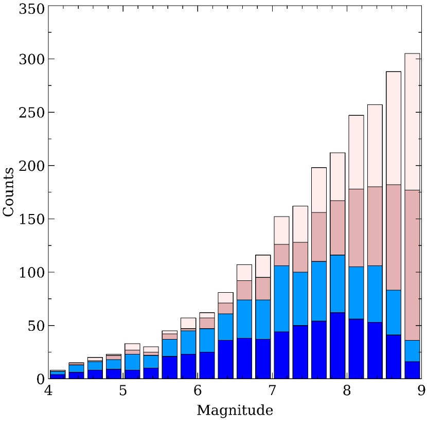
Figure 2: Apparent magnitude ($V$) distribution for the 1227 sample binaries. The areas refer to (bottom up) primaries of close ($0.8<\rho^{\prime\prime}<2.785$) and wide ($2.785<\rho^{\prime\prime}<15$) pairs, secondaries of close and wide pairs. Close and wide populations look similar.

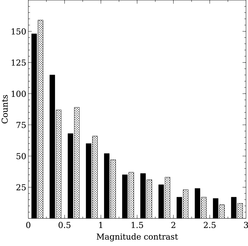
Figure 3: $V$ band magnitude contrast $mag_{2}-mag_{1}$ distribution for close (dark color) and wide sample binaries. Close pairs prevail among high-contrast systems contrary to the potential bias.

The median $\rho$ of the sample binaries is 2.78 arcsec. Fig. 2 and 3 show distributions of $mag_{1,2}$ and $\Delta mag$ for the close and wide binaries separately. No evident difference potentially caused by the observational biases or sample incompleteness is noticeable. Statistical tests show a high p-value suggesting that $mag_{1,2}$ and $\Delta mag$ are drawn from the identical distribution for close and wide binaries.

3 Population synthesis model

3.1 Overview and general assumptions

The stellar population model is based on a series of Monte Carlo experiments exercising random sampling of astrophysical parameters from prior probability distributions. Observable parameters $mag_{1}$, $mag_{2}$ and $\rho$ are calculated from astrophysical characteristics: stellar masses, ages, distances, etc. Then the selection function (Eq 1) is applied and predictions are compared to the observational sample in Section 4 and 5. I briefly explore how varying specific parameters affects the outcome in Section 4.2. This section describes general assumptions, relations, and adopted distributions of the standard model.

Although studying binaries is the main goal of the present paper, the model is used to reproduce single-star population as well, mainly for the purpose of validation. This model does not consider higher-order systems and multiplicity frequency, it creates either entirely single or binary synthetic population. Another important simplifying assumption is that stars evolve as isolated objects. Sample binaries indeed have wide orbits, the mutual influence of the components is expected to be negligible. However, if the companion is a close binary on its own, its evolution may be disturbed. Luminosity or absolute magnitude of an isolated star depends on its mass, age, and metallicity: $L=Mag_{1,2}=f(m,t,[Fe/H])$. The total number of generated objects in the model is chosen arbitrary and essentially is a compromise between computational time and convergence of the simulation results. The size of the synthetic binary sample is chosen to be at least 20 times larger than the observational dataset comprising 1227 objects.

The following underlying parameters are generated to predict observable parameters of the sample:

• Stellar mass at birth $m_{1}$ and $m_{2}$

• Stellar age $t$

• Metallicity $[Fe/H]$

• Galactic coordinates and distance $d$

• Interstellar extinction $A_{v}$

• Projected (linear) distance between components $s$

3.2 IMF and pairing functions

The distribution of primordial stellar masses is determined by the initial mass function (IMF). Power law is commonly used since pioneer research of Salpeter (1955). Popular forms of IMF used nowadays are a broken power law (Kroupa, 2001) and a combination of log-normal distribution with a power law (Chabrier, 2003). Different analytical forms exist; however, their outcomes are essentially indistinguishable (Maschberger, 2013). Therefore, I do not attempt to discriminate them and adopt a multiple-part power law. The initial stellar mass is drawn from the probability density function:

$$\dfrac{dN}{dm}\sim\begin{cases}0~{},~{}m<m_{\rm min}~{},~{}m>m_{\rm max}\\ m^{-\alpha_{1}}~{},~{}m_{\rm min}\leq m<m_{\rm split}\\ m^{-\alpha_{2}}~{},~{}m_{\rm split}\leq m\leq m_{\rm max}.\\ \end{cases}$$ (2)

Low-mass stars have low luminosities, and their contribution to the sample containing relatively bright stars is very limited. Empirically, $m_{\rm min}=0.3m_{\odot}$ is chosen as a cutoff, lower-mass stars virtually never get to the synthetic sample, but still take computational time. The selection of $m_{\rm split}$ is flexible, by default $m_{\rm split}=0.5m_{\odot}$. $m_{\rm max}=68m_{\odot}$ is determined by the availability of isochrones, but the contribution of the highest-mass stars is efficiently limited by their short lifespan anyway. Addition of a larger number of power-law segments is possible, but practically not necessary. $\alpha_{1}=1.3$ is used by default, while a wider range of $\alpha_{2}$ is explored.

IMF in Eq. 2 allows to draw a single-star population, more assumptions are needed for binaries. Various ways of pairing stars into binaries are extensively covered in Kouwenhoven et al. (2009). Different scenarios represent characteristics that are deemed to be fundamental in a particular algorithm. The four principal parameters for binaries are the primary’s and secondary’s masses $m_{1}$ and $m_{2}$, $m_{1}\geq m_{2}$, the total mass $m_{T}=m_{1}+m_{2}$, and the mass ratio $q=\frac{m_{2}}{m_{1}}~{},~{}0<q\leq 1$ . Several pairing mechanisms are considered. The most straightforward one is to assume that companions’ masses are both independently drawn from the same IMF. The star that happens to be more massive in the pair is declared primary, the other one becomes secondary, $m_{1}\geq m_{2}$. Such algorithm or pairing function is known as random pairing (RP). While RP produces very steeply decreasing $f(q)\sim q^{-\alpha_{2}}$ distribution when a restricted subset of massive stars is considered (Warner, 1961), the overall distribution is actually growing as the sample is dominated by low-mass stars (Piskunov & Malkov, 1991).

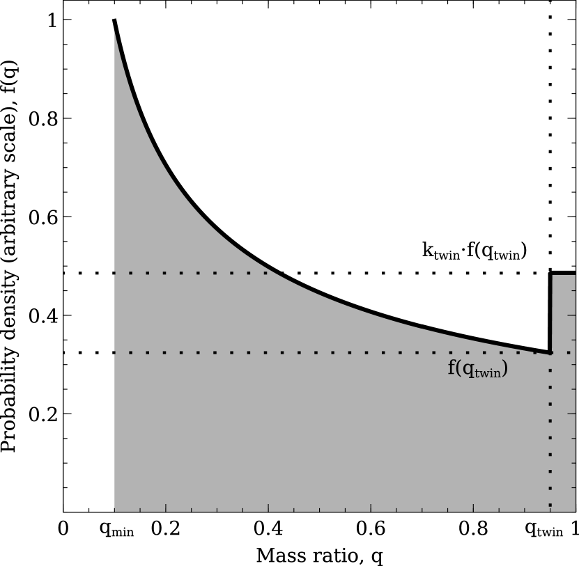
Figure 4: Mass ratio ($q=m_{2}/m_{1}$) probability density function $f(q)$ with twin excess. $q\sim q^{\beta}$ for $q_{\rm min}\leq q<q_{\rm twin}$, $q_{\rm twin}$ is always set to 0.95; in the shown example $\beta=-0.5$, $k_{\rm twin}=1.5$.

Other pairing functions imply that the components’ masses are correlated and explicitly depend on the mass ratio. Similarly to the IMF, the broken power law $f(q)=\dfrac{dN}{dq}\sim q^{\beta}$ is normally used to define the distribution, $\beta$ may vary as a function of $q$. Systems with low $q$ are unlikely to pass through the selection function (Eq. 1), making the sample not sensitive to such binaries; the use of a different $\beta$ in the low-$q$ segment is unnecessary, as the universal $\beta$ covers the whole $q$ range. There is evidence suggesting an excess of binaries with $q\sim 1$, therefore an additional twin excess is introduced to accommodate binaries with the companions of similar mass. The distribution of q in the $q_{\rm twin}\leq q\leq 1$ range is considered uniform, the probability density is multiplied by the factor $k_{\rm twin}$, see Fig. 4. The twin excess factor is derived as the ratio of one-sided $f(q)$ limits at $q=q_{\rm twin}$: $k_{\rm twin}=\dfrac{\lim_{q\to q_{\rm twin}^{+}}f(q)}{\lim_{q\to q_{\rm twin}^{-}}f(q)}$ and expresses the relative surplus of generated pairs with nearly identical companions.

$$f(q)=\dfrac{dN}{dq}\sim\begin{cases}0,~{}q<q_{\rm min}~{},~{}q>1\\ q^{\beta},~{}q_{\rm min}\leq q<q_{\rm twin}\\ 1,~{}q_{\rm twin}\leq q\leq 1,\frac{f(q_{\rm twin}+)}{f(q_{\rm twin}-)}=k_{\rm twin}\\ \end{cases}$$ (3)

$q_{\rm min}$ is set to 0.1; as already mentioned, low-$q$ systems almost never pass through the selection function; $q_{\rm twin}=0.95$, as in Moe & Di Stefano (2017). They define the twin excess as the ratio $f_{\rm twin}$ of additional twin stars with $q>0.95$ relative to the total number of binaries with $q>0.3$; this value is calculated along with $k_{\rm twin}$. $f(q)$ without the twin excess is also considered, then $f(q)\sim q^{\beta}$ for $~{}q_{\rm min}\leq q\leq 1$.

The pairing functions requiring $f(q)$ are primary-constrained pairing (PCP) and split-core pairing (SCP). PCP assumes that the primary mass $m_{1}$ is drawn from IMF; then, the $f(q)$ distribution is used to assign the mass ratio. The secondary mass is calculated as $m_{2}=q\cdot m_{1}$. Another option is SCP, which adopts IMF to draw the system’s total mass $m_{T}=m_{1}+m_{2}$ and $f(q)$ for the mass ratio. Individual masses are calculated as $m_{1}=\frac{m_{T}}{1+q}~{},~{}m_{2}=m_{T}-m_{1}$. Both for PCP and SCP, systems with $m_{2}<m_{\rm min}$ are removed. IMF (Eq. 2) is adapted for SCP, $m_{\rm min}$, $m_{\rm split}$, and $m_{\rm max}$ are multiplied by a factor of 2, as the total mass of the system is drawn, rather than that of an individual star. Goodwin (2013) noticed that SCP with flat $f(q)\sim q^{0}$ distribution was roughly similar to PCP with $f(q)\sim q^{-0.5}$. My simulations confirm the relation; however, the size of correction depends on the IMF slope, SCP with $f(q)\sim q^{\beta}$ produces a distribution almost identical to PCP with $f(q)\sim q^{\beta-0.7}$, if $\alpha_{2}=2.8$, see Fig. 5. The relation remains valid for models with the twin excess and obstructs the choice between PCP and SCP.

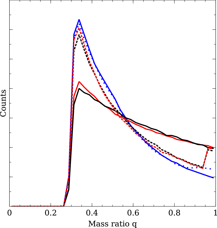
Figure 5: Produced $f(q)$ distributions for the subsample of solar-mass primaries $0.95m_{\odot}<m_{1}<1.05m_{\odot}$. $a_{2}=2.8$ is adopted for PCP and SCP. Red solid– PCP, $\beta=-0.7$; black solid– SCP, $\beta=0$; red dotted– PCP, $\beta=-1.5$, $k_{\rm twin}=1.5$; black dotted– SCP, $\beta=-0.8$, $k_{\rm twin}=1.5$; blue solid – RP, $\alpha_{2}=2$, blue dotted – RPT, $\alpha_{2}=2$, $f_{\rm twin}=0.04$. The distributions for PCP and SCP are nearly identical when $\beta$ larger by 0.7 is used for SCP. RP and RPT produce a steep $f(q)$ distribution.

Both PCP and SCP imply that $f(q)$ does not depend on stellar mass. For instance, the same f(q) is used to generate $m_{2}$ for the primary masses $m_{1}=m_{\odot}$ and $m_{1}=5m_{\odot}$. Of course, scenarios with $f(q)$ varying as a function of mass are possible and potentially may better match astrophysical processes, rather than the simple approach chosen here. The equations 2 and 3 should be considered as the generating mass and mass ratio functions. The produced distribution is different, as the systems with low-mass companions $m_{2}<m_{\rm min}$ are removed from the sample. For instance, $m_{1}=0.5m_{\odot}$ primary star happens to be generated in PCP scenario. If the drawn value of mass ratio is less than $q=\dfrac{m_{\rm min}}{m_{1}}=\dfrac{0.3m_{\odot}}{0.5m_{\odot}}=0.6$, the system would be eliminated. Hence, effectively, $f(q)=0$ for $q<0.6$ for a half-solar-mass primary. The elimination of systems with low-mass companions transforms the generated distributions, see Fig. 6 and 7. The shape of the produced functions depends heavily on $m_{\rm min}$ and $q_{\rm min}$, none the less simulations produce identical synthetic populations until $m_{\rm min}$ and $q_{\rm min}$ are small enough, reaffirming that the generating distributions determine the outcome of the model. Note that the overall $f(q)$ distribution differs significantly from the $f(q)$ produced for a specific mass. Again, I refer to Kouwenhoven et al. (2009) for a complete review of pairing scenarios.

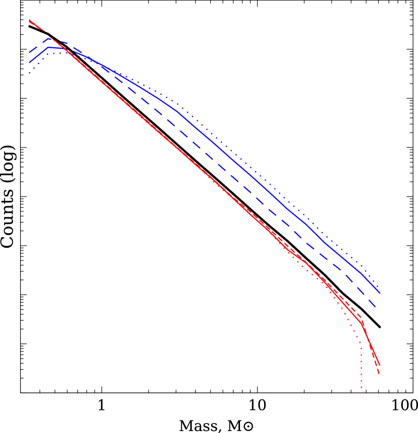
Figure 6: Generating and produced mass distribution for PCP pairing mechanism with different $f(q)$. The black solid curve is the generating IMF, $\alpha_{2}=2.8$ in Eq. 2. The dashed curve: $f(q)\sim q^{0}$; dotted curve: $f(q)\sim q^{-2}$; colored solid curve: $f(q)\sim q^{-1.5}$ with twin excess $k_{\rm twin}=1.5$. Distribution of primary components $m_{1}$ is shown in blue; red is reserved for secondary components $m_{2}$. Although the shape of the produced distribution depends heavily on $m_{\rm min}$ and $q_{\rm min}$, properties of the produced synthetic sample remain unaltered until these parameters are small enough.

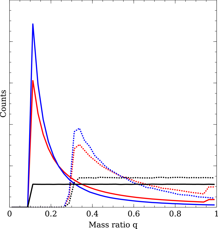
Figure 7: Generating and produced mass ratio distribution for PCP with different $f(q)$. Solid curve: generating distribution; dotted curve: produced distribution for a subsample of solar-mass primaries $0.95m_{\odot}<m_{1}<1.05m_{\odot}$. Color refers to various $f(q)$: black $\sim q^{0}$, blue $\sim q^{-2}$, red $\sim q^{-1.5}$ with twin excess $k_{\rm twin}=1.5$.

In addition to RP, PCP, and SCP, I consider distinct random pairing + twins scenario (RPT). Under this algorithm, masses $m$ are initially assigned according to the IMF, Eq. 2. Then, most stars are paired through normal random pairing. However, the small fraction of stars $f_{\rm twin}$ forms a distinct twin population. Masses of these twin stars are divided according to normal distribution $f(Q)\sim N(\mu=0.5,\sigma=0.02)$, $m_{1}=Qm$, $m_{2}=m-m_{1}$. $m_{1}$ and $m_{2}$ may be switched to ensure $m_{1}\geq m_{2}$. The resulting median $q=m_{2}/m_{1}$ for the population of twin stars is around 0.95, matching $q_{\rm twin}$ used for the PCP and SCP algorithms. Normal random pairing can be considered as RPT with $f_{\rm twin}=0$. The produced $f(q)$ distribution for RP and RPT scenarios is shown in Fig. 5.

3.3 Age and metallicity distribution

The model assumes that the stellar IMF does not change over time, stellar ages are drawn independently from masses. A constant star formation rate (SFR) is often used as a first approach; however, it is not able to reproduce accurately the Tycho-2 data and decreasing SFR is favoured (Czekaj et al., 2014). Here I adopt a simple exponential law:

$$\dfrac{dN}{dt}\sim\exp{\gamma t}$$ (4)

Considering table 7 from Aumer & Binney (2009), I set $\gamma=0.1~{}Gyr^{-1}$, $t_{\rm max}=13$ Gyr, current SFR is at 27 per cent of the initial level. The minimum age is determined by availability of stellar isochrones, $t_{\rm min}=4\cdot 10^{6}$ years.

The last parameter required to set the stellar luminosity is metallicity. It depends on the stellar age, as older population tends to have lower $[Fe/H]$ with a larger scatter (Rocha-Pinto et al., 2000). $[Fe/H]$ is adopted normally distributed with the mean and the standard deviation being a function of stellar age, see Table 1. There are indications that binary-star properties are correlated with metallicity (Moe et al., 2019), however, low-metallicity stars are scarce in the sample and their influence is limited. Age and metallicity are assumed identical for both companions since the formation of binary by a capture is rare (Clarke & Pringle, 1991).

Table 1: Parameters of normal distribution for metallicity adopted in the model, derived from fig. 13c of Haywood (2006). For details, see Section 3.3.

$\overline{Fe/H}$	$\sigma$	ages
0	0.1	t < 2 Gyr
-0.1	0.1	2 < t < 4 Gyr
-0.1	0.15	4 < t < 8.5 Gyr
-0.2	0.2	8.5 < t < 10 Gyr
-0.5	0.3	t > 10 Gyr

After stellar mass, age, and metallicity are drawn, they are converted to luminosity with a set of isochrones produced by PARSEC 1.2S (Pecaut & Mamajek, 2013; Chen et al., 2014; Tang et al., 2014; Chen et al., 2015; Marigo et al., 2017; Pastorelli et al., 2019). The Tycho-2 $V_{T}$ band is used since most sample stars have photometry in this system; for single stars, $B_{T}$ magnitude is additionally calculated. The grid of isochrones covers stellar ages in the $6.6<\rm{\log}~{}t~{}(Gyr)<10.11$ range and metallicities in the $-1.6<[Fe/H]<0.6$ interval, with the step 0.01 and 0.1 dex, respectively. The nearest available value is selected for the stellar age and metallicity, linear interpolation is used for mass. All evolutionary sections in PARSEC are included with the exception of the final post-AGB stage; degenerated stars are absent both from the sample and the model. The IMF transforms to the present-day mass function at this stage, as the stars older than their evolutionary limit are eliminated.

3.4 Spatial distribution and extinction

Next, it is necessary to constrain the spatial distribution. The Milky Way has a complex structure (Bland-Hawthorn & Gerhard, 2016), any model is an inevitably simplified representation of the real Galactic stellar population. With the focus on bright and relatively close stars, a model consisting of the thin and thick disc is chosen. The Galactic halo or bulge are not incorporated since their input is negligible. The distinction between the thin and thick disc is defined by the stellar age, stars with $t>10$ Gyr are considered to be a part of the thick disc, while younger stars are treated as a part of the thin disc. Simple exponential laws $\dfrac{dN}{dr}\sim\exp{\dfrac{-r}{L}}$ are used for the radial distribution with the scalelength $L=2500$ and $L=3500$ pc for the thin and thick disc, respectively, $r$ is a projected distance to the Galactic center. An exponential distribution is also adopted for the vertical distribution of the thick disc, $\dfrac{dN}{dz}\sim\exp{\dfrac{-z}{h}}$ with the scaleheight $h=900$ pc, $z$ is the distance to the Galactic plane. For the thin disc the logistic (sech-squared) distribution is favoured: $\dfrac{dN}{dz}\sim\operatorname{sech}^{2}\dfrac{z}{2h}$. The thin disc scaleheight $h$ of the mono-age population is expected to increase with the stellar age $t$ (Bird et al., 2013) as the stars form close to the Galactic plane and then gradually migrate further from the equator. The receipt from Schröder & Pagel (2003) is adapted with the parameters $h_{0}=35$ pc, $h_{1}=78$ pc, $v=175\cdot 10^{-9}~{}\rm{pc\cdot yr^{-1}}$, $\tau=10^{9}$ yr (see further discussion in Section 4.2):

$$h(\rm{t})=\begin{cases}\sqrt{(h_{0}^{2}+(tv)^{2}}~{},~{}t~{}\leq 0.5\cdot 10^{9}~{}\rm{yr}\\ h_{1}\sqrt{1+t/\tau}~{},~{}t~{}>0.5\cdot 10^{9}~{}\rm{yr}\end{cases}$$ (5)

The Sun is located in the Galactic plane at $r=R_{\odot}=8.5$ kpc from the Galactic center, its vertical offset is neglected. The azimuthal distribution at the galactic center $\dfrac{dN}{d\theta}$ is uniform. The distance to the stellar system is calculated in cylindrical coordinates as $d=r^{2}+R_{\odot}^{2}-2rR_{\odot}\cos{\theta}+z^{2}$. The maximum distance is set to $d_{max}=2$ kpc for practical reasons. Test simulations with $d_{max}=5$ kpc show that the fraction of binaries with $2~{}kpc<d<5$ kpc in the generated sample falls below 0.5 per cent for all reasonable parameter choices. $d_{max}=5$ kpc is used for the single-star population model. The brightest stars in the isochrones have absolute magnitudes around -10, allowing them to be observed from larger distances; however, these stars are extremely rare and their contribution is small.

The interstellar extinction $A_{v}$ is estimated using the approximation formulas 12–13 from Gontcharov (2016). The model considers absorption in the Galactic equatorial and Gould planes and it is expected to be reliable at least up to 2 kpc, thus safely covering the sample. $A_{v}$ is assumed to be equal for both companions as the starlight passes through the same interstellar medium. The apparent stellar magnitude is finally calculated as $mag_{1,2}$=$Mag_{1,2}-5+5\log d+A_{v}$. $Mag_{1,2}$ is the absolute stellar magnitude derived from the isochrones. The standard selective extinction factor $R_{v}=3.1$ is used to calculate the $B_{T}$-band magnitude for single stars, interstellar reddening caused by the excessive absorption in blue passband is estimated as $E(B-V)=\dfrac{A_{v}}{R_{v}}=\dfrac{A_{v}}{3.1}$.

3.5 Angular and projected separation

Apart from $mag_{1,2}$, angular separation $\rho$ is a principal observational parameter specific to visual binaries. The projected separation between components is a product of $\rho$ and the solar distance $d$: $s=\rho d$. Öpik (1924) examined the statistics of projected separations and showed that the variation of frequency was low when using a logarithmic scale, implying $\dfrac{dN}{ds}\sim s^{-1}$ with a proposed upper limit at 1 pc. This conclusion remains plausible, though there are indications that a steeper $dN/ds\sim s^{-\epsilon},~{}\epsilon\sim 1.5$ distribution is observed for $s>2000\sim 5000$ AU (Lépine & Bongiorno, 2007; Tokovinin & Lépine, 2012). Notably $\epsilon=1.5$ is justified theoretically as a consequence of wide binaries’ formation during dispersion of star clusters (Tian et al., 2020). Some models prefer a lognormal function (Halbwachs et al., 2017). I adopt a broken power law with the break point at $s=5000$ AU and $\epsilon=1.6$ for large separations derived from Andrews et al. (2017):

$$f(s)\sim\begin{cases}0,s<s_{\rm min},s>s_{\rm max}\\ s^{-\epsilon}&s\leq 5000\text{ AU}\\ s^{-1.6}&s>5000\text{ AU}\\ \end{cases}$$ (6)

$s_{\rm min}$ is set at 5 AU. According to the model, less than one per cent of the systems have $a<20~{}AU$; closer systems are probably not evolutionary isolated and thus cannot be covered by this model. $s_{\rm max}=d_{max}\rho_{max}=30000$ AU if $d_{max}=2$ kpc is adopted. This value is well inside the Jacobi radius (Jiang & Tremaine, 2010), as only massive and luminous pairs are observed from the large distances. If originally formed, they are largely expected to survive in the Galactic field. Less than 5 per cent of the synthetic binaries have $s>5000$ AU, the function is kept unaltered in this range, while $\epsilon$ for closer separations is varied. The model assumes that the projected distance distribution is independent from the binary mass and age. Orbital evolution after the primary star leaves the main sequence can be significant, however, the estimated mass loss does not exceed 2 per cent for 99 per cent of systems in the synthetic sample and does affect significantly very few of the sample objects.

4 Single-star model

4.1 Standard model

The validity of the stellar population model is initially tested on single stars. A comprehensive study of the single-star IMF is beyond the scope of this paper, the single-star model is used as a tool for verification of the Galaxy model. This approach assumes that general properties, such as star formation rate or spatial distribution, are identical for single and binary populations. Their dynamical properties are different (Heggie, 1975), e.g. the scaleheight potentially may vary for single and binary stars, the model calibrated on single stars is not necessarily the best choice for the binaries. Having said this precaution, no corrections are applied, single-star model parameters are used for the simulation of binaries.

A magnitude-limited sample based on Tycho-2 catalogue is used without additional modifications. Tycho-2 contains 120521 stars down to $mag=9$ in the $V_{T}$ passband and it is expected to be nearly complete in this magnitude range (Høg et al., 2000). Observational biases are anticipated, e.g. due to significant presence of unresolved and resolved binaries. Star counts $N$ predicted in the model down to magnitude limits $mag=7,8,9$ are calculated, then the ratios $N_{9}/N_{8}$ , $N_{8}/N_{7}$ are compared to the corresponding values in Tycho-2. Additionally, the null hypothesis that the distribution of $mag$ in observational and synthetic samples arises from a common function is tested with the Kolmogorov–Smirnov (KS) and Anderson–Darling (AD) two-sample statistical tests. If the obtained $p$-value is less than 0.05 for either test, the result is considered negative. When $p$ exceeds this threshold for both the AD and KS tests, the null hypothesis is not rejected and I consider the observational sample is consistent with the model prediction. The size of the synthetic sample is chosen empirically, the larger sample reduces the impact of random fluctuations but takes more computational time. For the single-star model, the synthetic sample is at least 3 times larger than the observational one.

The predicted star counts depend on the chosen IMF slope. The best agreement between the synthetic and observational samples is found when $\alpha_{2}=2.6$, see Table 2 and Fig. 8. A steep IMF overestimates the number of faint stars; instead, smaller $\alpha_{2}$ causes an excessive abundance of bright stars. Statistical tests agree with the basic $N_{9}/N_{8}$ comparison and favour $\alpha_{2}=2.6$. As the observational and model samples are large ($N\sim 10^{5}$), the discriminatory power of the tests is high, models with the adjacent values of $\alpha_{2}=2.5$ or 2.7 are statistically rejected. The IMFs with $m_{\rm split}=0.5m_{\odot},~{}m_{\odot}$ and universal Salpeter-like $\alpha$ are considered; however, the difference is barely noticeable as low-mass stars have a limited contribution to the sample. The model produces the same number of stars with $mag<9$ as in Tycho-2 when the mass density for main-sequence stars, $m>m_{\odot}$, in the 50 pc solar radius is $n=4.5\cdot 10^{-3}\dfrac{m_{\odot}}{pc^{3}}$. This value is 10 per cent less than the mid-plane mass density estimate by Bovy (2017).

Figure 8: $V_{T}$ apparent magnitude distribution in Tycho-2 (dark) compared with the model prediction for single-star population.

Table 2: Comparison of the Tycho-2 sample with the model predictions for single stars. The impact of varying $m_{\rm split}$ and $\alpha_{2}$ on the IMF (Eq. 2) is shown, other model parameters remain fixed. $\alpha_{1}=1.3$ for $m<m_{\rm split}$ when applicable. $N_{\rm mag}$ stands for star counts down to particular magnitude. The hypothesis that the magnitude distribution for the observational and synthetic samples arises from a common distribution is not rejected by the AD and KS tests only for models with $\alpha_{2}=2.6$. * stands for Tycho-2 distances, corrected for unresolved binaries. See Section 4.1 for details.

IMF ($m^{-\alpha}$)		Star counts		Distance quartiles, pc
$\alpha_{2}$	$m_{\rm split}$	$N_{9}/N_{8}$	$N_{8}/N_{7}$	25%	50%	75%
Tycho-2		2.87	2.95	157	284	448
Tycho-2*		2.87	2.95	153	275	437
2.4	$0.5m_{\odot}$	2.81	2.9	173	288	434
2.5	$0.5m_{\odot}$	2.84	2.91	169	284	426
2.6	–	2.87	2.95	165	280	418
2.6	$0.5m_{\odot}$	2.86	2.95	164	279	417
2.6	$m_{\odot}$	2.87	2.98	166	280	416
2.7	$0.5m_{\odot}$	2.90	3.00	161	277	412
2.8	$0.5m_{\odot}$	2.92	3.04	157	273	406

Gaia DR2 provides parallaxes for the majority of Tycho-2 stars and allows to compare the distance distribution in addition to the star counts. Since Gaia is strongly biased against bright stars, the cutoff at the bright end is applied, leaving 106256 stars with $7<mag<9$ in the sample. The best-neighbourhood search in the 3 arcsec radius with the additional $G<11$ mag condition to exclude wrong matches finds 104559 Gaia DR2 entries with positive parallaxes. For the 795 stars with missing Gaia data, Hipparcos parallaxes are available (van Leeuwen, 2007), thus providing distance estimate for more than 99 per cent of the sample objects. Values of 25, 50, and 75 per cent distance quartiles are compared for the model and the sample. The distance to the sample stars is estimated as an inverse parallax $d=1/\pi$; the use of Bailer-Jones et al. (2018) distances provides marginally smaller values, e.g. shifting the median distance from 284 to 282 pc. A bias caused by the presence of unresolved binaries in the catalogue is expected. In a magnitude-limited sample, such systems are observed from a larger average distance than normal single stars. A rough estimate considering a 30 per cent fraction of unresolved binaries and realistic $f(q)$ reduces the median distance by around 10 pc. The effect is probably more significant for distant stars, as massive bright stars are generally expected to have larger multiplicity frequency.

The predicted and observed distance quartiles show moderate agreement, see Table 2. In addition to the general sample, I separately consider samples near the equatorial plane and the Galactic poles, see Table 3. The model slightly underestimates the concentration of stars and distances to far-away objects near the Galactic plane. This discrepancy can be explained both by unaccounted biases in the observational data and by model limitations. The synthetic sample suggests that 18 per cent of stars in the solar neighborhood belong to the thick disc population, in agreement with the local normalisation estimate in Fuhrmann (2011). Contribution of the thick disc stars to the synthetic sample is still low at around 7 per cent, thus undermining their impact.

Table 3: Comparison of the Tycho-2 sample to the standard and modified models for single stars. All modified models use the same parameter values as in the standard model with the exception of the specified ones and $\alpha_{2}$ of the IMF (Eq. 2), which is adjusted for correct reproduction of Tycho-2 star counts. Distance quartiles are shown separately for the equatorial plane and the Galactic poles area, distances are inferred as inverse parallaxes. Closer stars are less prone to parallax-related biases and therefore larger inconsistency for 75 per cent quartile in comparison to 25 is allowed. F(%) refers to the fraction of stars in the equatorial and polar zone, $\overline{B-V}$ is the median of the $B_{T}-V_{T}$ color distribution. See the discussion of the particular models in Section 4.2.

Model	IMF	$N_{9}/N_{8}$	Equator, $|b|<5\deg$					Pole, $|b|>60\deg$
	$\alpha_{2}$		F(%)	Distance,pc			$\overline{B-V}$	F(%)	Distance, pc			$\overline{B-V}$
Tycho 2		2.87	16.4	231	403	737	0.44	7.5	112	204	350	0.95
standard	2.6	2.86	15.4	225	370	631	0.35	8.3	116	216	336	0.98
const SFR	2.9	2.86	15.3	214	348	580	0.30	7.9	113	201	319	0.69
$\gamma=0.15$	2.4	2.88	15.7	236	388	666	0.38	8.4	120	230	349	1.03
$t_{\rm max}=12$ Gyr	2.6	2.87	15.6	226	370	627	0.34	8.1	116	215	332	0.95
$[Fe/H]$=0	2.6	2.84	15.9	226	368	636	0.30	8.1	113	208	319	1.03
no thick disc	2.5	2.85	15.8	232	384	654	0.32	8.1	119	220	338	0.99
exponential	2.5	2.87	17.2	233	383	660	0.26	8.5	138	254	376	1.00
h - 30%	2.9	2.85	15.8	195	315	501	0.46	7.7	90	174	300	0.92
h + 30%	2.4	2.87	15.3	253	427	778	0.28	8.5	141	247	362	0.99
exp, $h=200$ pc	2.4	2.87	13.3	196	324	567	0.71	8.1	111	224	349	0.69
logistic, $h=120$ pc	2.3	2.86	12.1	215	359	684	0.69	7.9	112	207	316	0.65
$A_{v}$ - 30%	2.4	2.86	19.0	278	468	823	0.22	7.2	121	224	342	0.96
$A_{v}$ + 30%	2.6	2.85	13.8	205	329	547	0.40	8.9	116	218	333	1.00

The binary-star model focuses on $V_{T}$ photometry due to lacking multicolor photometry for binaries. The situation is better for single stars: for all but 82 entries, photometry in the Tycho $B_{T}$ passband is available. Distribution of the predicted and observed $B_{T}$ apparent magnitudes and $B_{T}-V_{T}$ colors is shown in Fig. 9 and 10. It shows a rather poor agreement, and statistical tests actually consider them coming from different probability density functions. The Tycho-2 color distribution is thoroughly studied and modelled in Czekaj et al. (2014). I confirm that a very steep IMF with $\alpha_{2}\sim 3$ provides a better fit for the $B-V$ distribution; however, a shorter distance scale should be used to keep star counts in agreement that drastically contradicts the Gaia distances. Therefore, I adopt a model with more conventional $\alpha_{2}=2.6$, though it poorly fits the color distribution. This value matches well with the Gaia-based study by Sollima (2019). Note that the IMF measured in the solar neighborhood is subject to observational biases increasing the observed $\alpha$ (Parravano et al., 2018).

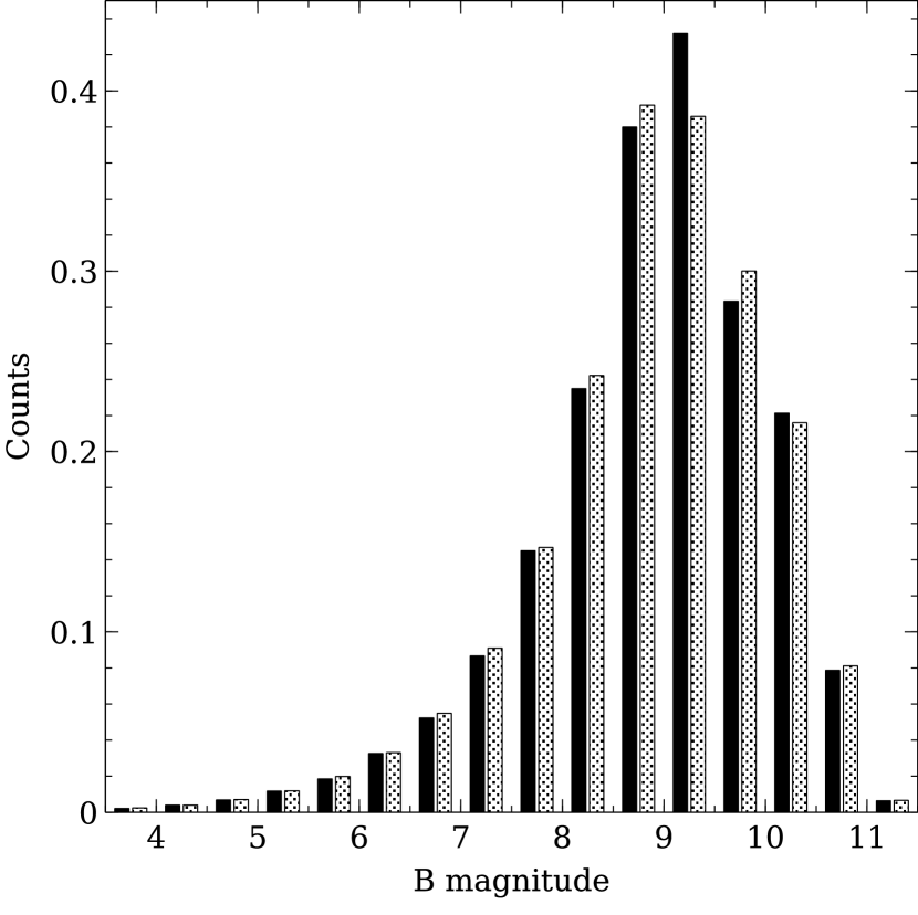
Figure 9: The $B_{T}$ apparent magnitude distribution for the restricted $V_{T}<9$ mag single-star sample (shown in dark color) compared to the model prediction.

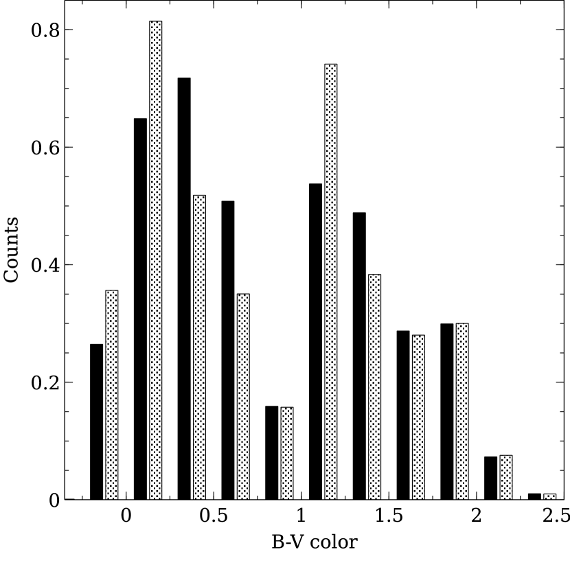
Figure 10: Comparison of the $B_{T}-V_{T}$ color distribution for single-star $V_{T}<9$ sample (dark color) to the model prediction.

4.2 Variations of the standard models

This section reviews the impact of particular parameters in the standard model presented in Table 3. When a specific parameter is changed, $\alpha_{2}$ is adjusted to ensure that the star counts and $mag$ distribution are consistent with the observational sample according to the statistical tests. IMF (Eq. 2) and SFR (Eq. 4) are strongly correlated, as the steep IMF (large $\alpha$) increases the fraction of low-mass stars in the sample, similarly to the effect of high SFR in the past. Constant SFR ($\gamma=0$) induces a steep IMF slope and a shorter distance scale in comparison to standard model parameters ($\gamma=0.1~{},~{}t_{\rm max}=13$ Gyr). Decreasing SFR (larger $\gamma$) leads to a gentle IMF slope and larger distances as old low-mass stars dominate the sample. Moderate change of $t_{\rm max}$ essentially does not affect the results. The impact of the metallicity is also limited, using the universal solar metallicity does not significantly change the outcome.

Next, I consider the impact of spatial distribution (Section 3.4). No thick disc refers to a model adopting the thin disc scaleheight law (Eq. 5) for all ages, while the standard model uses the distinct thick disc for $t>10~{}Gyr$. The difference is subtle, as the thick disc contribution is generally low. The thin disc dominates the sample and makes vertical distribution law an important part of the model. Exponential and logistic distributions were considered with various age – scaleheight dependences. In fact, none precisely reproduces the distance distribution both for the Galactic poles and equator, values in Eq. 5 are opted as the best available approximation. The original formula from Schröder & Pagel (2003) with the parameters $h_{0}=45$ pc, $h_{1}=177$ pc, $v=417~{}\rm{pc\cdot yr^{-1}}$, $\tau=10^{9}$ yr makes use of exponential distribution, however, it poorly fits the distance distribution near the Galactic poles, therefore it was adapted to the logistic distribution. A scaled decrease of $h$ leads to a steep IMF and a short distance scale, a larger value of scaleheight works in the opposite direction. Notably, the distance distribution alone can be adequately reproduced with a fixed scaleheight independent from age, but such models predict a wrong fraction of stars in the equatorial and polar zones and a wrong color distribution. The interstellar extinction law is another important factor, its adjustment significantly alters the visibility of stars near the Galactic equator.

5 Binary stars results

Here I compare the observational sample obtained in Section 2 to the model predictions discussed in Section 3. The routine is similar to the single-star model validation in Section 4, the important difference is that binaries have more observational parameters, while the observational sample is almost a hundred times smaller than that for single stars. The general sample constrained by the selection function (Eq. 1) contains $N_{9}=1227$ binaries; for $N_{8}=460$ of them, $mag_{1,2}<8$ and just for $N_{7}=168$, both components are brighter than $mag=7$. Considering that variance of the sample is a function of $\sqrt{N}$, the random error around 3 per cent is expected for the general sample and up to 8 per cent for the binaries with $mag_{1,2}<8$. A scarce sample size inevitably leads to a larger uncertainty of parameter estimates.

To minimize the effect of random fluctuations, the size of the synthetic sample is chosen at least 20 times larger than that of the observational data. The distributions of $mag_{1}$, $mag_{2}$, $\Delta mag$, and $\rho$ are compared to the corresponding model predictions using the KS and AD statistical tests; thereby, 8 separate tests are performed for each simulation, the $p$-value 0.1 is chosen as a threshold. Distance estimates are available for all sample objects, see Section 2.3. Since individual parallax values are prone to significant errors, distance quartiles are compared. Star counts (number of binaries down to a particular magnitude) and the distance distribution depend mainly on the chosen IMF slope $\alpha_{2}$, see Table 4 and 5. The value of $\alpha_{2}$ is chosen to provide consistency between the predicted and observed star counts. A steep IMF (larger $\alpha_{2}$) overproduces faint stars and induces a shorter distance scale, and vice versa.

Table 4: Outcome of random pairing + twins pairing mechanism (RPT). The $f_{\rm twin}=0$ case is standard random pairing. The $p$-value refers to the lowest one among 8 separate results of the AD and KS statistical tests for $mag_{1}$, $mag_{2}$, $\Delta mag$, and $\rho$. While this value is not reproducible due to random fluctuations during generation, it clearly represents the agreement of the model with data, the larger $p$ means better fitting. The predicted star counts meet the observational data when $\alpha_{2}=2$ is used. The reference local density $n$ for single stars is $45\cdot 10^{-4}m_{\odot}/pc^{3}$. Usually distances are available for both components of the binary, quartiles for larger and smaller estimates are shown, see Section 2.3.

scenario	IMF	Distance quartiles, pc					p-value	$N_{9}/N_{8}$	$n(M>m_{\odot})$
$f_{\rm twin}$	$\alpha_{2}$	$\overline{dist_{7}}$	$\overline{dist_{8}}$	25%	50%	75%			$10^{-4}m_{\odot}/pc^{3}$
Sample (min)		89	106	77	132	231		2.67
Sample (max)		97	109	81	139	251
0	2.0	79	105	75	138	228	0	2.7	54
0.025	2.0	85	114	81	149	248	0.06	2.68	47
0.04	1.8	98	129	95	169	276	0.21	2.58	35
0.04	2.0	90	116	82	151	252	0.49	2.66	44
0.04	2.2	77	101	71	132	225	0.15	2.79	56
0.055	2.0	94	121	85	157	261	0.11	2.64	41

Table 5: Outcomes of primary-constrained and split-core pairing (PCP and SCP) scenarios. A large set of values produces statistically acceptable results, a high $p$-value does not necessarily mean the best parameter choice. Note that the local mass density $n$ is largely dependant on the chosen twin excess $k_{\rm twin}$, while the distance distribution remains unaltered. See Fig. 14 and Section 5 for the discussion.

scenario	$\beta$	$k_{\rm twin}$	$f_{\rm twin}$	$\alpha_{2}$	$\overline{dist_{7}}$	$\overline{dist_{8}}$	25%	50%	75%	p-value	$N_{9}/N_{8}$	$n(M>m_{\odot})$
Sample (min)					89	106	77	132	231		2.67	$10^{-4}m_{\odot}/pc^{3}$
Sample (max)					97	109	81	139	251
PCP	0	1	0	2.8	89	118	82	152	250	0	2.7	15
PCP	-0.5	1	0	2.8	86	115	82	150	247	0.04	2.71	19
PCP	-1	1.1	0.01	2.6	93	122	89	160	261	0.05	2.62	22
PCP	-1	1.1	0.01	2.7	89	118	85	155	255	0.07	2.67	23
PCP	-1	1.1	0.01	2.8	86	115	82	150	246	0.18	2.67	25
PCP	-1	1.1	0.01	2.9	85	112	80	146	242	0.21	2.72	25
PCP	-1	1.1	0.01	3.0	79	106	75	140	232	0.21	2.74	27
PCP	-1.5	1.4	0.07	2.8	86	115	82	150	246	0.62	2.68	30
PCP	-2	1.8	0.17	2.6	90	120	89	159	260	0.15	2.64	41
PCP	-2	1.8	0.17	2.7	89	119	86	154	251	0.15	2.64	44
PCP	-2	1.8	0.17	2.8	84	115	84	151	247	0.15	2.66	44
PCP	-2	1.8	0.17	2.9	84	111	80	146	241	0.19	2.66	45
PCP	-2	1.8	0.17	3.0	80	109	78	142	236	0.06	2.73	48
SCP	0	1	0	2.8	88	116	84	151	245	0.02	2.68	21
SCP	0	1.1	0.01	2.8	88	117	83	153	249	0.13	2.69	20
SCP	-0.6	1.4	0.04	2.6	90	122	89	160	259	0.46	2.62	24
SCP	-0.6	1.4	0.04	2.7	87	117	84	154	251	0.51	2.65	25
SCP	-0.6	1.4	0.04	2.8	85	115	82	151	248	0.58	2.69	28
SCP	-0.6	1.4	0.04	2.9	83	113	80	146	241	0.5	2.72	29
SCP	-0.6	1.4	0.04	3.0	81	107	76	140	232	0.43	2.73	29
SCP	-1.4	2	0.16	2.8	90	117	83	151	251	0.12	2.65	41

It is noticed that the $\rho$ distribution is essentially determined by the projected distance $s$ distribution and does not depend on pairing scenarios or IMF choice. The synthetic and observed $\rho$ distributions show the best agreement when $\epsilon=1.2$ is adopted in Eq. 6, see Fig. 11. The Öpick law ($\epsilon=1$) clearly underestimates the number of close binaries, statistical tests are sharp and reject $\epsilon=1.1$ or 1.3. The angular separation is a function of the distance from the Sun, $\rho=s/d$. While a reasonable change of the model spatial distribution (Section 3.4) alters the preferred IMF slope, $\alpha_{2}$, $s$ remains largely unaffected. It is tempting to relate the deviation from $\epsilon=1$ with the effect of dynamical evolution and disruption of wide binaries. It should be kept in mind that 80 per cent of the model binaries have $90<s<2000$ AU, therefore the conclusion on preferred $\epsilon$ is valid for the limited range of separations and stellar masses, see Table 6.

Table 6: Summary of the synthetic binary-star sample population. The average of the statistically acceptable models is shown.

Parameter	10%	50%	90%
Primary mass $m_{1},m_{\odot}$	1.1	2.2	4.4
Secondary mass $m_{2},m_{\odot}$	1	1.8	3.5
Primary absolute magnitude	3.8	1	-1.1
Secondary absolute magnitude	4.6	1.9	-0.2
Mass ratio $q$	0.65	0.89	0.99
Age log $t$ (Gyr)	7.6	8.7	9.6
Metallicity, $[Fe/H]$	-0.2	0	0.1
Distance $d$, pc	45	151	372
Extinction $A_{v}$, mag	0.07	0.20	0.52
Projected separation $s$, AU	90	415	1940

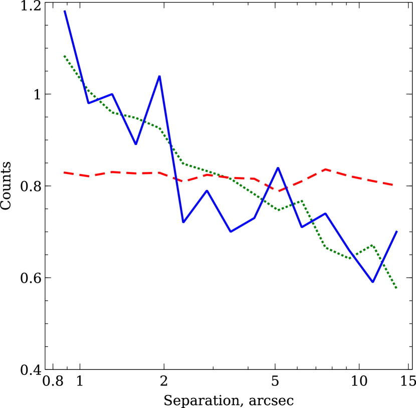
Figure 11: The distribution of angular separation ($\rho$) for the binary-star sample, the projected distance distribution slope $\epsilon$ in Eq. 6 is varied. Solid blue: observational data; red dashed: $\epsilon=1$, green dotted: $\epsilon=1.2$. The latter value is clearly favoured by the statistical tests.

Four pairing functions are examined in the paper: first, I consider random pairing (RP) and random pairing + twins scenarios (RPT), see Table 4. The star counts meet the observational data when $\alpha_{2}=2$ is adopted. However, the $\Delta mag$ distribution shows a big disagreement as the model significantly underproduces binaries with small magnitude contrast, therefore random pairing is confidently ruled out, see Fig. 12. The addition of a twin star population in the RPT algorithm improves the fit, the $p$-value of the statistical tests exceeds 0.1, and the model becomes consistent with data when the adopted fraction of twin population is $f_{\rm twin}\sim 0.03-0.055$. The distance distribution is also in a reasonable agreement, though the observational scale is slightly shorter than the model prediction. An important concern is the produced local density of binary population. The obtained mid-plane density for main-sequence single stars ($m>m_{\odot}$) is $4.5\cdot 10^{-3}\dfrac{m_{\odot}}{pc^{3}}$ (Section 4.1). The actual local density for binaries is poorly constrained, however, it certainly does not exceed the value for single stars. The inferred value for RPT is close to the single-star figure, implying that nearly all $m>m_{\odot}$ stars are binaries with a companion $m_{2}>m_{\rm min}=0.3m_{\odot}$, which seems unlikely.

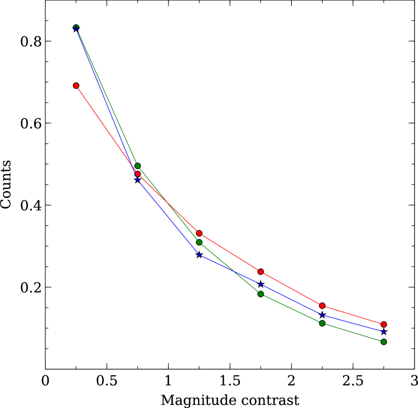
Figure 12: The magnitude contrast $\Delta mag=mag_{2}-mag_{1}$ distribution. Blue: observational sample; red: random pairing, $\alpha_{2}=2$; green: primary-constrained pairing, $\alpha_{2}=2.8$, $\beta=-0.5$, no twin excess. RP is clearly rejected due to a significant lack of binaries with equally bright companions in comparison with the observational data. PCP without twin excess fits the data better, however, the $p$-value $\sim 0.04$ is still below the threshold.

Next, I proceed to primary-constrained pairing (PCP) and split-core pairing (SCP). Both scenarios require IMF and f(q) (Eq. 2 and 3) to be assigned. Models with a fixed IMF but different $f(q)$ produce identical distance distributions and star counts (Table 5). Varying the IMF slope with a fixed $f(q)$ distribution, I favour $\alpha_{2}=2.8$ and perform further calculations for this value. Due to the small sample size, the statistical tests tolerate at least $\Delta\alpha_{2}=0.2$ error. The obtained value of IMF slope is notably different from the RPT scenario, which favours $\alpha_{2}=2$. The secondary companion mass distribution appears to be critical for the observability of a binary system in the model (Fig. 13). The $m_{2}$ distribution for RPT with $\alpha_{2}=2$ is similar to PCP and SCP with $\alpha_{2}=2.8$, matching the difference of the preferred IMF slope.

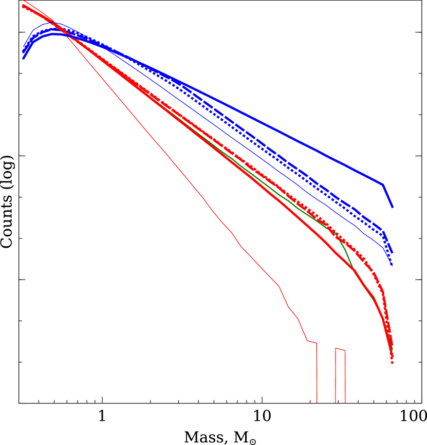
Figure 13: The produced IMF for primary (shown in blue) and secondary (red) components for several pairing mechanisms. Solid line: RP; thick: $\alpha_{2}=2$, thin: $\alpha_{2}=2.8$; dashed: PCP, $\beta=-1.5$, $k_{\rm twin}=1.5$; dotted: SCP, $\beta=-0.5$, $k_{\rm twin}=1.3$. Green: the secondary companion in RPT, $\alpha_{2}=2$, $f_{\rm twin}=0.04$, the primary overlaps the normal RP, shown in thick solid blue. The secondary companion mass distribution for RPT with $\alpha_{2}=2$ resembles PCP and SCP with $\alpha_{2}=2.8$ and determines the choice of the IMF slope.

Initially, models with a simple power slope without twin excess are tested. The best agreement is found with f(q) slope $\beta=-0.5-0.6$ in the case of PCP, but the obtained $p$-value for the $\Delta mag$ distribution is slightly below 0.05, and these models are statistically unlikely. Fig. 12 shows that the observed peak in the magnitude contrast distribution is sharper than the predicted one. The distributions for $mag_{1}$, $mag_{2}$ and $\rho$, at the same time, show a high $p$-value, emphasizing that the rejection of the model is caused by poor fitting of $\Delta mag$. Introduction of a small twin excess in $f(q)$ law improves the fit, model prediction and observational data no longer diverge statistically. A choice of a sole best-fitting combination of the mass-ratio slope and twin excess is hardly justified, as the statistical tests favour a reasonably wide set of parameters. Pairs of $\beta$ and $k_{\rm twin}$ providing an acceptable $p$-value larger than 0.1 are shown in Fig. 14 and form two parallel bands for PCP and SCP. Models with a modest mass-ratio distribution slope $\beta$ and small twin excess $k_{\rm twin}$ are acceptable along with those having rapidly decreasing $f(q)$ with a large $k_{\rm twin}$. Results for PCP and SCP are strongly correlated, as expected, reflecting the connection discussed in Section 3.2 and Fig. 5. While uniform $f(q)$ ($\beta=0$) is confidently rejected for the PCP scenario, it remains plausible for SCP with the addition of a small twin excess, though it does not stand out among other viable options.

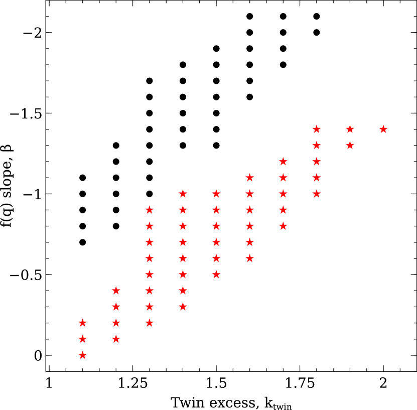
Figure 14: Values of mass-ratio distribution slope and twin excess in Eq. 3, providing successful agreement ($p$-value > 0.1 in the AD and KS tests) of the observed and synthetic $mag_{1}$, $mag_{2}$ $\Delta mag$, $\rho$ distributions for the PCP (black) and SCP (red) pairing scenarios. A choice of a sole best-fitted model appears to be unjustified. Models with large $k_{\rm twin}$ require high binary frequency and local mass density, the latter parameter is poorly constrained.

The model comprises a purely binary population and does not involve assumptions on the binary frequency. In Section 4.1, the local stellar density $n$ for $m>m_{\odot}$ stars is used to validate the single-star model. The produced $n$ for binaries potentially allows to discriminate statistically consistent models. Indeed, $n$ depends on the $f(q)$ slope: while PCP models with $\beta=-0.5$ imply $n\sim 2\cdot 10^{-3}\dfrac{m_{\odot}}{pc^{3}}$, or around 45 per cent of the single-star density, models with $\beta=-2$ require ubiquitous binary frequency, see Table 5. The reported $n$ refers to the local density of primary stars; inclusion of secondary stars with $m_{2}>m_{\odot}$ increases $n$ by approximately 15 per cent. $n$ is estimated in assumption of universal $\beta$ for the $0.1<q<0.95$ range; at the same time, the model is not sensitive to systems with low and medium mass ratios $q<0.6$, as they contribute less than 5 per cent of the objects. If $f(q)$ flattens in the low-$q$ range, which is plausible according to Moe & Di Stefano (2017), $n$ decreases and nearly 100 per cent binary frequency is no longer required. It is widely accepted that the binary frequency increases with stellar mass from roughly 0.5 for $m_{1}=m_{\odot}$ to 1 for the most massive stars, thus favouring large $n$. At the same time, the model does not cover the whole binary population, excluding close binaries with $s<5$ AU, wide $s>30000$ AU pairs, and systems with low-mass companions $m_{2}<0.3m_{\odot}$. The mentioned factors obstruct the choice of the reference $n$; however it is evident that scenarios requiring $n>4\cdot 10^{-3}m_{\odot}$ are not plausible.

The binary-star sample is constrained by the selection function, Eq. 1. While it is hard to choose the sole combination of parameters among wide range of options, statistically acceptable models produce stellar populations with similar properties, shown in Table 6. For example, the median primary mass of the population is $2.2m_{\odot}$, just for 10 per cent of the objects $m_{1}<1.1m_{\odot}$ or $m_{1}>4.4m_{\odot}$. Efficiently, the conclusions on pairing mechanisms and underlying distributions are valid for a limited range of parameters. I find particularly instructive that, while the synthetic sample with median $q=0.89$ is dominated by the stars with large $q$, the high fraction of twins in the overall population is not necessary to explain the observed distribution.

Finally, I compare the results with those available in the literature. Moe & Di Stefano (2017) compiled various sets of observations, including Shatsky & Tokovinin (2002), Raghavan et al. (2010) and De Rosa et al. (2014), to provide estimates of $\beta$ and $f_{\rm twin}$ separately for different ranges of masses and orbital periods. My calculations are made in terms of projected distance $s$, the exact relation of $s$ and semi-major axis $a$ depends on the distribution of orbital elements, including eccentricity and inclination. For this purpose, it is enough to assume that the projected semi-major axis $a$ is 10–20 per cent larger than $s$ (Couteau, 1960; Heintz, 1969). Applying Kepler’s third law of motion $P\sim\sqrt{\frac{a^{3}}{m}}$, I estimate that the majority of sample-star periods fall into 5 < log $P$ (days) < 7 category. According to Moe & Di Stefano (2017), $f(q)$ slope is drastically steeper for massive binaries and larger periods, the presence of a twin-star population is noticeable only for close and lower-mass binaries, see Table 7. However, the considered samples are small and the assessment of the respective observational biases is challenging. My model adopts universal $f(q)$ regardless of the orbital period, huge variance of $\beta$ for the adjacent parameter domains in the referenced paper is alarming and makes comparison ill-conditioned. Marginalising Moe & Di Stefano (2017) results, small $f_{\rm twin}$ with $\beta\sim-1.5$ can be expected, though the uncertainty of $f(q)$ slope is high. My model predicts $f(q)$ with a modest slope $\beta\sim-1$ with a low $f_{\rm twin}$. A steeper $f(q)$ slope is also possible, but requires a larger twin fraction.

Table 7: Excerpt of table 13 from Moe & Di Stefano (2017) and table G1 from El-Badry et al. (2019) covering the modelled range of primary masses, orbital periods (log $P$, days), or separations $s$ (AU) compared to the outcome of the PCP pairing mechanism. Three hypotheses on the fraction of twin stars are shown.

$m_{1}$, $m_{\odot}$	log $P$ or $s$	$\beta$	$f_{\rm twin}$
	log $P~{}=~{}5$	$-0.5\pm 0.3$	$0.10\pm 0.03$
	$50<s<350$	$-1.2\pm 0.7$	$0.1\pm 0.03$
0.8 — 1.2	$350<s<600$	$-1.8\pm 0.4$	$0.05\pm 0.02$
	$600<s<1000$	$-1.4\pm 0.3$	$0.04\pm 0.02$
	$1000<s<2500$	$-1.5\pm 0.2$	$0.01\pm 0.01$
	log $P~{}=~{}7$	$-1.1\pm 0.3$	$<0.03$
	$50<s<350$	$-0.9\pm 1.0$	$0.09\pm 0.08$
1.2—2.5	$350<s<600$	$-1.9\pm 0.5$	$0.09\pm 0.05$
	$600<s<1000$	$-1.2\pm 0.3$	$0.02\pm 0.03$
	$1000<s<2500$	$-1.6\pm 0.2$	$0.00\pm 0.02$
2—5	log $P~{}=~{}5$	$-1.4\pm 0.3$	$<0.03$
2—5	log $P~{}=~{}7$	$-2.0\pm 0.3$	$<0.03$
PCP, small twin fraction		$-0.9\pm 0.2$	0.01
PCP, medium twin fraction		$-1.5\pm 0.2$	0.07
PCP, large twin fraction		$-2.0\pm 0.1$	0.17

The results are also compared to the El-Badry et al. (2019) study, based on Gaia DR2 data, which provides a detailed coverage of the $f(q)$ dependence on projected separation. For solar-mass primaries, El-Badry et al. (2019) clearly expect a steeper $f(q)$ than Moe & Di Stefano (2017), see Table 7. No clear trend for $\beta$ as a function of $s$ is seen, error margins are significant. Notably, $\beta=-1.5$ is within one-sigma error for all considered data domains, this fact probably justifies the use of universal $\beta$ in my model. A twin excess is noticeable for less massive and, as expected, closer binaries. El-Badry et al. (2019) sample misses $m_{1}>2.5_{\odot}$ stars, Moe & Di Stefano (2017) show that the $f(q)$ slope is steeper for massive primaries, while $f_{\rm twin}$ is lower. Propagating this trend to the missing domain in El-Badry et al. (2019) leads to efficient $\beta\sim-1.5$ with small to moderate $f_{\rm twin}$.

6 Conclusions

After reviewing observational biases and adopting the selection function (Eq. 1), an all-sky sample of 1227 visual binaries is created based on the WDS catalogue and supplied with parallaxes from Gaia DR2 and Hipparcos in Section 2. A population synthesis model adopts various hypotheses about pairing mechanisms and fundamental parameter distributions to transform them into apparent magnitudes and angular separations in Section 3. The produced distributions are tested against actual data using the Kolmogorov – Smirnov and Anderson – Darling statistical tests. In Section 4, the model is calibrated on single stars, favouring the single-star IMF slope $\alpha_{2}=2.6$ (Eq. 2), though this value depends on the adopted SFR (Eq. 4), see Table 2 and 3.

The main simulation results for binary stars are presented in Section 5. It is noticed that the projected distance distribution is largely independent of the assumptions on IMF, $\epsilon=1.2$ is favoured in Eq. 6. Then, four pairing functions are considered. Random pairing is confidently rejected (Fig. 12), as it significantly underproduces binaries with low magnitude contrast. A mix of random pairing with a distinct twin population is statistically consistent when $\alpha_{2}=2\pm 0.2$ and $f_{\rm twin}\sim 0.04\pm 0.015$, but implies the entire population to be binary, which is presumed unlikely, see Table 4.

Next, primary-constrained and split-core pairing (PCP and SCP) with the universal power law $f(q)$ are considered. They provide a better agreement, but the produced $\Delta mag$ distribution is still statistically rejected. However, introduction of a small twin excess creates favourable models (Table 5). The inferred IMF slope for PCP and SCP $\alpha_{2}=2.8\pm 0.2$ does not depend on the $f(q)$ choice. Combinations of acceptable mass-ratio function slope $\beta$ and twin excess $k_{\rm twin}$ (Eq. 3) are shown in Figure 14 and represent two parallel bands. SCP, which assumes the total system’s mass to be fundamental, requires $\beta$ larger by $\sim 0.7$ in comparison to PCP. PCP considers the primary mass as a principal parameter and favours $\beta\sim-1$, if the twin fraction $f_{\rm twin}$ is as small as 0.01. A larger twin excess is possible and induces a steeper $f(q)\sim q^{-1.5}$ distribution with a higher binary frequency. The latter factor makes scenarios with large $f_{\rm twin}$ improbable.

The model successfully reproduces the observed $mag_{1,2}$, $\Delta mag$, and $\rho$ distributions according to statistical tests, distance estimates inferred from parallaxes are also in a moderate agreement. The limits of the model reliability are efficiently constrained by the observational sample. Although a large grid of parameters is used in the input, characteristics of most stars passed to the final synthetic sample lie in a fairly bound parameter space. General properties of the synthetic population are nearly invariant for all statistically acceptable models, see Table 6. 80 per cent of the primary masses are in the $\sim$ 1 — 4.5 $m_{\odot}$ interval, the projected separation lies in the $\sim 10^{2}-2\cdot 10^{3}$ AU range. Only 10 per cent of systems have $q<0.65$. These values highlight limitations of the model, conclusions on the pairing function, IMF, $f(q)$, and $f(s)$ are valid for a specified range of stellar masses and separations, as sensitivity of the model is low outside it.

The results are relatively in line with the recent Moe & Di Stefano (2017) and El-Badry et al. (2019) papers, though the obtained $f(q)$ slope is more modest, see Table 7. Contrary to this study, the referred papers allow and report $f(q)$ depending on the projected distance or orbital period. My model adopts a universal $f(q)$ and still successfully reproduces the observed distributions. This fact does not mean that stellar masses and separations are independent, but implies that such approximation works fairly well for the concerned parameter space. Caution is needed, as the authors use slightly different parametrization for the twin excess. Unlike the studies referred to, the present sample is obtained without use of a parallax cutoff or Gaia’s photometric data, thus avoiding the risk of related systematic biases.

Finally, it should be acknowledged that the described population synthesis model involves a number of simplifying assumptions, both at the stage of sample assessment and numerical simulations. Some of them are disputable, if not wrong. Those include treatment of multiple stars, contact and semidetached components, while the evolutionary model considers isolated stars. Photometry quality for the sample is questionable, a dedicated multicolor survey is crucial for a proper further analysis. The chosen pairing mechanisms are basic and do not depend on stellar mass, age, or orbit size. They successfully reproduce the fairly small observational sample, but it is probable that a larger multicolor dataset will require a more sophisticated approach.

Data availability

The data and code underlying this article are available in the GitHub Repository at https://github.com/chulkovd/synthesis.

References

- Abbott et al. (2017) Abbott B. P., Abbott R., Abbott T. D., Acernese F., Ackley K., Adams C., 2017, ApJ, 848, L12
- Adams et al. (2020) Adams F. C., Batygin K., Bloch A. M., 2020, MNRAS, 494, 2289
- Andrews et al. (2017) Andrews J. J., Chanamé J., Agüeros M. A., 2017, MNRAS, 472, 675
- Arenou et al. (2018) Arenou F., et al., 2018, A&A, 616, A17
- Aumer & Binney (2009) Aumer M., Binney J. J., 2009, MNRAS, 397, 1286
- Bailer-Jones et al. (2018) Bailer-Jones C. A. L., Rybizki J., Fouesneau M., Mantelet G., Andrae R., 2018, AJ, 156, 58
- Bastian et al. (2010) Bastian N., Covey K. R., Meyer M. R., 2010, ARA&A, 48, 339
- Bird et al. (2013) Bird J. C., Kazantzidis S., Weinberg D. H., Guedes J., Callegari S., Mayer L., Madau P., 2013, ApJ, 773, 43
- Bland-Hawthorn & Gerhard (2016) Bland-Hawthorn J., Gerhard O., 2016, ARA&A, 54, 529
- Boch & Fernique (2014) Boch T., Fernique P., 2014, in Manset N., Forshay P., eds, Astronomical Society of the Pacific Conference Series Vol. 485, Astronomical Data Analysis Software and Systems XXIII. p. 277
- Bovy (2017) Bovy J., 2017, MNRAS, 470, 1360
- Chabrier (2003) Chabrier G., 2003, PASP, 115, 763
- Chen et al. (2014) Chen Y., Girardi L., Bressan A., Marigo P., Barbieri M., Kong X., 2014, MNRAS, 444, 2525
- Chen et al. (2015) Chen Y., Bressan A., Girardi L., Marigo P., Kong X., Lanza A., 2015, MNRAS, 452, 1068
- Clarke & Pringle (1991) Clarke C. J., Pringle J. E., 1991, MNRAS, 249, 584
- Couteau (1960) Couteau P., 1960, Journal des Observateurs, 43, 41
- Czekaj et al. (2014) Czekaj M. A., Robin A. C., Figueras F., Luri X., Haywood M., 2014, A&A, 564, A102
- De Rosa et al. (2014) De Rosa R. J., et al., 2014, MNRAS, 437, 1216
- Deacon & Kraus (2020) Deacon N. R., Kraus A. L., 2020, MNRAS, 496, 5176
- Dommanget & Nys (2002) Dommanget J., Nys O., 2002, VizieR Online Data Catalog, p. I/274
- Dorval et al. (2017) Dorval J., Boily C. M., Moraux E., Roos O., 2017, MNRAS, 465, 2198
- Duchêne & Kraus (2013) Duchêne G., Kraus A., 2013, ARA&A, 51, 269
- Duchêne et al. (2018) Duchêne G., Lacour S., Moraux E., Goodwin S., Bouvier J., 2018, MNRAS, 478, 1825
- Eggleton & Tokovinin (2008) Eggleton P. P., Tokovinin A. A., 2008, MNRAS, 389, 869
- El-Badry et al. (2019) El-Badry K., Rix H.-W., Tian H., Duchêne G., Moe M., 2019, MNRAS, 489, 5822
- Fuhrmann (2011) Fuhrmann K., 2011, MNRAS, 414, 2893
- Gaia Collaboration et al. (2016) Gaia Collaboration et al., 2016, A&A, 595, A2
- Gaia Collaboration et al. (2018) Gaia Collaboration et al., 2018, A&A, 616, A1
- Gontcharov (2016) Gontcharov G. A., 2016, Astrophysics, 59, 548
- Goodwin (2013) Goodwin S. P., 2013, MNRAS, 430, L6
- Goodwin et al. (2007) Goodwin S. P., Kroupa P., Goodman A., Burkert A., 2007, in Reipurth B., Jewitt D., Keil K., eds, Protostars and Planets V. p. 133 (arXiv:astro-ph/0603233)
- Halbwachs et al. (2017) Halbwachs J. L., Mayor M., Udry S., 2017, MNRAS, 464, 4966
- Haywood (2006) Haywood M., 2006, MNRAS, 371, 1760
- Heggie (1975) Heggie D. C., 1975, MNRAS, 173, 729
- Heintz (1969) Heintz W. D., 1969, J. R. Astron. Soc. Canada, 63, 275
- Herschel & Watson (1782) Herschel M., Watson D., 1782, Philosophical Transactions of the Royal Society of London Series I, 72, 112
- Høg et al. (2000) Høg E., et al., 2000, A&A, 355, L27
- Jiang & Tremaine (2010) Jiang Y.-F., Tremaine S., 2010, MNRAS, 401, 977
- King et al. (2012) King R. R., Goodwin S. P., Parker R. J., Patience J., 2012, MNRAS, 427, 2636
- Kouwenhoven et al. (2009) Kouwenhoven M. B. N., Brown A. G. A., Goodwin S. P., Portegies Zwart S. F., Kaper L., 2009, A&A, 493, 979
- Kouwenhoven et al. (2010) Kouwenhoven M. B. N., Goodwin S. P., Parker R. J., Davies M. B., Malmberg D., Kroupa P., 2010, MNRAS, 404, 1835
- Kratter & Lodato (2016) Kratter K., Lodato G., 2016, ARA&A, 54, 271
- Kroupa (2001) Kroupa P., 2001, MNRAS, 322, 231
- Kroupa & Jerabkova (2018) Kroupa P., Jerabkova T., 2018, arXiv e-prints, p. arXiv:1806.10605
- Kroupa et al. (2013) Kroupa P., Weidner C., Pflamm-Altenburg J., Thies I., Dabringhausen J., Marks M., Maschberger T., 2013, The Stellar and Sub-Stellar Initial Mass Function of Simple and Composite Populations. p. 115, doi:10.1007/978-94-007-5612-0_4
- Krumholz (2014) Krumholz M. R., 2014, Phys. Rep., 539, 49
- Lee et al. (2019) Lee A. T., Offner S. S. R., Kratter K. M., Smullen R. A., Li P. S., 2019, ApJ, 887, 232
- Lee et al. (2020) Lee Y.-N., Offner S. S. R., Hennebelle P., André P., Zinnecker H., Ballesteros-Paredes J., Inutsuka S.-i., Kruijssen J. M. D., 2020, Space Sci. Rev., 216, 70
- Lépine & Bongiorno (2007) Lépine S., Bongiorno B., 2007, AJ, 133, 889
- Lewis (1893) Lewis T., 1893, The Observatory, 16, 279
- Lucy & Ricco (1979) Lucy L. B., Ricco E., 1979, AJ, 84, 401
- Marigo et al. (2017) Marigo P., et al., 2017, ApJ, 835, 77
- Marks et al. (2014) Marks M., Leigh N., Giersz M., Pfalzner S., Pflamm-Altenburg J., Oh S., 2014, MNRAS, 441, 3503
- Maschberger (2013) Maschberger T., 2013, MNRAS, 429, 1725
- Mason et al. (2001) Mason B. D., Wycoff G. L., Hartkopf W. I., Douglass G. G., Worley C. E., 2001, AJ, 122, 3466
- Mayer (1779) Mayer C., 1779, De novis in coelo sidereo phaenomenis in miris stellarum fixarum comitibus Mannhemii in specula nova elect. recens detectis. Typographia Elector. Aulica & Academica
- Metchev & Hillenbrand (2009) Metchev S. A., Hillenbrand L. A., 2009, ApJS, 181, 62
- Moe & Di Stefano (2017) Moe M., Di Stefano R., 2017, ApJS, 230, 15
- Moe et al. (2019) Moe M., Kratter K. M., Badenes C., 2019, ApJ, 875, 61
- Moeckel & Clarke (2011) Moeckel N., Clarke C. J., 2011, MNRAS, 415, 1179
- Offner et al. (2014) Offner S. S. R., Clark P. C., Hennebelle P., Bastian N., Bate M. R., Hopkins P. F., Moraux E., Whitworth A. P., 2014, in Beuther H., Klessen R. S., Dullemond C. P., Henning T., eds, Protostars and Planets VI. p. 53 (arXiv:1312.5326), doi:10.2458/azu_uapress_9780816531240-ch003
- Öpik (1924) Öpik E., 1924, Publications of the Tartu Astrofizica Observatory, 25, 1
- Parker & Meyer (2014) Parker R. J., Meyer M. R., 2014, MNRAS, 442, 3722
- Parker & Reggiani (2013) Parker R. J., Reggiani M. M., 2013, MNRAS, 432, 2378
- Parker et al. (2009) Parker R. J., Goodwin S. P., Kroupa P., Kouwenhoven M. B. N., 2009, MNRAS, 397, 1577
- Parravano et al. (2018) Parravano A., Hollenbach D., McKee C. F., 2018, MNRAS, 480, 2449
- Pastorelli et al. (2019) Pastorelli G., et al., 2019, MNRAS, 485, 5666
- Pecaut & Mamajek (2013) Pecaut M. J., Mamajek E. E., 2013, ApJS, 208, 9
- Perryman et al. (1997) Perryman M. A. C., et al., 1997, A&A, 500, 501
- Piskunov & Malkov (1991) Piskunov A. E., Malkov O. I., 1991, A&A, 247, 87
- Pluzhnik (2005) Pluzhnik E. A., 2005, A&A, 431, 587
- Raghavan et al. (2010) Raghavan D., et al., 2010, ApJS, 190, 1
- Reggiani & Meyer (2011) Reggiani M. M., Meyer M. R., 2011, ApJ, 738, 60
- Reggiani & Meyer (2013) Reggiani M., Meyer M. R., 2013, A&A, 553, A124
- Reipurth & Mikkola (2012) Reipurth B., Mikkola S., 2012, Nature, 492, 221
- Rocha-Pinto et al. (2000) Rocha-Pinto H. J., Maciel W. J., Scalo J., Flynn C., 2000, A&A, 358, 850
- Salpeter (1955) Salpeter E. E., 1955, ApJ, 121, 161
- Schröder & Pagel (2003) Schröder K. P., Pagel B. E. J., 2003, MNRAS, 343, 1231
- Shatsky & Tokovinin (2002) Shatsky N., Tokovinin A., 2002, A&A, 382, 92
- Skrutskie et al. (2006) Skrutskie M. F., et al., 2006, AJ, 131, 1163
- Söderhjelm (2007) Söderhjelm S., 2007, A&A, 463, 683
- Sollima (2019) Sollima A., 2019, MNRAS, 489, 2377
- Tang et al. (2014) Tang J., Bressan A., Rosenfield P., Slemer A., Marigo P., Girardi L., Bianchi L., 2014, MNRAS, 445, 4287
- Taylor (2005) Taylor M. B., 2005, in Shopbell P., Britton M., Ebert R., eds, Astronomical Society of the Pacific Conference Series Vol. 347, Astronomical Data Analysis Software and Systems XIV. p. 29
- Tenn (2013) Tenn J. S., 2013, Journal of Astronomical History and Heritage, 16, 81
- Tian et al. (2020) Tian H.-J., El-Badry K., Rix H.-W., Gould A., 2020, ApJS, 246, 4
- Tokovinin (2000) Tokovinin A. A., 2000, A&A, 360, 997
- Tokovinin (2014) Tokovinin A., 2014, AJ, 147, 87
- Tokovinin (2017) Tokovinin A., 2017, MNRAS, 468, 3461
- Tokovinin & Lépine (2012) Tokovinin A., Lépine S., 2012, AJ, 144, 102
- Tokovinin & Moe (2020) Tokovinin A., Moe M., 2020, MNRAS, 491, 5158
- Tout (1991) Tout C. A., 1991, MNRAS, 250, 701
- Warner (1961) Warner B., 1961, PASP, 73, 439
- Wenger et al. (2000) Wenger M., et al., 2000, A&AS, 143, 9
- van Leeuwen (2007) van Leeuwen F., 2007, A&A, 474, 653