Modeling the Current Modulation of Bundled DNA Structures in Nanopores

Abstract

We investigate the salt-dependent current modulation of bundled DNA nanostructures in a nanopore. To this end, we developed four simulation models for a 2x2 origami structure with increasing level of detail ranging from the mean-field level to an all-atom representation of the DNA structure. We observe a consistent pore conductivity as a function of salt concentration for all four models. However, a comparison of our data to recent experimental investigations on similar systems displays significant deviations. We discuss possible reasons for the discrepancies and propose extensions to our models for future investigations.

I Introduction

The field of nanopore based molecule detection and analysis has shown growing interest in the soft matter scientific community in the last years. The basic idea dates back to the late 1940s when Wallace Coulter Coulter (1953) invented a device to count red blood cells in a setup consisting of two electrolyte reservoirs in an electric field. A small orifice connecting the two reservoirs lead to a finite conductivity. For the pure salt solution the conductivity was constant, whereas spikes in the current have been observed if a blood cell traverses the orifice which made it possible to count the cells. More refined setups allowed detecting smaller and smaller analytes DeBlois and Bean (1970); Kasianowicz et al. (1996). Leveraging this simple principle, nanopores are nowadays capable of detecting single DNA molecules, and even a distinction between nucleotides is possibleCherf et al. (2012); Manrao et al. (2012).

For dsDNA, it is well-known that the current modulation through the pore depends on the salt concentration of the buffer solution Smeets et al. (2006). For salt concentrations below a certain crossover concentration $\tilde{c}$, the current increases due to the presence of the DNA whereas for higher salt concentrations the current decreases. So far, experimental results for the current modulation have been reproduced quantitatively with molecular-dynamics simulations on different levels of detail: with an all-atom model Kesselheim, Müller, and Holm (2014), with a coarse-grained model Weik, Kesselheim, and Holm (2016) and with a mean-field description for the dsDNA and the electrolyte Weik et al. (2019a). These studies revealed that the current blockage in the pore is not caused by a reduction of the number of charge carriers (up to $1.2\text{\,}\mathrm{mol}\text{\,}{\mathrm{l}}^{-1}$) in the pore but by the enhanced local friction between ions and DNA. Similar to the mean-field and all-atom models in Refs. Weik et al., 2019a; Kesselheim, Müller, and Holm, 2014, Van Dorp et al. had developed a mean-field model and Luan et al. an all-atom model to study the electrophoretic forces on the DNA in Refs. van Dorp et al., 2009; Luan and Aksimentiev, 2008.

In recent experiments the self-assembly of scaffolded three-dimensional DNA origami structures has been investigated Castro et al. (2011); Han et al. (2011); Yoo and Aksimentiev (2013). In various publications, such DNA origami structures have been used to alter the analyte detection properties of nanopores in experiments Bell et al. (2012); Langecker et al. (2012); Wei et al. (2012); Hernández-Ainsa et al. (2013, 2014); Göpfrich et al. (2016) and simulation studies Li et al. (2015); Göpfrich et al. (2016); Barati Farimani, Dibaeinia, and Aluru (2017).

Wang et al. investigated the current signal change caused by the translocation of DNA origami bundles with 4 and 16 parallel helicesWang, Ermann, and Keyser (2019). Their findings show that the salt dependent current modulation significantly changed compared to the results for the translocation of a single dsDNA molecule Smeets et al. (2006). The crossover salt concentration where the current modulation by the analyte in the pore vanishes drops to much smaller values. Furthermore, this effect shows a non-monotonic dependency on the size of the origami structure whose origin remains unclear.

In Ref. Weik et al., 2019a, the results for the current modulation for dsDNA in a nanopore can successfully be modelled on the all-atom, the coarse-grained and even the mean-field scale. Thus, the natural question arises if these models are trivially transferable to multiple helices, i.e. can the overall interaction between ions and DNA be predominantly described by a linear superposition of the interaction with a single helix. To find an answer for this issue, we have therefore investigated the current modulation of bundled DNA origami structures in an infinite cylindrical pore on different levels of detail, ranging from all-atom to mean-field. Remarkably, all four models’ results for the pore conductivity are consistent with each other within statistical errors.

The article is structured as follows: in Sec. II, we first describe the four different simulation models, in Sec. III.1 we present our simulation results and compare them to experimental results in Sec. III.2. Our article ends with some conclusions and an outlook for further studies.

II DNA models

In the following we describe the DNA modeling approaches in more detail. All our models have in common that they only contain the pore segment (and no reservoir) which enables us to reduce the computational effort by applying periodic boundary conditions along the symmetry axis of the pore. Since experimental results for the current modulation of dsDNA in solid-state nanopores Smeets et al. (2006) and in glass nanocapillaries Steinbock et al. (2012) are very similar, we have chosen to take advantage of the more symmetric cylindrical geometry.

II.1 All-atom DNA origami

The basis of our all-atom model is a structure file of the DNA origami provided to us by the Keyser group which did the experimental work motivating this study Wang, Ermann, and Keyser (2019). We extracted a periodically recurring segment of the origami and placed it in a rectangular simulation box with periodic boundary conditions to create an infinite origami that reproduced the shape of the original structure, using bonded interactions across the unit cell. We added a cylindrical pore wall built up of atoms with a purely repulsive interaction potential. The dsDNA origami’s phosphorus atoms as well as the pore atoms have been fixed in space via a harmonic potential. We solvated the molecule in water and compensated the net charge by an appropriate amount of potassium counter-ions. To simulate different bulk salt concentrations we exchanged a varying number of water molecules with potassium chloride ion pairs. For the dsDNA molecule we employed the AMBER03 force field Duan et al. (2003), for the salt ions the force field by Smith et al.Smith and Dang (1994) and for the water the SPC/E water model Berendsen, Grigera, and Straatsma (1987). This combination of force fields has previously been used in similar simulation setups and has shown to reproduce experimental ion conductivity very well Kesselheim, Müller, and Holm (2014). The bulk salt concentrations have been estimated a posteriori from the charge density profiles. The all-atom simulations have been performed with the molecular dynamics software GROMACS version 2020.3 Abraham et al. (2015).

Details of the procedure of setting up the periodic chunk of the origami molecule can be found in the supporting information. In the visualization of the simulated molecule in Fig. 1 the inter-helix staple strands that stabilize the origami structure are visible.

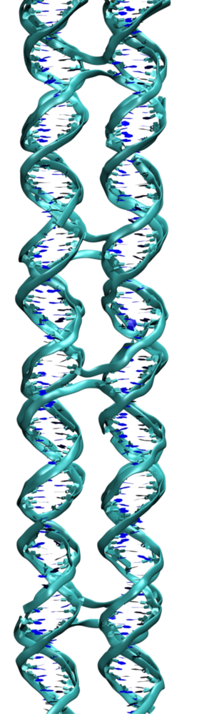
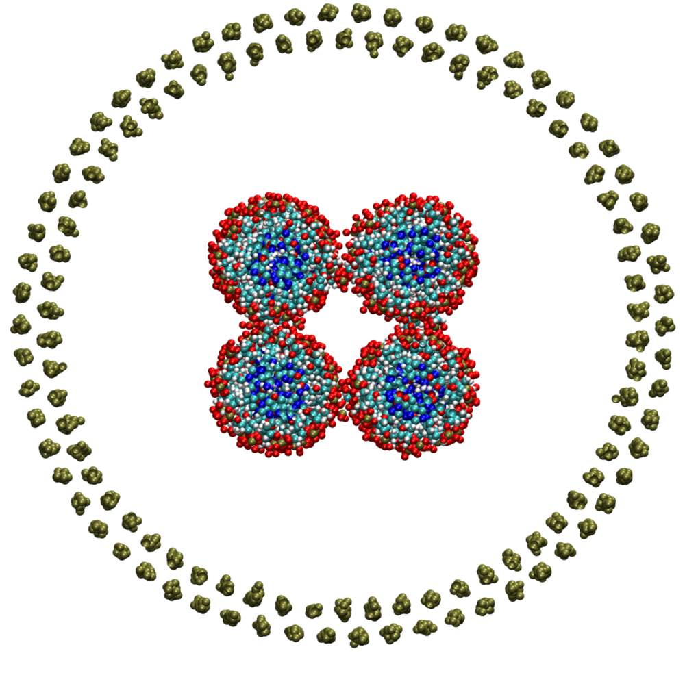
Figure 1: The side view (left) and cross-section (right) of the all-atom origami molecule section in a pore. For clarity the water molecules have been excluded.

II.2 All-atom quad

This model is constructed by placing four parallel strands of the dsDNA described in Ref. Kesselheim, Müller, and Holm, 2014 parallel to each other. The main difference to the model in the previous section is the missing interconnecting staple strands (Fig. 2). Each of the four helices consists of 20 CG base pairs which corresponds to two full turns of the helix. All other simulation parameters have been adopted from the model above.

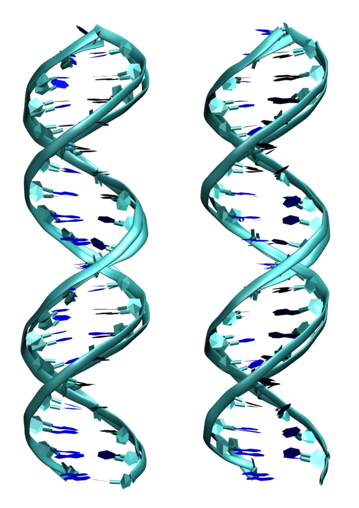
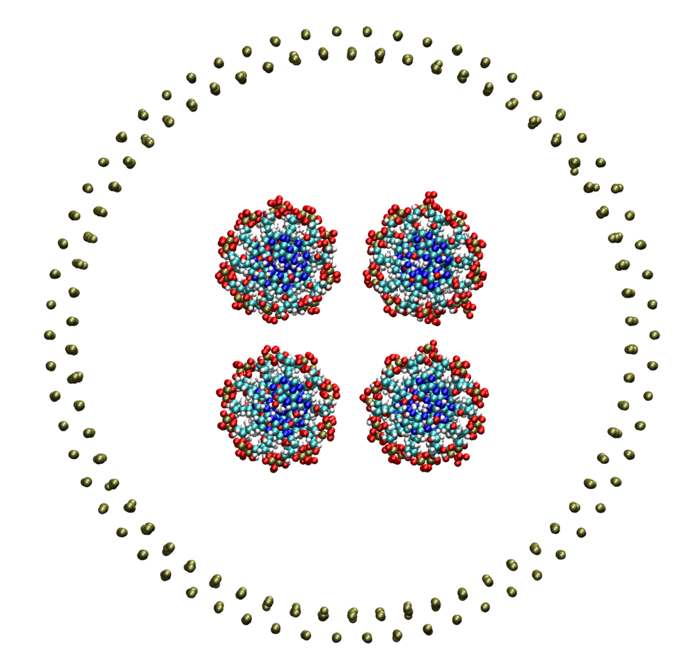
Figure 2: Side view (left) and cross-section (right) of the simulated all-atom quad molecule in a pore.

II.3 Coarse-grained DNA origami

We followed the modelling strategy for a coarse-grained model of a dsDNA molecule as published in Ref. Rau, Weik, and Holm, 2017. In order to extend the model to reproduce the geometry of the origami molecule we created a fixed arrangement of four parallel dsDNA strands (cf. Fig. 4). Simulations have been performed with the release 4.0 of the MD software ESPResSo Weik et al. (2019b).

The segments of the coarse-grained dsDNA consist of a rigid arrangement of three beads (two for the backbone and one for the base pair). A scheme for a single base pair is shown in Fig. 3. Hydrodynamic interactions are included by coupling molecular dynamics with a lattice Boltzmann hydrodynamics solver. Using the point coupling scheme Ahlrichs and Dünweg (1999); Dünweg and Ladd (2009) to exchange momentum between particles and the lattice Boltzmann fluid, a nonphysical fluid flow has been observed along the grooves of the helix Weik, Kesselheim, and Holm (2016) which is suppressed with additional beads that only interact with the fluid and are part of the rigid body of each segment. To match the distance dependent ion mobility in the vicinity of the DNA observed in all-atom simulations Kesselheim, Müller, and Holm (2014), a frictional coupling force $\mathbf{F}_{ij}$ between the backbone particles and the ions is added:

$$\mathbf{F}_{ij}=\begin{cases}-\zeta\left(1-\frac{r_{ij}}{r_{\mathrm{c}}}\right)^{2}\mathbf{v}_{ij},&r_{ij}\leq r_{\mathrm{c}}\\ 0,&\mathrm{else},\end{cases}$$ (1)

where $\zeta$ is a numerical constant, $r_{ij}$ is the inter-particle distance between DNA bead and ion, $r_{\mathrm{c}}$ is the cutoff radius up to which the frictional interaction is enabled, $\mathbf{v}_{ij}$ is the relative velocity. The two free parameters $\zeta$ and $r_{\mathrm{c}}$ are tuned to match the ion velocity profile of the respective all-atom simulation for a single salt concentration. In addition to the frictional force, a random force according to the fluctuation-dissipation theorem is applied. Details of the model can be found in Ref. Rau, Weik, and Holm, 2017, exact values for all parameters are listed in the supporting information.

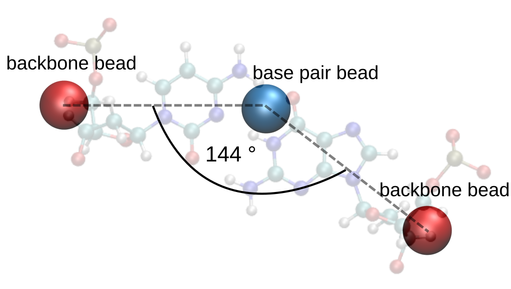
Figure 3: Top view of a single coarse-grained base pair. In the background the respective atomic visualization is shown for comparison. Note, that the beads are not drawn to scale for clarity.

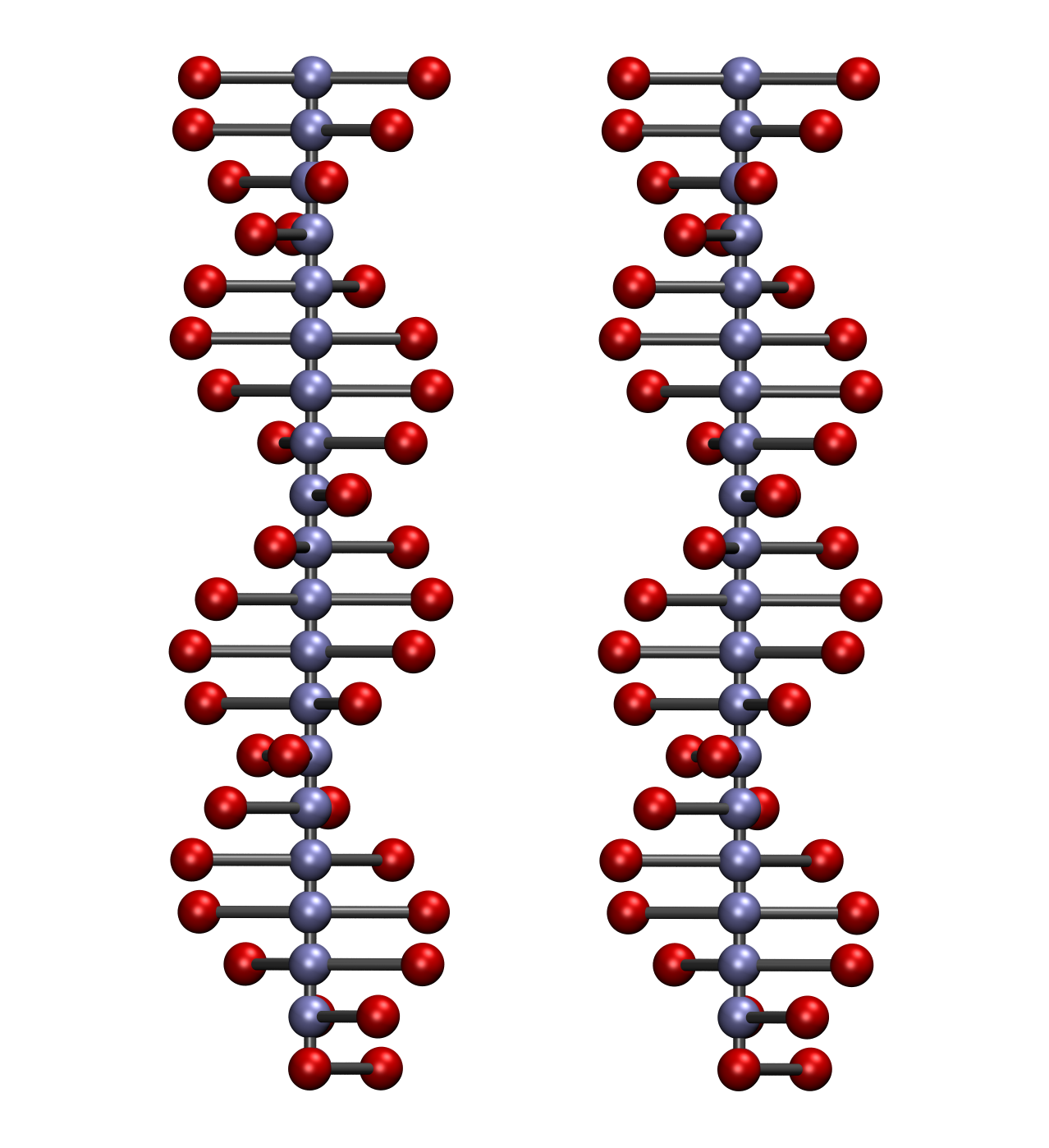
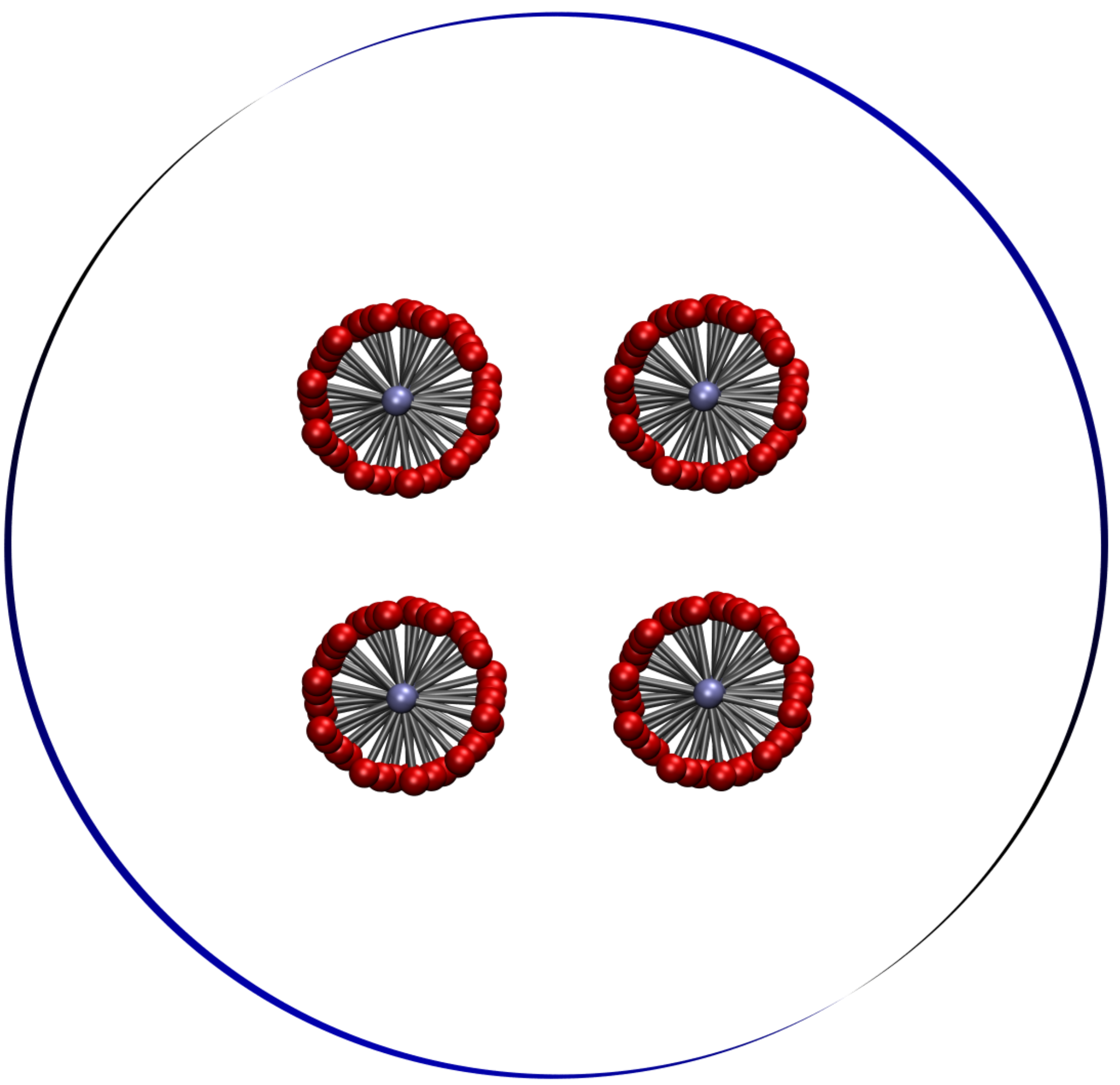
Figure 4: The side view (left) of the coarse-grained quad molecule as developed in Ref. Rau, Weik, and Holm, 2017 and the cross-section (right) of the simulated pore system.

II.4 Mean-field model

Based on the geometric arrangement of the coarse-grained model in the previous section, the DNA strands in the mean-field model are replaced by charged cylinders that carry the respective surface charge density of a dsDNA molecule ($\sigma_{\text{DNA}}\approx$-2\text{\,}\mathrm{\text{ $e$ }}$/$2.35\text{\,}{\mathrm{nm}}^{2}$\approx$-0.136\text{\,}\mathrm{C}\text{\,}{\mathrm{m}}^{-2}$$). It is based on solving the modified electrokinetic equations for the bundle of charged cylinders representing the dsDNA structure within an uncharged cylinder representing the nanopore following the approach in Ref. Weik et al., 2019a. The Nernst-Planck equation is modified to incorporate the friction between ions and dsDNA molecules that has previously been found to be crucial for coarsened dsDNA models in order to reproduce experimental data on current modulation in nanopores Weik, Kesselheim, and Holm (2016). Thus, the algebraic equation for the current density of species $i\in\{\mathrm{K},\mathrm{Cl}\}$ along the symmetry axis reads:

$$j_{i}^{z}=\Biggl{[}\underbrace{\vphantom{\left(\frac{j_{i}^{z}}{c_{i}}\right)}u^{z}}_{\text{advection}}+\mu_{i}\Biggl{(}\underbrace{\vphantom{\left(\frac{j_{i}^{z}}{c_{i}}\right)}ez_{i}E^{z}}_{\text{external field}}\underbrace{\vphantom{\left(\frac{j_{i}^{z}}{c_{i}}\right)}-\alpha\omega\frac{j_{i}^{z}}{c_{i}}}_{\text{friction}}\Biggr{)}\Biggr{]}c_{i},$$ (2)

where $c_{i}$ is the concentration, $u^{z}$ is the fluid velocity, $\mu_{i}$ the ion mobility, $e$ the elementary charge, $z_{i}$ the valency, $E^{z}$ the electric field strength along the symmetry axis, $\alpha=$15\text{\times}{10}^{-12}\text{\,}\mathrm{kg}\text{\,}{\mathrm{s}}^{-1}$$ a numerical constant (controlling the amount of frictional force) and $\omega$ is a position dependent weight function for the frictional force (cf. Ref. Weik et al., 2019a for details).

The advective motion of ions is taken into account by means of the Stokes’ equation and electrostatic interactions between ions are considered following the Poisson-Boltzmann theory. Due to the friction between ions and dsDNA this results in a coupling between electrostatic and advective forces on the ions. The model’s inherent symmetry reduces the problem domain to two dimensions. We solved the electrokinetic equations with the finite-element method using the commercial software package COMSOL Multiphysics^® version 5.4.

Figure 5: Sketch of the geometry used in the mean-field model. Details can be found in Ref. Weik et al., 2019a.

III Results

III.1 Model agreement across scales

In the following, we will compare the salt-dependent current modulation for the four aforementioned models (all-atom origami, all-atom quad, coarse-grained and mean-field model). To get a dimensionless number that we can directly compare across the models, we looked at the relative change in ionic current $I_{\mathrm{mod}}=\left(I_{\mathrm{DNA}}-I_{\mathrm{empty}}\right)/I_{\mathrm{empty}}$, where $I_{\mathrm{DNA}}$ is the current of the pore with the DNA origami molecule inside and $I_{\mathrm{empty}}$ the current of the empty pore with salt only. As shown in Fig. 6, the agreement for the current modulation is very good among the models, taking into account the statistical errors for each model. Especially with regard to the crossover salt concentration $\tilde{c}$ where the relative change in current vanishes ($I_{\mathrm{mod}}(\tilde{c})=0$), the results of the four models agree within a small interval of the bulk salt concentration. The fact that a quantitative agreement for these models has already been observed for a single dsDNA molecule in Refs. Kesselheim, Müller, and Holm, 2014; Rau, Weik, and Holm, 2017; Weik et al., 2019a and the agreement we found in this work for a larger dsDNA bundle structure, suggests that our models would also show consistent results for larger bundle structures, e.g. for a system of 4x4 helices as investigated by Wang et al. in Ref. Wang, Ermann, and Keyser, 2019 (cf. Fig. 10).

In order to investigate the location dependent contribution to the current modulation, the relative current density modulation across the pore $j_{\mathrm{mod}}=\left(j_{\mathrm{DNA}}-j_{\mathrm{empty}}\right)/j_{\mathrm{empty}}$ (naming convention as for $I_{\mathrm{mod}}$) is shown in Fig. 7. In case of the all-atom and the coarse-grained model, the current density for the empty pore has been radially averaged to reduce the noise. For the all-atom quad model, we additionally averaged the current density data for the filled pore by rotating the data by $N\pi/2$ with $N\in\{1,2,3\}$ around the pore center, leveraging the $D_{4}$ symmetry group of the model’s geometry. As expected, we observe a negative current density modulation in the area where the DNA helices are located due to blockage and friction with the ions. In the case of the all-atom origami model, the footprints of the inter-helix connections are visible and neutralize the modulation within a small area. For this model $j_{\mathrm{mod}}$ is larger in the pore center than between two adjacent helices whereas in the case of the all-atom quad model it is the other way around. The two coarser models (coarse-grained and mean-field) without inter-helix connections both show a very similar current density modulation profile compared to the all-atom quad model.

Since the current modulations for all investigated systems show a very good agreement (cf. Fig. 6), the differences in the current density modulation profiles (cf. Fig. 7) have to have the following characteristics: local differences between the models are canceled out by complementary differences in other regions of the pore and these compensating effects either do not depend on the salt concentration or depend on it in a way that preserves the ionic current’s dependency on the salt concentration.

To investigate the current density in greater detail, we additionally analyzed the components that make up the current density, namely the charge density profile and the ion velocity profiles. The charge density profiles shown in Fig. 8 reveal that the all-atom origami system has a slightly higher concentration of charges between adjacent helices but overall the profiles for all four models look very similar. Thus, the charge density profile does not explain the differences in the relative current density modulation we observed for the all-atom origami model (cf. Fig. 7).

The velocity profiles for the molecular dynamics systems (as described in Sec. II.1, II.2, II.3) can be directly computed from the trajectories of the ions. Ion velocities for the mean-field model have been obtained via the following expression:

$$v_{i}(x,y)^{z}=\frac{j_{i}(x,y)^{z}}{c_{i}(x,y)}=\frac{u(x,y)^{z}+\mu_{i}ez_{i}E^{z}}{\alpha\mu\omega(x,y)+1}.$$ (3)

A detailed explanation of the notation can be found in Sec. II.4.

All velocity profiles shown in Fig. 9 are normalized with the respective average ion velocity in the empty pore, thus enabling the direct comparison of the data for the different models. While the velocity profiles for the anions do not show a significant deviation among the models, more prominent differences are visible between the cation (counter-ion) velocity profiles of the all-atom origami and all-atom quad model. Here, the cation velocity in the origami model is larger at the pore center compared to the region between adjacent helices. On the other hand, the opposite relation is observed for the quad model. These differences in the velocity profiles together with the charge density data shown in Fig. 8 thus explain the relative current modulation differences between those two models.

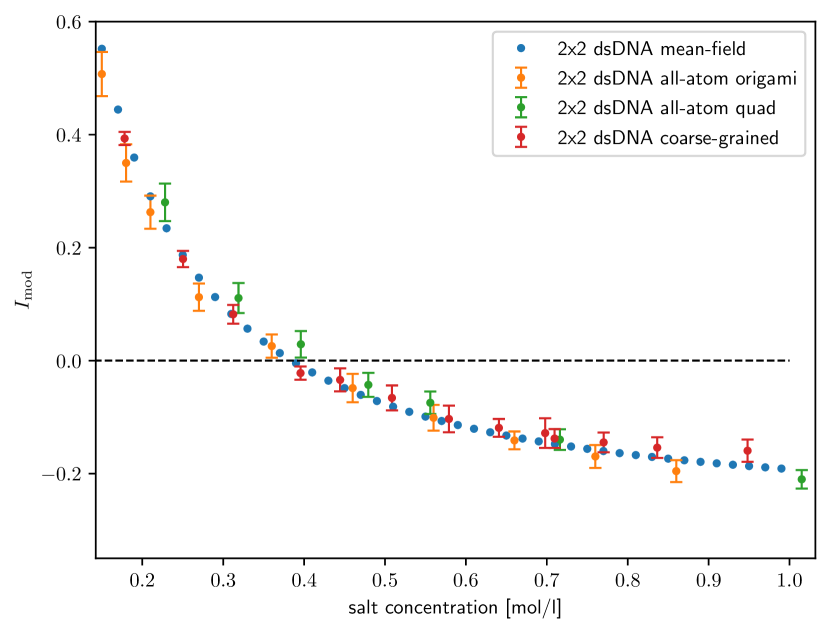
Figure 6: Relative change in ionic current through the nanopore for all four investigated models for a 2x2 dsDNA bundle. The results of all models agree within errors over the whole range of investigated salt concentrations.

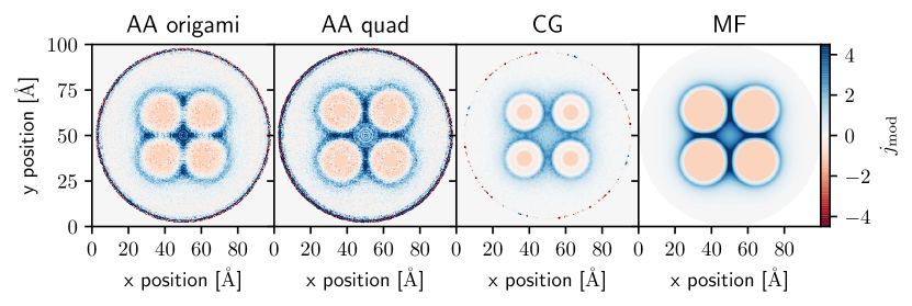
Figure 7: Relative current density modulation for the all-atom (left), the coarse-grained (mid) and the mean-field model (right). The non-vanishing modulation at the pore walls for the all-atom and coarse-grained models can be attributed to large current density fluctuations and poor statistics. The salt concentration for all models was approx. $0.18\text{\,}\mathrm{mol}\text{\,}{\mathrm{l}}^{-1}$.

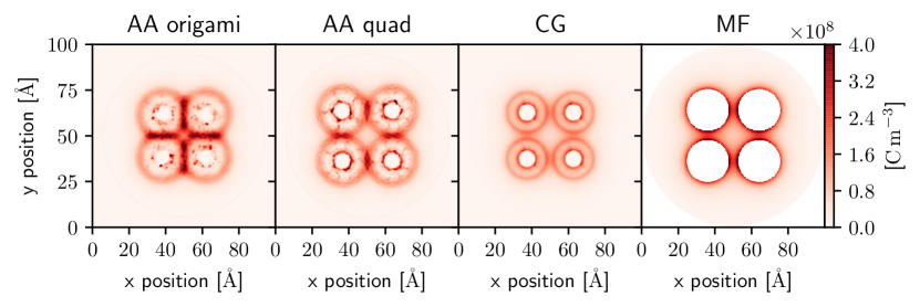
Figure 8: Charge density profiles for the all-atom origami, the all-atom quad, the coarse-grained and the mean-field model at approx. $0.18\text{\,}\mathrm{mol}\text{\,}{\mathrm{l}}^{-1}$.

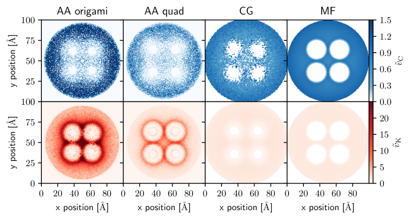
Figure 9: Normalized ion velocity profiles for the anions (top row) and the cations (bottom row) at a salt concentration of approx. $0.18\text{\,}\mathrm{mol}\text{\,}{\mathrm{l}}^{-1}$. The velocities are normalized with the respective empty pore ion velocities in order to get directly comparable dimensionless values.

III.2 Comparison to experimental data

The group of Ulrich Keyser in Cambridge performed experiments in a similar setting Wang, Ermann, and Keyser (2019). They conducted translocation experiments using conical glass nanocapillary pores immersed in solutions of KCl. These nanopores had a mean pore diameter of $14.2\text{\,}\mathrm{nm}$. For comparison, we used $10\text{\,}\mathrm{nm}$ diameter pores in the simulations. However, as shown in a previous publication Weik et al. (2019a) the pore size does not significantly influence the current modulation. The DNA origami molecules of Ref. Wang, Ermann, and Keyser, 2019 have been designed and assembled of 4 or 16 parallel dsDNA double-helices connected by periodically repeating crossover staple strands. Any possible occurrence of electroosmotic flow due to the charged glass walls has been suppressed by adding a tuned amount of polyethylene glycol. Wang et al. reported a much smaller crossover salt concentration $\tilde{c}$($128\text{\,}\mathrm{mmol}\text{\,}{\mathrm{l}}^{-1}$ for the 2x2 origami and $310\text{\,}\mathrm{mmol}\text{\,}{\mathrm{l}}^{-1}$ for dsDNA) compared to similar experimental setups where dsDNA translocation has been investigated Steinbock et al. (2012). Furthermore, they found a non-monotonic behavior of $\tilde{c}$ with respect to the size of the analyte: $\tilde{c}_{\text{dsDNA}}>\tilde{c}_{\text{2x2}}<\tilde{c}_{\text{4x4}}$, i.e. the crossover salt concentration for 4x4 origami molecules is reportedly higher ($183\text{\,}\mathrm{mmol}\text{\,}{\mathrm{l}}^{-1}$) than for the smaller 2x2 origami. From all-atom simulations of an infinite pore system Kesselheim, Müller, and Holm (2014) with a dsDNA molecule it is known that the ionic current is determined by two competing effects: (i) reduction in current due to friction between ions and DNA helices, and (ii) enhanced current due to additional mobile (counter-) ions. The relative importance of these effects for the overall current modulation depends on the bulk salt concentration of the electrolyte and is non-trivial.

Since we now can safely assume that the frictional effects add up linearly, we also investigated a 4x4 origami with our mean-field model. An overview of the salt dependent current modulation for different experimental systems and simulation models is shown in Fig. 10. The data labeled as “mean-field” in the plot legend refers to the respective model as described in Sec. II.4 with varying numbers of charged cylinders representing the different numbers of DNA helices in the model. The current modulation of the three mean-field systems shows a slight monotonic trend towards higher crossover salt concentrations for larger DNA structures (cf. inset of Fig. 10) whereas the experimental results show a large drop of $\tilde{c}$ to smaller salt concentrations from a dsDNA molecule to the 2x2 origami. Furthermore, the 4x4 origami shows an increased value for $\tilde{c}$ compared to the 2x2 in the experiments of Wang et al. Wang, Ermann, and Keyser (2019). Thus, all of our simulation results show a significant deviation for all origami systems despite being accurate for the case of a single DNA molecule as has been shown in Refs. Kesselheim, Müller, and Holm, 2014; Weik, Kesselheim, and Holm, 2016; Rau, Weik, and Holm, 2017; Weik et al., 2019b.

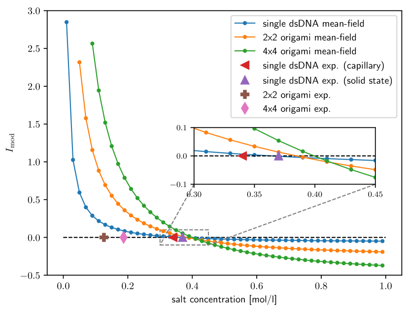
Figure 10: Comparison of the current modulation for different setups. Experimental data taken from Refs. Smeets et al., 2006; Wang, Ermann, and Keyser, 2019.

Comparing the experimental setup to our simulation models, we presume deviations to result from one or combinations of the following simplifications in our models: the pore entrance and the finite molecule lengths are neglected, an alignment of the molecule’s symmetry axis with the pore axis is assumed, and the lateral position of the DNA structure’s symmetry axis is fixed to the pore center.

Regarding the finite pore and analyte effects, a possible deviation might be expected since the 2x2 origami molecule and the 4x4 origami molecule are folded from the same scaffold strand and therefore have a different aspect ratios which may be related to the non-monotonic effect of the molecule’s apparent blocking area on the crossover salt concentration. Moreover, Ref. Wang, Ermann, and Keyser, 2019 speculates about the possibility of a diffusion limited current through the origami structure.

Another possibility is that tilted conformations of the origami molecules might occur that may lead to a higher effective friction between ions and origami and the pore. As the simulations show (cf. Fig. 7), the highest current density is in the counter ion layer around the helices. If these layers come closer to the pore walls, this might also lead to a reduction in pore conductivity. However, due to the like-charge repulsion of the glass capillary and the DNA molecule, we expect this effect to be minor.

The dependency of the pore conductivity on the position of a single dsDNA molecule has already been investigated for the mean-field model in Ref. Weik et al., 2019a. No significant influence of the molecules position on the pore conductivity had been found unless the gap between the DNA molecule and the pore wall is smaller than the Debye length. Since the Debye length is $\approx\frac{1}{10}$ pore diameter at the experimentally reported crossover salt concentration, we do not expect this effect to be significant. Also, as our current density profiles show that a non-negligible portion of the current stems from ions inside the DNA structure which is not directly influenced by the pore walls.

IV Conclusion

We presented a thorough investigation of four simulation models for the current modulation of bundled DNA nanostructures. The coarse-grained and mean-field models were parameterized only for a single dsDNA molecule. Although the level of detail is ranging from the all-atom scale to the mean field scale, we observe a very good agreement among the models with respect to the salt dependent current modulation in a nanopore. This means that the frictional effects are additive for the nanostructures which opens up the door to build arbitrarily large DNA bundles from dsDNA. Spatially resolving the current density across the pore revealed slight different ion mobilities at the center of the pore. While the ion mobilities for the coarse-grained model and the mean-field model are very similar, the all-atom origami model shows a higher ion mobility at the center of the DNA nanostructure. The difference in the current density in the pore center, however, is compensated by slight differences between adjoint helices in the structure. In summary, our study shows that the current modulation for an infinite pore system is robust against changes to molecular details.

Furthermore, we compared our results to recent experiments by Wang et al. Wang, Ermann, and Keyser (2019) This comparison revealed a significant mismatch of the crossover salt concentrations between our models and experimental results (cf. Fig. 10). Compared to a single dsDNA molecule, the experimental results show a much lower ionic current if the bundled DNA structure is in the pore Wang, Ermann, and Keyser (2019). Wang et al. suggested this to be a non-linear effect of the overlapping ion-DNA frictional interaction near the bundled DNA structures. However, we do not observe such a drop in the current density within the structures but a significant increase (compared to the bulk) either between adjoint helices (all-atom quad, coarse-grained and mean-field model) or at the pore center (all-atom DNA origami). The two other possible suggestions for the current reduction in Ref. Wang, Ermann, and Keyser, 2019, namely the idea of a diffusion limitation and end-effects in the pore, cannot be investigated with the models presented here.

A possible way of further investigations could be a model with finite pore and analyte. Such a model may be based on the coarse-grained or the mean-field model we presented here and be extended by additional electrolyte cis- and trans-reservoirs. Investigations along these lines are in progress.

V Acknowledgments

We thank Jonas Landsgesell, Georg Rempfer, Alexander Schlaich and Ulrich Keyser with co-workers for fruitful discussions. The work is funded by the Deutsche Forschungsgemeinschaft (DFG, German Science Foundation) - Project Number 390740016 - EXC 2075. CH, KS, and FW also gratefully acknowledge funding by the collaborative research center SFB 716.

VI Data Availability

The data that support the findings of this study are available from the corresponding author upon reasonable request.

VII Supporting Information

VII.1 DNA origami structure

The DNA origami is a 4-helix bundle composed of a scaffold strand with 7250 nucleobases stabilized by 174 short staple strands. The DNA sequence of these staple strands can be found in Ref. Wang, Ermann, and Keyser, 2019 Table S9. The quaternary structure of the 4-helix bundle has translational symmetry along its main axis with a length of $217.6\text{\,}\mathrm{\SIUnitSymbolAngstrom}$. An image of the unit cell can be found in Fig. 11.

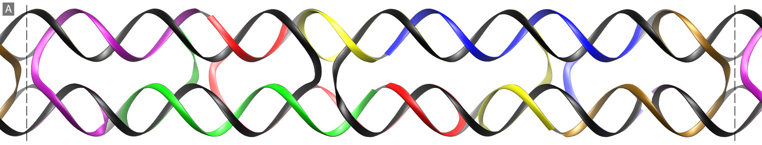
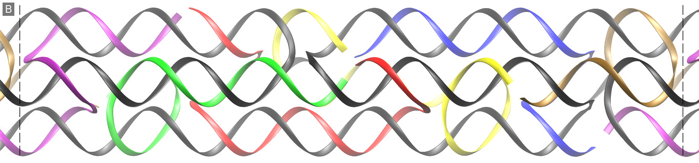
Figure 11: Close-up view of the unit cell from two different perspectives A and B related by a rotation of $45\text{\,}\mathrm{\SIUnitSymbolDegree}$ around the main axis. The dashed lines represent the periodic boundaries. The scaffold strand is colored in black while the 6 linker strands are colored in blue, red, green, yellow, ocher and purple, respectively.

The structure used in this paper contains a segment of the scaffold strand and 7 staple strands: full-length oligomers 9, 10, 67, 119, 150, and fragments of oligomers 66 and 68.

VII.2 Interaction parameters of the coarse-grained model

The mobility reduction observed in all-atom simulations Kesselheim, Müller, and Holm (2014) is modelled via a velocity dependent pair force between the backbone particles of the coarse-grained model and the ions:

$$\mathbf{F}_{ij}=\begin{cases}-\zeta\left(1-\frac{r_{ij}}{r_{\mathrm{c}}}\right)^{2}\mathbf{v}_{ij},&r_{ij}\leq r_{\mathrm{c}}\\ 0,&\mathrm{else},\end{cases}$$ (4)

where $\zeta$ is the friction parameter, $r_{c}$ the cutoff distance, $r_{ij}$ the distance between the particles $i$ and $j$, $\mathbf{v}_{ij}$ is the relative velocity. We chose the two free parameters $r_{c}=$11\text{\,}\mathrm{\SIUnitSymbolAngstrom}$$ and $\zeta=6.25$ such that the velocity profiles between the coarse-grained model and the results from all-atom simulations matched reasonably well.

Furthermore, the non-bonded Lennard-Jones interaction potential has been used to model the excluded volume between particles:

$$\begin{split}U(r_{ij})=\begin{cases}4\epsilon\left[\left(\frac{\sigma}{r_{ij}-r_{\mathrm{off}}}\right)^{12}-\left(\frac{\sigma}{r_{ij}-r_{\mathrm{off}}}\right)^{6}+c\right]&\\ \text{ for }r_{\mathrm{off}}<r_{ij}<r_{\mathrm{c}}+r_{\mathrm{off}}\\ 0,&\mathrm{else},\end{cases}\end{split}$$ (5)

where $\sigma$ is the particle diameter, $r_{ij}$ the distance between the particles, $r_{\mathrm{off}}$ a distance offset, $r_{\mathrm{c}}$ the cutoff distance and $c$ an energy shift. In the following we list the interaction parameters for the different particle pairs of the coarse-grained model.

Table 1: Summary of pair interaction parameters.

interaction pair	$\sigma[$\mathrm{\SIUnitSymbolAngstrom}$]$	$\epsilon[k_{\textnormal{B}}T]$	$r_{\mathrm{cut}}[\sigma]$	$r_{\mathrm{off}}[\sigma]$
ion-ion	4.25	1	$2^{\frac{1}{6}}$	0.0
ion-pore	4.25	1	$2^{\frac{1}{6}}$	0.0
ion-backbone	4.25	1	$2^{\frac{1}{6}}$	0.0
ion-basepair	4.25	1	$2^{\frac{1}{6}}$	0.18

The parameter $c$ in Eq. (5) is chosen such that the interaction potential is zero at the chosen cutoff distance. Since the DNA is fixed in the pore center there is no interaction defined between DNA beads and the pore.

References

- Coulter (1953) W. H. Coulter, “Means for counting particles suspended in a fluid,” (1953), US Patent 2,656,508.
- DeBlois and Bean (1970) R. DeBlois and C. Bean, Review of Scientific Instruments 41, 909 (1970).
- Kasianowicz et al. (1996) J. J. Kasianowicz, E. Brandin, D. Branton, and D. W. Deamer, Proceedings of the National Academy of Sciences 93, 13770 (1996).
- Cherf et al. (2012) G. M. Cherf, K. R. Lieberman, H. Rashid, C. E. Lam, K. Karplus, and M. Akeson, Nature biotechnology 30, 344 (2012).
- Manrao et al. (2012) E. A. Manrao, I. M. Derrington, A. H. Laszlo, K. W. Langford, M. K. Hopper, N. Gillgren, M. Pavlenok, M. Niederweis, and J. H. Gundlach, Nature biotechnology 30, 349 (2012).
- Smeets et al. (2006) R. M. M. Smeets, U. F. Keyser, D. Krapf, M.-Y. Wu, N. H. Dekker, and C. Dekker, Nano Letters 6, 89 (2006).
- Kesselheim, Müller, and Holm (2014) S. Kesselheim, W. Müller, and C. Holm, Physical Review Letters 112, 018101 (2014).
- Weik, Kesselheim, and Holm (2016) F. Weik, S. Kesselheim, and C. Holm, The Journal of Chemical Physics 145, 194106 (2016).
- Weik et al. (2019a) F. Weik, K. Szuttor, J. Landsgesell, and C. Holm, The European Physical Journal Special Topics 227, 1639 (2019a).
- van Dorp et al. (2009) S. van Dorp, U. F. Keyser, N. H. Dekker, C. Dekker, and S. G. Lemay, Nat Phys 5, 347 (2009).
- Luan and Aksimentiev (2008) B. Luan and A. Aksimentiev, Physical Review E 78, 021912 (2008).
- Castro et al. (2011) C. E. Castro, F. Kilchherr, D.-N. Kim, E. L. Shiao, T. Wauer, P. Wortmann, M. Bathe, and H. Dietz, Nature methods 8, 221 (2011).
- Han et al. (2011) J. Han, E. Haihong, G. Le, and J. Du, in Pervasive computing and applications (ICPCA), 2011 6th international conference on (IEEE, 2011) pp. 363–366.
- Yoo and Aksimentiev (2013) J. Yoo and A. Aksimentiev, Proceedings of the National Academy of Sciences 110, 20099 (2013).
- Bell et al. (2012) N. A. W. Bell, C. R. Engst, M. Ablay, G. Divitini, C. Ducati, T. Liedl, and U. F. Keyser, Nano Letters 12, 512 (2012), http://pubs.acs.org/doi/pdf/10.1021/nl204098n .
- Langecker et al. (2012) M. Langecker, V. Arnaut, T. G. Martin, J. List, S. Renner, M. Mayer, H. Dietz, and F. C. Simmel, Science 338, 932 (2012).
- Wei et al. (2012) R. Wei, T. G. Martin, U. Rant, and H. Dietz, Angewandte Chemie International Edition 51, 4864 (2012), https://onlinelibrary.wiley.com/doi/pdf/10.1002/anie.201200688 .
- Hernández-Ainsa et al. (2013) S. Hernández-Ainsa, N. A. Bell, V. V. Thacker, K. Gooepfrich, K. Misiunas, M. E. Fuentes-Perez, F. Moreno-Herrero, and U. F. Keyser, ACS Nano 7, 6024 (2013).
- Hernández-Ainsa et al. (2014) S. Hernández-Ainsa, K. Misiunas, V. V. Thacker, E. A. Hemmig, and U. F. Keyser, Nano letters 14, 1270 (2014).
- Göpfrich et al. (2016) K. Göpfrich, C.-Y. Li, M. Ricci, S. P. Bhamidimarri, J. Yoo, B. Gyenes, A. Ohmann, M. Winterhalter, A. Aksimentiev, and U. F. Keyser, ACS nano 10, 8207 (2016).
- Li et al. (2015) C.-Y. Li, E. A. Hemmig, J. Kong, J. Yoo, S. Hernández-Ainsa, U. F. Keyser, and A. Aksimentiev, ACS nano 9, 1420 (2015).
- Barati Farimani, Dibaeinia, and Aluru (2017) A. Barati Farimani, P. Dibaeinia, and N. R. Aluru, ACS Applied Materials & Interfaces 9, 92 (2017).
- Wang, Ermann, and Keyser (2019) V. Wang, N. Ermann, and U. F. Keyser, Nano Letters 19, 5661 (2019), https://doi.org/10.1021/acs.nanolett.9b02219 .
- Steinbock et al. (2012) L. J. Steinbock, A. Lucas, O. Otto, and U. F. Keyser, Electrophoresis 33, 3480 (2012).
- Duan et al. (2003) Y. Duan, C. Wu, S. Chowdhury, M. C. Lee, G. Xiong, W. Zhang, R. Yang, P. Cieplak, R. Luo, T. Lee, J. Caldwell, J. Wang, and P. Kollman, Journal of Computational Chemistry 24, 1999 (2003).
- Smith and Dang (1994) D. E. Smith and L. X. Dang, Journal of Chemical Physics 100, 3757 (1994).
- Berendsen, Grigera, and Straatsma (1987) H. J. C. Berendsen, J. R. Grigera, and T. P. Straatsma, The Journal of Physical Chemistry 91, 6269 (1987).
- Abraham et al. (2015) M. J. Abraham, T. Murtola, R. Schulz, S. Páll, J. C. Smith, B. Hess, and E. Lindahl, SoftwareX 1, 19 (2015).
- Rau, Weik, and Holm (2017) T. Rau, F. Weik, and C. Holm, Soft Matter 13, 3918 (2017).
- Weik et al. (2019b) F. Weik, R. Weeber, K. Szuttor, K. Breitsprecher, J. de Graaf, M. Kuron, J. Landsgesell, H. Menke, D. Sean, and C. Holm, The European Physical Journal Special Topics 227, 1789 (2019b).
- Ahlrichs and Dünweg (1999) P. Ahlrichs and B. Dünweg, Journal of Chemical Physics 111, 8225 (1999).
- Dünweg and Ladd (2009) B. Dünweg and A. J. C. Ladd, in Advanced Computer Simulation Approaches for Soft Matter Sciences III, Advances in Polymer Science, Vol. 221 (Springer-Verlag Berlin, Berlin, Germany, 2009) pp. 89–166.
- Note (1) The impression of different pore diameters is an interpolation artifact due to different bin sizes.