Testing Quantum Coherence in Stochastic Electrodynamics with Squeezed Schrödinger Cat States

Abstract

The interference pattern in electron double-slit diffraction is a hallmark of quantum mechanics. A long standing question for stochastic electrodynamics (SED) is whether or not it is capable of reproducing such effects, as interference is a manifestation of quantum coherence. In this study, we use excited harmonic oscillators to directly test this quantum feature in SED. We use two counter-propagating dichromatic laser pulses to promote a ground-state harmonic oscillator to a squeezed Schrödinger cat state. Upon recombination of the two well-separated wavepackets, an interference pattern emerges in the quantum probability distribution but is absent in the SED probability distribution. We thus give a counterexample that rejects SED as a valid alternative to quantum mechanics.

I Introduction

Over the past decades, there has been sustained interest in developing classical alternatives to quantum mechanics (QM) with the goal of solving the quantum-classical boundary problem. Despite the proposed classical alternatives Pena1996 ; Pena2015 ; Cavalleri , there is a lack of quantitative tests of such theories against QM, mostly because analytic solutions to concrete physical systems such as two-level atoms have not be found. Arguably one of the most developed classical alternatives is stochastic electrodynamics (SED) Milonni ; Boyer1975-1 . Studies of SED harmonic systems have found many examples that are in exact agreement with QM. These include the retarded van der Waals force Boyer1973 , ground state distribution of harmonic oscillators Boyer1975-2 ; Huang2013 , Landau diamagnetism Boyer1980 ; Boyer2016 , Planck spectrum of blackbody radiation Boyer1984 ; Boyer2017 , and Debye specific-heat law for solids Santos . Numerical studies of hydrogen have given some qualitative features Puthoff ; Cole , but have not led to a clear success Nieuwenhuizen2015 ; Nieuwenhuizen2016 . Recently, it was further shown that parametric interaction can give rise to discrete SED excitation spectra that is in excellent agreement with QM predictions Huang2015 .

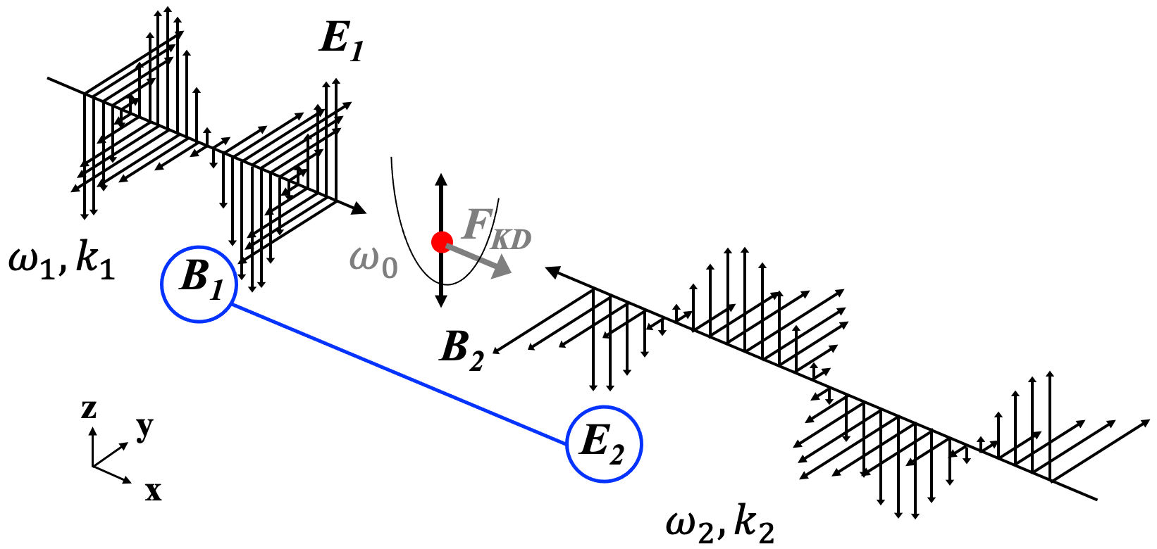
Figure 1: Two counter-propagating laser fields with frequencies $\omega_{1}$ and $\omega_{2}$, collaboratively drive the harmonic oscillator with a spatially modulated Kapitza-Dirac force in the direction of wave propagation. The force has a modulation periodicity of $2\pi c/(\omega_{1}+\omega_{2})$ and it oscillates at the difference frequency $\omega_{1}-\omega_{2}$. A particle subject to the perturbation of the classical zero-point electromagnetic field can get pushed to either directions.

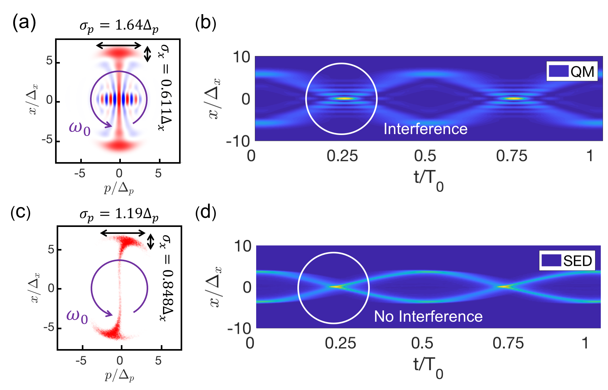
Figure 2: Time evolution of QM and SED probability distributions after laser excitation. (a) The Wigner function of the QM oscillator is plotted after the laser excitation. Positive values are color coded in red and negative values are in blue. Quantum coherence between the two well-separated squeezed states is manifested by the fringe structure in the center. The Wigner function rotates counter-clockwise at the oscillator’s resonant frequency $\omega_{0}=10^{16}$ (rad/s). At the moment when the distribution is depicted, the position quadrature uncertainty $\sigma_{x}$ of the squeezed state is smaller than that of the ground state $\Delta_{x}=\sqrt{\hbar/2m\omega_{0}}$. Meanwhile, the quadrature uncertainty product satisfies the Heisenberg relation $\sigma_{x}\sigma_{p}=\hbar/2$ at all times. (b) The two wavepackets oscillate back and forth in the harmonic potential giving rise to a double sinusoidal trajectory of the QM probability distribution. An interference pattern appears when the two wavepackets merge. (c) The phase space distribution of the SED oscillator shows two well-separated sub-ensembles. Each sub-ensemble has a squeezed structure that mimics the QM squeezed state shown in (a). (d) As the SED phase space distribution rotates counter-clockwise, the probability distribution bundles into two ”macroscopic” trajectories. In each trial of the SED simulation, there is no knowledge which macroscopic trajectory a particle will follow unless the initial phase of the background zero-point field is known. No interference-like patterns are found in the SED probability distribution when the two macroscopic trajectories of distributions cross.

However, a major drawback to the generality of the SED approach is that none of the investigated effects involves quantum coherence. In light of this, some have proposed to study electron double-slit diffraction within the framework of SED as interference is a manifestation of quantum coherence Boyer1975-1 ; Huang2013 ; Bach . Within the SED community the proposed view of electron diffraction is that the double-slit poses boundary conditions that modify the classical zero-point electromagnetic field and in turn it acts as a guiding wave for free electrons Cavalleri ; Boyer1975-1 ; Avendano ; Kracklauer1992 . The appeal of this idea is that the guiding field can be affected by both slits, while the particle passes through only one slit, similar to the idea that has pushed oil droplet analogues Wolchover ; Couder ; Andersen ; Bohr ; Batelaan2016 ; Pucci . As appealing as the idea may sound, so far there has been no concrete calculation or simulation demonstrating such an effect because of two major theoretical obstacles: (1) the effective spectrum of the zero-point field is unbounded for free electrons, (2) The radiation damping of free electrons gives rise to runaway solutions.

Rather than focusing on the specific theoretical difficulties that are relevant to free electrons, we develop a paradigm that can be used as a direct test for quantum coherence in stochastic electrodynamics. Building on our previous results Huang2013 ; Huang2015 , we devise a laser excitation scheme to promote a ground-state quantum harmonic oscillator to a squeezed Schrödinger cat state Kienzler ; Etesse ; Huang . The Schrödinger cat state of a harmonic oscillator is an analogy to the electron double-slit state, $|L\rangle+|R\rangle$, where $|L\rangle$ and $|R\rangle$ indicate the left and right electron slit states in the position space Bach ; Tonomura . Comparing the QM probability distribution with that of SED harmonic oscillators, we observe some interesting similarities. Nevertheless, the interference pattern is missing in the SED probability distribution.

II Kapitza-Dirac force on harmonic oscillators

Let us consider the setup in FIG. 1. Two counter-propagating laser fields propagate along the $x$-axis, and the electric fields are linearly polarized along the $z$-axis,

$$\begin{split}\mathbf{E}_{1}=&A_{1}\omega_{1}\cos{(k_{1}x-\omega_{1}t)}\hat{\epsilon}_{z}\\ \mathbf{E}_{2}=&-A_{2}\omega_{2}\cos{(k_{2}x+\omega_{2}t)}\hat{\epsilon}_{z},\end{split}$$ (1)

where $\hat{\epsilon}_{z}$ is the unit vector along the $z$-axis, $k_{1,2}=\omega_{1,2}/c$ are the wave numbers, and $A_{1,2}$ are amplitudes of the corresponding vector potentials $\mathbf{A}_{1}=A_{1}\sin{(k_{1}x-\omega_{1}t)}\hat{\epsilon}_{z}$ and $\mathbf{A}_{2}=A_{2}\sin{(k_{2}x+\omega_{2}t)}\hat{\epsilon}_{z}$. The electric and magnetic components of the combined laser field are

$$\begin{split}E_{z}=A_{1}\omega_{1}\cos{(k_{1}x-\omega_{1}t)}-A_{2}\omega_{2}\cos{(k_{2}x+\omega_{2}t)}\\ B_{y}=-A_{1}k_{1}\cos{(k_{1}x-\omega_{1}t)}-A_{2}k_{2}\cos{(k_{2}x+\omega_{2}t)}.\end{split}$$ (2)

Assuming that the particle is free in the direction of the electric field (i.e. the $z$-axis in FIG. 1), the cross terms between the electric and magnetic components can give rise to a spatially modulated force in the direction of wave propagation (i.e. the $x$-axis in FIG. 1). Herein we term this force the Kapitza-Dirac (KD) force. The KD force can be derived using the following equations of motion,

$$\left\{\begin{array}[]{l}\displaystyle m\frac{dv_{z}}{dt}=qE_{z}\\ \\ \displaystyle F^{(\textrm{KD})}_{x}=qv_{z}B_{y}\end{array}\right.,$$ (3)

where $m$ and $q$ are mass and charge of the particle. Now, there are two scenarios: (1) if frequencies of the two laser fields are identical ($\omega_{1}=\omega_{2}$), the KD force will be constant in time, which is also known as the pondermotive force Batelaan2007 , (2) if the laser frequencies are different ($\omega_{1}\neq\omega_{2}$), the KD force will oscillate in time with the sum and difference frequencies, $\omega_{1}+\omega_{2}$ and $\omega_{1}-\omega_{2}$. If the charge particle is confined by a harmonic potential $U(x)=m\omega_{0}^{2}x^{2}/2$ with a resonant frequency $\omega_{0}=(\omega_{1}-\omega_{2})/2$, the KD force that can resonantly drive the harmonic oscillator will be (see derivation in Appendix)

$$F_{\textrm{KD}}=\frac{q^{2}A_{1}A_{2}}{m}\left(\frac{k_{1}+k_{2}}{2}\right)\sin{\left((k_{1}+k_{2})x\right)}\cos{\left((\omega_{1}-\omega_{2})t\right)}.$$ (4)

Accordingly, the corresponding time-varying KD potential is

$$U_{\textrm{KD}}=\frac{q^{2}A_{1}A_{2}}{2m}\cos{\left((k_{1}+k_{2})x\right)}\cos{\left((\omega_{1}-\omega_{2})t\right)}.$$ (5)

We note that at any given time $t=t_{0}$ a trapping site in the KD potential $U_{\textrm{KD}}(x,t_{0})$ (i.e. a minimum in the potential) will turn into an unstable point after a quarter of the natural period $T_{0}/4=\pi/|\omega_{1}-\omega_{2}|$, where $T_{0}=2\pi/\omega_{0}$, since the potential polarity is reversed,

$$U_{\textrm{KD}}(x,t_{0}+T_{0}/4)=-U_{\textrm{KD}}(x,t_{0}).$$ (6)

This feature will later be used to coherently split the ground-state wavepacket of a quantum oscillator.

III Generation of squeezed Schrödinger cat states

The KD effect for quantum harmonic oscillators can be modeled by adding the KD potential in Eq. (5) to the unperturbed oscillator Hamiltonian. We replace the continuous-wave laser fields in Eq. (1) with pulsed fields,

$$\begin{split}\mathbf{E}_{1}(x,t)&=A_{1}\omega_{1}\cos{(k_{1}x-\omega_{1}t)}e^{-(t/\tau)^{2}}{\hat{\epsilon}_{z}}\\ \mathbf{E}_{2}(x,t)&=-A_{2}\omega_{2}\cos{(k_{2}x+\omega_{2}t)}e^{-(t/\tau)^{2}}{\hat{\epsilon}_{z}},\end{split}$$ (7)

where $\tau$ is the pulse duration, in order to avoid indefinite sequential excitation of the oscillator’s ladder levels. Given the appropriate pulse amplitudes and durations, the final population distribution can have a peaked structure. The quantum Hamiltonian is thus

$$\hat{H}=\frac{m\omega_{0}}{2}\hat{x}^{2}+\frac{\hat{p}^{2}}{2m}+U_{KD}(\hat{x},t)e^{-2(t/\tau)^{2}}.$$ (8)

The difference frequency of the laser fields is twice the oscillator’s resonant frequency $\omega_{1}-\omega_{2}=2\omega_{0}$, so the ground-state oscillator will be parametrically excited to the even-symmetry states $|n=2k\rangle$, which is a prerequisite for cat state generation because a cat state has an even symmetry. We obtained the QM result by numerically solving the Schödinger equation as in Huang2015 . The oscillator’s parameters are $m=9.11\times 10^{-35}$ (kg), $q=1.60\times 10^{-19}$ (C), and $\omega_{0}=10^{16}$ (rad/s). The laser parameters are chosen to be $\omega_{1}=2.3\,\omega_{0}$, $\omega_{2}=0.3\,\omega_{0}$, $\tau=5\times 10^{-15}$ (s), and $A_{1}=A_{2}=4.5\times 10^{-8}$ (V$\cdot$s/m). The mass is chosen at this unusual value in order to make the computational time for SED simulation more manageable Huang2013 . In FIG. 2(b) the probability trajectory of the excited state is shown. Upon excitation the ground-state wavepacket is coherently split into two wavepackets, so the oscillator is in a superposition of two macroscopically distinct states. The two wavepackets oscillate back and forth in the harmonic potential. As they recombine, interference fringes emerge in the probability distribution due to the quantum coherence between the two wavepackets. The quantum coherence is readily illustrated by the fringe structure in the oscillator’s Wigner function as shown in FIG. 2(a). We note that one of the two quadrature uncertainties of each wavepacket, $\sigma_{x}\equiv\sqrt{\langle x^{2}\rangle-\langle x\rangle^{2}}$ (or $\sigma_{p}\equiv\sqrt{\langle p^{2}\rangle-\langle p\rangle^{2}}$), is smaller than the ground state uncertainty $\Delta_{x}=\sqrt{\hbar/2m\omega_{0}}$ (or $\Delta_{p}=\sqrt{\hbar m\omega_{0}/2}$), while their product remains the same, $\sigma_{x}\sigma_{p}=\hbar/2$, at all times (see FIG. 2(a)). This implies that the state generated by the laser excitation is a squeezed Schrödinger cat state (that is, a superposition of two displaced squeezed states with opposite phases) Etesse ; Huang .

For SED oscillators, we first prepare the classical ensemble in a ground state with the $x$ and $p$ probability distributions identical to those of a quantum oscillator (see details in Huang2013 ). Under excitation of the same laser pulses, the equation of motion for the SED harmonic oscillator is

$$m\frac{d^{2}x}{dt^{2}}=-m\omega_{0}^{2}x-m\Gamma\omega_{0}^{2}\frac{dx}{dt}+qE^{(x)}_{vac}(x,t)+F_{\textrm{KD}}(x,t)e^{-2(t/\tau)^{2}},$$ (9)

where $\displaystyle\Gamma\equiv\frac{2q^{2}}{3mc^{3}}\frac{1}{4\pi\epsilon_{0}}$ is the radiation damping coefficient. The zero-point field $E^{(x)}_{vac}(x,t)$ is configured according to Huang2013 . Apart from the damping term $m\Gamma\omega_{0}^{2}dx/dt$ and the coupling to the zero-point field $E^{(x)}_{vac}(x,t)$, Eq. (9) is formally equivalent to a quantum Heisenberg equation derived from the Hamiltonian in Eq. (8). This suggests that the excitation dynamics in SED should be identical to QM assuming (1) the pulse duration $\tau$ is much shorter than the damping time $\tau_{d}=2/\Gamma\omega_{0}^{2}$, and (2) the KD force is much stronger than the fluctuating force from the zero-point field Huang2013 ,

$$\frac{q^{2}A_{1}A_{2}}{m}\left(\frac{k_{1}+k_{2}}{2}\right)\gg\frac{q}{2\pi}\sqrt{\frac{\hbar\Gamma\omega_{0}^{5}}{\epsilon_{0}c^{3}}}.$$ (10)

In our simulation these two conditions are satisfied, and the excitation dynamics in SED and QM are the same as shown in FIG. 3(a), where the time evolutions of the expectation value of the QM energy and the ensemble average of the SED energy are compared. The two energy trajectories stay overlapped through most of the pulse and only deviate at the end of the excitation. Furthermore, the SED and QM energy distributions have similar shapes (see FIG. 3(b)), despite that the QM distribution is discrete and the SED distribution is continuous.

The probability trajectory of the SED oscillator ensemble along with its phase space distribution are shown in FIG. 2(c)(d). The ensemble particle number is $N_{p}=3\times 10^{4}$. The parametric interaction between the SED oscillator and the laser fields were simulated using the same method as in Huang2015 . Like the QM oscillator, upon excitation the ground-state SED probability distribution also splits into two sub-ensembles that follow two distinct sinusoidal trajectories. The initial phase spectrum of the zero-point field, which is random and considered as the“hidden variable”, determines which trajectory a particle will follow in each trial. A detailed comparison between SED and QM probability distributions is given in FIG. 4 for two time points: (1) when the two QM wavepackets are separated, (2) when they recombine. Although there are some overall similarities between the SED and QM distributions, there are no interference fringes in the SED probability distribution.

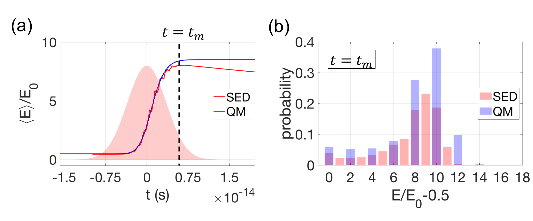
Figure 3: The QM and SED energy distributions after laser excitation. (a) The ensemble average of the SED oscillator energy (red line) is compared with the expectation value of the QM oscillator energy (blue line) during the course of laser excitation. The shaded area (red) represents the excitation laser pulse $e^{-(t/\tau)^{2}}$. The pulse duration is $\tau=5\times 10^{-15}$(s) which is much smaller than the SED oscillator damping time $\tau_{d}\approx 3.2\times 10^{-13}$ (s). Therefore, damping has no significant effect on the oscillator’s dynamics during the excitation process. (a) Energy distributions of QM and SED oscillators are compared at $t=t_{m}$ when the SED energy reaches its maximum and the radiation damping starts to dominate. The QM energy distribution (blue bar) is discrete and occupies only even energy levels $E_{2k}=E_{0}(2k+1/2)$, where $E_{0}=\hbar\omega_{0}$. The SED energy distribution (red bar) is continuous but has a similar width and average value as the QM distribution. This indicates that the excitation process is identical for QM and SED oscillators.

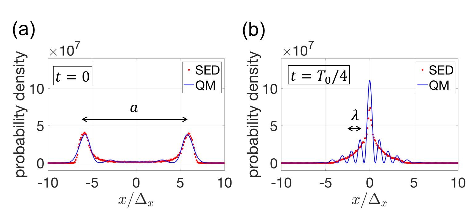
Figure 4: Comparison between the QM and SED probability distributions at $t=0$ and $t=T_{0}/4$ in FIG. 2. (a) The agreement between QM and SED probability distributions is good when the two macroscopically distinct QM wavepackets are well-separated by a peak-to-peak distance $a$ beyond the ground state width $\Delta_{x}$, $a\gg\Delta_{x}$. (b) After a quarter of the natural period $T_{0}/4$, the two QM wavepackets recombine in the harmonic potential. Interference fringes appear in the QM distribution (blue line) but not in the SED distribution (red dots). The fringe periodicity $\lambda$ is determined by the wavepacket separation $a$ in (a) through the relation $\lambda=2\pi\hbar/m\omega_{0}a$, which resembles the well-known double-slit diffraction formula. The SED probability distribution captures the outline of the QM distribution as if the quantum coherence between the two QM wavepackets is lost.

IV Discussion and Conclusion

While the zero-point electromagnetic field only introduces small radiative corrections to nonrelativistic QM, such as Lamb shifts, it drastically changes the particle dynamics in classical mechanics and leads to the reproduction of QM effects in some classical systems Boyer1973 ; Boyer1975-2 ; Huang2013 ; Boyer1980 ; Boyer1984 ; Boyer2017 ; Santos ; Huang2015 . Our work aims to investigate to what extent such a classical theory can reproduce QM features by comparing results obtained from SED, Eq. (9), with those obtained from the QM Hamiltonian, Eq. (8). The qualitative difference between the probability distributions of QM and SED in FIG. 2 and FIG. 4(b) establishes that SED in its traditional form does not support physical effects that involve quantum coherence Milonni ; Boyer1975-1 . The squeezed Schrödinger cat state used in this work is an analogy to the electron double-slit experiment Bach . The peak-to-peak separation $a$ between the two wavepackets in FIG. 4(a) determines the fringe periodicity $\lambda$ in FIG. 4(b) through the relation $\lambda=2\pi\hbar/m\omega_{0}a$, which mimics the double-slit diffraction formula. Our analysis provides evidence that coherence-like behavior is absent in SED, and thus we predict that SED electron double-slit diffraction, if ever calculated, will not show fringes.

On the other hand, our result helps to establish the validity range of SED. We note that the partial agreement between the SED and QM results stems from the formal resemblance between the SED equation of motion and the QM Heisenberg equation assuming that the laser excitation pulses satisfy certain criteria. While $x$ and $p$ are independent dynamic variables in SED, the canonical commutation relation $[\hat{x},\hat{p}]=i\hbar$ makes them a Fourier pair in QM. This difference makes the distinction between QM and SED in terms of quantum coherence. Therefore, SED may be seen as the decoherence limit of QM Sonnentag . Although the zero-point field bestows a special phase relation between $x$ and $p$ of a SED harmonic oscillator, which leads to the quantum ground-state distributions Boyer1975-2 ; Huang2013 , the phase relation serves only as initial conditions and does not affect the dynamical evolution of $x$ and $p$ during laser excitation. Therefore, we speculate that any mechanism or theoretical operation that restores (or deteriorates) the Fourier relation between $x$ and $p$ for SED (or QM), will make the proper decoherence theory that bridges the gap between SED and QM.

V Acknowledgement

The authors thank A. M. Steinberg, C. Monroe, and P. W. Milonni, for advice. W. C. Huang wishes to give special thanks to Yanshuo Li for helpful discussions. This work utilized high-performance computing resources from the Holland Computing Center of the University of Nebraska. We gratefully acknowledge funding support from NSF PHY-1602755.

*

Appendix A Derivation of the resonant Kapitza-Dirac force

In this appendix we derive the KD force in Eq. (4) from Eq. (3) using the electric and magnetic components of the combined laser field given in Eq. (2). First, we solve the velocity $v_{z}$ by integrating the equation of motion $mdv_{z}/dt=qE_{z}$,

$$v_{z}(t)=-\frac{q}{m}\left(A_{1}\sin{(k_{1}x-\omega_{1}t)}+A_{2}\sin{(k_{2}x+\omega_{2}t)}\right).$$ (11)

Substituting $v_{z}(t)$ to $F_{x}=qv_{z}B_{y}$, we obtain the Lorentz force

$$\begin{split}F_{x}=&\frac{q^{2}}{m}\left(A_{1}\sin{(k_{1}x-\omega_{1}t)}+A_{2}\sin{(k_{2}x+\omega_{2}t)}\right)\\ &\times\left(A_{1}k_{1}\cos{(k_{1}x-\omega_{1}t)}+A_{2}k_{2}\cos{(k_{2}x+\omega_{2}t)}\right).\end{split}$$ (12)

We can see four frequency components in the Lorentz force by expanding Eq. (12),

$$\begin{split}F_{x}=&\frac{q^{2}}{2m}\left[A_{1}^{2}k_{1}\sin{(2k_{1}x-2\omega_{1}t)}\right.\\ &+A_{1}A_{2}k_{1}\left(\sin{((k_{1}+k_{2})x-(\omega_{1}-\omega_{2})t)}-\sin{((k_{1}-k_{2})x-(\omega_{1}+\omega_{2})t)}\right)\\ &+A_{1}A_{2}k_{2}\left(\sin{((k_{1}+k_{2})x-(\omega_{1}-\omega_{2})t)}+\sin{((k_{1}-k_{2})x-(\omega_{1}+\omega_{2})t)}\right)\\ &+\left.A_{1}^{2}k_{2}\sin{(2k_{2}x+2\omega_{2}t)}\right].\end{split}$$ (13)

Because the frequency components $2\omega_{1}$, $2\omega_{2}$, and $\omega_{1}+\omega_{2}$ are not integer multipliers of $\omega_{0}$, we can drop these terms and keep only the parametrically resonant term $\omega_{1}-\omega_{2}=2\omega_{0}$,

$$F_{x}\approx\frac{q^{2}}{2m}A_{1}A_{2}(k_{1}+k_{2})\sin{((k_{1}+k_{2})x-(\omega_{1}-\omega_{2})t)}.$$ (14)

The force has a traveling wave profile which can be decomposed into two standing-wave components with even and odd symmetries,

$$\sin{((k_{1}+k_{2})x-(\omega_{1}-\omega_{2})t)}=\sin{((k_{1}+k_{2})x)}\cos{((\omega_{1}-\omega_{2})t)}-\cos{((k_{1}+k_{2})x)}\sin{((\omega_{1}-\omega_{2})t)}.$$ (15)

The force needs to have a potential profile with even symmetry in order to resonantly drive the oscillator from the ground state with an even frequency ($\omega_{1}-\omega_{2}=2\omega_{0}$). This implies that the resonant KD force should an odd symmetry, thus it takes the form

$$F_{KD}=\frac{q^{2}}{2m}A_{1}A_{2}(k_{1}+k_{2})\sin{((k_{1}+k_{2})x)}\cos{((\omega_{1}-\omega_{2})t)}.$$ (16)

References

- (1) L. de la Peña and A. M. Cetto, The Quantum Dice: an Introduction to Stochastic Electrodynamics, Springer (1996).
- (2) L. de la Peña, A. M. Cetto, A. Valdes-Hernandez, Emerging Quantum: the physics behind quantum mechanics, Springer (2015).
- (3) G. Cavalleri et al., Front. Phys. China 5, 107 (2010).
- (4) P. W. Milonni, The Quantum Vacuum: An Introduction to Quantum Electrodynamics, Academic Press (1994).
- (5) T. H. Boyer, Phys. Rev. D 11, 790 (1975).
- (6) T. H. Boyer, Phys. Rev. A 7, 1832 (1973).
- (7) T. H. Boyer, Phys. Rev. D 11, 809 (1975).
- (8) W. C. Huang and H. Batelaan, J. Comput. Methods Phys. 2013, 308538 (2013).
- (9) T. H. Boyer, Phys. Rev. A 21, 66 (1980).
- (10) T. H. Boyer, Eur. J. Phys. 37, 065102 (2016).
- (11) T. H. Boyer, Phys. Rev. D 29, 1096 (1984).
- (12) T. H. Boyer, Eur. J. Phys. 38, 045101 (2017).
- (13) R. Blanco, H. M. Franca, and E. Santos, Phys. Rev. A 43, 693 (1991).
- (14) H. E. Puthoff, Phys. Rev. D 35, 3266 (1987).
- (15) D. C. Cole and Y. Zou, Phys. Lett. A 317, 14 (2013).
- (16) T. M. Nieuwenhuizen and M. T. P. Liska, Phys. Scr. T165, 014006 (2015).
- (17) T. M. Nieuwenhuizen, Entropy 18, 135 (2016).
- (18) W. C. Huang and H. Batelaan, Found. Phys. 45, 333 (2015).
- (19) R. Bach, D. Pope, S.-H. Liou, and H. Batelaan, New J. Phys. 15, 033018 (2013).
- (20) J. Avendaño and L. de la Peña, Phys. Rev. E 72, 066605 (2004).
- (21) A. F. Kracklauer, Phys. Essays 5, 226 (1992).
- (22) N. Wolchover, Famous Experiment Dooms Alternative to Quantum Weirdness, Quanta Magazine Oct. 11 (2018).
- (23) Y. Couder and E. Fort, Phys. Rev. Lett. 97, 154101 (2006).
- (24) A. Andersen, J. Madsen, C. Reichelt, S. R. Ahl, B. Lautrup, C. Ellegaard, M. T. Levinsen, and T. Bohr, Phys. Rev. E 92, 013006 (2015).
- (25) T. Bohr, A. Andersen, and B. Lautrup, Recent Advances in Fluid Dynamics with Environmental Applications, pp. 335-349, Springer (2016).
- (26) H. Batelaan, E. Jones, W. C. Huang, R. Bach, J. Phys.: Conf. Ser. 701, 012007 (2016).
- (27) G. Pucci, D. M. Harris, L. M. Faria, and J. W. M. Bush, J. Fluid Mech. 835, 1136 (2018).
- (28) D. Kienzler, C. Flühmann, V. Negnevitsky, H.-Y. Lo, M. Marinelli, D. Nadlinger, and J. P. Home, Phys. Rev. Lett. 116, 140402 (2016).
- (29) J. Etesse, M Bouillard, B. Kanseri, and R. Tualle-Brouri, Phys. Rev. Lett. 114, 193602 (2015).
- (30) K. Huang, H. Le Jeannic, J. Ruaudel, V. B. Verma, M. D. Shaw, F. Marsili, S. W. Nam, E. Wu, H. Zeng, Y.-C. Jeong, R. Filip, O. Morin, and J. Laurat, Phys. Rev. Lett. 115, 023602 (2015).
- (31) A. Tonomura, J. Endo, T. Matsuda, T. Kawasaki, and H. Ezawa, Am. J. Phys, 57, 117 (1989).
- (32) H. Batelaan, Rev. Mod. Phys. 79, 929 (2007).
- (33) P. Sonnentag and F. Hasselbach, Phys. Rev. Lett. 98, 200402 (2007)