Narrow bandwidth gamma comb from nonlinear Compton scattering using the polarization gating technique

Abstract

Nonlinear Compton scattering is a promising source of bright gamma-rays. Using readily available intense laser pulses to scatter off the energetic electrons, on the one hand, allows to significantly increase the total photon yield, but on the other hand, leads to a dramatic spectral broadening of fundamental emission line as well as its harmonics due to the laser pulse shape induced ponderomotive effects. In this paper we propose to avoid ponderomotive broadening in harmonics by using the polarization gating technique - a well-known method to construct a laser pulse with temporally varying polarization. We show that by restricting harmonic emission only to the region near the peak of the pulse, where the polarization is linear, it is possible to generate a bright narrow bandwidth comb in the gamma region.

Recently, there has been a revival of interest in the Compton photon sources based on scattering of intense laser pulses from relativistic electron beams, which is apparently due to the present day availability and maturing of both compact powerful laser systems and compact laser-plasma based accelerators (LPAs) Faure et al. (2004); Blumenfeld et al. (2007); Nedorezov et al. (2004); Geddes et al. (2015); Rykovanov et al. (2014). The main advantage of Compton based photon sources over, for example, bremsstrahlung sources is their monochromaticity allowing their usage in nuclear spectroscopy Geddes et al. (2015); Albert et al. (2011); Bertozzi et al. (2008); Quiter et al. (2011), medicine Carroll et al. (2003); Weeks et al. (1997), and other applications Quiter et al. (2008); Carpinelli and Serafini (2009). The price one has to pay for this quality is a very low cross-section of the process leading to a quite meager photon brightness. One possible and seemingly straightforward way to increase the source brightness is to increase the intensity of the laser pulses used for scattering, and indeed this leads to a significant enhancement of the total photon yield. However, due to the temporal shape of the laser pulses, ponderomotive effects (the “slow-down” of electrons due to the $\mathbf{v}\times\mathbf{B}$ force) start playing an important role in electron dynamics and lead to the so-called ponderomotive spectral broadening Hartemann et al. (1996); Hartemann and Wu (2013); Rykovanov et al. (2016); Heinzl et al. (2010); Seipt and Kämpfer (2011), destroying the main quality of the Compton sources - their monochromaticity. One may use laser pulses with flat-top profiles to avoid ponderomotive broadening Hartemann et al. (1996), but experimentally it is exceptionally challenging to create such pulses with high intensity. Recently, it was proposed to perfectly compensate the ponderomotive broadening by using properly chirped laser pulses, where pulse frequency is a nonlinear function of time exactly following the change of the laser pulse envelope Ghebregziabher et al. (2013); Terzić et al. (2014); Rykovanov et al. (2016); Seipt et al. (2015). It has also been shown theoretically that harmonics of the fundamental Compton line are also narrow when using properly chirped laser pulses Terzić et al. (2016). However, to the best of our knowledge, generating such laser pulses with a nonlinear temporal chirp in the laboratory is extremely challenging. Recently, two papers were published showing that it is theoretically possible to generate a narrow bandwidth spectrum for high intensities using only linear chirp Kharin et al. (2018); Seipt et al. (2019), requiring, however, accurate tuning of the experimental setup.

In this paper, we present a simple method to avoid ponderomotive broadening in the harmonics of the fundamental Compton scattering line. For intense laser pulses, harmonics overlap into complete disarray, while with our approach harmonics spectrum forms a well-defined comb. Our idea relies on a method that is very well known in the attosecond community – to use laser pulses with temporally varying polarization (with circular polarization in the wings and linear polarization only in the middle of the pulse) to gate emission of harmonics only to the part of the pulse where the polarization is linear Rykovanov et al. (2008). In this way, one can generate single attosecond pulses instead of a train of attosecond pulses. Just like in the case of gas or surface harmonics, it is well known that intense circularly polarized light does not generate on-axis harmonics in the Compton backscattering from energetic electrons, whereas linearly polarized light produces harmonics of the fundamental Compton line.

In this paper, we show using theoretical methods and numerical calculations that the polarization gating technique allows one to limit the emission of Compton harmonics only to the peak of the laser pulse where the polarization is close to linear and ponderomotive effects due to the gradient of intensity are lower. And although the main emission line (fundamental Compton harmonic) still suffers from ponderomotive broadening Hartemann et al. (1996); Brau (2004); Kharin et al. (2016), we show that its harmonics are narrow and bright, hence exhibiting a comb in the gamma-ray region. Throughout the paper, we use units with $\hbar=c=1$, dimensionless spacetime $\left(x\omega_{L}\rightarrow x\right)$ and energy ($\omega/\omega_{L}\rightarrow\omega$) variables by rescaling with the central laser frequency $\omega_{L}$. Dimensionless laser pulse amplitude is given by $a_{0}=eA/m$, where $e,m$ are the absolute value of electron charge and electron mass respectively. All numerical simulations were conducted within the classical description of Compton scattering, which is valid when electron recoil and radiation friction could be neglected. Therefore, the recoil parameter should satisfy $\zeta=2\gamma E_{p}a_{0}/m\ll 1$, where $\gamma$ is the relativistic factor of the electron, $E_{p}$ is the energy of the incoming photon in the laboratory frame, and radiation friction could be neglected for $a_{0}<\epsilon_{\text{rad}}^{-1/3}$, $\epsilon_{\text{rad}}=2\gamma\frac{4\pi}{3}\frac{r_{e}}{\lambda_{L}}$, where $r_{e}$ is the classical electron radius, $\lambda_{L}$ is the laser pulse wavelength Nikishov and Ritus (1964); Mourou et al. (2006). Usually practical applications require $a_{0}\sim 1$, and in this range of parameters, all constraints are satisfied Rykovanov et al. (2014). For the chosen parameters, radiation reaction leads to the harmonics redshift and minor broadening (see Supplementary Materials). However, this is beyond the scope of the current work, a detailed investigation of the radiation reaction’s impact on electron’s motion and radiation distributions could be found in Di Piazza (2008); Thomas et al. (2012); Ruijter et al. (2018).

Let us start with a brief description of the polarization gating technique. There are several experimental ways to realize a laser pulse with time-varying ellipticity, all based on linear optics. From the mathematical point of view, polarization gated pulse (PGP) is an overlap of two circularly polarized laser pulses with opposite handedness. One can write the following expression for the vector potential of the PGP, neglecting the carrier-envelope phase effects

$$\small\mathbf{A}_{\perp}(\phi)=\frac{a_{0}}{2}e^{i\phi}\left(g\left(\phi-\frac{\delta}{2}\right)\bm{\varepsilon}_{+}+g\left(\phi+\frac{\delta}{2}\right)\bm{\varepsilon}_{-}\right)+c.c.\mathrm{,}$$ (1)

where the vector potential is made dimensionless with the help of rescaling $e\mathbf{A}/m\rightarrow\mathbf{A}$, $\phi=t-z$ is the light-front time, $\delta$ is the normalized delay between two pulses, $\bm{\varepsilon}_{\pm}=\left[1,\pm i\right]^{T}$ is the ellipticity parameter defining left or right handed circular polarization. If we take into account the carrier-envelope phase effects then in order to have linear polarization at $\phi=0$ it is necessary that $\delta=n\pi$ with $n$ an integer number (see Supplementary Materials).

To study the nonlinear Compton scattering, it is convenient to work in the electron frame of reference, where the electron is initially at rest, $p=(m,0,0,0)$. Scattered photon spectrum in the laboratory frame, where the electron is initially counter-propagating the laser pulse with the energy $\gamma m$, can be obtained in a straightforward manner using the Lorentz transformation.

Knowing the laser pulse amplitude from Eq. (1), one may obtain the harmonics on-axis central frequency

$$\omega_{n}(\phi)=\frac{n}{1+A_{\perp}^{2}(\phi)}\mathrm{,}$$ (2)

where $n$ is an odd integer and stands for the harmonic number.

In the frame of reference where the electron was initially at rest, the solution of electron’s equations of motion in the plane wave field is widely known (in our problem setting, the wave is coming from the $-z$ direction) Esarey et al. (1993):

$$\gamma-u_{z}=1\leftrightarrow u_{z} =\frac{A_{\perp}^{2}}{2}\mathrm{,}$$ (3)

$$u_{\perp} =A_{\perp}\mathrm{,}$$ (4)

where $u$ is the electron four-velocity.

The distribution of radiation emitted by the electron is given by Jackson (1999)

$$\frac{d^{2}I}{d\omega d\Omega}=\frac{\omega^{2}}{4\pi^{2}}\left|\int_{-\infty}^{\infty}d\phi\>\>\mathbf{n}\times[\mathbf{n}\times\mathbf{u}]\>e^{i\omega(\phi+z-\mathbf{n}\mathbf{r})}\right|^{2}\mathrm{,}$$ (5)

where $\mathbf{n}$ is the direction of observation.

In high intensity fields ($a_{0}\sim 1$) the longitudinal electron motion is strongly modulated by the magnetic field due to the laser pulse temporal envelope. It complicates the analytical description of the process, namely, the calculation of spectrum integral in Eq. (5) could be done only for specific configurations (on-axis spectrum, linear or circular polarization) and leads to the spectral ponderomotive broadening. Therefore, to calculate the spectrum for arbitrary ellipticity of the incident pulse or evaluate the spectrum’s angular distribution, one needs to calculate this integral numerically. The efficient numerical procedure for the spectrum calculation is widely known Kharin et al. (2016): 1) integrate Eqs. (3)-(4) to obtain the trajectories, 2) proceed from even grid $\{\phi_{i}\}$ to even grid in retarded time, 3) consider the integral in Eq. (5) as the Fourier transform in retarded time and use Fast Fourier Transform to get the result.

From now on, we consider a Gaussian temporal envelope with mean $\phi_{0}$ and length $\tau$: $\exp{[-(\phi-\phi_{0})^{2}/\tau^{2}]}$. Eq. (2) illustrates that for a linearly polarized pulse the emitted frequency at the top of the pulse is the lowest and gradually increases when going to the wings. By varying the delay ($\delta=2\phi_{0}$) between two circular pulses (centered at $-\phi_{0}$ and $\phi_{0}$) with opposite handedness with respect to $\tau$ it is possible to control how sharp and bright the emitted harmonics are.

To investigate the influence of delay variation between two circular pulses, we modeled several PGPs along with their backscattered spectra for different delay parameters. We found out that for the optimal delay $\delta=\tau$, one may observe a narrow and bright gamma comb, while for other delay parameters, the harmonics are either too scarce or overlap into complete disarray (one can find the analytical derivation in Supplementary materials). Figure 1 illustrates the vector potential of a PGP with varying ellipticity and backscattered spectra for the optimal delay $\delta=\tau$. Other laser pulse parameters were as follows: $a_{0}=3,\tau=8\pi$. To obtain spectrum in ergs, one needs to multiply the values on the figure by the normalization coefficient $e^{2}\omega_{L}$. One can see that the polarization is linear (ellipticity $=0$) at the center of the pulse and circular (ellipticity $=1$) in the wings. The dependence of harmonics generation efficiency (normalized harmonics amplitude) from polarization is “gaussian-like”: for linear it equals one and then smoothly goes to zero for circular polarization, the sharpness of this transition depends on $a_{0}$ and harmonics number $n$ - for large laser pulse amplitudes and high harmonics it is much sharper (e.g. for $a_{0}=1,n=7$ for a rectangular pulse the efficiency of harmonics generation for ellipticity $=0.5$ is only $\sim 0.1$). Therefore, the delay between pulses controls the sharpness of transition from one polarization to another as well. Moreover, the resulting backscattered spectrum shows that it is possible to avoid the ponderomotive broadening in the harmonics when choosing the optimal delay. In this case, harmonics form a nice comb in the gamma region, and this result stands for different $a_{0}$ and $\tau$. Such effect may occur due to the fact that we are limiting harmonics emission to a quite narrow region around the peak of the pulse which means that 1) the intensity gradients are smaller, 2) the harmonics generation efficiency is higher (polarization is close to linear). Both of these lead to smaller ponderomotive broadening.

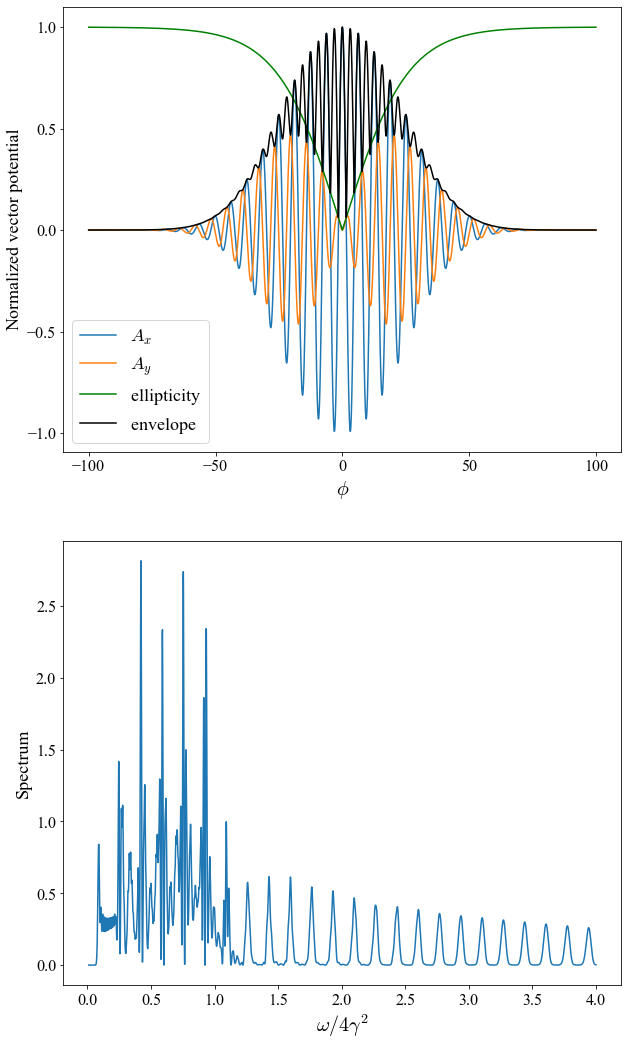
Figure 1: (Top) Vector potential and ellipticity of a polarization gated pulse for the optimal delay $\delta=\tau$. (Bottom) Corresponding backscattered spectrum. Vector potential and intensity are normalized. Laser pulse parameters: $a_{0}=3,\tau=8\pi$.

To investigate whether such comb pattern remains in the angular distribution, we calculated the spectrum dependence on the solid angle $\Omega$ and integrated it over the polar angle. We observed that for the optimal delay parameter the comb could be still seen, although the more one goes away from the axis, the more broad and messy the harmonics comb will be. For delays that are not close to optimal, results seem to repeat the on-axis case: no distinct pattern in the harmonics spectrum was noticed.

From the experimental point of view, it is especially interesting to discuss obtained results in the laboratory frame and whether a gamma comb could be detected. As it is well-known, Lorentz transforming back does not change the on-axis spectrum qualitatively (only the frequency is upshifted by $4\gamma^{2}$), therefore, the on-axis gamma comb remains. Figure 2 shows that the angular spectrum is squeezed into $1/\gamma$ cone but the pattern is still visible. In the close vicinity to the axis, one can obtain the harmonics comb for $\omega>4\gamma^{2}$ and directly measure it in experiments.

We would also like to repeat that the polarization gating technique is not aimed to avoid the ponderomotive broadening around the fundamental Compton line which could be noticed from both figures. In the electron’s rest frame the main line is broadened up to $\omega=1$ and interferes with harmonics falling into this interval, that is why only from $\omega\sim 1$ the effect shows itself.

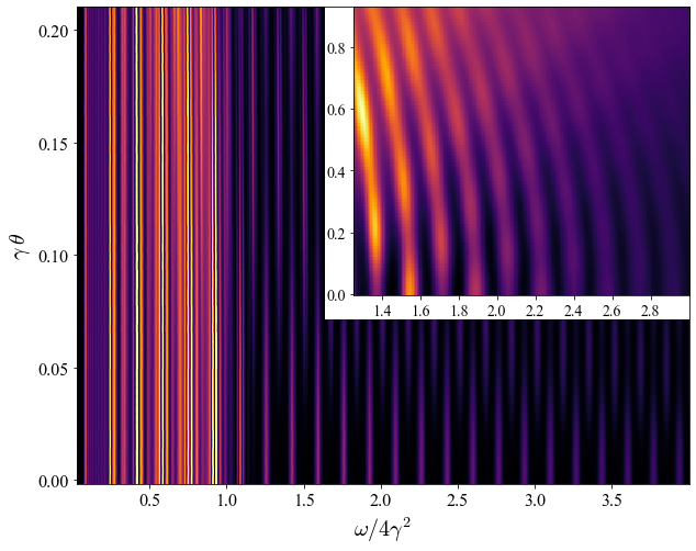
Figure 2: Radiation angular spectrum in the Lab frame for the optimal delay parameter $\delta=\tau$, $\gamma=529$. (Main) From one electron, $a_{0}=3,\tau=8\pi$. (Corner) From a realistic electron beam, $a_{0}=2,\tau=30\pi$.

Such comb has two characteristic properties: the distance between two adjacent peaks and the width of each harmonic, which could be controlled by the strength and length of the incident pulse ($a_{0}$ and $\tau$). Figure 3 shows the normalized backscattered spectrum in the gamma region of optimal PGPs for different $a_{0}=1.5,\>3$ and $\tau=6\pi,\>12\pi$. The distance between two peaks could be estimated from Eqs. (1)-(2) as $\Delta=2/(1+2a_{0}^{2}e^{-1/2})$ (the exponential factor is due to the gaussian temporal envelope) and is governed solely by $a_{0}$. Therefore, more intense laser pulses form more frequent gamma combs. As for the harmonic width, for longer laser pulses the comb is narrower (see Figure 3) as well as for more intense ones.

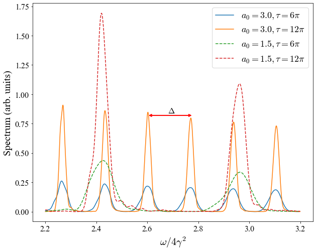
Figure 3: Normalized backscattered harmonics spectrum of an optimal polarization gated pulse for different pulse lengths: $6\pi,12\pi$; and strengths $a_{0}=1.5,3$. Red arrow shows the distance between the 31st and 33rd harmonic.

It is quite interesting to calculate how many photons are emitted into one particular harmonic. The exact photon number in the desired bandwidth $\frac{d^{2}N_{ph}}{d\omega d\Omega}=\alpha\frac{1}{\omega}\frac{d^{2}I}{d\omega d\Omega}$, where $\alpha\approx 1/137$ is the fine structure constant, could be estimated by integrating the photon spectrum over the proper collimation angle. The harmonics frequency is known from Eq. (2), and its approximate width could be numerically estimated. For instance, if we scatter a plane wave ($a_{0}=3,\tau=8\pi$) on a single electron ($\gamma=529$), integrate the differential number of photons over the collimation angle $\theta_{col}=0.2/\gamma$, then the number of photons in the 23rd harmonic in the bandwidth $\frac{\Delta\omega}{\omega}\approx 0.04$ is around $1.9\cdot 10^{-5}$. In order to estimate whether a gamma comb could be observed in the real-life experimental setup, we simulated the interaction of a non-ideal electron beam with a polarization gated pulse using the code VDSR Chen et al. (2013). The electron beam had realistic parameters: central gamma factor $\gamma=529$, normalized emittance $\epsilon_{n}\approx 0.14$ mm mrad, transverse radius $\sigma_{r}\approx 1.4\>\mu$m, angular divergence $\sigma_{\theta}\approx 0.19$ mrad, energy divergence $\approx 1\%$. The laser pulse was simulated in the paraxial approximation with $\lambda_{0}=0.8\>\mu$m and spotsize $w_{0}=24\>\mu$m. Figure 4 shows the differential number of photons in the gamma region integrated over the collimation angle $\theta_{col}=0.2/\gamma$ scattered from an electron beam ($10^{8}$ electrons represented by $4800$ macro particles). For instance, there are $\sim 10^{4}$ photons in the 11th harmonic. Due to the relatively large collimation angle and electron beam non-ideal effects, one can observe even, off-axis harmonics between the gamma comb peaks. We can see that due to the broadening caused by the beam’s angular and energy divergence Rykovanov et al. (2014), harmonics start to overlap, but nevertheless, the nearest harmonics are still distinctly seen while the highest harmonics are more blurred. The reason is that the highest harmonics are less intensive, therefore not so noticeable against the background. This particular simulation shows that the gamma comb could be observed using a compact setup employing a laser system driving both the LPA and backscattering. One should mention that the photon numbers in a single narrow bandwidth line in the polarization gating method are comparable to those in conventional Compton backscattering facilities Weller et al. (2009). This makes our proposed scheme feasible for future photo-nuclear physics experiments.

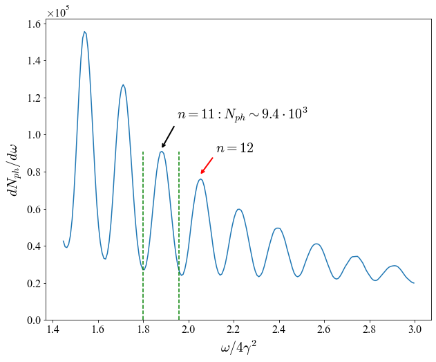
Figure 4: The differential number of photons in the gamma region scattered from a realistic electron beam ($10^{8}$ electrons represented by $4800$ macro particles, $\gamma=529$). Laser pulse parameters: $a_{0}=2,\tau=30\pi$.

In strong-field QED, nonlinear Compton scattering is described as a first-order process in the Furry picture using known solutions of the Dirac equation for the dressed electrons in the plane wave - Volkov spinor wave functions $\Psi_{p,\sigma}$ with asymptotic four-momentum $p$ and spin-polarization $\sigma$ Kharin et al. (2018). We also checked that in numerical simulations based on QED description the gamma comb is present.

Overall, we proposed a polarization gating technique - an experimentally feasible and simple method for avoiding the ponderomotive broadening (caused by temporal envelope) in the harmonics spectrum. We showed that for the optimal delay between circular pulses (which equals pulse length) one can observe a narrow bandwidth comb in the gamma region for the backscattered spectrum as well as for angular spectrum. Such an effect may arise due to the fact that we limit harmonics emission to the region around the pulse’s peak, where the harmonics emission efficiency is the highest and intensity gradients are the smallest, which significantly reduces ponderomotive broadening. One can change the laser pulse intensity and length to control how frequent and narrow the gamma comb will be. By choosing a proper collimation angle one may estimate the number of photons in a particular harmonic. We simulated the interaction of the polarization gated pulse with a realistic electron beam and showed that the gamma comb could still be observed in the real-life experimental setup. For the proof-of-principle experiments, it would make sense to perform a fully optical experiment using an LPA and a scattering laser. However, for the usage of the proposed gamma comb as a bright source, it seems to be better to use conventional accelerators due to their superior longitudinal and transverse emittance. Our proposed scheme might be useful in photo-nuclear experiments as well as nonlinear QED experiments planned at DESY (LUXE Abramowicz et al. (2021); Kämpfer and Titov (2021)) and SLAC (experiment E-320).

The authors acknowledge the usage of Skoltech CDISE supercomputer “Zhores” Zacharov et al. (2019) for obtaining the numerical results presented in this paper. S.R. would like to thank V.G. Nedorezov for fruitful discussions.

References

- Faure et al. (2004) J. Faure, Y. Glinec, A. Pukhov, S. Kiselev, S. Gordienko, E. Lefebvre, J.-P. Rousseau, F. Burgy, and V. Malka, Nature 431, 541 (2004).
- Blumenfeld et al. (2007) I. Blumenfeld, C. E. Clayton, F.-J. Decker, M. J. Hogan, C. Huang, R. Ischebeck, R. Iverson, C. Joshi, T. Katsouleas, N. Kirby, et al., Nature 445, 741 (2007).
- Nedorezov et al. (2004) V. G. Nedorezov, A. A. Turinge, and Y. M. Shatunov, UFN 174, 353 (2004).
- Geddes et al. (2015) C. G. Geddes, S. Rykovanov, N. H. Matlis, S. Steinke, J.-L. Vay, E. H. Esarey, B. Ludewigt, K. Nakamura, B. J. Quiter, C. B. Schroeder, et al., Nuclear Instruments and Methods in Physics Research Section B: Beam Interactions with Materials and Atoms 350, 116 (2015).
- Rykovanov et al. (2014) S. Rykovanov, C. Geddes, J. Vay, C. Schroeder, E. Esarey, and W. Leemans, Journal of Physics B: Atomic, Molecular and Optical Physics 47, 234013 (2014).
- Albert et al. (2011) F. Albert, S. Anderson, D. Gibson, R. Marsh, S. Wu, C. Siders, C. Barty, and F. Hartemann, Physical Review Special Topics-Accelerators and Beams 14, 050703 (2011).
- Bertozzi et al. (2008) W. Bertozzi, J. A. Caggiano, W. K. Hensley, M. S. Johnson, S. Korbly, R. Ledoux, D. P. McNabb, E. Norman, W. H. Park, and G. A. Warren, Physical Review C 78, 041601 (2008).
- Quiter et al. (2011) B. J. Quiter, B. A. Ludewigt, V. V. Mozin, C. Wilson, and S. Korbly, Nuclear Instruments and Methods in Physics Research Section B: Beam Interactions with Materials and Atoms 269, 1130 (2011).
- Carroll et al. (2003) F. E. Carroll, M. H. Mendenhall, R. H. Traeger, C. Brau, and J. W. Waters, American journal of roentgenology 181, 1197 (2003).
- Weeks et al. (1997) K. Weeks, V. Litvinenko, and J. Madey, Medical physics 24, 417 (1997).
- Quiter et al. (2008) B. Quiter, S. Prussin, B. Pohl, J. Hall, J. Trebes, G. Stone, and M.-A. Descalle, Journal of Applied Physics 103, 064910 (2008).
- Carpinelli and Serafini (2009) M. Carpinelli and L. Serafini, Nuclear Inst. and Methods in Physics Research, A 1, v (2009).
- Hartemann et al. (1996) F. Hartemann, A. Troha, N. Luhmann Jr, and Z. Toffano, Physical Review E 54, 2956 (1996).
- Hartemann and Wu (2013) F. V. Hartemann and S. S. Wu, Physical review letters 111, 044801 (2013).
- Rykovanov et al. (2016) S. Rykovanov, C. Geddes, C. Schroeder, E. Esarey, and W. Leemans, Physical Review Accelerators and Beams 19, 030701 (2016).
- Heinzl et al. (2010) T. Heinzl, D. Seipt, and B. Kämpfer, Physical Review A 81, 022125 (2010).
- Seipt and Kämpfer (2011) D. Seipt and B. Kämpfer, Physical Review A 83, 022101 (2011).
- Ghebregziabher et al. (2013) I. Ghebregziabher, B. A. Shadwick, and D. Umstadter, Physical Review Special Topics-Accelerators and Beams 16, 030705 (2013).
- Terzić et al. (2014) B. Terzić, K. Deitrick, A. S. Hofler, and G. A. Krafft, Physical Review Letters 112, 074801 (2014).
- Seipt et al. (2015) D. Seipt, S. Rykovanov, A. Surzhykov, and S. Fritzsche, Physical Review A 91, 033402 (2015).
- Terzić et al. (2016) B. Terzić, C. Reeves, and G. A. Krafft, Physical Review Accelerators and Beams 19, 044403 (2016).
- Kharin et al. (2018) V. Y. Kharin, D. Seipt, and S. G. Rykovanov, Physical review letters 120, 044802 (2018).
- Seipt et al. (2019) D. Seipt, V. Y. Kharin, and S. G. Rykovanov, Physical review letters 122, 204802 (2019).
- Rykovanov et al. (2008) S. G. Rykovanov, M. Geissler, J. Meyer-ter Vehn, and G. D. Tsakiris, New Journal of Physics 10, 025025 (2008).
- Brau (2004) C. Brau, Physical Review Special Topics-Accelerators and Beams 7, 020701 (2004).
- Kharin et al. (2016) V. Y. Kharin, D. Seipt, and S. Rykovanov, Physical Review A 93, 063801 (2016).
- Nikishov and Ritus (1964) A. Nikishov and V. Ritus, Sov. Phys. JETP 19, 529 (1964).
- Mourou et al. (2006) G. A. Mourou, T. Tajima, and S. V. Bulanov, Reviews of modern physics 78, 309 (2006).
- Di Piazza (2008) A. Di Piazza, Letters in Mathematical Physics 83, 305 (2008).
- Thomas et al. (2012) A. Thomas, C. Ridgers, S. Bulanov, B. Griffin, and S. Mangles, Physical Review X 2, 041004 (2012).
- Ruijter et al. (2018) M. Ruijter, V. Y. Kharin, and S. Rykovanov, Journal of Physics B: Atomic, Molecular and Optical Physics 51, 225701 (2018).
- Esarey et al. (1993) E. Esarey, S. K. Ride, and P. Sprangle, Physical Review E 48, 3003 (1993).
- Jackson (1999) J. D. Jackson, Classical electrodynamics (1999).
- Chen et al. (2013) M. Chen, E. Esarey, C. Geddes, C. Schroeder, G. Plateau, S. Bulanov, S. Rykovanov, and W. Leemans, Physical Review Special Topics-Accelerators and Beams 16, 030701 (2013).
- Weller et al. (2009) H. R. Weller, M. W. Ahmed, H. Gao, W. Tornow, Y. K. Wu, M. Gai, and R. Miskimen, Progress in Particle and Nuclear Physics 62, 257 (2009).
- Abramowicz et al. (2021) H. Abramowicz, U. H. Acosta, M. Altarelli, R. Assmann, Z. Bai, T. Behnke, Y. Benhammou, T. Blackburn, S. Boogert, O. Borysov, et al., arXiv preprint arXiv:2102.02032 (2021).
- Kämpfer and Titov (2021) B. Kämpfer and A. Titov, Physical Review A 103, 033101 (2021).
- Zacharov et al. (2019) I. Zacharov, R. Arslanov, M. Gunin, D. Stefonishin, A. Bykov, S. Pavlov, O. Panarin, A. Maliutin, S. Rykovanov, and M. Fedorov, Open Engineering 9, 512 (2019).