Abstract

We argue that under certain assumptions the quantum break time approach and the trans-Planckian censorship conjecture both lead to de Sitter swampland constraints of the same functional form. It is a well known fact that the quantum energy-momentum tensor in the Bunch-Davies vacuum computed in the static patch of dS breaks some of the isometries. Proposing that this is a manifestation of quantum breaking of dS, we analyze some of its consequences. In particular, this leads to a thermal matter component that can be generalized to string theory in an obvious way. Imposing a censorship of quantum breaking, we recover the no eternal inflation bound in the low temperature regime, while the stronger bound from the dS swampland conjecture follows under a few reasonable assumptions about the still mysterious, presumably topological, high-temperature regime of string theory.

1 Introduction

The de Sitter (dS) space-time is one of the most studied solutions of Einstein’s equations, partially because of its value for cosmological considerations. Its possible instability has been a matter of great interest already since the 80s [1, 2] as it could provide an explanation for the cosmological constant problem. By now there exist indications that quantum gravity does not admit long-lived de Sitter solutions. The most developed candidate for a theory of quantum gravity, namely string theory, does not yet feature a fully controlled meta-stable dS minimum that is beyond any doubt. The KKLT construction [3], which gives a dS minimum as the result of a non-trivial three step procedure, still lies in the center of an on-going debate regarding its viability. Several lines of reasoning can lead to conjectures and bounds which qualitatively forbid long-lived dS vacua, yet their mutual interrelations and respective regimes of validity are not clear. The aim of the present paper is to put some of these conjectures into perspective, and to do so, let us start by briefly reviewing the relevant bounds and their origins.

Swampland bounds on the scalar potential

In the context of the string swampland, put forward in [4] and more recently reviewed in [5, 6, 7], the difficulty in constructing dS solutions with a bona fide ten-dimensional uplift is thought to be no coincidence. In particular, it points towards the idea of de Sitter not being allowed in string theory at all [8, 9]. In [10] the quantitative dS swampland conjecture was proposed, according to which the effective four-dimensional scalar potential $V$ always satisfies

$$\begin{split}M_{\rm pl}|V^{\prime}|\geq c\cdot V\,,\end{split}$$ (1.1)

where $c$ is an ${O}(1)$ positive number and in particular independent of $V$, though possibly $n$-dependent when considering $n$ space-time dimensions. In [11] the observational consequences of such a bound were discussed.

Clearly, this conjecture is trivially satisfied for extrema of the potential whenever $V<0$, while it forbids dS vacua with $V>0$. It is worth noting that for $V>0$ the dS swampland bound can alternatively be expressed as a lower bound for the value of the slow-roll parameter $\epsilon$. Such a bound, in a much more restricted setup, was already computed in [12] using a simple scaling argument, and was later generalized in [10].

Soon it became clear that the conjecture should be slightly relaxed to allow for certain dS maxima/saddle points [13, 14]. The refined dS conjecture [15] supplemented the initial conjecture with the alternative clause:

$$\begin{split}M_{\rm pl}^{2}|V^{\prime\prime}|\geq c^{\prime}\cdot V\,,\end{split}$$ (1.2)

where $c^{\prime}$ is once again an ${O}(1)$ constant. The same generalization of the dS conjecture was already proposed in [16] in terms of the two slow-roll parameters $\epsilon,\eta$.

While the dS swampland conjecture is mostly motivated by string tree-level examples, a conjecture with a more direct physical motivation was proposed in [17]. This is the trans-Planckian censorship conjecture (TCC), which states that sub-Planckian fluctuations in an expanding quasi dS space should not become classical. Applying this conjecture to scalar fields and focusing only on positive potentials, one gets bounds very similar to the dS conjecture. In particular, in the asymptotic limit of the field space TCC assumes the form

$$\begin{split}M_{\rm pl}^{\frac{n-2}{2}}\left(\frac{|V^{\prime}|}{V}\right)_{\infty}\geq\frac{2}{\sqrt{(n-1)(n-2)}}\,.\end{split}$$ (1.3)

This TCC limiting case is of the same form as the dS conjecture, while also providing an explicit prediction for the value of $c$. If we do not invoke this asymptotic limit, the TCC is in general weaker than the dS conjecture, in the sense that sufficiently short-lived dS vacua are permitted. The physical motivation of the TCC has been debated [18, 19] recently. Here we do not intend to enter this discussion, but throughout this paper we rather consider TCC as a working assumption from which other swampland constraints can be inferred.

Another proposal which restricts the scalar potential and its derivatives is the “no eternal inflation” principle. In [20] necessary conditions for (no) eternal inflation were inferred by solving the Fokker-Planck equation for stochastic inflation. For several types of potentials, the no eternal inflation bounds exhibited remarkable similarities to several formulations of the (refined) dS conjecture. This hinted at a no eternal inflation principle as a possible deeper reason behind the swampland conjectures. In the present paper we will mostly be concerned with slowly-rolling scalar fields, so we start with the case of a four-dimensional linear potential. There, the no eternal inflation principle imposes the bound

$$\begin{split}M_{\rm pl}\frac{|V^{\prime}|}{V}>\frac{\sqrt{2}}{2\pi}\bigg{(}\frac{V}{M_{\rm pl}^{4}}\bigg{)}^{1/2}\,.\end{split}$$ (1.4)

This is remarkably similar to the dS conjecture (1.1), but now the right-hand side is still $V$-dependent, relaxing the bound significantly for small and positive $V$. Let us note that conditions necessary for eternal inflation, possibly differing in the ${O}(1)$ constant, were already obtained in [21, 22, 23]. The compatibility of eternal inflation with the dS swampland conjecture has also been studied in [24].

Moreover, the bound (1.4) was generalized to $n$ dimensions in [25], where it assumes the form

$$\begin{split}M_{\rm pl}^{\frac{n-2}{2}}\frac{|V^{\prime}|}{V}>c^{\prime\prime}\cdot\bigg{(}\frac{V}{M_{\rm pl}^{n}}\bigg{)}^{\frac{n-2}{4}},\end{split}$$ (1.5)

with $c^{\prime\prime}$ again an ${O}(1)$ positive constant. In the following, we will refer to any bound of the form $|V^{\prime}|/V>{c}\cdot V^{\frac{n-2}{4}}$ as a no eternal inflation bound, irrespective of the precise value of this positive constant ${c}$. Moreover, we are setting the reduced Planck mass to one, unless explicitly stated.

One should keep in mind that different types of potentials result in different bounds. For a four-dimensional quadratic hilltop potential, the no eternal inflation principle translates to the bound

$$\begin{split}M_{\rm pl}^{2}\frac{|V^{\prime\prime}|}{V}>3\,.\end{split}$$ (1.6)

Provided $c^{\prime}>3$, this is compatible with the refined dS conjecture (1.2). Similar bounds, up to ${O}(1)$ factors, for eternal hilltop inflation were also derived in [26, 27].

An intricate relation between the TCC and the no eternal inflation principle was recently revealed in [25]. There, a sequence of short-lived dS bubbles, transitioning from one to the next through non-perturbative membrane nucleation, was described in terms of a dual low-energy effective scalar potential. Imposing TCC was sufficient to find the allowed region in the parameter space, which turned out to marginally exclude eternal inflation, thus leading to a bound of the form $|V^{\prime}|>c\cdot V^{3/2}$.

Quantum breaking of de Sitter and relation to swampland

The idea of having an upper bound on the life-time of de Sitter is not new. In a different line of research [28, 29, 30], a corpuscular picture of de Sitter space was proposed, which allowed to capture quantum effects invisible to the usual semiclassical treatment of gravity. Those effects are found to induce a finite life-time for classical dS solutions, the so-called quantum break time. More specifically, the dS solution is viewed as a coherent state of gravitons over Minkowski space. Decoherence of this state, i.e. quantum scattering of gravitons from the coherent state, leads then to the quantum break time, that is the finite time-scale after which the mean field description ceases being valid. A general expression for this life-time was given by $t_{Q}\sim t_{\rm cl}/\alpha$, where $t_{\rm cl}$ denotes the characteristic time scale of the system and $\alpha$ the quantum interaction strength of the constituents. For a four-dimensional inflating phase in pure Einstein gravity, the first parameter is the Hubble time $t_{\rm cl}=H^{-1}$ and the second one $\alpha=H^{2}/M_{\rm pl}^{2}$, i.e. an effective strength of graviton scattering for the characteristic momentum transfer $H$. Thus, the quantum break time becomes $t_{q}\sim M_{\rm pl}^{2}/H^{3}$.

In view of the stringy swampland conjectures, this picture was extended in [32, 33] by suggesting that quantum breaking should not occur. The theory must censor it by providing a (classical) mechanism that leads to a faster decay of de Sitter. Such a behavior is for instance exhibited by a sufficiently fast rolling scalar field with slow-roll parameter $\epsilon$ and the associated classical time-scale $t_{\rm cl}\sim 1/(\epsilon H)$. Requiring $t_{\rm cl}\lesssim t_{q}$ leads to the following bound on the gradient of the potential

$$\begin{split}M_{\rm pl}\frac{|V^{\prime}|}{V}\gtrsim c\cdot\bigg{(}{\frac{V}{M^{4}_{\rm pl}}}\bigg{)}^{\frac{1}{2}},\ \end{split}$$ (1.7)

which takes the same form as the no eternal inflation bound and is therefore weaker than the dS swampland conjecture. The only way to get the stronger bound of the dS conjecture would be a scaling $t_{q}\sim H^{-1}$.

The present work examines whether also the dS swampland bound (1.1) can be derived in a similar fashion as a quantum breaking bound. Since the bound (1.7) is derived using a quantum description of classical gravity, it is natural to suspect that the answer is related to a generalization to a more complete quantum gravitational theory like string theory, loop quantum gravity or any of the possible candidates. It has already been pointed out in [32, 33] that in perturbative string theory the bound might get stronger. One proposal was that in string theory the natural estimate for the interaction strength is the string coupling constant $\alpha=g_{s}^{2}$. This leads indeed to the required $t_{Q}\sim H^{-1}$ scaling but would also imply a factor of $g_{s}^{2}$ in the dS swampland bound (1.1). Notice that such a factor is not present in the TCC bound (1.3).

It would be interesting to generalize the approach [28, 29, 30] to string theory with its additional ingredients like higher-form fields and massive excitations. Here, we will follow a different route that we find easier to generalize to string theory. Recall that in the corpuscular picture of [30], the decoherence is caused by the scattering of gravitons that comprise the coherent state and thus can be considered as the backreaction of the quantum state on the classical geometry.

This is reminiscent of what was discussed in the past [37, 38, 39], when in a semiclassical approach people computed the expectation value of the energy-momentum tensor $\langle T_{\mu\nu}\rangle_{\rm BD}$ of a scalar field propagating on a curved classical dS background geometry. Using Friedmann-Lemaître-Robertson Walker (FLRW) coordinates one could define the thermal Bunch-Davies vacuum that led to an energy-momentum tensor that preserved all the dS isometries. Considering the backreaction of this quantum contribution on the right-hand side of the Einstein equation only gives rise to a small redefinition of the cosmological constant. On the other hand, it is known that performing the same computation in the static dS patch leads to a qualitatively different result. In this case $\langle T_{\mu\nu}\rangle_{\rm BD}$ diverges on the dS horizon and does not preserve the isometries but instead contains a (matter-like) thermal component with an equation of state parameter $\omega\neq-1$. For instance, for the 4D conformal case, one finds a thermal, time-independent energy-momentum tensor with an equation of state $p=\rho/3$ and a temperature equal to the Gibbons-Hawking temperature $T=H/(2\pi)$ of the dS horizon [40].

If one includes this contribution in the Einstein equation, it will cause a deviation from the initial dS geometry. We will see that the relevant time scale for this change is the same as the quantum breaking time of [30]. The puzzle of the prediction of qualitatively different evolutions of dS in FLRW and the static patch is resolved by censoring quantum breaking, i.e. by conjecturing that the full theory of quantum gravity even classically will not admit eternal dS solutions but at best quasi dS ones, where e.g. the scalar field is still evolving like in quintessence models.

Thus, in this paper we will work under the assumption that though diverging at the horizon, the quantum energy-momentum tensor in the static patch gives a physically reasonable quantity, at least in the vicinity of the center of the patch, whose backreaction causes quantum breaking. In the following we will call this approach the “quantum backreaction approach”.

A pictorial overview and outline

Let us summarize what we have mentioned up to now in a pictorial way in figure 1. There we present only the bounds on $|V^{\prime}|/V$ for a four-dimensional potential, but during the course of the paper we will also consider the bounds on $|V^{\prime\prime}|/V$.

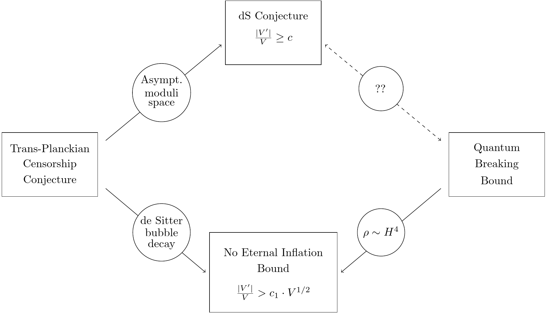
Figure 1: Schematic depiction of bounds for $|V^{\prime}|/V$ for a (positive) scalar potential $V$ in 4D and their origin in terms of swampland conjectures or avoidance of the quantum breaking. $c,c_{1}$ are positive ${O}(1)$ constants.

We see that as far as the swampland program is concerned, de Sitter vacua are short-lived if at all allowed. It is by now well known that the swampland conjectures [4, 44, 45, 46, 10, 15, 47, 48] are not independent but form a tightly-knit web, with many connections between its nodes. TCC is postulated to be one of the central nodes [54], and in this paper we “zoom in” on only two of its derivative conjectures. This can be seen on the left-hand side of the figure, as TCC can lead to both the dS swampland conjecture and the no eternal inflation bound. The former case arises when considering an asymptotic limit in the field space, while the latter bound is reached through the more complicated dS bubble cascade decay. On the right-hand side of the figure we have the quantum breaking approach. Requiring that dS decays fast enough to avoid reaching the quantum break time, via both the usual quantum corpuscular description and the quantum backreaction approach, leads to the less strict $|V^{\prime}|/V>c_{1}\cdot V^{1/2}$ no eternal inflation bound.

Clearly in this picture there is one link missing that would connect the censoring of quantum breaking directly to the dS conjecture. As already suggested in [32, 33] this link should be related to inherently quantum gravitational effects. Our analysis will eventually lead us to the very intriguing suspicion that it is the high temperature regime of quantum gravity that provides the missing link. There is evidence not only from string theory, but also from other approaches to quantum gravity (see [55, 56]) that in this regime the number of degrees of freedom is reduced and effectively the theory becomes two-dimensional. A full description of this phase is yet to be provided, but there are indications that it might be related to a topological gravity theory. Note that this proposal is also the basis for the recent idea of Agrawal, Gukov, Obied, Vafa [57] that the early history of the universe is not described by inflation but by such a topological gravity theory [58].

In the present paper we intend to put more flesh on this idea and make it concrete in the framework of the quantum backreaction approach. Since in the course of our arguments we will employ various conceptually different techniques, we have made an attempt to provide a self-contained presentation of the relevant material.

The paper is organized as follows: In section 2 we explain the quantum backreaction approach to quantum breaking in some detail by first reviewing known results from the literature and recalling that some of them are already fixed by the conformal anomaly. Then we generalize the results for the energy-momentum tensor in the static patch to higher dimensions and non-conformal scalars. As we will show, this includes a time-independent, thermal matter component, which gives rise to an evolution of the Hubble parameter, leading to a finite quantum break time. Moreover, by discussing a non-conformal, massive scalar in 4D as an enlightening example, we will see that to a good approximation the energy-density is given by the familiar flat space result. The only deviation comes from a kind of a resonant behavior when the Compton wavelength of the massive scalar is equal to the size of the dS space. The similarity to the just mentioned flat space thermal contribution will be directly generalized to string theory, thus connecting to well known approaches to compute thermal one-loop partition functions in string theory.

In section 3 we recall the thermodynamics of strings at finite temperature, focusing on the computation of the thermal partition function and the related free energy, energy density and pressure. The salient new feature appearing in string theory is the existence of the so-called Hagedorn temperature $T_{H}$, where due to the condensation of a stringy winding mode, the system is supposed to experience a first order phase transition. Not much is known about this new phase of strings, but the seminal work of Atick-Witten [59] suggested that the temperature dependence of the energy density in any dimension is quadratic, hence indicating a radical reduction of the number of degrees of freedom. Such a reduction was previously also observed in high energy scattering of strings [60].

In section 4 we study the behavior of the aforementioned quantities in the low and the high temperature regimes. In the former, methods from perturbative string theory are under control whereas for the latter, we have to rely on (naive) extrapolations and well-motivated guesswork. Estimating the quantum break time for these two distinct phases, we find that the low temperature regime leads to a bound on $|V^{\prime}|/V$ of the no eternal inflation principle type, while the high temperature regime produces the dS swampland conjecture bound. Therefore, from this perspective there seems to be a relationship between the dS swampland conjecture and the still mysterious high temperature phase of string theory.

2 Quantum breaking of dS from backreaction

We start this section by reviewing the computation of the (BD) vacuum expectation value of the energy-momentum tensor for a quantized conformal scalar field in a classical dS space-time. We highlight the difference between the results in FLRW coordinates and in the static patch. Then we provide a systematic approach to compute the latter in the center of the static patch also for the non-conformal case. All this will lead us to the conjecture that quantum backreaction is a manifestation of quantum breaking. We will also comment on the similarity to Rindler space which, if taken seriously, will lead to the conjecture that eternal flat Minkowski space is not a solution of (non-supersymmetric) quantum gravity, either.

2.1 Brief review of the conformal case

To make our point, let us first consider the simplest case of a conformally coupled scalar field $\Phi$ in $n$-dimensional de Sitter space. For dS space we consider two different coordinate systems. First, we have the Friedmann-Lemaître-Robertson-Walker (FLRW) coordinates, whose line element is given by

$$\begin{split}ds^{2}=-dt^{2}+a^{2}(t)d\boldsymbol{x}^{2}=-dt^{2}+e^{2Ht}d\boldsymbol{x}^{2}\,,\end{split}$$ (2.1)

with $t\in[-\infty,\infty]$ and the spatial coordinates $x^{i}\in[-\infty,\infty]$. Introducing the conformal time $\eta$ via $d\eta=dt/a(t)$, this can be expressed as

$$\begin{split}ds^{2}={\frac{1}{H^{2}\eta^{2}}}\left(-d\eta^{2}+d\boldsymbol{x}^{2}\right)\end{split}$$ (2.2)

which makes it evident that the metric is conformally flat. The FLRW coordinate system is the most common choice for quantizing a scalar field in de Sitter space. There exists a family of vacua extending over the whole FLRW patch which respect the isometries of dS, the so-called $\alpha$-vacua [1, 61]. A special case among them is the famous Chernikov-Tagirov or Bunch-Davies (BD) vacuum [62, 63], which is thermal and leads to a scale-invariant power spectrum consistent with CMB fluctuations. For further information on dS coordinate systems and the BD vacuum we refer to some standard references [64, 65, 66].

The de Sitter horizon is not explicitly visible in the FLRW patch. To make it manifest it is more appropriate to use the metric in the static coordinate system

$$\begin{split}ds^{2}=-(1-H^{2}r^{2})\,d\tau^{2}+\frac{dr^{2}}{1-H^{2}r^{2}}+r^{2}d\Omega^{2}_{n-2}\,.\end{split}$$ (2.3)

Here the metric components are time-independent and there is a coordinate singularity at the horizon $r_{h}=H^{-1}$. While the FLRW patch covers half of the dS manifold, including a region beyond the horizon, this does not hold for the static case. One has to distinguish the regions inside $0\leq r\leq H^{-1}$ (region A) and outside $r\geq H^{-1}$ of the horizon (region B), where for the latter case $\tau$ becomes spacelike and $r$ timelike (and the metric is no longer strictly speaking “static”). The FLRW patch is then covered by the two static patches. Let us note that in the two-dimensional case a further third static patch (beyond the horizon) exists.

The action for a conformally coupled scalar on de Sitter space reads

$$\begin{split}S_{m}=-\int d^{n}x\sqrt{-g}\left[\frac{1}{2}\partial_{\mu}\Phi\,\partial^{\mu}\Phi+\frac{\xi}{2}R\,\Phi^{2}\right],\end{split}$$ (2.4)

where $\xi=\frac{(n-2)}{4(n-1)}$ is the conformal coupling and $R=n(n-1)H^{2}$ denotes the Ricci scalar of $dS_{n}$. The object of interest is the vacuum expectation value $\langle T_{\mu\nu}\rangle$ of the energy-momentum tensor

$$\begin{split}T_{\mu\nu}=\partial_{\mu}\Phi\partial_{\nu}\Phi-{1\over 2}g_{\mu\nu}\partial^{\rho}\Phi\partial_{\rho}\Phi+\xi\Big{(}G_{\mu\nu}-\nabla_{\mu}\nabla_{\nu}+g_{\mu\nu}\Box\Big{)}\Phi^{2}\end{split}$$ (2.5)

in the Bunch-Davies vacuum. Here $G_{\mu\nu}$ denotes the Einstein-tensor. For clarity let us now focus on the two-dimensional case, where one can employ results from 2D conformal field theory.

Conformal scalar in 2D

Since we are dealing with a 2D conformal field theory, it is appropriate to introduce light-cone coordinates. In the FLRW patch these are given by

$$\begin{split}U=\eta-x\,,\quad V=\eta+x\ \Rightarrow\ ds^{2}=-{\textstyle{4\over H^{2}(U+V)^{2}}}\,dU\,dV\,,\end{split}$$ (2.6)

whereas in static coordinates one can introduce

$$\begin{split}u=\tau-r^{*}\,,\quad v=\tau+r^{*}\ \Rightarrow\ ds^{2}=-{\textstyle{1\over\cosh^{2}\left({H\over 2}(v-u)\right)}}\,du\,dv\end{split}$$ (2.7)

with $r={1\over H}\tanh(Hr^{*})$. These two metrics are conformally equivalent via the corresponding conformal transformation inside the horizon

$$\begin{split}U=-{1\over H}e^{-Hu}\,,\qquad V=-{1\over H}e^{-Hv}\,,\end{split}$$ (2.8)

while similar expressions exist for the remaining patches[43]. In FLRW coordinates the vacuum expectation value of the energy-momentum in the Bunch-Davies vacuum can be computed as

$$\langle T^{\rm div}_{UU}\rangle_{BD}=\langle T^{\rm div}_{VV}\rangle_{BD}={1\over 4\pi}\int_{0}^{\infty}kdk\,,\qquad\langle T^{\rm div}_{UV}\rangle_{BD}=0$$ (2.9)

which is of course divergent and needs to be regularized. Applying adiabatic regularization [68, 69] gives the counterterms

$$\delta T^{BD}_{UU}=\delta T^{BD}_{VV}={1\over 4\pi}\int_{0}^{\infty}kdk\,,\qquad\delta T^{BD}_{UV}={H^{2}\over 24\pi}g_{UV}$$ (2.10)

leading to the renormalized energy-momentum tensor

$$\langle T^{\rm ren,FLRW}_{UU}\rangle_{BD}=\langle T^{\rm ren,FLRW}_{VV}\rangle_{BD}=0\,,\qquad\langle T^{\rm ren,FLRW}_{UV}\rangle_{BD}=-{H^{2}\over 24\pi}g_{UV}\,.$$ (2.11)

Note that the off-diagonal term is dictated by the general form of the 2D conformal anomaly $\langle T^{\mu}_{\mu}\rangle=-{c\over 24\pi}R$. Moreover, since $\langle T_{\mu\nu}\rangle\sim g_{\mu\nu}$ the energy-momentum tensor preserves the dS isometries and is covariantly conserved, i.e. $\nabla^{\mu}\langle T_{\mu\nu}\rangle=0$.

Next, we want to compute the quantum energy-momentum tensor in the static patch. Since the static coordinates are related to the FLRW ones via a conformal transformation, we can employ the anomalous transformation law of the energy-momentum tensor, which in general reads

$$\left({\partial U\over\partial u}\right)^{2}T_{UU}(U)=T_{uu}(u)+{c\over 24\pi}\{U,u\}$$ (2.12)

with $\{U,u\}$ denoting the Schwarzian derivative and an analogous relation for the remaining light-cone coordinates $V$ and $v$. Here the “unusual” plus sign in the right-hand side is due to the Lorentzian signature. In this way we can derive

$$\langle T^{\rm ren,stat}_{uu}\rangle_{BD}=\langle T^{\rm ren,stat}_{vv}\rangle_{BD}={H^{2}\over 48\pi}\,,\qquad\langle T^{\rm ren,stat}_{uv}\rangle_{BD}=-{H^{2}\over 24\pi}g_{uv}\,.$$ (2.13)

which still is covariantly conserved. Note that due to the non-vanishing conformal anomaly it is inevitable that the final result is not proportional to the metric. As we will see later, this is a general behavior of the VEV of the energy-momentum tensor in the static patch. Therefore, this energy-momentum tensor is not behaving like a cosmological constant but has a component that contributes like radiation with the 2D equation of state $p=\rho$.

As will further be discussed in the next section, one can derive this result also directly by quantizing the scalar field in the static patch. After deriving the properly normalized solutions in regions A and B (inside/outside of the horizon), it is possible to construct the two continuous linear combinations $\Phi_{A}+\gamma(\Phi_{B})^{*}$ and $\gamma(\Phi_{A})^{*}+\Phi_{B}$, where $\gamma=\exp(2\pi k/H)$ has the form of a thermal factor for the Gibbons-Hawking temperature $T=H/(2\pi)$. From these combinations, the Bunch-Davies vacuum state can be expressed as the entangled so-called thermo-field double state over the two regions [70]. For a local observable inside the horizon, one can trace over region B resulting in a reduced (thermal) density matrix $\hat{\rho}$ so that the VEV of the energy-momentum tensor in region A can be computed via $\langle{T_{A}}\rangle={\rm tr}(\hat{\rho}\,{T_{A}})$.

In the conformal 2D case, one finds the divergent result

$$\begin{split}&\langle T^{\rm div}_{uu}\rangle_{BD}=\langle T^{\rm div}_{vv}\rangle_{BD}={1\over 4\pi}\int_{0}^{\infty}dk\,k\Big{(}1+{2\over e^{2\pi k/H}-1}\Big{)}\,,\\ &\langle T^{\rm div}_{uv}\rangle_{BD}=0.\end{split}$$ (2.14)

Next the issue of regularization arises. Here we cannot employ adiabatic regularization which is taylor-made for fields slowly varying with time. It goes beyond the scope of this paper to develop a consistent theory of regularization in the static patch, but we can make an important observation that will be sufficient for our purposes.

The divergent piece in (LABEL:staticdivT) comes from the zero-point energy and can be cancelled by using normal ordering among the modes. By doing this, one finds that the remaining flat space integral over the Bose-Einstein distribution indeed gives $H^{2}/(48\pi)$, consistent with (2.13). As is obvious from the conformal anomaly, there must also be an off-diagonal counterterm $\delta T^{BD}_{uv}$ which however is proportional to the metric. Therefore, in this paper we work under the following well-motivated mild assumption.

Assumption 1: A non-trivial matter contribution $\langle T^{\rm ren}_{\mu\nu}\rangle_{\rm M}$ in the static patch can be detected by computing the initially divergent vacuum expectation value of the energy-momentum tensor using the thermal reduced density matrix and then regularize it by normal ordering.

This in particular means that the other counterterms do not change the fully renormalized energy-momentum tensor such that eventually it preserves the dS isometries. Note that the so obtained energy density is time-independent so that the observer in the static patch would attribute a temperature $T=H/(2\pi)$ to the horizon that leads to a permanent inflow of Hawking radiation that is compensated by the dilution and redshifting of the inflating dS space.

Transforming this result to the local coordinates $(\tau,r)$ one can write

$$\begin{split}\langle T^{\mu}{}_{\nu}\rangle&=\langle T^{\mu}{}_{\nu}\rangle_{\rm M}+\langle T^{\mu}{}_{\nu}\rangle_{\rm CC}\\ &={H^{2}\over 24\pi(1-H^{2}r^{2})}{\rm diag}(-1,1)-{H^{2}\over 24\pi}g^{\mu}{}_{\nu}\end{split}$$ (2.15)

where we have indicated the two contributions with equation of state parameters $\omega_{M}=1$ and $\omega_{CC}=-1$. This form is often encountered in the early literature and reveals the appearance of a singularity at the horizon.

Similar computations have been performed for conformal scalar fields propagating on higher dimensional de Sitter spaces. The behavior found in 2D persists. For instance in 4D we recall the textbook result from [64]

$$\begin{split}\langle T^{\mu}{}_{\nu}\rangle={H^{4}\over 480\pi^{2}(1-H^{2}r^{2})^{2}}{\rm diag}\big{(}-1,{\textstyle{1\over 3},{1\over 3},{1\over 3}}\big{)}+{H^{4}\over 960\pi^{2}}g^{\mu}{}_{\nu}\end{split}$$ (2.16)

where in the first term one also gets a flat space thermal integral

$$\begin{split}\int_{0}^{\infty}{d^{3}k\over(2\pi)^{3}}{k\over e^{2\pi k/H}-1}=\int_{0}^{\infty}{dk\over 2\pi^{2}}{k^{3}\over e^{2\pi k/H}-1}={H^{4}\over 480\pi^{2}}\,.\end{split}$$ (2.17)

This energy-momentum tensor is still time-independent, covariantly conserved and contains a contribution with the equation of state of radiation $p=\rho/3$.

Remarks

Let us finish this section with two remarks.

• The obtained energy-momentum tensors are closely related to similar results for Rindler space (see e.g. [38, 71, 72, 73]). As shown in [38, 72], the FLRW patch of dS is in the same conformal equivalence class as flat Minkowski space, whereas the static patch of dS is in the same class as the Rindler wedge. In particular, a conformal scalar on the Rindler wedge also gives rise to a contribution to $\langle T_{\mu\nu}\rangle$ with an equation of state of radiation.

• Using the results from the next section, we can also compute the energy-momentum tensor for a scalar in three-dimensional dS space. At the center of the static patch we obtain before regularization

  $$\begin{split}\langle T^{\mu}{}_{\nu}\rangle_{r=0}=\int{d^{2}k\over(2\pi)^{2}}k\tanh({\textstyle{\pi k\over H}})\left({1\over 2}+{1\over e^{2\pi k/H}-1}\right){\rm diag}\big{(}-1,{\textstyle{1\over 2},{1\over 2}}\big{)}\end{split}$$ (2.18)

  where the extra factor $\tanh(\pi k/H)$ arises from the normalization (2.43) of the 3D wave function. It has the effect of introducing an extra suppression of the IR modes $k\ll H$. If we now regularize the integral by subtracting the zero-point contribution $1/2$ we can write

  $$\begin{split}\langle T^{\mu}{}_{\nu}\rangle_{r=0}&=\int{d^{2}k\over(2\pi)^{2}}{k\over e^{2\pi k/H}+1}{\rm diag}\big{(}-1,{\textstyle{1\over 2},{1\over 2}}\big{)}\\ &={3\zeta(3)\over 32\pi^{4}}H^{3}{\rm diag}\big{(}-1,{\textstyle{1\over 2},{1\over 2}}\big{)}\end{split}$$ (2.19)

  which intriguingly looks like the thermal expression for a free gas of fermions. This behavior persists in all odd dimensions. We cannot offer an intuitive understanding of this boson-fermion flip but note that for the quantum theory on dS differences between even and odd dimensions have already been observed e.g. in [74, 75]. Note that the integrated result still shows the expected $H^{3}$ scaling. With respect to our first remark, we have also checked that the generalization of the 4D result for Rindler space from [76] to 3D leads to the same additional $\tanh(\pi k/H)$ factor.

2.2 Proposal: Quantum Breaking

The question is what do the results reviewed in the previous subsection tell us about quantum gravity. Clearly, this was just a semiclassical analysis where a scalar field was quantized on a classical curved manifold. The metric itself was not a quantum object. The natural next step would be to include the computed quantum $\langle T_{\mu\nu}\rangle$ on the right-hand side of the Einstein equation and consider its backreaction.

As we have seen, while $\langle T^{\rm ren}_{\mu\nu}\rangle$ is still covariantly conserved, it is not transforming as a tensor under general diffeomorphisms. The latter was evident in the 2D conformal case, where it could be related to the well known 2D conformal anomaly. Thus, something is at odds here, as roughly speaking general diffeomorphisms play different roles for the left and the right-hand side of the Einstein equation:

• In general relativity general covariance is the local symmetry principle and is not expected to be broken by quantum effects.

• In the semi-classical conformal field theory, some of these diffeomorphisms are part of the global conformal symmetry, that can receive an anomaly.

Thus, whether including the backreaction is a reasonable thing to do is a matter of debate, as was expressed in the following statement from the standard textbook ’Quantum Fields in Curved Space’ by N.D. Birrell and P.C.W. Davies, Cambridge Univ. Press 1982 [64]:

’When, if ever, will the ’back-reaction’ (i.e. gravitational dynamics modified by gravitationally induced $\langle T_{\mu\nu}\rangle$) be approximately determined by $T^{\rm ren}_{\mu\nu}$ computed at the one-loop level? Misgivings about these issues have been expressed by a number of authors. Many of them might be resolved if a full theory of quantum gravity were available, to which one could claim that the semiclassical theory is some sort of approximation.’

Our point of view is that, since string theory is a theory of quantum gravity, its latest developments, in particular the swampland program, might shed some new light on this long-standing problem. Let us first look at the BD vacuum in FLRW coordinates. We have seen that in $n$ dimensions $\langle T^{\rm ren}_{\mu\nu}\rangle\sim g_{\mu\nu}H^{n}$ so it contributes on the right-hand side of the Einstein equation like the cosmological constant

$$\begin{split}R_{\mu\nu}-{1\over 2}g_{\mu\nu}R=\Lambda^{\rm cl}g_{\mu\nu}+8\pi G\,\langle T^{\rm ren}_{\mu\nu}\rangle_{\rm CC}\,\end{split}$$ (2.20)

(in the remainder of this section we set the reduced Planck scale to one, i.e. $(8\pi G)^{-1}=M_{\rm pl}^{n-2}=1$. In FLRW coordinates this leads to the single slightly perturbed Friedmann equation

$$\begin{split}{{(n-1)(n-2)\over 2}}H^{2}&=\Lambda^{\rm cl}+\kappa H^{n}\end{split}$$ (2.21)

which for $n>2$ and sub-Planckian energy scales just induces a small shift of $H$ from its initial value. Therefore, an observer in the FLRW patch would not see any dramatic change, as dS space would still be a consistent solution to the backreacted Einstein equation.

However, for an observer in the center of their static patch the backreaction would be much more substantial due to the radiation-like component in $T^{\rm ren}_{\mu\nu}$

$$\begin{split}R_{\mu\nu}-{1\over 2}g_{\mu\nu}R=\Lambda^{\rm cl}g_{\mu\nu}+\langle T^{\rm ren}_{\mu\nu}\rangle_{\rm CC}+\langle T^{\rm ren}_{\mu\nu}\rangle_{\rm M}\,.\end{split}$$ (2.22)

In this case, static de Sitter would no longer be a consistent solution of the backreacted Einstein equation. The additional component would cause $H$ to change with time, leading at best to a quasi dS space. However, this seems to be quite a paradoxical situation: observers in different patches would predict qualitatively different time evolution of space-time.

One way to resolve this is to say that the quantum energy-momentum tensor $\langle T^{\rm ren}_{\mu\nu}\rangle$ in the static patch is physically not reasonable, as it for instance features a singularity at the dS horizon and should therefore better not be included on the right-hand side of the Einstein equation.

However, in view of the recent swampland conjectures a different possibility is conceivable. In order to resolve the paradoxical situation, there should better not exist a static dS solution in quantum gravity in the first place. Thus, the best one can hope for is a quasi dS solution, with for instance a rolling quintessence field involved. In other words, there should necessarily always exist a non-vanishing classical contribution $T^{\rm cl}_{\mu\nu}(\Phi)$ of the form (2.5), induced by a gradient of $\Phi$, on the right-hand side of the Einstein equation. Hence, we can group the contributions on the right-hand side as follows

$$\begin{split}R_{\mu\nu}-{1\over 2}g_{\mu\nu}R=\Big{(}\Lambda g_{\mu\nu}+\langle T^{\rm ren}_{\mu\nu}\rangle_{\rm CC}\Big{)}+\Big{(}T^{\rm cl}_{\mu\nu}(\Phi)+\langle T^{\rm ren}_{\mu\nu}\rangle_{\rm M}\Big{)}\,.\end{split}$$ (2.23)

In the static patch, also the matter component $\langle T^{\rm ren}_{\mu\nu}\rangle_{\rm M}$ could be just a small correction to the classical rolling field energy. Of course now the whole computation needs to be redone for the full dynamical system, which is not easily feasible. As a first rough but still quantitative estimate, requiring the naive dS quantum correction to be smaller than the contribution from the classical, time-dependent rolling field $\Phi(\tau)$ leads to $\dot{\Phi}^{2}\gg\kappa H^{n}$. Recalling the break-time for a slowly rolling field as $t_{Q}\sim 1/(H\epsilon)$ and using the general relation for the slow-roll parameter $\epsilon\sim(\dot{\Phi})^{2}/H^{2}\sim H^{n-2}$ gives

$$\begin{split}t_{Q}\sim{1\over H\epsilon}\sim{1\over H^{n-1}}\sim{M_{\rm pl}^{n-2}\over H^{n-1}}\end{split}$$ (2.24)

where in the last term we have reinstated the Planck scale. Remarkably, this reasoning leads precisely to the proposed dS quantum break time of Dvali-Gomez-Zell [28, 29, 30].

Therefore, in the course of this paper we follow the proposal:

Assumption 2: The matter contribution $\langle T^{\rm ren}_{\mu\nu}\rangle_{\rm M}$ is physically reasonable and is a manifestation of quantum breaking of dS space. Hence, it can be employed as a method for computing the quantum break time.

Note that the scaling of the quantum break time $t_{Q}$ with $H$ only depends on the power of $H$ in $\langle T^{\rm ren}_{\mu\nu}\rangle_{\rm M}$, whereas $\kappa$ only influences the numerical prefactor. Identifying the cosmological constant with the value of a potential $V,$ the bound for $\epsilon$ translates into

$$\begin{split}{|V^{\prime}|\over V}\gtrsim c\,V^{n-2\over 4}\end{split}$$ (2.25)

in natural units. As anticipated in the introduction, this is of the same form as the no eternal inflation bound of [20].

Let us also consider a dS maximum with a tachyonic instability, i.e. a quadratic hill-top potential. Solving the Fokker-Planck equation for the quantum fluctuations of the field around the maximum, leads to a life-time $t_{\rm tac}\sim(n-1)H/|m^{2}|$. Requiring that the quantum break time is longer than this lifetime, leads to the bound ${|V^{\prime\prime}|/V}\gtrsim c^{\prime}\,V^{n-2\over 2}$, which is actually weaker than the no eternal inflation bound [20]. However, as already noted in [30], one should keep in mind that the system only decays if it is not stuck in eternal inflation. This means that $t_{\rm tac}$ only is the correct life-time if the tachyonic decay is not beaten by the competing exponential expansion of space, i.e. we also need to require $t_{\rm tac}\lesssim 1/H$. Therefore, we cannot get a bound from quantum breaking that is weaker than the one for no eternal inflation. As a consequence, the bound for a dS maximum is given by

$$\begin{split}{|V^{\prime\prime}|\over V}\gtrsim c^{\prime}\,.\end{split}$$ (2.26)

This scales in the same way as the second clause of the refined swampland conjecture, provided $c^{\prime}$ is of appropriate value. For the TCC, a $\log$-corrected bound of the same type was derived [17], that essentially scales as

$$\begin{split}{|V^{\prime\prime}|\over V}>{16\over(n-1)(n-2)}\,\left(\log V\right)^{-2}\,.\end{split}$$ (2.27)

Throughout this paper we are ignoring such $\log$-corrections.

Remarks

Let us conclude this section with two remarks:

• Strictly following this logic we are led to an immediate conclusion that at first sight seems fairly disturbing but at second sight might be not. As we have commented on, a scalar field on a Rindler wedge also features a non-vanishing quantum energy-momentum tensor so that we would conclude that eternal Minkowski space cannot be a consistent solution of quantum gravity, either. The question of the existence of Minkowski minima in string theories with at most $N=1$ supersymmetry has been addressed recently by Palti,Vafa, Weigand [84], where it was argued that such vacua are not in the string landscape. Clearly, this is an important question that needs to be addressed further in the future. However, here we now continue under the working assumption that matter-like contributions in $\langle T^{\rm ren}_{\mu\nu}\rangle$ indicate quantum breaking and discuss further consequences.

• The question we eventually want to address is whether censoring the quantum breaking process can also directly lead to the bound on $|V^{\prime}|/V$ from the (refined) dS swampland conjecture. Apparently, this would require a change in the scaling of $\langle T^{\rm ren}_{\mu\nu}\rangle_{\rm M}$ with respect to the Gibbons-Hawking temperature. For that purpose we have to include more effects from quantum gravity into the game, i.e. we have to go beyond the semiclassical analysis and ideally perform the analysis in the full string theory. This is not straightforward, but the simple flat space thermal contribution we found calls for a natural generalization to string theory. Thus, we are led to consider strings at finite temperature ${T=H/(2\pi)}$.

2.3 Reduced density matrix for massive scalar

Due to the simple thermal interpretation of the result in the conformal case, it is reasonable that it continues to hold for the massive case as well. This is what we shall examine next. If this is indeed the case, we will have a solid starting point for a generalization to string theory, since in Einstein frame all (massive) string excitations are minimally coupled to gravity, i.e. $\xi=0$ in (2.4).

Solutions to the equations of motion

Here we closely follow the calculation presented in[43] for the massive scalar in an $n$-dimensional dS space-time, described by

$$\begin{split}S_{m}=-\int d^{n}x\sqrt{-g}\left[\frac{1}{2}\partial_{\mu}\Phi\,\partial^{\mu}\Phi+\frac{\xi}{2}R\Phi^{2}+\frac{m^{2}}{2}\Phi^{2}\right],\end{split}$$ (2.28)

where we also allowed a general coupling to the dS curvature $R=n(n-1)H^{2}$. Recall that for $m=0$ and $\xi={(n-2)\over 4(n-1)}$ we have the conformal setting. Scalar field quantization in static dS space has also been discussed in e.g. [85, 86].

We start by solving the corresponding equation of motion

$$\begin{split}\Big{(}\Box-m^{2}-\xi n(n-1)H^{2}\Big{)}\Phi=0\,.\end{split}$$ (2.29)

In FLRW coordinates the solution can be expanded as

$$\begin{split}\Phi=\int{d^{n-1}{\bf k}\over\sqrt{(2\pi a)^{n-1}}}\,e^{i{\bf kx}}\left(\hat{a}_{\bf k}\,f_{\bf k}(t)+\hat{a}^{\dagger}_{-{\bf k}}\,f^{*}_{\bf k}(t)\right),\end{split}$$ (2.30)

where the modes satisfy

$$\begin{split}\ddot{f}_{\bf k}(t)+\omega^{2}_{\bf k}\,f_{\bf k}(t)=0\end{split}$$ (2.31)

with

$$\begin{split}\omega_{\bf k}^{2}={{\bf k}^{2}\over a^{2}}+H^{2}\gamma^{2}\,,\qquad\gamma=\left({m^{2}\over H^{2}}+\xi n(n-1)-{(n-1)^{2}\over 4}\right)^{1\over 2}\,.\end{split}$$ (2.32)

Taking the $t\to-\infty$ limit of the solution, given in terms of the Hankel function as

$$\begin{split}f_{\bf k}(t)=\sqrt{\pi\over 4H}e^{-\pi\gamma/2}H^{(1)}_{i\gamma}\left({|{\bf k}|\over aH}\right)\,,\end{split}$$ (2.33)

reveals that it satisfies Bunch-Davies boundary conditions. Thus, the Bunch-Davies vacuum is defined via

$$\begin{split}a_{\bf k}|0\rangle_{BD}=0\,.\end{split}$$ (2.34)

This solution holds inside and outside of the dS horizon. The task now is to find the corresponding solutions in the static patches and finally express the Bunch-Davies vacuum as an entangled state of states inside and outside the horizon.

For that purpose, one first has to solve the equation of motion in static coordinates (2.3). Variation of the action leads to the differential equation in the static coordinates

$$\begin{split}&-\frac{1}{r^{n-2}}\partial_{\tau}\left(r^{n-2}\Big{(}\frac{1}{1-H^{2}r^{2}}\Big{)}\partial_{\tau}\Phi\right)+\frac{1}{r^{n-2}}\partial_{r}\Big{(}r^{n-2}(1-H^{2}r^{2})\,\partial_{r}\Phi\Big{)}+\\[2.84544pt] &\phantom{aaaaaaaaaaaaaaaaaaaaaaaa}+\frac{1}{r^{2}}\nabla^{2}_{n-2}\Phi-\Big{(}m^{2}+\xi n(n-1)H^{2}\Big{)}\Phi=0\,,\end{split}$$ (2.35)

which can be separated into radial, temporal and angular components with the ansatz

$$\begin{split}\Phi=N_{L\omega}\,f_{L\omega}(r)\,Y_{L,l_{1},\dots,l_{n-3}}(\theta)\,e^{-i\omega\tau}\,.\end{split}$$ (2.36)

$Y_{L,l_{1},\dots,l_{n-3}}(\theta)$ denote the (hyper-)spherical harmonics in $(n-2)$-dimensions [87] and $f_{L\omega}(r)$ is the solution to the radial differential equation

$$\begin{split}&\frac{(1-H^{2}r^{2})}{r^{n-2}}\partial_{r}\Big{(}r^{n-2}(1-H^{2}r^{2})\partial_{r}f_{L\omega}(r)\Big{)}+\\[5.69046pt] &\bigg{[}\omega^{2}-(1-H^{2}r^{2})\left(\frac{L(L+n-3)}{r^{2}}+\big{(}m^{2}+\xi n(n-1)H^{2}\big{)}\right)\bigg{]}f_{L\omega}(r)=0\,.\end{split}$$ (2.37)

Here $-L(L+n-3)$ is the eigenvalue of the Laplace operator on $S^{n-2}$ for $Y_{L,l_{1},\dots,l_{n-3}}$. From here on we abbreviate the non-principal indices $l_{1}$ to $l_{n-3}$ as $\lambda$. Equation (LABEL:radialeom) is simply a hypergeometric differential equation with the solution [88]

$$\begin{split}f_{L\omega}(r)=(Hr)^{L}\,&[1-(Hr)^{2}]^{\frac{i\omega}{2H}}\,\times\\[2.84544pt] &{}_{2}F_{1}\left[\textstyle\frac{1}{2}(L+\textstyle\frac{i\omega}{H}+\mu_{-}),\textstyle\frac{1}{2}(L+\textstyle\frac{i\omega}{H}+\mu_{+});L+\textstyle\frac{n-1}{2};(Hr)^{2}\right],\end{split}$$ (2.38)

where

$$\begin{split}\mu_{\pm}=\frac{1}{2}\left((n-1)\pm\sqrt{(n-1)^{2}-4\xi n(n-1)-4m^{2}/H^{2}}\right)\,.\end{split}$$ (2.39)

The resulting mode expansion of the field operator $\Phi$ reads

$$\begin{split}\Phi&=\sum_{L,\lambda}\int_{0}^{\infty}d\omega\,\bigg{[}N_{L\omega}\,(Hr)^{L}\,[1-(Hr)^{2}]^{\frac{i\omega}{2H}}\;Y_{L,\lambda}(\theta)\,e^{-i\omega\tau}\,\times\\ &\quad{}_{2}F_{1}\left[\textstyle\frac{1}{2}(L+\textstyle\frac{i\omega}{H}+\mu_{-}),\textstyle\frac{1}{2}(L+\textstyle\frac{i\omega}{H}+\mu_{+});L+\textstyle\frac{n-1}{2};(Hr)^{2}\right]\,\hat{a}_{L\lambda\omega}+{\rm H.C.}\bigg{]},\end{split}$$ (2.40)

where H.C. denotes the Hermitian conjugate. For the complete solution we still have to determine the normalization constant $N_{L\omega}$, which we obtain by following the quantization procedure of [89] and demanding that the commutation relations for $\Phi$

$$\begin{split}[\Phi(r,\theta,\tau),&\dot{\Phi}(r^{\prime},\theta^{\prime},\tau)]=-\frac{i}{g^{\tau\tau}\sqrt{-g}}\,\delta(r-r^{\prime})\,\delta^{(n-2)}(\theta-\theta^{\prime}),\\[2.84544pt] [\Phi(r,\theta,\tau),&\Phi(r^{\prime},\theta^{\prime},\tau)]=[\dot{\Phi}(r,\theta,\tau),\dot{\Phi}(r^{\prime},\theta^{\prime},\tau)]=0\end{split}$$ (2.41)

and for the creation and annihilation operators

$$\begin{split}[\hat{a}_{L\lambda\omega},\hat{a}^{\dagger}_{L^{\prime}\lambda^{\prime}\omega^{\prime}}]&=\delta(\omega-\omega^{\prime})\,\delta_{LL^{\prime}}\,\delta_{\lambda\lambda^{\prime}},\\ [\hat{a}_{L\lambda\omega},\hat{a}_{L^{\prime}\lambda^{\prime}\omega^{\prime}}]&=[\hat{a}^{\dagger}_{L\lambda\omega},\hat{a}^{\dagger}_{L^{\prime}\lambda^{\prime}\omega^{\prime}}]=0\end{split}$$ (2.42)

are indeed fulfilled. Following the steps laid out in appendix A, the normalization constant can be determined as

$$\begin{split}|N_{L\omega}|^{2}=\frac{H^{n-2}}{4\pi\omega}\,\frac{\big{|}\Gamma\big{(}\frac{1}{2}(L+\frac{i\omega}{H}+\mu_{+})\big{)}\big{|}^{2}\;\big{|}\Gamma\big{(}\frac{1}{2}(L+\frac{i\omega}{H}+\mu_{-})\big{)}\big{|}^{2}}{\big{|}\Gamma\big{(}L+\frac{n-1}{2}\big{)}\big{|}^{2}\;\big{|}\Gamma\big{(}\frac{i\omega}{H}\big{)}\big{|}^{2}}\,.\end{split}$$ (2.43)

After having derived the solution to the equation of motion of an $n$-dimensional massive scalar field, we can continue along the lines of [43]. Adopting the notation of the aforementioned paper, the solution we just presented is the solution for the region A, which is the region inside the horizon. In the region B $-$ outside of the horizon $-$ the radial coordinate and time coordinate exchange their roles as can be seen from the relation

$$\begin{split}\partial_{r_{B}}=\frac{e^{-Ht}}{(Hr_{B})^{2}-1}\big{(}Hr_{B}\,e^{Ht}\,\partial_{t}-\partial_{r}\big{)},\end{split}$$ (2.44)

where $t$ and $r$ denote the time and radial coordinates in the FLRW patch. The inner product outside of the horizon then becomes

$$\begin{split}(\Phi_{1},\Phi_{2})_{B}=-i\int d\Omega\int_{-\infty}^{\infty}d\tau_{B}\;r_{B}^{n-2}(H^{2}r_{B}^{2}-1)\,\Phi_{1}\overleftrightarrow{\nabla}_{r_{B}}\Phi_{2}^{*}\,.\end{split}$$ (2.45)

Since it is independent of the choice of $r_{B}$, this expression can be evaluated at $Hr_{B}\rightarrow 1$. With the inner product and the equation of motion of the scalar field, we can deduce the correct solution for region $B$

$$\begin{split}\Phi^{B}_{L,l_{1}\dots l_{n-3},\omega}=&N_{L\omega}^{*}\,(Hr_{B})^{L}\,[(Hr_{B})^{2}-1]^{-\frac{i\omega}{2H}}\,Y_{L,\lambda}^{*}(\theta)\,e^{i\omega\tau}\,\times\\[2.84544pt] &{}_{2}F_{1}\left[\textstyle\frac{1}{2}(L-\textstyle\frac{i\omega}{H}+\mu_{-}),\textstyle\frac{1}{2}(L-\textstyle\frac{i\omega}{H}+\mu_{+});L+\textstyle\frac{n-1}{2};(Hr_{B})^{2}\right]\,.\end{split}$$ (2.46)

The reduced density matrix

In order to determine the reduced density matrix we first determine the limits of $\Phi^{A}_{L,\lambda,\omega}$ and $\Phi^{B}_{L,\lambda,\omega}$ at the horizon and construct a linear combination of $\Phi^{A}_{L,\lambda,\omega}$ and $\Phi^{B}_{L,\lambda,\omega}$, which is continuous across the horizon. For the limits we find

$$\begin{split}\Phi^{A}_{L,\lambda,\omega}&\xrightarrow{Hr_{A}\rightarrow 1}H^{n-2\over 2}\,\frac{Y_{L,\lambda}}{\sqrt{4\pi\omega}}\big{(}\cosh^{-2}(Hr_{A}^{*})\big{)}^{i\frac{\omega}{2H}}\,e^{-i\omega\tau_{A}}\\ &\sim\frac{Y_{L,\lambda}}{\sqrt{4\pi\omega}\,r_{A}^{n-2\over 2}}\,e^{-i\omega(\tau_{A}+r_{A}^{*})}\,,\\ \\ \Phi^{B}_{L,\lambda,\omega}&\xrightarrow{Hr_{B}\rightarrow 1}H^{n-2\over 2}\,\frac{(Y_{L,\lambda})^{*}}{\sqrt{4\pi\omega}}\big{(}\sinh^{-2}(Hr_{B}^{*})\big{)}^{-i\frac{\omega}{2H}}\,e^{i\omega\tau_{B}}\\ &\sim\frac{(Y_{L,\lambda})^{*}}{\sqrt{4\pi\omega}\,r_{B}^{n-2\over 2}}\,e^{i\omega(\tau_{B}+r_{B}^{*})}\,,\end{split}$$ (2.47)

where $r_{A}^{*}$ denotes the tortoise coordinate defined as $r_{A}=H^{-1}\tanh(Hr_{A}^{*})$ in region A. The tortoise coordinate in region B is defined as $r_{B}=H^{-1}\coth(Hr_{B}^{*})$. This makes it evident that at the horizon the solutions become plane waves with Bunch-Davies boundary conditions. It turns out that the following linear combinations are continuous across the horizon

$$\begin{split}\Phi^{A}_{L,\lambda,\omega}+\gamma\,(\Phi^{B}_{L,\lambda,\omega})^{*}\quad\textrm{and}\quad\gamma\,(\Phi^{A}_{L,\lambda,\omega})^{*}+\Phi^{B}_{L,\lambda,\omega}\,,\end{split}$$ (2.48)

with $\gamma\equiv e^{-\frac{\pi\omega}{H}}$. In order to see this, one writes

$$\begin{split}&\text{Region A:}\quad e^{-i\omega(\tau_{A}+r_{A}^{*})}=e^{\frac{i\omega}{H}\log(-HV)}\,,\\ &\text{Region B:}\quad e^{-\frac{\pi\omega}{H}}\left(e^{i\omega(\tau_{B}+r_{B}^{*})}\right)^{*}=e^{-\frac{\pi\omega}{H}}e^{\frac{i\omega}{H}\log(HV)}=e^{\frac{i\omega}{H}\log(-HV)}\,,\end{split}$$ (2.49)

where a branch cut such that $\log(-1)=i\pi$ is used and the FLRW based light-cone coordinate $V$ is given in the static regions $A/B$ as

$$\begin{split}\text{Region A:}\ \;V=-\frac{1}{H}e^{-H(\tau_{A}+r_{A}^{*})}\,,\qquad\text{Region B:}\ \;V=\frac{1}{H}e^{-H(\tau_{B}+r_{B}^{*})}\,.\end{split}$$ (2.50)

In fact the presented expressions (2.48) are identical to those in [43] except for the replacement of the spherical harmonics with their generalization to higher dimensions. As a consequence, in the $n$-dimensional massive case we get analogously to [43] the following relations for the BD vacuum

$$\begin{split}\Big{(}\hat{a}^{A}_{L\lambda\omega}-\gamma\,(\hat{a}^{B}_{L\lambda\omega})^{\dagger}\Big{)}\big{|}0_{L\lambda\omega}\big{\rangle}_{BD}=0\,,\quad\Big{(}\hat{a}^{B}_{L\lambda\omega}-\gamma\,(\hat{a}^{A}_{L\lambda\omega})^{\dagger}\Big{)}\big{|}0_{L\lambda\omega}\big{\rangle}_{BD}=0\,.\end{split}$$ (2.51)

The properly normalized solution to (2.51) is

$$\begin{split}|0_{L\lambda\omega}\rangle_{BD}=\sqrt{1-\gamma^{2}}\displaystyle\sum_{n_{L\lambda\omega}=0}^{\infty}\gamma^{n_{L\lambda\omega}}\,|n_{L\lambda\omega},A\rangle\otimes|n_{L\lambda\omega},B\rangle\,.\end{split}$$ (2.52)

Thus, we have written the Bunch-Davies vacuum as a linear combination of entangled states in the product Hilbert space ${\cal H}_{A}\otimes{\cal H}_{B}$. This is still a pure state but has the appropriate form to explicitly carry out the trace over the unobservable states in region $B$. In this way, we obtain the reduced density matrix of the resulting mixed state

$$\begin{split}\hat{\rho}=\displaystyle\prod_{L\lambda\omega}(1-e^{-\frac{2\pi\omega}{H}})\displaystyle\sum_{n_{L\lambda\omega}=0}^{\infty}e^{-\frac{2\pi\omega}{H}n_{L\lambda\omega}}\,|n_{L\lambda\omega},A\rangle\langle n_{L\lambda\omega},A|\,.\end{split}$$ (2.53)

This has the form of a thermal state of temperature $T=H/(2\pi)$, which is nothing else than the Gibbons-Hawking temperature of the dS horizon.

2.4 Energy-momentum tensor for massive scalar

Now we are in a position to determine the energy momentum tensor, in particular the energy density and the pressure

$$\begin{split}\rho=\langle T_{00}\rangle={\rm tr}(\hat{\rho}\,T_{00})\,,\qquad p=\langle T_{rr}\rangle={\rm tr}(\hat{\rho}\,T_{rr})\,.\end{split}$$ (2.54)

Evaluating these one can reproduce the results for the conformally coupled scalar with $m=0$ and $\xi={(n-2)\over 4(n-1)}$ presented in the previous section. As an illuminating non-conformal example, we consider the 4D massive conformally coupled scalar field with $\xi=1/6$. The energy-momentum tensor in this case can be expressed as

$$\begin{split}T_{\mu\nu}=\partial_{\mu}\Phi\partial_{\nu}\Phi-{1\over 6}g_{\mu\nu}\,\partial^{\rho}\Phi\partial_{\rho}\Phi+{1\over 6}g_{\mu\nu}(H^{2}-m^{2})\Phi^{2}-{1\over 6}\nabla_{\mu}\nabla_{\nu}(\Phi^{2})\end{split}$$ (2.55)

and we find $\mu_{\pm}={3\over 2}\pm{1\over 2}\sqrt{1-4{m^{2}\over H^{2}}}$. Since we are interested in what observers at the center of their static patch see, we work at leading order in $O(Hr)$. At this order, only the modes $L=0,1$ are relevant and have the form

$$\begin{split}\Phi_{0,\lambda=0,\omega}=N_{0\omega}\,Y_{0,\lambda=0}(\theta)\,e^{-i\omega\tau}+O(Hr)\end{split}$$ (2.56)

and

$$\begin{split}\Phi_{1,\lambda,\omega}=N_{1\omega}\,(Hr)\,Y_{1,\lambda}(\theta)\,e^{-i\omega\tau}+O(Hr)\,,\qquad\lambda\in\{-1,0,1\}\,.\end{split}$$ (2.57)

Now we compute the expectation value of the individual components of $\rho=T_{00}$ and $p=T_{rr}$. The resulting expressions are listed in appendix B. In contrast to the conformal case, these cannot be evaluated analytically due to their dependence on a non-integer valued mass. For $T_{00}$ the last term in (2.55) does not contribute so that the regularized final result reads

$$\begin{split}\rho=&\int_{0}^{\infty}d\omega\bigg{[}{1\over 12\pi^{4}}(5H\omega^{2}-H^{3}+Hm^{2})\big{|}\Gamma\big{(}{\textstyle{i\omega\over 2H}+{\mu_{+}\over 2}}\big{)}\big{|}^{2}\big{|}\Gamma\big{(}{\textstyle{i\omega\over 2H}+{\mu_{-}\over 2}}\big{)}\big{|}^{2}\\[2.84544pt] &+{1\over 3\pi^{4}}H^{3}\big{|}\Gamma\big{(}{\textstyle{i\omega\over 2H}+{\mu_{+}\over 2}+{1\over 2}}\big{)}\big{|}^{2}\big{|}\Gamma\big{(}{\textstyle{i\omega\over 2H}+{\mu_{-}\over 2}+{1\over 2}}\big{)}\big{|}^{2}\bigg{]}\times{\sinh({\pi\omega\over H})\over e^{2\pi\omega/H}-1}\,.\end{split}$$ (2.58)

Following our assumption about regularization, we employed normal ordering and removed the zero-point energy. Recall that we expect more counterterms to be present, which however do not make the final result proportional to the metric. This assumption clearly holds for the conformal case and should also hold after turning on the continuous mass parameter $m$.

Indeed, for $m=0$ one gets $\mu_{+}=2$ and $\mu_{-}=1$ so that the contributions from the $\Gamma$-functions can be evaluated analytically

$$\begin{split}&\big{|}\Gamma\big{(}{\textstyle{i\omega\over 2H}+{1\over 2}}\big{)}\big{|}^{2}\big{|}\Gamma\big{(}{\textstyle{i\omega\over 2H}+1}\big{)}\big{|}^{2}={\pi^{2}\omega\over H}{1\over\sinh({\pi\omega\over H})}\\[2.84544pt] &\big{|}\Gamma\big{(}{\textstyle{i\omega\over 2H}+{1}}\big{)}\big{|}^{2}\big{|}\Gamma\big{(}{\textstyle{i\omega\over 2H}+{3\over 2}}\big{)}\big{|}^{2}={\pi^{2}\omega\over H}\Big{(}{\omega^{2}\over 4H^{2}}+{1\over 4}\Big{)}{1\over\sinh({\pi\omega\over H})}\end{split}$$ (2.59)

giving in total the energy-density at $r=0$ for the 4D conformal scalar from (2.16). For the $T_{rr}$ component, the last term in (2.55) can be written as

$$\begin{split}\nabla_{r}\nabla_{r}(\Phi^{2})=2(\partial_{r}\Phi)^{2}+2\Phi\partial_{r}^{2}\Phi\,\quad{\rm with}\quad\partial_{r}^{2}\Phi|_{r=0}={1\over 3}(2H^{2}+m^{2}-\omega^{2})\,.\end{split}$$ (2.60)

This leads to the pressure

$$\begin{split}p=&\int_{0}^{\infty}d\omega\bigg{[}{1\over 36\pi^{4}}(5H\omega^{2}-H^{3}-5Hm^{2})\big{|}\Gamma\big{(}{\textstyle{i\omega\over 2H}+{\mu_{+}\over 2}}\big{)}\big{|}^{2}\big{|}\Gamma\big{(}{\textstyle{i\omega\over 2H}+{\mu_{-}\over 2}}\big{)}\big{|}^{2}\\[2.84544pt] &+{1\over 9\pi^{4}}H^{3}\big{|}\Gamma\big{(}{\textstyle{i\omega\over 2H}+{\mu_{+}\over 2}+{1\over 2}}\big{)}\big{|}^{2}\big{|}\Gamma\big{(}{\textstyle{i\omega\over 2H}+{\mu_{-}\over 2}+{1\over 2}}\big{)}\big{|}^{2}\bigg{]}\times{\sinh({\pi\omega\over H})\over e^{2\pi\omega/H}-1}\end{split}$$ (2.61)

which for $m=0$ agrees with the conformal result shown in (2.16), as well. However, in the massive case these integrals can only be evaluated numerically. In figure 2, at fixed value of the mass $m$ we show the equation of state parameter $\omega=p/\rho$ as a function of the Hubble constant $H$ (or alternatively the Gibbons-Hawking temperature).

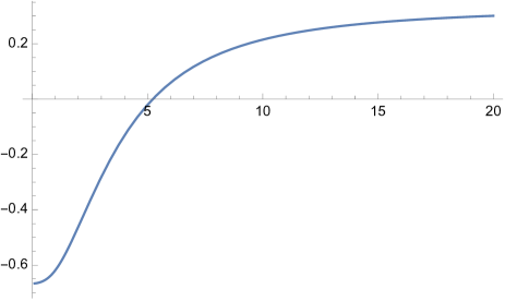
Figure 2: The dependence $\omega(H)$ at fixed value of the mass $m=2$.

Apparently, in the high temperature regime $H\gg m$ one finds the conformal value $\omega=1/3$, whereas in the opposite low temperature limit $H\ll m$ one gets $\omega=-2/3$. Note that this deviates from the result for a free gas in flat space, which has $\omega=0$ in the latter limit. In appendix C we will see the origin of the value $\omega=-2/3$ in the $m/H\to\infty$ limit.

However, like for a free gas in flat space with

$$\begin{split}\rho=\int{d^{3}k\over(2\pi)^{3}}{w\over e^{2\pi\omega/H}-1}=\int_{m}^{\infty}{d\omega\over 2\pi^{2}}\sqrt{\omega^{2}-m^{2}}{w^{2}\over e^{2\pi\omega/H}-1}\end{split}$$ (2.62)

where $w^{2}=\vec{k}^{2}+m^{2}$, for $H\ll m$ the energy density is exponentially suppressed. This can be seen in figures 3 and 4, where we plotted the energy density against the mass at fixed value of $H$ and against the temperature $H$ at fixed value of $m$.

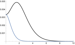
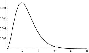
Figure 3: One the left: The dependence $\rho(m)$ at fixed value of the temperature $H=2$. The black curve is the expression (2.58), whereas the blue curve the flat space result (2.62). On the right: The difference of the two curves.

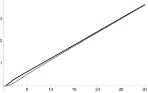
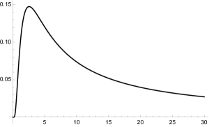
Figure 4: One the left: The dependence $\rho^{1\over 4}(H)$ at fixed value of the mass $m=2$. The black curve is the expression (2.58), whereas the blue curve the flat space result (2.62). On the right: The difference of the two curves.

Apparently, in the intermediate regime $m\sim H$ or equivalently $\lambda_{c}\sim\ell_{\rm dS}$, the two curves differ and show kind of a resonant behavior, while in the limiting low and high temperature regimes they essentially agree. Note that the main difference between the two expressions for $\rho$ is that, opposed to the free gas result (2.62), in (2.58) $\omega$ takes values in the full interval $0\leq\omega<\infty$.

In case we now have a tower of massive states with masses $m_{i}$, like in string theory, it is clear that the main contribution to the energy density (and also the pressure) at a fixed temperature $T=H/(2\pi)$ comes from those states with masses below $T$, i.e. $m_{i}\ll H$. As we have seen the contribution from states with masses $m_{i}\gg H$ is exponentially suppressed. Moreover, the scaling of $\rho$ with $H$ can already be determined from the flat space thermal expression for the energy density (2.62). Recall from the previous section that it is this scaling that determines the scaling of the quantum break time.

Even though we do not know how all the steps of this computation can be generalized to string theory, the simple form of the flat space contribution allows for a well- motivated guess.

Assumption 3: Also in string theory on dS space there will be a flat space thermal contribution to the energy density and pressure that can be evaluated from the well known stringy expressions for the perturbative thermal one-loop partition function and the resulting free energy.

We will make this more concrete in the following section.

3 Thermodynamics of string theory

Motivated by the discussion in the previous section, we now consider the thermodynamics of strings at finite temperature in flat space. Here the story is a bit more intricate than in field theories, mainly due to the existence of thermal winding modes and the consistency condition of modular invariance of the thermal partition function.

3.1 Free energy of strings at finite temperature

To make this paper self-contained, let us recall in this section some salient features of the description of strings at finite temperature (see e.g. [90, 91, 59, 92]), where the main focus is on the string theory generalization of the free energy and the energy density.

First, let us consider a boson of mass $m$ at fixed temperature $T$ in an $n$-dimensional space-time. In this case, the free energy density ${\cal F}=F/V$ is defined in the usual way as

$$\begin{split}{\cal F}_{b}(T)=-T\log Z_{b}(T)\,,\qquad{\rm where}\quad Z_{b}(T)=\prod_{p}{1\over 1-e^{-{E\over T}}}\end{split}$$ (3.1)

with the dispersion relation $E^{2}=p^{2}+m^{2}$. Employing the relation

$$\begin{split}\log(1-e^{-{E\over T}})={1\over 2}\sum_{m\in\mathbb{Z}}\log(E^{2}+4\pi^{2}m^{2}T^{2})\,,\end{split}$$ (3.2)

one can express the free energy as

$$\begin{split}{\cal F}_{b}(T)={T\over 2}\int{d^{n-1}p\over(2\pi)^{n-1}}\sum_{m\in\mathbb{Z}}\log\big{(}E^{2}+4\pi^{2}m^{2}T^{2}\big{)}\,,\end{split}$$ (3.3)

involving the infinite sum over the so-called Matsubara modes $m$. For a fermion, the analogous expression involves a sum over half-integer Matsubara modes

$$\begin{split}{\cal F}_{f}(T)=-{T\over 2}\int{d^{n-1}p\over(2\pi)^{n-1}}\sum_{m\in\mathbb{Z}}\log\big{(}E^{2}+4\pi^{2}\big{(}m+{\textstyle{1\over 2}}\big{)}^{2}T^{2}\big{)}\,.\end{split}$$ (3.4)

Identifying $R=1/(2\pi T)$, one can interpret the Matsubara modes as Kaluza-Klein modes of a circle compactification, whose contribution to the energy is as usual $E^{2}_{\rm KK}=m^{2}/R^{2}$. Therefore, the free energy of a gas of particles at temperature $T$ in $d=n-1$ (spatial) dimensions takes the same form as the $n$-dimensional vacuum energy compactified on a Wick-rotated time direction with radius $R=1/(2\pi T)$.

This picture can be generalized to string theory fairly straightforwardly. Employing the usual steps for computing string partition functions, one arrives at the following general expression for the free energy of a string at temperature $T$ moving in $n$ uncompactified (flat) dimensions (in string frame)

$$\begin{split}{\cal F}(T)=-{T\over 2}\left({M_{s}\over 2\pi}\right)^{n-1}\int_{\cal F}{d^{2}\tau\over\tau_{2}^{2}}{1\over\tau_{2}^{{n\over 2}-1}}Z_{\rm string}(\tau,\overline{\tau};T)\,,\end{split}$$ (3.5)

where the integral over the continuous momenta $p_{i}$, $i=1,\ldots,n-1$ has already been performed and we absorbed a factor of $\sqrt{\tau_{2}}$ into $Z_{\rm string}$ (see eq.(3.6) below). Hence, the string partition function $Z_{\rm string}$ is over the remaining string modes, i.e. the string oscillator modes, internal KK and winding modes and the Matsubara modes for the thermal circle compactification. Concerning the latter, one has to be a bit more careful, as in string theory a circle compactification not only leads to KK modes but also to winding modes. Moreover, one has to make sure that (space-time) bosons couple to integer and fermions to half-integer Matsubara modes in such a way that the final expression still features modular invariance.

The resolution to all these issues can be best described in terms of a string orbifold construction. The thermal partition function is closely related to a winding Scherk-Schwarz orbifold (WSS), i.e. a string theory compactification on $S^{1}/(-1)^{F}S_{w}$ with radius $R=1/(2\pi T)$. Here $F$ denotes the space-time fermion number and $S_{w}$ the winding shift that acts as $S_{w}:|m,n\rangle\to(-1)^{n}|m,n\rangle$ on a KK/winding mode. To describe the general form of the orbifold partition function let us introduce the following lattice contribution

$$\begin{split}Z_{\rm circ}(m,n)=\sqrt{\tau_{2}}\sum_{m,n}q^{{\alpha^{\prime}\over 4}({m\over R}+{nR\over\alpha^{\prime}})^{2}}\;\overline{q}^{{\alpha^{\prime}\over 4}({m\over R}-{nR\over\alpha^{\prime}})^{2}}\,,\end{split}$$ (3.6)

where $(m,n)$ indicate over which range the KK/winding modes run. Denoting

$$\begin{split}{\cal E}_{0}&=Z_{\rm circ}(m,2n)\,,\qquad\qquad{\cal E}_{1/2}=Z_{\rm circ}(m+{\textstyle{1\over 2}},2n)\,,\\ {\cal O}_{0}&=Z_{\rm circ}(m,2n+1)\,,\qquad{\cal O}_{1/2}=Z_{\rm circ}(m+{\textstyle{1\over 2}},2n+1)\,,\end{split}$$ (3.7)

the orbifold partition function in the untwisted sector can be generally expressed as

$$\begin{split}Z^{\rm(WSS)}_{\rm u}(R)=Z_{B}\,{\cal E}_{0}(R)-Z_{F}\,{\cal O}_{0}(R)\,,\end{split}$$ (3.8)

where $Z_{B/F}$ are the space-time boson/fermion contributions of the theory before the orbifold. Applying modular $T$ and $S$ transformations a twisted sector will appear which can generally be expressed as

$$\begin{split}Z^{\rm(WSS)}_{\rm t}(R)=Z^{(1)}_{t}\,{\cal E}_{1/2}(R)+Z_{t}^{(2)}\,{\cal O}_{1/2}(R)\,,\end{split}$$ (3.9)

where the form of $Z^{(1,2)}_{t}$ depends on the theory in question. The sum of the untwisted and the twisted partition functions define the modular invariant partition function $Z^{\rm(WSS)}$ of the WSS orbifold, where the temperature dependence solely resides in the lattice sums (3.7).

This is not yet the thermal partition function, but is closely related. For the final step, let us consider the behavior of (3.7) under modular transformations. Under a modular T-transformation ${\cal E}_{0},{\cal E}_{1/2},{\cal O}_{0}$ are invariant whereas ${\cal O}_{1/2}$ receives a minus sign. The action of a modular S-transformation is given by

$$\begin{split}S={1\over 2}\left(\begin{matrix}1&1&1&1\\ 1&1&-1&-1\\ 1&-1&1&-1\\ 1&-1&-1&1\end{matrix}\right)\,.\end{split}$$ (3.10)

Therefore, the “thermal map”

$$\begin{split}{\cal T}:\begin{cases}{\cal E}_{0}&\longleftrightarrow{\cal E}_{0}\\ {\cal E}_{1/2}&\longleftrightarrow{\cal O}_{0}\\ {\cal O}_{1/2}&\longleftrightarrow{\cal O}_{1/2}\end{cases}\end{split}$$ (3.11)

is an isomorphism and maps a modular invariant partition function to another modular invariant partition function. Applying this thermal map to the WSS orbifold, one gets the thermal partition function

$$\begin{split}Z^{\rm(T)}(T)=Z_{B}\,{\cal E}_{0}(T)-Z_{F}\,{\cal E}_{1/2}(T)+Z^{(1)}_{t}\,{\cal O}_{0}(T)+Z_{t}^{(2)}\,{\cal O}_{1/2}(T)\,.\end{split}$$ (3.12)

Note that now the untwisted space-time fermions indeed couple to half-integer KK Matsubara modes and we have used $R=1/(2\pi T)$.

3.2 Examples: type IIB and heterotic

Let us consider two simple ten-dimensional examples. First, recall that the type IIB partition function can be expressed as

$$\begin{split}Z_{\rm IIB}={1\over\eta^{8}(\tau)\eta^{8}(\overline{\tau})}\Big{(}\chi_{V}^{SO(8)}(\tau)-\chi_{S}^{SO(8)}(\tau)\Big{)}\Big{(}\overline{\chi}_{V}^{SO(8)}(\overline{\tau})-\overline{\chi}_{S}^{SO(8)}(\overline{\tau})\Big{)}\,,\end{split}$$ (3.13)

where the notation of the characters of the $\widehat{SO}(8)_{1}$ representations is standard. Compactifying the 10D type IIB theory on a circle and performing the winding Scherk-Schwarz orbifold leads to the partition function

$$\begin{split}Z_{\rm IIB}^{\rm(WSS)}(R)={1\over|\eta|^{16}}\Big{(}&(\chi_{V}\overline{\chi}_{V}+\chi_{S}\overline{\chi}_{S}){\cal E}_{0}-(\chi_{V}\overline{\chi}_{S}+\chi_{S}\overline{\chi}_{V}){\cal O}_{0}\\ +&(\chi_{O}\overline{\chi}_{O}+\chi_{C}\overline{\chi}_{C}){\cal E}_{1/2}-(\chi_{O}\overline{\chi}_{C}+\chi_{C}\overline{\chi}_{O}){\cal O}_{1/2}\Big{)}\,.\end{split}$$ (3.14)

This partition function interpolates between the type IIB superstring ($R\to 0$) and the non-supersymmetric tachyonic type 0B superstring ($R\to\infty$). Applying the thermal map (3.11) leads to the thermal partition function

$$\begin{split}Z_{\rm IIB}^{\rm(T)}(T)={1\over|\eta|^{16}}\Big{(}&(\chi_{V}\overline{\chi}_{V}+\chi_{S}\overline{\chi}_{S}){\cal E}_{0}-(\chi_{V}\overline{\chi}_{S}+\chi_{S}\overline{\chi}_{V}){\cal E}_{1/2}\\ +&(\chi_{O}\overline{\chi}_{O}+\chi_{C}\overline{\chi}_{C}){\cal O}_{0}-(\chi_{O}\overline{\chi}_{C}+\chi_{C}\overline{\chi}_{O}){\cal O}_{1/2}\Big{)}\,.\end{split}$$ (3.15)

One observes that the third term in (3.15) develops a tachyonic winding mode $(m,n)=(0,\pm 1)$ for temperatures larger than

$$\begin{split}T>{1\over\sqrt{2}}{M_{s}\over 2\pi}\,.\end{split}$$ (3.16)

This is nothing else than the Hagedorn temperature $T_{H}$, which generically is supposed to appear in theories with an exponential growth of degrees of freedom. However, the partition function reveals that it is an infrared effect associated with a massless (tachyonic) mode developing at $T_{H}$.

As a second example, we consider the ten-dimensional heterotic string with the partition function

$$\begin{split}Z={\Lambda^{G}(\overline{\tau})\over\eta^{8}(\tau)\eta^{8}(\overline{\tau})}\Big{(}\chi_{V}^{SO(8)}(\tau)-\chi_{S}^{SO(8)}(\tau)\Big{)}.\end{split}$$ (3.17)

Here the characters $\chi^{SO(8)}_{V}(\tau)$ and $\chi^{SO(8)}_{S}(\tau)$ arise from the left-moving fermions and $\Lambda^{G}(\overline{\tau})$ denotes the character of the $16$ right-moving bosons compactified on the root-lattice of $SO(32)$ or $E_{8}\times E_{8}$, respectively. Compactifying the 10D heterotic theory on a circle and performing the winding Scherk-Schwarz orbifold and applying the thermal map leads to the partition function

$$\begin{split}Z^{\rm(T)}(T)={\Lambda^{G}\over|\eta|^{16}}\Big{(}\chi_{V}^{SO(8)}{\cal E}_{0}-\chi_{S}^{SO(8)}{\cal E}_{1/2}-\chi_{C}^{SO(8)}{\cal O}_{0}+\chi_{O}^{SO(8)}{\cal O}_{1/2}\Big{)}\,.\end{split}$$ (3.18)

Note that in this case, on the level of characters one has $\chi_{S}^{SO(8)}=\chi_{C}^{SO(8)}$ and therefore $Z_{F}=Z_{t}^{(1)}$. Moreover, let us mention that the last term in (3.18) develops a tachyon in the window

$$\begin{split}(2-\sqrt{2}){M_{s}\over 2\pi}<T<(2+\sqrt{2}){M_{s}\over 2\pi}\,.\end{split}$$ (3.19)

Concretely, it is the KK/winding modes $\pm(-1/2,1)$ from ${\cal O}_{1/2}$ that can become tachyonic.

3.3 Tachyon condensation and a new phase of strings

We have seen in these two examples that at a certain critical temperature thermal tachyons appear in the spectrum. As argued in the seminal work by Atick-Witten [59], this rather indicates a phase transition (where the winding mode gets a non-zero vacuum expectation value) than a fundamental maximal temperature for strings. In fact, it is argued that this is a first order phase transition. Considering the effective theory of this condensing mode, they argue that also a tree-level (genus 0) contribution to the free energy is generated that strongly backreacts on the geometry. Therefore, analogous to the deconfining phase transition in QCD, this phase transition is expected to be dramatic and will reveal new degrees of freedom. As far as we are aware, there is no consensus yet what these new degrees of freedom of string theory at very high temperature (energy) are and by which theory they are described. It might be related to black-holes and/or a topological gravity theory.

Even though neither the meaning of the canonical ensemble nor the finiteness of the partition function is clear in this new phase, Atick-Witten argue that the extrapolation of the one-loop free energy (3.5) nevertheless gives a reasonable result for the high temperature dependence. For the type IIB superstring, this deviates from the usual field theory result and scales with $T$ like

$$\begin{split}{\cal F}(T)\sim\Lambda^{(1)}_{\rm 0B}\;T^{2}\,,\end{split}$$ (3.20)

where $\Lambda^{(1)}_{\rm 0B}$ denotes the (diverging) one-loop cosmological constant of the type 0B theory. For the heterotic string, it is the lower critical temperature $T_{H}=(2-\sqrt{2}){M_{s}\over 2\pi}$, at which a phase transition is expected to occur. However, at least formally the model is tachyon-free above a second critical temperature, which puts some more confidence on the scaling

$$\begin{split}{\cal F}(T)\sim\Lambda^{(1)}_{\rm het}\;T^{2}\end{split}$$ (3.21)

in the high temperature regime.

Let us mention that the quadratic temperature dependence could be explained by generalizing T-duality to the thermal circle (see also [94, 95]). Recall that a pure circle compactification of string theory enjoys T-duality acting as $R\to\alpha^{\prime}/R$, which will map for instance the two following Scherk-Schwarz orbifolds to one another [96]: type IIB on $S^{1}/(-1)^{F}S_{w}\longleftrightarrow$ type IIA on $S^{1}/(-1)^{F}S$, where $S$ denotes the left-right symmetric momentum shift. However, inspection reveals that there exists the slightly modified transformation $R\to\alpha^{\prime}/2R$, under which the lattice sums (3.7) transform as

$$\begin{split}\{{\cal E}_{0},{\cal E}_{1/2},{\cal O}_{0},{\cal O}_{1/2}\}\to\{{\cal E}_{0},{\cal O}_{0},{\cal E}_{1/2},{\cal O}_{1/2}\}\,,\end{split}$$ (3.22)

which is nothing else than the thermal map. Taking into account that this transformation acts on the temperature as

$$\begin{split}T\to{T_{c}^{2}/T}\,,\qquad{\rm with}\quad T_{c}=\sqrt{2}{M_{s}\over 2\pi}\,,\end{split}$$ (3.23)

we find the following transformation for the partition functions

$$\begin{split}Z^{\rm(T)}(T_{c}^{2}/T)=Z^{\rm(WSS)}(T)\,.\end{split}$$ (3.24)

This again shows the intricate relationship between these two partition functions. For the free energy this implies

$$\begin{split}{\cal F}^{\rm(T)}(T^{2}_{c}/T)=\left({T_{c}\over T}\right)^{2}{\cal F}^{\rm(WSS)}(T)\,.\end{split}$$ (3.25)

Applying this for instance to the type IIB example, one obtains

$$\begin{split}\lim_{T\to\infty}{\cal F}^{\rm(T)}(T)\sim T^{2}\lim_{R\to\infty}{\cal F}^{\rm(WSS)}(R)\sim T^{2}\Lambda^{(1)}_{\rm 0B}\,,\end{split}$$ (3.26)

which shows that the quadratic temperature dependence is a universal scaling relation. The energy density and the pressure are given in terms of the free energy density as

$$\begin{split}\rho={\cal F}-T{\partial{\cal F}\over\partial T}\,,\qquad p=-{\cal F}\,,\end{split}$$ (3.27)

from which one can derive

$$\begin{split}\rho^{\rm(T)}(T_{c}^{2}/T)=-\left({T_{c}\over T}\right)^{2}\rho^{\rm(WSS)}(T)\,.\end{split}$$ (3.28)

Note that both $T_{c}$ and $T_{H}$ are of the order of the string scale but differ by numerical prefactors.

To summarize: In the ultra high temperature region $T>T_{H}$ the condensed phase of strings is argued to have fewer degrees of freedom than naively expected and shows a quadratic scaling $\rho\sim T^{2}$ of the energy density with temperature. Support for this claim comes from a naive extrapolation of the perturbative expressions for the free energy into the regime $T>T_{H}$ and from a T-duality argument. Thus, quantum gravity at high energies behaves rather as a two-dimensional field theory. Intriguingly, the same observation was made in other approaches to quantum gravity, like the causal dynamical triangulation or asymptotic safety programs (see e.g.[55, 56]). In the following we will assume that this estimate is indeed correct and investigate what the consequences for quantum breaking and the swampland conjectures are. It is clearly very important to support the assumed scaling by, for instance, a direct computation for a candidate of a topological gravity theory or any other theory suggested to be valid beyond the Hagedorn transition.

4 dS quantum breaking for strings

Assume one has constructed an $n$-dimensional tree-level string model that features moduli stabilization in a tachyon-free dS or at least quasi dS phase. As we have seen in section 2, from the semiclassical approach of quantizing a free boson in the static patch, one obtains a matter contribution to the energy density and pressure. It is thermal with the Gibbons-Hawking temperature $T=H/(2\pi)$. Including this contribution in the Einstein equation, i.e. taking the quantum backreaction of the scalar into account, one finds that dS can no longer be a solution. Interpreting this as the source of quantum breaking of de Sitter, we aim to directly generalize this to string theory.

As was shown in section 2.4, for massive scalars, such as the ones in stringy towers of states, there is significant coincidence between the flat space result and the actual values of $\rho,p$ in static dS. More importantly, the scaling of these quantities with the temperature, which dictates the quantum breaking time, can be read off the flat space energy density. Hence, for our desired generalization to string theory, it seems sufficient to invoke the usual methods for the computation of the thermal partition function, which in turn directly leads to the energy and pressure temperature dependence.

Of course, for a concrete flux compactification with moduli stabilization the full one-loop thermal partition function cannot be determined explicitly. The models are usually described only in an effective supergravity approach, where only the lightest states are kept. Fortunately, the low ($T<T_{H}$) and the (naively extrapolated) high ($T>T_{H}$) temperature behavior turn out to be quite universal and do not depend on the full string theory spectrum. Let us discuss this in more detail.

4.1 Low temperature regime

Consider first the low-temperature regime and assume that in this regime there are no tachyons in the spectrum. In this case, all the winding modes with $n\neq 0$ are very massive and give a highly suppressed contribution to the free energy (3.5). Therefore, only the KK modes in ${\cal E}_{0}$ and ${\cal E}_{1/2}$ need to be considered which couple to $Z_{B}$ and $Z_{F}$ in (3.12). First, one can show that in the $T\to 0$ limit, the free energy approaches the 1-loop vacuum energy

$$\begin{split}\lim_{T\to 0}{\cal F}(T)=\Lambda^{(1)}_{0}\,.\end{split}$$ (4.1)

For finite $T$ the general behavior of the free energy is already revealed by considering the lightest states of mass $M_{b}$ and $M_{f}$ in $Z_{B}$ and $Z_{F}$. Then, the main contribution to the free energy is expected to arise from the following terms

$$\begin{split}{\cal F}(T)\sim-{T\over 2}&\left({M_{s}\over 2\pi}\right)^{n-1}\!\!\int_{1}^{\infty}{d\tau_{2}\over\tau_{2}^{n+1\over 2}}\biggl{[}e^{-\pi\tau_{2}\big{(}{M_{b}\over M_{s}}\big{)}^{2}}\,\sum_{m=-\infty}^{\infty}\exp\left(-2\pi\tau_{2}m^{2}({\textstyle{T\over T_{c}}})^{2}\right)\\[2.84544pt] &\phantom{aaaaaaaa}-e^{-\pi\tau_{2}\big{(}{M_{f}\over M_{s}}\big{)}^{2}}\,\sum_{m=-\infty}^{\infty}\exp\left(-2\pi\tau_{2}(m+{\textstyle{1\over 2}})^{2}({\textstyle{T\over T_{c}}})^{2}\right)\biggr{]}\,\end{split}$$ (4.2)

where we have carried out the integration over $\tau_{1}$ that gives the level-matching constraint. Note that here we are using the “self-dual” temperature $T_{c}$, which differs from the Hagedorn temperature only by an order one numerical prefactor. Using (4.2) one can straightforwardly compute the energy density $\rho$ via (3.27) and evaluate it numerically.

In figure 5 we show the resulting behavior of $\rho$ in the low-temperature regime in four dimensions. The right-hand side reveals that the temperature dependence for $T^{2}>{\rm Str}(M^{2})$ is indeed quartic, as expected from the Stefan-Boltzmann law. Performing an analogous computation in arbitrary dimension $n$, one can confirm the scaling ${\cal F}\sim T^{n}$. For even lower temperatures one finds the usual exponential drop-off $\exp(-m/T)$ expected from field theory for $T<m$.

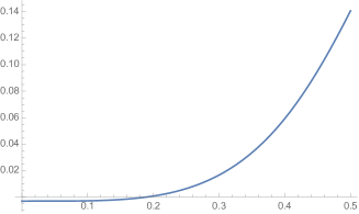
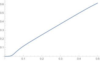
Figure 5: Left: The 1-loop energy density in the low temperature regime $T<T_{c}$ for $n=4$. Right: The fourth root of $\rho-\rho_{0}$. Choice of parameters: $m_{B}=0$, $m_{F}=0.2$.

Moreover, one can numerically check that the equation of state in the regime ${\rm Str}(M^{2})<T^{2}<T^{2}_{c}$ is indeed $p=\rho/(n-1)$.

To summarize, in the low temperature regime ${\rm Str}(M^{2})<T^{2}<T^{2}_{c}$ the string theoretic expression for the free energy nicely reproduces the expected low-energy field theory results and in particular the $\rho\sim T^{n}$ scaling.

4.2 High temperature regime

Increasing the temperature, we have already seen for the example of the type IIB superstring that one encounters a critical temperature $T_{H}$, where the appearance of thermal tachyons signals a phase transition of the system. It is clear that such tachyons can only arise from the terms ${\cal O}_{0}$ and ${\cal O}_{1/2}$, that are multiplied in (3.12) by the twisted sectors $Z_{t}^{(1,2)}$. Therefore, thermal tachyons can only appear when $Z_{t}^{(1,2)}$ themselves contain tachyons. The general expectation from the exponential growth of string states is that this is a generic phenomenon. However, the precise value of the temperature where this happens might be a model dependent question.

Following Atick-Witten [59], we now assume that the temperature dependence of the free energy in this new phase of string theory can still be reliably estimated from the expression (3.5), while ignoring the tachyonic divergences. In this high $T$ regime, the KK modes with $m\neq 0$ give a negligible contribution to the free energy so that solely the winding modes in ${\cal E}_{0}$ and ${\cal O}_{0}$ need to be considered. These couple to $Z_{B}$ and the twisted sector states $Z^{(1)}_{t}$ in (3.12). The lightest state in $Z_{B}$ will be a boson of mass $M_{b}$, while the lightest state in $Z^{(1)}_{t}$ could be a fermion or a boson of mass $M_{t}$. Thus, the main contribution to the free energy will come from the following terms

$$\begin{split}{\cal F}(T)\sim-{T\over 2}&\left({M_{s}\over 2\pi}\right)^{n-1}\!\!\int_{1}^{\infty}{d\tau_{2}\over\tau_{2}^{n+1\over 2}}\biggl{[}e^{-\pi\tau_{2}\big{(}{M_{b}\over M_{s}}\big{)}^{2}}\,\sum_{n=-\infty}^{\infty}\exp\left(-2\pi\tau_{2}n^{2}({\textstyle{T_{C}\over T}})^{2}\right)\\[2.84544pt] &\phantom{aaaaaaaa}\mp e^{-\pi\tau_{2}\big{(}{M_{t}\over M_{s}}\big{)}^{2}}\,\sum_{n=-\infty}^{\infty}\exp\left(-2\pi\tau_{2}(n+{\textstyle{1\over 2}})^{2}({\textstyle{T_{c}\over T}})^{2}\right)\biggr{]}\,.\end{split}$$ (4.3)

As shown in figure 6, independent of the number of dimensions one finds a quadratic behavior $\rho(T)\sim T^{2}$.

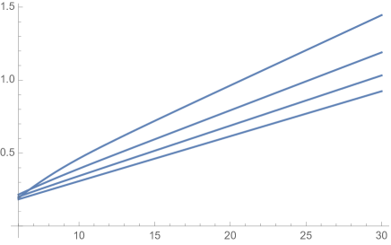
Figure 6: The square root of the energy density in the high temperature regime in dimensions $n=4,5,6,7$. Choice of parameters: $m_{B}=0.1$, $m_{F}=0.2$.

This can be easily proven from (4.3) by approximating the winding sum by a Gaussian integral. However, it also follows from the duality relation (3.28) if in the limit $R\to\infty$ the WSS one-loop partition function approaches $C^{(1)}$, i.e.

$$\begin{split}\rho(T)\to-\left({T\over T_{c}}\right)^{2}\lim_{R\to\infty}\rho^{\rm(WSS)}(R)=-C^{(1)}\left({T\over T_{c}}\right)^{2}\,.\end{split}$$ (4.4)

Furthermore, the equation of state in this regime is $p=\rho$. This suggests a drop in the number of degrees of freedom in this regime and rather shows the scaling behavior of a two-dimensional free gas. Let us summarize the main findings:

• In the low temperature regime, the string theoretic thermal energy density in $n$ dimensions behaves in the same way as in field theory, namely $\rho\sim T^{n}$ with equation of state $p={\rho\over n-1}$.

• In the high temperature regime, the scaling is universally $\rho\sim M^{n-2}_{s}\,T^{2}$ with $p=\rho$, independent of the number of dimensions.

Let us stress again, that this result was obtained by a naive extrapolation of the perturbative thermal string partition to a regime where it is not converging. The actual claim is that in the new phase beyond the Hagedorn transition, carrying out a bona fide computation will also lead to the same quadratic scaling behavior.

4.3 dS quantum breaking for strings

Now let us come back to our initial question about the behavior of the thermal quantum matter in a dS space. As mentioned, we are going to assume that the quantum backreaction approach again leads to a thermal quantum matter component, whose energy density and pressure are given in terms of the thermal string partition function (3.5) with $T=H/(2\pi)$. Of course this is a strong assumption, whose proof is beyond our computational abilities (at the moment), but it is a natural extrapolation of the quantum field theory results.

Up to this point, the computations in this section were done in the string frame. In string theory, the Planck scale is a derived quantity and related to the string scale via

$$\begin{split}M_{s}^{n-2}\sim{g_{s}^{2}M_{\rm pl}^{n-2}\over{\cal V}}\,,\end{split}$$ (4.5)

where ${\cal V}$ denotes the volume of the internal $10-n$ dimensional space in units of the string scale and $g_{s}$ the string coupling constant. Therefore, in the perturbative regime the string scale can be smaller than the Planck scale. Thus, in the following we consider this case with $g_{s}\ll 1$ and ${\cal V}\gg 1$.

The large volume implies that the free energy (4.3) will also contain a sum over light Kaluza-Klein modes. For a single circle direction and large radius $R$, this sum can be approximated by a Gaussian integral as

$$\begin{split}\sum_{m\in\mathbb{Z}}e^{-\pi\tau_{2}{m^{2}\over(M_{s}R)^{2}}}\approx M_{s}R\int_{-\infty}^{\infty}dx\,e^{-\pi\tau_{2}x^{2}}={M_{s}R\over\tau_{2}^{1/2}}\,.\end{split}$$ (4.6)

This shows the appearance of a multiplicative factor $M_{s}R\sim{\cal V}^{1/(10-n)}$ and the expected increase of the power of $\tau_{2}$ (see eq.(3.5)) in the decompactification limit.

Next we discuss the low and the high temperature phase separately, where following [57] we denote these two phases as phase II and phase I, respectively.

Low $T$ regime (phase II)

We have seen that for $T<T_{H}$ string theory nicely reproduces the field theory result for the energy density and the pressure. Thus, we expect to just recover the results from section 2.2, giving us the no eternal inflation constraints from the censorship of quantum breaking.

However, one needs to be a bit more careful. First, in section 2.2 it was implicitly assumed that the equations of motion are just the Friedmann equations resulting from the Einstein-Hilbert term. It is known that string theory generates higher derivative corrections to that. These $\alpha^{\prime}$ corrections involve higher curvature terms and for a dS background lead to $(H/M_{s})^{n}$ corrections to the left-hand side of the usual Friedmann equations. Therefore, at least at low temperatures, i.e. $H<M_{s}$, we are in the controlled regime.

Second, for ${\cal V}\gg 1$ but still working in an effective $n$-dimensional theory, the just observed appearance of the factor ${\cal V}$ in the free energy gives rise to a slight modification. Hence, in this case one gets $\rho\sim{\cal V}H^{n}$ such that the quantum breaking time (2.24) gets modified as

$$\begin{split}t_{Q}\sim{M_{\rm pl}^{n-2}\over{\cal V}H^{n-1}}\sim{M_{s}^{n-2}\over g_{s}^{2}H^{n-1}}\,.\end{split}$$ (4.7)

Censoring quantum breaking then leads to

$$\begin{split}{|V^{\prime}|\over V}\gtrsim g_{s}\left({H\over M_{s}}\right)^{n-2\over 2}\,,\end{split}$$ (4.8)

where we have set $M_{\rm pl}=1$. Note that the right-hand side still scales like $V^{n-2\over 4}$, as it appears in the no eternal inflation bound, but in practice imposes a stronger bound than (1.5). This implies that eternal inflation is censored by a string theoretic quantum breaking bound.

The appearance of the string scale instead of the Planck scale in $t_{Q}$ can be understood from the fact that for a large number of light species $N_{\rm sp}$ the effective cut-off of quantum gravity is not the Planck scale but the species scale [97]

$$\begin{split}\Lambda_{\rm sp}={M_{\rm pl}\over{N_{\rm sp}}^{\frac{1}{n-2}}}\,.\end{split}$$ (4.9)

To see what this means in our case, say one has an effective theory in $n$ dimensions that has a tower of states with masses $m_{N}=N\Delta m$, with a degeneracy of states at each mass level that scales like $N^{K}$. As in [98, 99, 100], the number of species lighter than the species scale is given by

$$\begin{split}N_{\rm sp}=\sum_{N=1}^{\Lambda_{\rm sp}/\Delta m}N^{K}\approx\left({\Lambda_{\rm sp}\over\Delta m}\right)^{K+1}\,.\end{split}$$ (4.10)

Consider compactifications on, for instance, isotropic $10-n$ dimensional tori or spheres. In this case one can simply deduce the degeneracy of KK modes as $K=9-n$ with a mass splitting $\Delta m=M_{s}/r$. Here $r$ denotes the radius in units of the string length. Using as well the relation (4.5) with ${\cal V}=r^{10-n}$, one can solve the above the relations for the species scale and get $\Lambda_{\rm sp}\sim M_{s}$. Therefore, for ${\cal V}\gg 1$ a tower of KK modes will become light so that the effective cut-off of quantum gravity becomes the string scale instead of the Planck scale. This makes it less surprising that in the relations above the string scale appears and not the Planck scale, as in the simple $n$-dimensional field theory result where no large extra dimensions were included.

High $T$ regime (phase I)

Next we consider the high temperature regime $T>T_{H}$ with its proposed universal 2D-like scaling behavior. This means that we study a dS space with $H>M_{s}$, a regime that is usually not considered in any string theory realization. In fact, one normally employs an effective field theory description of string cosmology that is beyond control in this regime, where $\alpha^{\prime}$ corrections will be substantial.

Indeed, the just discussed $H/M_{s}$ corrections to the left-hand side of the Friedmann equations are now non-negligible and it is a priori not clear how to extrapolate the latter beyond the phase transition. Remarkably, after identifying the temperature with the curvature of de Sitter space, also from this perspective one is losing control at $H\sim M_{s}\sim T_{H}$.

On the contrary, the methods we used for the description of the thermal string theory partition function or its relative, the WSS compactification, are of CFT type and are capturing in principle all $\alpha^{\prime}$ corrections (with $g_{s}\ll 1$ still in the perturbative regime). In fact, the scaling $\rho\sim M^{n-2}_{s}\,T^{2}$ was very generic and not depending on the many details of the remaining part of the partition function, i.e. $Z_{B/F}$ and $Z^{(1,2)}_{t}$.

We now proceed under the working assumption that in phase I, even though it is largely unknown, the two following aspects hold:

• At leading order, the equation of motion is still given by Einstein’s equations, i.e. in this regime there exists a controlled gravity theory.

• The energy density scales quadratically with the temperature.

Taking also the extra factor of ${\cal V}\sim(M_{s}R)^{10-n}$ into account, in Einstein-frame the $n$-dimensional one-loop thermal energy density can be written as

$$\begin{split}\rho=\kappa_{n}\,g_{s}^{2}\,M^{n-2}_{\rm pl}H^{2}\,.\end{split}$$ (4.11)

Now proceeding as in section 2.2, for this new (stringy) quantum matter component with equation of state parameter $w_{m}=1$, one finds a decay of the dS vacuum with a life-time

$$\begin{split}t_{Q}\sim{1\over g_{s}^{2}\,H}\,.\end{split}$$ (4.12)

Note that this scales precisely as suggested in [32, 33], namely $t_{Q}\sim 1/(\alpha H)$ with $\alpha\sim g_{s}^{2}$. As mentioned in the introduction, $\alpha$ denotes the quantum interaction strength. Censoring quantum breaking and assuming that also in phase I there can be a scalar field with a scalar potential, one now gets for the slow-roll parameter a lower bound

$$\begin{split}{|V^{\prime}|\over V}\gtrsim c\,g_{s}\,.\end{split}$$ (4.13)

Note that the right-hand side is independent of the potential $V$ in any space-time dimension, but still scales like $g_{s}$ and hence is not a pure $c$-number as in the dS conjecture and the asymptotic limit of TCC.

However, it might be that this perturbative factor of $g_{s}$ is just an artefact of the extrapolation of the one-loop thermal partition function to the high temperature phase that appears after tachyon condensation. Recalling from section 3.3 that tachyon condensation induces a tree-level contribution to the free energy, one could very well imagine that by directly performing the computation in this mysterious phase of string theory, the factor of $g_{s}^{2}$ in (4.11) will turn out to be absent such that $\alpha=\mathcal{O}(1)$.

Concluding remarks

Let us schematically summarize the main results about quantum breaking in string theory. In figure 7 we display the left-hand side of the Friedmann equations and the scaling of the energy density $\rho$ in the low and high temperature phases of string theory.

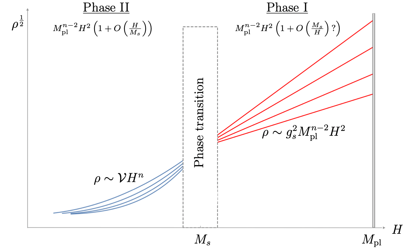
Figure 7: Schematic behavior of the square root of the energy density in the perturbative case with $M_{s}\ll M_{\rm pl}$ for dimensions $n=4,5,6,7$.

The energy density changes from $n$-dependent at low temperatures (phase II) to the universal $\sim H^{2}$ behavior at high temperatures (phase I). Moreover, in phase II the left-hand side of the Friedmann equations is under control and at leading order just given by the term following from Einstein’s equations, whereas in phase I we were just assuming that a similar story holds. Recall that in phase II we could employ computational methods from perturbative string theory to really derive the quantities in question, whereas for the high energy phase I we had to rely on reasonable assumptions that still need to be confirmed by a bona fide computation in e.g. a topological gravity theory.

The induced quantum break time $t_{Q}$ and the corresponding bound on $|V^{\prime}|/V$, denoted as $B(H)$, are shown in figure 8. It is clear that the universal quadratic scaling leads to a stronger bound for $|V^{\prime}|/V$. Note that in these simplified figures we are ignoring the $n$-dependent constant prefactors.

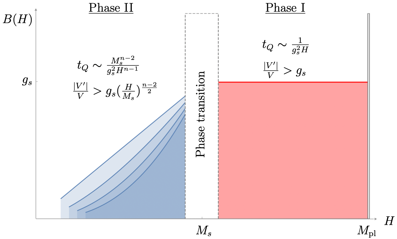
Figure 8: Schematic behavior of lower bound $B(H)$ in the perturbative case with $M_{s}\ll M_{\rm pl}$ for dimensions $n=4,5,6,7$. Shading corresponds to quantum breaking excluded region for $|V^{\prime}|/V$.

Let us end this section with a couple of remarks. We indeed found the same bounds as have been derived from the TCC, though now in different energy regimes. In phase II we find the weaker no eternal inflation bound, that is now the bound in all quasi dS models resulting from string theory in phase II, i.e. with $H<M_{s}$. Note that this seems to be consistent with TCC, where the stronger dS swampland bound only applies asymptotically, whereas as demonstrated in [25] one can find effective potentials satisfying TCC but just marginally excluding eternal inflation.

In the quantum break time approach, the strong bound from the dS swampland conjecture is the bound in phase I, a regime that has not yet been investigated for dS vacua in string theory/quantum gravity. We note that the asymptotic field limit in phase II is sort of at the boundary. In fact, according to the Emergent String Conjecture [101], an infinite distance limit in any quantum gravity theory is either an effective decompactification limit or a limit in which a critical string becomes weakly coupled and tensionless compared to the Planck scale. In the latter case, it also has to be included in the thermal partition function. Therefore, both in the decompactification limit and for the tensionless string case, in the limit $\phi\to\infty$ the string scale $M_{s}$ goes to zero and phase II disappears. This might be an explanation why for asymptotic field values one already encounters the stronger bound residing actually in phase I.

If indeed in the low $H$ phase only the weaker constraint $|V^{\prime}|/V\gtrsim c\,V^{n-2\over 4}$ was imposed by quantum gravity, it would leave much more room for string theory realizations of inflation and quintessence. For instance, in four space-time dimensions it leads to the maximal number of e-foldings ${\cal N}_{\rm max}\sim M_{s}^{2}/H^{2}$. On the other side, the stronger constraint in phase I would forbid a sufficiently long period of inflation in this high temperature phase of the universe leaving room for the alternative scenario of Agrawal, Gukov, Obied, Vafa [57], utilizing precisely the presumed topological gravity theory valid in this regime. Of course, all this is still very speculative and more research is needed.

As observed recently in [54], up to logarithmic corrections, the stronger bound in phase I implies that the life-time $t_{\rm dec}$ of dS is shorter than the scrambling/thermalization time $t_{s}\sim t_{Q}$. Thus, one might suspect that our argument breaks down, as we were initially assuming that the system is in the thermal Bunch-Davies vacuum. However, logically our arguments and conclusions are consistent with [54]. The logical chain can be summarized as

$$\begin{split}&{\rm dS\ is\ thermal\ }{\rm with}\ t_{\rm dec}>t_{s}\Longrightarrow{\rm QB\ takes\ place+censorship}\Rightarrow\\[5.69046pt] &\Rightarrow t_{\rm dec}<t_{Q}\Longrightarrow{\rm not\ thermal\ as\ }t_{\rm dec}<t_{s}\,,\end{split}$$ (4.14)

which is a contradiction to the initial assumption. Therefore, this assumption is not correct and the system decays before thermalization. But that is exactly what we intended to show, so our analysis can also be seen as a consistency check.

5 Conclusions

In this paper we have developed a line of arguments that mutually support the various assumptions made. We are not claiming that all steps are bulletproof and beyond doubt, but we think that we have at least uncovered potentially intricate relationships among some of the very basic issues in string theory/quantum gravity both from a bottom-up semiclassical approach and from a top-down string theoretic approach.

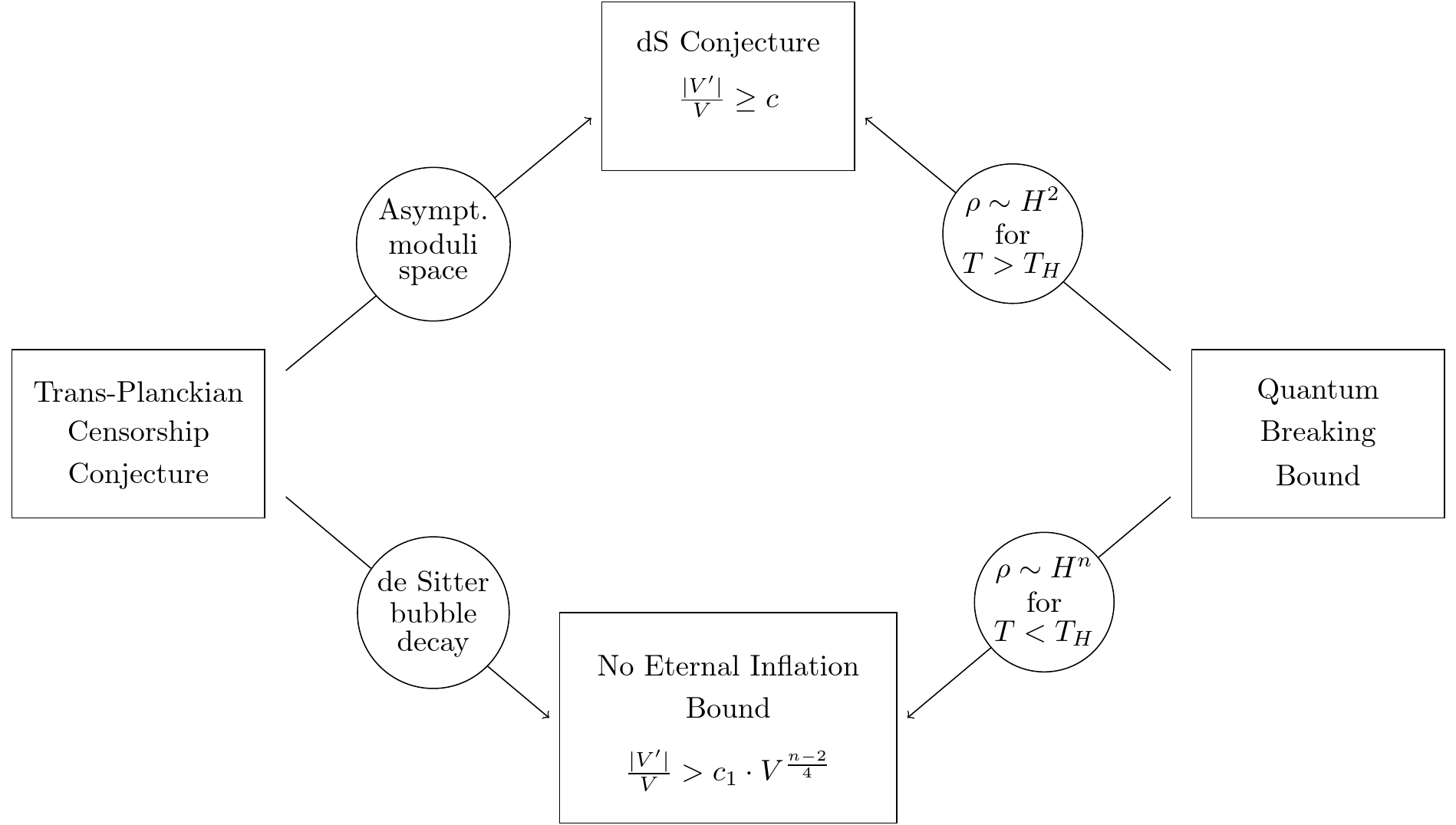
Figure 9: Schematic depiction of bounds for n-dimensional $V$ and their origin.

More concretely, as shown in the (now complete) figure 9, we have argued that the censorship of quantum breaking does imply both the no eternal inflation bound and the (refined) dS swampland conjecture in the low and high energy regimes, respectively, under the following assumptions:

• Quantum breaking can be determined by taking the backreaction of the semiclassical quantum energy-momentum tensor in the static patch into account.

• The essential scaling with the Gibbons-Hawking temperature can be deduced already from the analogous flat space energy-momentum tensor. The different IR behavior from modes with $\omega<m$ does only affect overall numerical prefactors.

• All these features extend to string theory on dS spaces in a straightforward manner.

• In the high temperature phase of string theory, independently of the number of space time dimensions, the energy density universally scales as $\rho\sim T^{2}$ and at leading order the equation of motion is still given by Einstein’s equations of gravity.

If true, the consequences of censoring quantum breaking are very similar to those that can be inferred from the trans-Planckian censorship conjecture, but now implying the no eternal inflation bound for low and the refined dS swampland conjecture for high Gibbons-Hawking temperatures. It would be worthwhile to find a more direct relation between the TCC and quantum breaking and understand the appearance of the $\log$-corrections also from the quantum breaking perspective. Moreover, it would be interesting to check whether the quantum breaking approach can also imply some of the other swampland conjectures that are interconnected with TCC, such as the swampland distance conjecture. Another intriguing question is whether the string theoretic high $T$ quantum break time could also be derived directly in the framework of decoherence presented in the work of Dvali-Gomez-Zell [30].

As a a further consequence of our assumptions we are led to the conjecture that eternal Minkowski space is not a solution of quantum gravity, either. This seems to be a bold conjecture that however has already some support from string theory constructions [84]. Of course, it would be interesting to study this further and in particular to see how for extended supersymmetry $N\geq 2$ this conclusion could be avoided.

Finally, maybe the most exciting aspect of our analysis is the appearance of the high energy regime of string theory. This also prominently appeared in the recent proposal [57] that the early history of the universe is not described by inflation but by a topological gravity theory. It would be intriguing to identify the nature of this topological theory and perform computations directly there, as for instance confirming the quadratic high temperature scaling of the free energy.

Acknowledgments

We would like to thank Irene Valenzuela for helpful correspondence and Rafa Álvarez-García, Max Brinkmann, Marco Scalisi and Lorenz Schlechter for useful discussions and comments on the draft. We also thank Lars Aalsma, Tommi Markkanen, Gary Shiu and Jan Pieter van der Schaar for enlightening critical discussions on a first version of this paper.

Appendix A Computation of normalization constants

In section 2.3 we mentioned that by imposing the commutation relations we can determine the normalization constants as (2.43). Here we perform the corresponding calculations. We start by writing down the commutation relations of $\Phi(r,\theta,\tau)$

$$\begin{split}[\Phi(r,\theta,\tau),&\dot{\Phi}(r^{\prime},\theta^{\prime},\tau)]=-\frac{i}{g^{\tau\tau}\sqrt{-g}}\,\delta(r-r^{\prime})\,\delta(\theta-\theta^{\prime})\,,\\ \end{split}$$ (A.1)

$$\begin{split}[\Phi(r,\theta,\tau),&\Phi(r^{\prime},\theta^{\prime},\tau)]=[\dot{\Phi}(r,\theta,\tau),\dot{\Phi}(r^{\prime},\theta^{\prime},\tau)]=0\,.\end{split}$$ (A.2)

Furthermore, by requiring the usual commutation relations for the creation and annihilation operators

$$\begin{split}[\hat{a}_{L\lambda\omega},\hat{a}^{\dagger}_{L^{\prime}\lambda^{\prime}\omega^{\prime}}]=\delta(\omega-\omega^{\prime})\,\delta_{LL^{\prime}}\,\delta_{\lambda\lambda^{\prime}}\,,\\ [\hat{a}_{L\lambda\omega},\hat{a}_{L^{\prime}\lambda^{\prime}\omega^{\prime}}]=[\hat{a}^{\dagger}_{L\lambda\omega},\hat{a}^{\dagger}_{L^{\prime}\lambda^{\prime}\omega^{\prime}}]=0\end{split}$$ (A.3)

we get

$$\begin{split}-i\int d\Omega\int_{0}^{\frac{1}{H}}dr\,\frac{r^{n-2}}{1-H^{2}r^{2}}\,\Phi_{1}\overleftrightarrow{\nabla}_{\tau}\,\Phi_{2}^{*}\overset{!}{=}\delta(\omega-\omega^{\prime})\,\delta_{LL^{\prime}}\,\delta_{\lambda\lambda^{\prime}}\,.\end{split}$$ (A.4)

Due to the established orthogonality of the spherical harmonics this reduces to an equation purely for $f_{L\omega}(r)$

$$\begin{split}\int_{0}^{\frac{1}{H}}dr\,\frac{r^{n-2}}{1-H^{2}r^{2}}\,f_{L\omega}(r)\,f_{L\omega^{\prime}}^{*}(r)=\frac{1}{2\omega\,|N_{L\omega}|^{2}}\,\delta(\omega-\omega^{\prime})\,.\end{split}$$ (A.5)

To solve this integral we may utilize the equations of motion (LABEL:radialeom) to rewrite

$$\begin{split}&(\omega^{2}-\omega^{\prime}\,{}^{2})\int_{0}^{\frac{1}{H}(1-\frac{\epsilon}{2})}dr\,\frac{r^{n-2}}{1-H^{2}r^{2}}\,f_{L\omega}(r)\,f_{L\omega^{\prime}}^{*}(r)=\\ &r^{n-2}(1-H^{2}r^{2})\Big{(}f_{L\omega}(r)\frac{d}{dr}f_{L\omega^{\prime}}(r)-f_{L\omega^{\prime}}(r)\frac{d}{dr}f_{L\omega}(r)\Big{)}\bigg{|}_{r\rightarrow\frac{1}{H}(1-\frac{\epsilon}{2})}.\end{split}$$ (A.6)

Additionally, the hypergeometric function has nice transformation properties. With formula (15.3.6) of [103] we may recast $f_{L\omega}(r)$ given by (2.38) at $r\sim\frac{1}{H}$ as

$$\begin{split}f_{L\omega}(r)\sim&\frac{\Gamma(\textstyle L+\frac{n-1}{2})\,\Gamma(\textstyle-\frac{i\omega}{H})}{\Gamma(\textstyle\frac{1}{2}(L-\frac{i\omega}{H}+\mu_{+}))\,\Gamma(\textstyle\frac{1}{2}(L-\frac{i\omega}{H}+\mu_{-}))}\,(1-H^{2}r^{2})^{\frac{i\omega}{2H}}\,+\\ &\frac{\Gamma(\textstyle L+\frac{n-1}{2})\,\Gamma(\textstyle\frac{i\omega}{H})}{\Gamma(\textstyle\frac{1}{2}(L+\frac{i\omega}{H}+\mu_{+}))\,\Gamma(\textstyle\frac{1}{2}(L+\frac{i\omega}{H}+\mu_{-}))}\,(1-H^{2}r^{2})^{-\frac{i\omega}{2H}}\,.\end{split}$$ (A.7)

Using (LABEL:identityeom) and (A.7) we find (A.5) to be

$$\begin{split}&I_{\epsilon}=\int_{0}^{\frac{1}{H}(1-\frac{\epsilon}{2})}dr\,\frac{r^{n-2}}{1-H^{2}r^{2}}\,f_{L\omega}(r)\,f_{L\omega}^{*}(r)=\\ &\textstyle\frac{i}{H^{n-2}(\omega+\omega^{\prime})}\Big{[}n^{L}_{\omega^{\prime}\,}n^{L}_{\omega}\,e^{\frac{i}{2H}(\omega+\omega^{\prime})\ln(\epsilon)}-n^{L}_{-\omega^{\prime}}\,n^{L}_{-\omega}\,e^{-\frac{i}{2H}(\omega+\omega^{\prime})\ln(\epsilon)}\Big{]}+\\ &\textstyle\frac{i}{H^{n-2}(\omega^{\prime}-\omega)}\Big{[}n^{L}_{\omega^{\prime}}\,n^{L}_{-\omega}\,e^{\frac{i}{2H}(\omega^{\prime}-\omega)\ln(\epsilon)}-n^{L}_{-\omega^{\prime}}\,n^{L}_{\omega}\,e^{-\frac{i}{2H}(\omega-\omega^{\prime})\ln(\epsilon)}\Big{]},\,\end{split}$$ (A.8)

with

$$\begin{split}n^{L}_{\omega}=\frac{\Gamma(\textstyle L+\frac{n-1}{2})\,\Gamma(\textstyle\frac{i\omega}{H})}{\Gamma(\textstyle\frac{1}{2}(L+\frac{i\omega}{H}+\mu_{+}))\,\Gamma(\textstyle\frac{1}{2}(L+\frac{i\omega}{H}+\mu_{-}))}\,.\end{split}$$ (A.9)

By dropping the stronger oscillating terms we can write:

$$\begin{split}I_{\epsilon}=\frac{2\,|n^{L}_{\omega}|^{2}}{H^{n-2}\,(\omega^{\prime}-\omega)}\sin\Big{(}\textstyle\frac{(\omega^{\prime}-\omega)}{2H}\ln\big{(}\textstyle\frac{1}{\epsilon}\big{)}\Big{)}\xrightarrow{\epsilon\rightarrow 0}2\pi|n^{L}_{\omega}|^{2}\delta(\omega-\omega^{\prime}),\end{split}$$ (A.10)

where we used $\lim\limits_{\alpha\to 0}\frac{\sin(\alpha x)}{x}\rightarrow\pi\delta(x)$.
By comparing (A.5) and (A.10) we can finally read off the normalization $|N_{L\omega}|^{2}$ as

$$\begin{split}|N_{L\omega}|^{2}=\frac{H^{n-2}}{4\pi\omega}\,\frac{\big{|}\Gamma(\textstyle\frac{1}{2}(L+\frac{i\omega}{H}+\mu_{+}))\big{|}^{2}\;\big{|}\Gamma(\textstyle\frac{1}{2}(L+\frac{i\omega}{H}+\mu_{-}))\big{|}^{2}}{\big{|}\Gamma(\textstyle L+\frac{n-1}{2})\big{|}^{2}\;\big{|}\Gamma(\textstyle\frac{i\omega}{H})\big{|}^{2}}\,.\end{split}$$ (A.11)

Appendix B Computation of individual contributions to $T_{00}$ and $T_{rr}$

In this appendix we provide the general expressions for the constituents of the energy-momentum tensor components. We see that to first order in ${O}(Hr)$ $\langle g^{rr}m^{2}\Phi^{2}\rangle$ and $-\langle g^{00}m^{2}\Phi^{2}\rangle$ are identical:

$$\begin{split}\langle g^{rr}m^{2}\Phi^{2}\rangle&=m^{2}\langle\Phi^{2}\rangle+{O}(Hr)^{2}\,,\\ -\langle g^{00}m^{2}\Phi^{2}\rangle&=m^{2}\langle\Phi^{2}\rangle+{O}(Hr)^{2}\,.\\ \end{split}$$ (B.1)

$m^{2}\langle\Phi^{2}\rangle$ can be computed by using the $L=0$ mode expansion to first order in ${O}(Hr)$ (2.56):

$$\begin{split}m^{2}\langle\Phi^{2}\rangle&=m^{2}\Big{\langle}\Big{|}\int_{0}^{\infty}d\omega\,[\Phi_{0,\lambda=0,\omega}\hat{a}_{0,\lambda=0,\omega}+\text{H.C.}]\Big{|}^{2}\Big{\rangle}\\ &=m^{2}\int_{0}^{\infty}d\omega\,|\Phi_{0,\lambda=0,\omega}|^{2}\left[1+2\langle\hat{n}_{0,\lambda=0,\omega}\rangle\right]\\ &=m^{2}\int_{0}^{\infty}d\omega\,\frac{H^{n-3}\sinh\left[\textstyle\frac{\pi\omega}{H}\right]}{4\pi^{2}\Gamma(\frac{n-1}{2})^{2}}\,|\Gamma(\textstyle\frac{1}{2}(\frac{i\omega}{H}+\mu_{+}))|^{2}\,|\Gamma(\textstyle\frac{1}{2}(\frac{i\omega}{H}+\mu_{-}))|^{2}\\ &\hskip 163.60333pt\times|Y_{0,\lambda=0}|^{2}\left[1+\frac{2}{e^{2\pi\omega/H}-1}\right]\\ &=m^{2}\int_{0}^{\infty}d\omega\,\frac{H^{n-3}\sinh\left[\textstyle\frac{\pi\omega}{H}\right]}{4\pi^{\frac{n+3}{2}}\Gamma(\textstyle\frac{n-1}{2})}\,|\Gamma(\textstyle\frac{1}{2}(\frac{i\omega}{H}+\mu_{+}))|^{2}\,|\Gamma(\textstyle\frac{1}{2}(\frac{i\omega}{H}+\mu_{-}))|^{2}\\ &\hskip 260.34253pt\times\Theta\!\left({\textstyle\omega\over H}\right)\,.\end{split}$$ (B.2)

Similarly the other contributions to $T_{00}$ and $T_{rr}$ can be calculated, first off the temporal derivative term:

$$\begin{split}\langle g^{00}(\partial_{0}\Phi)^{2}\rangle&=-\langle(\partial_{0}\Phi)^{2}\rangle+{O}(Hr)^{2}\\ -\langle(\partial_{0}\Phi)^{2}\rangle&=-\Big{\langle}\Big{|}\int_{0}^{\infty}d\omega[-i\omega\Phi_{0,\lambda=0,\omega}\hat{a}_{0,\lambda=0,\omega}+\text{H.C.}]\Big{|}^{2}\Big{\rangle}\\ &=\int_{0}^{\infty}d\omega\,\omega^{2}\,|\Phi_{0,\lambda=0,\omega}|^{2}\,\left[1+2\langle\hat{n}_{0,\lambda=0,\omega}\rangle\right]\\ &=\int_{0}^{\infty}d\omega\,\frac{H^{n-3}\,\omega^{2}\sinh\left[\textstyle\frac{\pi\omega}{H}\right]}{4\pi^{\frac{n+3}{2}}\,\Gamma(\textstyle\frac{n-1}{2})}|\Gamma(\textstyle\frac{1}{2}(\frac{i\omega}{H}+\mu_{+}))|^{2}\,|\Gamma(\textstyle\frac{1}{2}(\frac{i\omega}{H}+\mu_{-}))|^{2}\\ &\hskip 256.0748pt\times\Theta\!\left({\textstyle\omega\over H}\right).\end{split}$$ (B.3)

The radial derivative term is then given by:

$$\begin{split}\langle g^{rr}(\partial_{r}\Phi)^{2}\rangle&=\langle(\partial_{r}\Phi)^{2}\rangle+{O}(Hr)^{2}\\ \langle(\partial_{r}\Phi)^{2}\rangle&=\Big{\langle}\Big{|}\partial_{r}\sum_{\lambda}\int_{0}^{\infty}d\omega\,[\Phi_{1,\lambda,\omega}\hat{a}_{1,\lambda,\omega}+\text{H.C.}]\Big{|}^{2}\Big{\rangle}\\ &=\int_{0}^{\infty}d\omega\,\frac{(n-1)H^{n-1}\,\Gamma(\textstyle\frac{n-1}{2})\sinh\left[\textstyle\frac{\pi\omega}{H}\right]}{4\pi^{\frac{n+3}{2}}\,\Gamma(\textstyle\frac{n+1}{2})^{2}}\,|\Gamma(\textstyle\frac{1}{2}(1+\frac{i\omega}{H}+\mu_{+}))|^{2}\\ &\hskip 156.49014pt\times|\Gamma(\textstyle\frac{1}{2}(1+\frac{i\omega}{H}+\mu_{-}))|^{2}\,\Theta\!\left({\textstyle\omega\over H}\right).\end{split}$$ (B.4)

All of the expressions above are evaluated to first order in ${O}(Hr)$, since we are interested in the energy density and pressure for an observer far away from the horizon.

Appendix C Limit $m\gg H$ in 4D

In this appendix we want to prove that the equation of state parameter for the 4D massive scalar field in the limit $m\gg H$ is $\omega=-2/3$. First we observe that in this regime we can approximate

$$\begin{split}\mu_{\pm}={3\over 2}\pm{1\over 2}\sqrt{1-4{m^{2}\over H^{2}}}\approx{3\over 2}\pm i{m\over H}\,.\end{split}$$ (C.1)

Next we employ the asymptotic formula for the gamma function [103]

$$\begin{split}\lim\limits_{|y|\to\infty}(2\pi)^{-\frac{1}{2}}\,\big{|}\Gamma(x+iy)\big{|}\,e^{\frac{1}{2}\pi|y|}\,|y|^{\frac{1}{2}-x}=1\,\end{split}$$ (C.2)

to derive for the combination of $\Gamma$-functions appearing in the general expressions (2.58) and (2.61) for $\rho$ and $p$

$$\begin{split}\big{|}\Gamma\big{(}{\textstyle{3\over 4}+{i\omega\over 2H}(\omega+m)}\big{)}\big{|}^{2}&\big{|}\Gamma\big{(}{\textstyle{3\over 4}+{i\omega\over 2H}(\omega-m)}\big{)}\big{|}^{2}\\[2.84544pt] &=\begin{cases}\frac{2\pi^{2}}{H}\,\sqrt{\omega^{2}-m^{2}}\,e^{-\frac{\pi\omega}{H}},&{\rm for\ }\omega>m\\[8.5359pt] \frac{2\pi^{2}}{H}\,\sqrt{m^{2}-\omega^{2}}\,e^{-\frac{\pi m}{H}},&{\rm for\ }\omega<m\end{cases}\end{split}$$ (C.3)

and

$$\begin{split}\big{|}\Gamma\big{(}{\textstyle{5\over 4}+{i\omega\over 2H}(\omega+m)}\big{)}\big{|}^{2}&\big{|}\Gamma\big{(}{\textstyle{5\over 4}+{i\omega\over 2H}(\omega-m)}\big{)}\big{|}^{2}\\[2.84544pt] &=\begin{cases}\frac{\pi^{2}}{2H^{3}}\,\sqrt{\omega^{2}-m^{2}}^{3}\,e^{-\frac{\pi\omega}{H}},&{\rm for\ }\omega>m\\[8.5359pt] \frac{\pi^{2}}{2H^{3}}\,\sqrt{m^{2}-\omega^{2}}^{3}\,e^{-\frac{\pi m}{H}},&{\rm for\ }\omega<m\,.\end{cases}\end{split}$$ (C.4)

Looking at the exponentials, it is clear that the main contribution comes from the integration region $\omega<m$, i.e. the one that is not present in the thermal flat space relation (2.62). Therefore, the main contributions to $\rho$ and $p$ can be simplified as

$$\begin{split}\rho\approx{1\over 3\pi^{2}}\int_{0}^{m}d\omega\,m^{2}\,\sqrt{m^{2}-\omega^{2}}\,e^{-\frac{\pi m}{H}}{\sinh({\pi\omega\over H})\over e^{2\pi\omega/H}-1}\end{split}$$ (C.5)

and

$$\begin{split}p\approx-{2\over 9\pi^{2}}\int_{0}^{m}d\omega\,m^{2}\,\sqrt{m^{2}-\omega^{2}}\,e^{-\frac{\pi m}{H}}{\sinh({\pi\omega\over H})\over e^{2\pi\omega/H}-1}\end{split}$$ (C.6)

which apparently satisfy $p=-{2\over 3}\rho$.

References

- [1] E. Mottola, “Particle Creation in de Sitter Space,” Phys. Rev. D 31 (1985) 754.
- [2] E. Mottola, “Thermodynamic instability of de Sitter space,” Phys. Rev. D 33 (1986) 1616–1621.
- [3] S. Kachru, R. Kallosh, A. D. Linde, and S. P. Trivedi, “De Sitter vacua in string theory,” Phys. Rev. D 68 (2003) 046005, hep-th/0301240.
- [4] C. Vafa, “The String landscape and the swampland,” hep-th/0509212.
- [5] E. Palti, “The Swampland: Introduction and Review,” Fortsch. Phys. 67 (2019), no. 6, 1900037, 1903.06239.
- [6] M. van Beest, J. Calderón-Infante, D. Mirfendereski, and I. Valenzuela, “Lectures on the Swampland Program in String Compactifications,” 2102.01111.
- [7] M. Graña and A. Herráez, “The Swampland Conjectures: A Bridge from Quantum Gravity to Particle Physics,” Universe 7 (2021), no. 8, 273, 2107.00087.
- [8] T. D. Brennan, F. Carta, and C. Vafa, “The String Landscape, the Swampland, and the Missing Corner,” PoS TASI2017 (2017) 015, 1711.00864.
- [9] U. H. Danielsson and T. Van Riet, “What if string theory has no de Sitter vacua?,” Int. J. Mod. Phys. D 27 (2018), no. 12, 1830007, 1804.01120.
- [10] G. Obied, H. Ooguri, L. Spodyneiko, and C. Vafa, “De Sitter Space and the Swampland,” 1806.08362.
- [11] P. Agrawal, G. Obied, P. J. Steinhardt, and C. Vafa, “On the Cosmological Implications of the String Swampland,” Phys. Lett. B 784 (2018) 271–276, 1806.09718.
- [12] M. P. Hertzberg, S. Kachru, W. Taylor, and M. Tegmark, “Inflationary Constraints on Type IIA String Theory,” JHEP 12 (2007) 095, 0711.2512.
- [13] F. Denef, A. Hebecker, and T. Wrase, “de Sitter swampland conjecture and the Higgs potential,” Phys. Rev. D 98 (2018), no. 8, 086004, 1807.06581.
- [14] D. Andriot, “On the de Sitter swampland criterion,” Phys. Lett. B 785 (2018) 570–573, 1806.10999.
- [15] H. Ooguri, E. Palti, G. Shiu, and C. Vafa, “Distance and de Sitter Conjectures on the Swampland,” Phys. Lett. B 788 (2019) 180–184, 1810.05506.
- [16] S. K. Garg and C. Krishnan, “Bounds on Slow Roll and the de Sitter Swampland,” JHEP 11 (2019) 075, 1807.05193.
- [17] A. Bedroya and C. Vafa, “Trans-Planckian Censorship and the Swampland,” JHEP 09 (2020) 123, 1909.11063.
- [18] G. Dvali, A. Kehagias, and A. Riotto, “Inflation and Decoupling,” 2005.05146.
- [19] C. P. Burgess, S. P. de Alwis, and F. Quevedo, “Cosmological Trans-Planckian Conjectures are not Effective,” JCAP 05 (2021) 037, 2011.03069.
- [20] T. Rudelius, “Conditions for (No) Eternal Inflation,” JCAP 08 (2019) 009, 1905.05198.
- [21] A. D. Linde, Particle physics and inflationary cosmology, vol. 5 of Contemp.Concepts Phys. 1990.
- [22] D. N. Page, “Space for both no boundary and tunneling quantum states of the universe,” Phys. Rev. D 56 (1997) 2065–2072, gr-qc/9704017.
- [23] P. Creminelli, S. Dubovsky, A. Nicolis, L. Senatore, and M. Zaldarriaga, “The Phase Transition to Slow-roll Eternal Inflation,” JHEP 09 (2008) 036, 0802.1067.
- [24] H. Matsui and F. Takahashi, “Eternal Inflation and Swampland Conjectures,” Phys. Rev. D 99 (2019), no. 2, 023533, 1807.11938.
- [25] A. Bedroya, M. Montero, C. Vafa, and I. Valenzuela, “de Sitter Bubbles and the Swampland,” Fortsch. Phys. 68 (2020), no. 11-12, 2000084, 2008.07555.
- [26] G. Barenboim, W.-I. Park, and W. H. Kinney, “Eternal Hilltop Inflation,” JCAP 05 (2016) 030, 1601.08140.
- [27] W. H. Kinney, “Eternal Inflation and the Refined Swampland Conjecture,” Phys. Rev. Lett. 122 (2019), no. 8, 081302, 1811.11698.
- [28] G. Dvali and C. Gomez, “Quantum Compositeness of Gravity: Black Holes, AdS and Inflation,” JCAP 01 (2014) 023, 1312.4795.
- [29] G. Dvali and C. Gomez, “Quantum Exclusion of Positive Cosmological Constant?,” Annalen Phys. 528 (2016) 68–73, 1412.8077.
- [30] G. Dvali, C. Gomez, and S. Zell, “Quantum Break-Time of de Sitter,” JCAP 06 (2017) 028, 1701.08776.
- [31] L. Aalsma, M. Parikh, and J. P. Van Der Schaar, “Back(reaction) to the Future in the Unruh-de Sitter State,” JHEP 11 (2019) 136, 1905.02714.
- [32] G. Dvali and C. Gomez, “On Exclusion of Positive Cosmological Constant,” Fortsch. Phys. 67 (2019), no. 1-2, 1800092, 1806.10877.
- [33] G. Dvali, C. Gomez, and S. Zell, “Quantum Breaking Bound on de Sitter and Swampland,” Fortsch. Phys. 67 (2019), no. 1-2, 1800094, 1810.11002.
- [34] S. Brahma, K. Dasgupta, and R. Tatar, “Four-dimensional de Sitter space is a Glauber-Sudarshan state in string theory,” JHEP 07 (2021) 114, 2007.00786.
- [35] S. Brahma, K. Dasgupta, and R. Tatar, “de Sitter Space as a Glauber-Sudarshan State,” JHEP 02 (2021) 104, 2007.11611.
- [36] H. Bernardo, S. Brahma, K. Dasgupta, and R. Tatar, “Crisis on Infinite Earths: Short-lived de Sitter Vacua in the String Theory Landscape,” JHEP 04 (2021) 037, 2009.04504.
- [37] P. C. W. Davies, S. A. Fulling, S. M. Christensen, and T. S. Bunch, “Energy Momentum Tensor of a Massless Scalar Quantum Field in a Robertson-Walker Universe,” Annals Phys. 109 (1977) 108–142.
- [38] T. S. Bunch and P. C. W. Davies, “Stress tensor and conformal anomalies for massless fields in a Robertson–Walker universe,” Proc. R. Soc. Lond.. 356 (1977) 569–574.
- [39] T. S. Bunch, “Calculation of the Renormalized Quantum Stress Tensor by Adiabatic Regularization in Two-Dimensional and Four-Dimensional Robertson-Walker Space-Times,” J. Phys. A 11 (1978) 603–607.
- [40] G. Gibbons and S. Hawking, “Cosmological Event Horizons, Thermodynamics, and Particle Creation,” Phys. Rev. D 15 (1977) 2738–2751.
- [41] T. Markkanen, “Decoherence Can Relax Cosmic Acceleration,” JCAP 11 (2016) 026, 1609.01738.
- [42] T. Markkanen, “Decoherence Can Relax Cosmic Acceleration: an Example,” JCAP 09 (2017) 022, 1610.06637.
- [43] T. Markkanen, “De Sitter Stability and Coarse Graining,” Eur. Phys. J. C 78 (2018), no. 2, 97, 1703.06898.
- [44] N. Arkani-Hamed, L. Motl, A. Nicolis, and C. Vafa, “The String landscape, black holes and gravity as the weakest force,” JHEP 06 (2007) 060, hep-th/0601001.
- [45] H. Ooguri and C. Vafa, “On the Geometry of the String Landscape and the Swampland,” Nucl. Phys. B 766 (2007) 21–33, hep-th/0605264.
- [46] H. Ooguri and C. Vafa, “Non-supersymmetric AdS and the Swampland,” Adv. Theor. Math. Phys. 21 (2017) 1787–1801, 1610.01533.
- [47] D. Kläwer, D. Lüst, and E. Palti, “A Spin-2 Conjecture on the Swampland,” Fortsch. Phys. 67 (2019), no. 1-2, 1800102, 1811.07908.
- [48] D. Lüst, E. Palti, and C. Vafa, “AdS and the Swampland,” Phys. Lett. B 797 (2019) 134867, 1906.05225.
- [49] M.-S. Seo, “Thermodynamic interpretation of the de Sitter swampland conjecture,” Phys. Lett. B 797 (2019) 134904, 1907.12142.
- [50] M.-S. Seo, “The entropic quasi-de Sitter instability time from the distance conjecture,” Phys. Lett. B 807 (2020) 135580, 1911.06441.
- [51] H. Geng, “Distance Conjecture and De-Sitter Quantum Gravity,” Phys. Lett. B 803 (2020) 135327, 1910.03594.
- [52] Q. Bonnefoy, L. Ciambelli, D. Lüst, and S. Lüst, “Infinite Black Hole Entropies at Infinite Distances and Tower of States,” Nucl. Phys. B 958 (2020) 115112, 1912.07453.
- [53] M. Lüben, D. Lüst, and A. R. Metidieri, “The Black Hole Entropy Distance Conjecture and Black Hole Evaporation,” Fortsch. Phys. 69 (2021), no. 3, 2000130, 2011.12331.
- [54] A. Bedroya, “de Sitter Complementarity, TCC, and the Swampland,” 2010.09760.
- [55] S. Carlip, “Spontaneous Dimensional Reduction in Short-Distance Quantum Gravity?,” AIP Conf. Proc. 1196 (2009), no. 1, 72, 0909.3329.
- [56] S. Carlip, “Dimension and Dimensional Reduction in Quantum Gravity,” Class. Quant. Grav. 34 (2017), no. 19, 193001, 1705.05417.
- [57] P. Agrawal, S. Gukov, G. Obied, and C. Vafa, “Topological Gravity as the Early Phase of Our Universe,” 2009.10077.
- [58] E. Witten, “Topological Gravity,” Phys. Lett. B 206 (1988) 601–606.
- [59] J. J. Atick and E. Witten, “The Hagedorn Transition and the Number of Degrees of Freedom of String Theory,” Nucl. Phys. B 310 (1988) 291–334.
- [60] D. J. Gross, “High-Energy Symmetries of String Theory,” Phys. Rev. Lett. 60 (1988) 1229.
- [61] B. Allen, “Vacuum States in de Sitter Space,” Phys. Rev. D 32 (1985) 3136.
- [62] N. A. Chernikov and E. A. Tagirov, “Quantum theory of scalar fields in de Sitter space-time,” Ann. Inst. H. Poincare Phys. Theor. A 9 (1968) 109.
- [63] T. Bunch and P. Davies, “Quantum Field Theory in de Sitter Space: Renormalization by Point Splitting,” Proc. Roy. Soc. Lond. A 360 (1978) 117–134.
- [64] N. Birrell and P. Davies, Quantum Fields in Curved Space. Cambridge Monographs on Mathematical Physics. Cambridge Univ. Press, Cambridge, UK, 2, 1984.
- [65] M. Spradlin, A. Strominger, and A. Volovich, “Les Houches lectures on de Sitter space,” in Les Houches Summer School: Session 76: Euro Summer School on Unity of Fundamental Physics: Gravity, Gauge Theory and Strings, pp. 423–453. 10, 2001. hep-th/0110007.
- [66] L. E. Parker and D. Toms, Quantum Field Theory in Curved Spacetime: Quantized Field and Gravity. Cambridge Monographs on Mathematical Physics. Cambridge University Press, 8, 2009.
- [67] L. Aalsma, A. Cole, E. Morvan, J. P. van der Schaar, and G. Shiu, “Shocks and Information Exchange in de Sitter Space,” 2105.12737.
- [68] L. Parker and S. Fulling, “Adiabatic regularization of the energy momentum tensor of a quantized field in homogeneous spaces,” Phys. Rev. D 9 (1974) 341–354.
- [69] T. Bunch, “Adiabatic regularization for scalar fields with arbitrary coupling to the scalar curvature,” J. Phys. A 13 (1980) 1297–1310.
- [70] N. Goheer, M. Kleban, and L. Susskind, “The Trouble with de Sitter space,” JHEP 07 (2003) 056, hep-th/0212209.
- [71] T. S. Bunch, “Stress Tensor of Massless Conformal Quantum Fields in Hyperbolic Universes,” Phys. Rev. D 18 (1978) 1844–1848.
- [72] B. DeWitt, “General Relativity: An Einstein Centenary Survey,” Univ. Pr., Cambridge, UK, 1979.
- [73] P. Candelas and J. S. Dowker, “Field theories on conformally related space-times: some global considerations,” Phys. Rev. D 19 (1979) 2902.
- [74] R. Bousso, A. Maloney, and A. Strominger, “Conformal vacua and entropy in de Sitter space,” Phys. Rev. D 65 (2002) 104039, hep-th/0112218.
- [75] P. Lagogiannis, A. Maloney, and Y. Wang, “Odd-dimensional de Sitter Space is Transparent,” 1106.2846.
- [76] P. Candelas and D. Deutsch, “On the vacuum stress induced by uniform acceleration or supporting the ether,” Proc. Roy. Soc. Lond. A 354 (1977) 79–99.
- [77] I. Antoniadis, P. O. Mazur, and E. Mottola, “Cosmological dark energy: Prospects for a dynamical theory,” New J. Phys. 9 (2007) 11, gr-qc/0612068.
- [78] P. R. Anderson and E. Mottola, “Quantum vacuum instability of “eternal” de Sitter space,” Phys. Rev. D 89 (2014) 104039, 1310.1963.
- [79] H. Matsui, “Instability of De Sitter Spacetime induced by Quantum Conformal Anomaly,” JCAP 01 (2019) 003, 1806.10339.
- [80] H. Matsui and N. Watamura, “Quantum Spacetime Instability and Breakdown of Semiclassical Gravity,” Phys. Rev. D 101 (2020), no. 2, 025014, 1910.02186.
- [81] P. M. Chesler and A. Loeb, “Holographic duality and mode stability of de Sitter space in semiclassical gravity,” JCAP 11 (2020) 010, 2003.05501.
- [82] R. Blumenhagen, M. Brinkmann, and A. Makridou, “Quantum Log-Corrections to Swampland Conjectures,” JHEP 02 (2020) 064, 1910.10185.
- [83] R. Blumenhagen, M. Brinkmann, D. Kläwer, A. Makridou, and L. Schlechter, “KKLT and the Swampland Conjectures,” PoS CORFU2019 (2020) 158, 2004.09285.
- [84] E. Palti, C. Vafa, and T. Weigand, “Supersymmetric Protection and the Swampland,” JHEP 06 (2020) 168, 2003.10452.
- [85] D. Polarski, “A Minimally Coupled Scalar Field on the Static De Sitter Space,” Phys. Rev. D 41 (1990) 442.
- [86] D. Polarski, “Massive scalar field on the static de Sitter space,” Phys. Rev. D 41 (1990) 2519–2524.
- [87] J. E. Avery and J. S. Avery, Hyperspherical Harmonics and Their Physical Applications. World Scientific, 2018.
- [88] E. Abdalla, K. Castello-Branco, and A. Lima-Santos, “Support of dS / CFT correspondence from space-time perturbations,” Phys. Rev. D 66 (2002) 104018, hep-th/0208065.
- [89] A. Higuchi, “Quantization of Scalar and Vector Fields Inside the Cosmological Event Horizon and Its Application to Hawking Effect,” Class. Quant. Grav. 4 (1987) 721.
- [90] R. Rohm, “Spontaneous Supersymmetry Breaking in Supersymmetric String Theories,” Nucl. Phys. B 237 (1984) 553–572.
- [91] E. Alvarez and M. Osorio, “Superstrings at Finite Temperature,” Phys. Rev. D 36 (1987) 1175.
- [92] K. R. Dienes, M. Lennek, and M. Sharma, “Strings at Finite Temperature: Wilson Lines, Free Energies, and the Thermal Landscape,” Phys. Rev. D 86 (2012) 066007, 1205.5752.
- [93] C. Angelantonj, C. Kounnas, H. Partouche, and N. Toumbas, “Resolution of Hagedorn singularity in superstrings with gravito-magnetic fluxes,” Nucl. Phys. B 809 (2009) 291–307, 0808.1357.
- [94] K. R. Dienes and M. Lennek, “Thermal duality confronts entropy: A New approach to string thermodynamics?,” hep-th/0312173.
- [95] K. R. Dienes and M. Lennek, “Adventures in thermal duality. 2. Towards a duality covariant string thermodynamics,” Phys. Rev. D 70 (2004) 126006, hep-th/0312217.
- [96] C. Angelantonj and A. Sagnotti, “Open strings,” Phys. Rept. 371 (2002) 1–150, hep-th/0204089. [Erratum: Phys.Rept. 376, 407 (2003)].
- [97] G. Dvali and M. Redi, “Black Hole Bound on the Number of Species and Quantum Gravity at LHC,” Phys. Rev. D 77 (2008) 045027, 0710.4344.
- [98] B. Heidenreich, M. Reece, and T. Rudelius, “The Weak Gravity Conjecture and Emergence from an Ultraviolet Cutoff,” Eur. Phys. J. C78 (2018), no. 4, 337, 1712.01868.
- [99] T. W. Grimm, E. Palti, and I. Valenzuela, “Infinite Distances in Field Space and Massless Towers of States,” JHEP 08 (2018) 143, 1802.08264.
- [100] B. Heidenreich, M. Reece, and T. Rudelius, “Emergence of Weak Coupling at Large Distance in Quantum Gravity,” Phys. Rev. Lett. 121 (2018), no. 5, 051601, 1802.08698.
- [101] S.-J. Lee, W. Lerche, and T. Weigand, “Emergent Strings from Infinite Distance Limits,” 1910.01135.
- [102] U. H. Danielsson and M. E. Olsson, “On thermalization in de Sitter space,” JHEP 03 (2004) 036, hep-th/0309163.
- [103] M. Abramowitz and I. A. Stegun, eds., Handbook of Mathematical Functions with Formulas, Graphs and Mathematical Tables. Dover Publications, Inc., New York, 1965.