Deterministic Certification to Adversarial Attacks via
Bernstein Polynomial Approximation

Abstract

Randomized smoothing has established state-of-the-art provable robustness against $\ell_{2}$ norm adversarial attacks with high probability. However, the introduced Gaussian data augmentation causes a severe decrease in natural accuracy. We come up with a question, “Is it possible to construct a smoothed classifier without randomization while maintaining natural accuracy?”. We find the answer is definitely yes. We study how to transform any classifier into a certified robust classifier based on a popular and elegant mathematical tool, Bernstein polynomial. Our method provides a deterministic algorithm for decision boundary smoothing. We also introduce a distinctive approach of norm-independent certified robustness via numerical solutions of nonlinear systems of equations. Theoretical analyses and experimental results indicate that our method is promising for classifier smoothing and robustness certification.

Introduction

Neural Network models achieve an enormous breakthrough in image classification these years but are vulnerable to imperceptible perturbations known as adversarial attacks, as evidenced by (Goodfellow, Shlens, and Szegedy 2015) (Szegedy et al. 2014). Since then, many researchers began to develop their adversarial attacks such as DeepFool (Moosavi-Dezfooli, Fawzi, and Frossard 2016), Jacobian based Saliency Map Attack (JSMA) (Papernot et al. 2016), CW attack (Carlini and Wagner 2017b), etc. On the other hand, researchers also attempted to build defense mechanisms that are invincible to adversarial attacks. Please see (Yuan et al. 2019) for the thorough surveys of adversarial attacks and defense approaches. However, we still have a long way to go in that making an indestructible machine learning model is still an open problem in the AI community.

Empirical defense strategies can be categorized into several groups. The first one is adversarial detection (Feinman et al. 2017) (Ma et al. 2018). However, (Carlini and Wagner 2017a) bypassed ten detection methods and showed that it is extremely challenging to detect adversarial attacks. The second one is denoising (Liao et al. 2018) (Xie et al. 2019) (Xu, Evans, and Qi 2018). The kind of methods is computationally inefficient (some works trained on hundreds of GPUs) but useful in practice. The third one is called adversarial training, which is the most effective but suffers from attack dependency (Tramèr et al. 2018) (Madry et al. 2018). In addition to the aforementioned methods, there are still various defense strategies proposed. (Athalye, Carlini, and Wagner 2018) showed that most of the defense methods are ineffective when encountering sophisticated designed attacks due to lack of a provable defense guarantee.

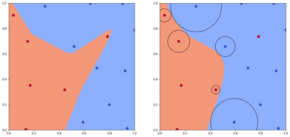
Figure 1: A 2D example to visualize our result. Left: The classifier’s decision boundary from the neural network is very “sharp”. Points near the sharp region are vulnerable to adversarial attacks. Right: We can see that the boundary of the classifier from our method is smoothed, and the certification (“safe zone”) is mostly accurate.

To avoid this arms race, a series of researches (Salman et al. 2019b) on provable defenses or certified robustness have emerged with theoretical guarantees. Specifically, for any point $x$, there is a set containing the provably robust $x$, implying that every point in this set gives the same prediction.

Assume that adversarial examples are caused due to the irregularity of the decision boundary. Randomized smoothing (Cohen, Rosenfeld, and Kolter 2019) introduced Gaussian random noise for smoothing the base classifier. Nonetheless, many challenges remain. Firstly, Gaussian data augmentation causes a severe decrease in natural accuracy. Secondly, the prediction and certification require numerous samples during inference, which is a time-consuming process. Thirdly, there is still a chance, even slightly, that the certification is inaccurate. In many applications, like self-driving vehicles, we do not want to take this kind of risk.

In this paper, we propose a new method to “smooth” the decision boundary of the classifier. Our method can also provide a “safe zone” that predicts the same class as the input deterministically. We use a 2D example to demonstrate our method in Figure 1. Note that the regions near the decision boundary are more comfortable to certify by our approach, while the areas far from the decision boundary are less accurate. It is due to the initial guess of the solver of nonlinear systems of equations. To overcome this problem, we set the error tolerance of the solution to an acceptable threshold (Virtanen et al. 2020). Furthermore, we care more about data near the decision boundary than those far away from it since we can find adversarial examples with our bare eyes if the attack is strong enough.

Our contributions are summarized as follows:

• To our knowledge, we are the first to introduce Bernstein polynomial into the adversarial example community for which we devise a deterministic algorithm to smooth the base classifier.

• Our method, compared with (Cohen, Rosenfeld, and Kolter 2019) and (Salman et al. 2019a), can maintain higher natural accuracy while achieving comparable robustness (certified accuracy) in CIFAR-10 (Krizhevsky, Hinton et al. 2009).

• We can certify a smoothed classifier with arbitrary norms (norm independent).

• Our method can be used in different aspects of machine learning beyond certified robustness, such as over-fitting alleviation.

Related Works

We roughly categorize adversarial defense researches into empirical defenses and certified defenses. Empirical defenses seem to be robust to existing adversarial perturbations but lack of formal robustness guarantee. In this section, we will study previous empirical defenses and certified defenses with the focus on randomized smoothing.

Empirical defenses

In practice, the best empirical defense is Adversarial Training (AT) (Goodfellow, Shlens, and Szegedy 2015) (Kurakin, Goodfellow, and Bengio 2017) (Madry et al. 2018). AT is operated by first generating the adversarial examples by projected gradient descent and then augmenting them into the training set. Although the classifier yielded based on AT is robust to most gradient-based attacks, it is still difficult to tell whether this classifier is undoubtedly robust. Moreover, adaptive attacks break most empirical defenses. A pioneering study (Athalye, Carlini, and Wagner 2018) showed that most of the methods are ineffective by using sophisticated designed attacks. To stop this arms race between attackers and defenders, some researchers try to focus on building a verification mechanism with a robustness guarantee.

Certified defenses

Certified defenses can be divided into exact (a.k.a “complete”) methods and conservative (a.k.a “incomplete”) methods. Exact methods are usually based on Satisfiability Modulo Theories solvers (Katz et al. 2017a) (Katz et al. 2017b) or mixed-integer linear programming (Tjeng, Xiao, and Tedrake 2019), but they are computationally inefficient. Conservative methods are guaranteed to find adversarial examples if they exist but might mistakenly judge a safe data point as an adversarial one (false positive) (Wong and Kolter 2018) (Wong et al. 2018) (Salman et al. 2019b) (Wang et al. 2018b) (Wang et al. 2018a) (Dvijotham et al. 2018) (Raghunathan, Steinhardt, and Liang 2018a) (Raghunathan, Steinhardt, and Liang 2018b) (Croce, Andriushchenko, and Hein 2019)(Gehr et al. 2018) (Mirman, Gehr, and Vechev 2018) (Singh et al. 2018) (Weng et al. 2018) (Gowal et al. 2018) (Zhang et al. 2018).

Randomized Smoothing

Introducing randomness into neural network classifiers has been used as a heuristic defense method against adversarial perturbation. Some works (Liu et al. 2018) (Cao and Gong 2017) introduced randomness without provable guarantees. (Lecuyer et al. 2019) first used inequalities from differential privacy to prove robustness guarantees of $\ell_{2}$ and $\ell_{1}$ norm with Gaussian and Laplacian noises, respectively. Later on, (Li et al. 2019) used information theory to prove a stronger $\ell_{2}$ robustness guarantee for Gaussian noise. All these robustness guarantees are still loose. (Cohen, Rosenfeld, and Kolter 2019) provided a tight robustness guarantee for randomized smoothing.

(Salman et al. 2019a) integrated randomized smoothing with adversarial training to improve the performance of smoothed classifiers. (Zhai et al. 2020) (Feng et al. 2020) both considered natural and robust errors in their loss function. The authors tried to maximize the certified radius during training. These methods have great success using randomized smoothing but some researchers (Ghiasi, Shafahi, and Goldstein 2020) (Kumar et al. 2020) (Blum et al. 2020) raised concerns about randomized smoothing.

(Kumar et al. 2020) (Blum et al. 2020) claimed that extending the smoothing technique to defend against other attacks can be challenging, especially in the high-dimensional regime. The largest $\ell_{p}$-radius that can be certified decreases as $O(1/d^{\frac{1}{2}-\frac{1}{p}})$ with dimension $d$ for $p>2$. This means that the radius decreases due to the curse of dimensionality.

Problem Setup

In this section, we will set up our problem mathematically to make this paper self-contained. The notations frequently used in this paper are described in Table 2 in the Appendix. Here, we consider the conventional classification problem. Suppose that $\mathcal{X}\subseteq^{m}$ is the set of data and $\mathcal{Y}\subseteq^{K}$ is the set of labels. We can train a (base) classifier $f:\mathcal{X}\rightarrow\mathcal{Y}$. If for each $x$ one can find a $\|\delta\|_{p}\leq\epsilon$ such that $\operatorname*{arg\,max}_{i\in[K]}f_{i}(x+\delta)\neq\operatorname*{arg\,max}_{i\in[K]}f_{i}(x)$ , where $\|\cdot\|_{p}$ denotes $p$-norm for $p>1$ and $[K]=\{1,2,\cdots,K\}$. We call $x_{adv}=x+\delta$ adversarial example.

The following are our goals:

1. To find a transformation $\tau:C(\mathcal{X};^{K})\rightarrow C^{\infty}(\mathcal{X};^{K})$, with the purpose of translating a classifier into a smoothed classifier, denoted as $\tilde{f}=\tau(f)$.

2. To find a minimal $R$ with respect to $p$-norm, where $p>1$, such that $\operatorname*{arg\,max}_{i\in[K]}\tilde{f_{i}}(x+R)\neq\operatorname*{arg\,max}_{i\in[K]}\tilde{f_{i}}(x)$. We call $R$ the certified radius of $x$.

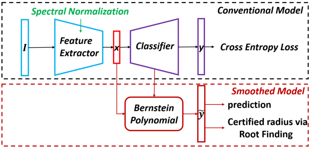
Figure 2: Architecture Design. Top: A typical image classifier specialized in spectral normalization, adding to each layer of a feature extractor. We compress the layer $x$ to a small dimension. Bottom: We adopt Bernstein polynomial to smooth the classifier for prediction and certification.

Proposed Method

In this paper, we concern about “What is a smooth classifier?”. We can think it as a function that can be differentiated infinitely times, and the function we differentiate is still continuous. The simplest example we can think of is polynomials. Hence, we try to approximate a neural network classifier via Bernstein polynomial. Unlike convolution with a Gaussian distribution or other distributions, the exact computation of Bernstein polynomial is more natural to apply.

Our method contains three parts, as illustrated in Figure 2. The first part is the spectral normalization. This mechanism is usually introduced to stably train the discriminator in Generative Adversarial Networks (GANs). Spectral normalization is adopted here because it can make the feature extractor’s output be bounded due to the change of input.

The second part is the Bernstein polynomial approximation, which is the most important one. Bernstein polynomial takes a feature vector and the classifier into consideration (See Equation (7)). We can also consider this form as uniform sampling in $[0,1]^{d}$ and place these samples into the base classifier to obtain the coefficients. With these coefficients, we manage to use a linear combination of Bernstein basis to construct a smoother version of the base classifier. To overcome the computational complexity of high dimensional Bernstein polynomials, we compress $x$ to have small (say 3$\sim$6) dimensions.

The last part is the process of calculating the certified radius via root-finding. We construct nonlinear systems of equations to characterize the points on the decision boundary and solve them by numerical root-finding techniques. After applying this process, we obtain a certified radius for each input data.

Spectral Normalization (SN)

According to (Miyato et al. 2018), spectral normalization controls the Lipschitz constant of neural networks that were originally used in stabilizing the training of the discriminator in GANs. The formulation is stated as:

$$W_{SN}^{(i)}=\frac{W_{i}}{\sigma(W_{i})},\sigma(W_{i})=\max_{x:x\neq 0}\frac{\|W_{i}x\|_{2}}{\|x\|_{2}},$$ (1)

which is equivalent to being divided by the greatest singular value of $W_{i}$, the weights of $i$-th layer. Suppose that our feature extractor $G$ (see Figure 2) is the composition function composed of Lipschitz continuous functions $g_{i}(x^{(i)};W_{SN}^{(i)}):=ReLU(W_{SN}^{(i)}x^{(i)}+b^{(i)})$, where $x^{(i)}$ is the output of $g_{i-1}$ and $b^{(i)}$ is the bias for $i=1,2,\cdots,M$, $i.e.$,

$$G(x^{(1)}):=g_{M}(g_{M-1}\cdots g_{1}(x^{(1)};W_{SN}^{(1)});W_{SN}^{(2)})\cdots;W_{SN}^{(M)}),$$ (2)

where $x^{(1)}=I$ is the input data. For each $g_{i}$ we have

$$\|g_{i}(x^{(i)}+\delta;W_{SN}^{(i)})-g_{i}(x^{(i)};W_{SN}^{(i)})\|_{2}\leq\|W_{SN}^{(i)}\|_{2}\|\delta\|_{2}.$$ (3)

Given two input data $I$ and $I^{\prime}$, and by Equation (1), we have $\|W_{SN}^{(i)}\|_{2}=1$ for $i=1,2,\cdots,M$. We can derive that the Lipschitz constant of $G$ is one by Equation (2) and (3) as:

If $G(I)\neq G(I^{\prime})$, there exists an $R>0$ such that

$$R\leq\|G(I)-G(I^{\prime})\|_{2}\leq\|I-I^{\prime}\|_{2}.$$ (4)

We can further observe from Equation (4) that the upper bound of the certified radius is tighter in feature domain than that in the image domain.

Smoothing the Classifier via Bernstein Polynomial

Weierstrass approximation theorem asserts that a continuous function on a closed and bounded interval can be uniformly approximated on that interval by polynomials to any degree of accuracy. All of the formal definitions are described as follows (Davis 1975).

Theorem 1 (Weierstrass Approximation Theorem).

Let $f\in C([a,b])$. Given $\epsilon>0$, there exists a polynomial $p(x)$ such that

$$|f(x)-p(x)|\leq\epsilon,\hskip 8.61108pt\forall x\in[a,b].$$

Bernstein proved the Weierstrass Approximation theorem in a probability approach (Bernstein 1912). The rationale behind Bernstein polynomial is to compute the expected value $\mathbb{E}[f(\eta/n)]$, where $\eta\sim Bin(n,x)$ and $Bin(n,x)$ is the binomial distribution. Note that the parameter $n$, relating to how it can be used to smooth the classifier, will be elaborated in detail later. The following Definition 1 and Theorem 2 are from (Bernstein 1912).

Definition 1 (Bernstein Polynomial).

Let $f(x)$ be a function defined on $[0,1]$. The $n$-th Bernstein Polynomial is defined by

$$B_{n}(f;x)=\sum\limits_{k=0}^{n}f\left(\frac{k}{n}\right)\binom{n}{k}x^{k}(1-x)^{n-k}.$$ (5)

Note that

$$B_{n}(f;0)=f(0),\hskip 8.61108ptB_{n}(f;1)=f(1).$$

Theorem 2 (Bernstein).

Let $f(x)$ be bounded on $[0,1]$. Then

$$\lim_{n\rightarrow\infty}B_{n}(f;x)=f(x)$$ (6)

at any point $x\in[0,1]$ at which $f$ is continuous. If $f\in C([0,1])$, the limit holds uniformly in $[0,1]$.

Back to Theorem 1, we can take it as a corollary of Theorem 2. Since the neural network is a multi-dimensional function, we have to generalize the one dimensional Bernstein polynomial (Definition 1) into a multi-dimensional version. The following is one kind of generalization which considers independent random variables expectation (Veretennikov and Veretennikova 2016).

Definition 2 ($\bm{d}$-dimensional Bernstein Polynomial).

Let $f:[0,1]^{d}\rightarrow$. We can define $d$-dimensional Bernstein Polynomial by

$$\begin{split}&B_{n_{1},\cdots,n_{d}}(f;x_{1},\cdots,x_{d})\\ &=\sum\limits_{\begin{subarray}{c}0\leq k_{j}\leq n_{j}\\ j\in\{1,\cdots,d\}\end{subarray}}f\left(\frac{k_{1}}{n_{1}},\cdots,\frac{k_{d}}{n_{d}}\right)\prod\limits_{j=1}^{d}\binom{n_{j}}{k_{j}}{x_{j}}^{k_{j}}(1-x_{j})^{n_{j}-k_{j}}.\end{split}$$

For simplicity, we abbreviate the notation by setting $\frac{k}{n}:=\left(\frac{k_{1}}{n_{1}},\cdots,\frac{k_{d}}{n_{d}}\right)$ and $b_{j}:=\binom{n_{j}}{k_{j}}{x_{j}}^{k_{j}}(1-x_{j})^{n_{j}-k_{j}}$, and have

$$B_{n}(f;x)=\sum\limits_{\begin{subarray}{c}0\leq k_{j}\leq n_{j}\\ j\in\{1,\cdots,d\}\end{subarray}}f\left(\frac{k}{n}\right)\prod\limits_{j=1}^{d}b_{j}.$$ (7)

How to Smooth the Classifier via Bernstein Polynomial?

As we can see from Theorem 2, as $n$ becomes larger, the Bernstein polynomial will gradually approximate the original function. Thus, the rationale behind our Bernstein polynomial-based smoothed classifier is that we can choose a proper $n$ to smooth and approximate the base classifier. Obviously, there is a trade-off between smoothness (robustness) and accuracy (natural accuracy). We use an example to visualize Theorem 2 in Figure 3.

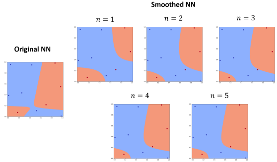
Figure 3: Decision boundaries of the neural network variants under different $n$s. As we can see, the smoothed decision boundary obtained with a larger $n$ gradually approximates the original neural network.

By Definition 2, we can transform our classifier $f:[0,1]^{d}\rightarrow^{K}$, $f=[f_{1},f_{2},\cdots,f_{K}]$, into a smoothed classifier as

$$\tilde{f}(x)=[B_{n}(f_{1};x),\cdots,B_{n}(f_{K};x)],$$ (8)

with a proper choice of $n$.

Without any prior knowledge of the pre-trained neural network, we set $n_{1}=n_{2}=\cdots=n_{d}=n$, which denotes the uniform sampling in all directions. We can see that the complexity of computing $d$-dimensional Bernstein Polynomial is $O(n^{d})$, which is too high in the image domain even if we take $n=2$. To overcome this problem, we propose to exploit dimension reduction in the feature layer. As we will see later in our empirical results, less than $1\%$ natural accuracy will be sacrificed in MNIST (LeCun, Cortes, and Burges 2010) and CIFAR-10 due to dimensionality reduction in the feature space.

Certified Radius via Root-Finding

To find the certified radius of the input data, different from (Cohen, Rosenfeld, and Kolter 2019), we are not trying to find a closed form solution. Instead, we propose to use numerical root-finding techniques to find an adversarial example in the feature domain.

We abbreviate the notation by setting $\beta_{i}=B_{n}(f_{i};x)$ and $S(\beta)_{i}=\exp(\beta_{i})/\sum_{j=1}^{K}\exp(\beta_{j})$, where $K$ is the number of classes. Note that $S(\beta)$ is the traditional softmax function which represents the probability vector. Also, recall that $d\leq K$ is the dimension of a feature vector $x_{0}$.

In the worst case analysis, the runner-up class is the easiest target for attackers. Hence, we assume that the closest point to a feature vector $x_{0}$ on the decision boundary between the top two predictions of the smoothed classifier $\tilde{f}(x)=\beta=[\beta_{1},\cdots,\beta_{K}]$ follows $\beta_{\rho(1)}=\beta_{\rho(2)}$, where $\rho$ is the mapping from ranks to predictions. Therefore, the nonlinear systems of equations for characterizing the points on the decision boundary of smoothed classifier $\tilde{f}(x)$ are described as:

$$\begin{cases}\phi_{0}:=\beta_{\rho(1)}-\beta_{\rho(2)}=0\\ \phi_{1}:=S(\beta)_{\rho(1)}-0.5=0\\ \phi_{2}:=S(\beta)_{\rho(2)}-0.5=0\\ \phi_{3}:=S(\beta)_{\rho(3)}=0\\ \hskip 34.44434pt\vdots\\ \phi_{d}:=S(\beta)_{\rho(d)}=0\\ \end{cases}$$ (9)

where $\phi_{0}$ can be seen as the decision boundary between the top two predictions, and $\phi_{1}$ and $\phi_{2}$ are the probabilities of the top two predictions, respectively. The remaining equations indicate that the probabilities other than $\rho(1)$ and $\rho(2)$ are all zeros. The only thing we need to do is to start from the initial guess (feature vector $x_{0}$) and find the adversary nearest to it.

To solve Equation (9), we transform it into a minimization problem. We consider the function $\Phi:^{d}\rightarrow^{d}$, $\Phi=(\phi_{0},\phi_{1},\cdots,\phi_{d})$, and minimize $\frac{1}{2}\|\Phi(x)\|_{2}^{2}$ is equivalently to finding

$$x^{*}=\operatorname*{arg\,min}_{x}\{F(x)\},$$ (10)

where $F(x)=\frac{1}{2}\sum\limits_{i=0}^{d}(\phi_{i}(x))^{2}=\frac{1}{2}\|\Phi(x)\|_{2}^{2}.$

Suppose that $x^{*}$ is the optimal solution to Equation (9), that is, $\Phi(x^{*})=0$. According Equation (10), we have $F(x^{*})=0$ and $F(x)>0$ if $\Phi(x)\neq 0$. The details of how to solve Equation (10) are described in the Appendix. Let sol denote the solution of Equation (10), we can easily compute $R=\|x_{0}-\emph{sol}\|_{p}$ for $p>1$, which is known as the certified radius. Remark that this radius is computed in the feature domain (see Equation (4)). On the other hand, we prove that our method satisfies the following proposition specialized in norm independence.

Proposition 1.

Let $\tilde{f}:[0,1]^{d}\rightarrow^{K}$ be a smoothed function and $A=\{\tilde{y}\in^{K}:\tilde{y}_{i}\neq\tilde{y}_{j},\forall i\neq j\}$ denote the area without the smoothed decision boundary. For any $x\in[0,1]^{d}$ and $\tilde{f}(x)\in A$, there exists an $R>0$ such that $\operatorname*{arg\,max}_{i\in[K]}\tilde{f_{i}}(x+\hat{\delta})=\operatorname*{arg\,max}_{i\in[K]}\tilde{f_{i}}(x)$ whenever $\|\hat{\delta}\|_{p}<R$  for  $p>1$.

The proof can be found in the Appendix.

Inference procedure

Suppose that we have a pre-trained model for the purpose of either prediction or certification. The prediction is a simple substitution of a smoothed classifier for the base classifier. Hence, we mainly illustrate our smoothing and certification procedures in Algorithm 1 and 2, respectively.

Input: A classifier $f$, a feature $x_{0}$, and a parameter $n$

Output: $\beta(=\tilde{f}(x_{0}))$, the output of the smoothed classifier

Initialize an empty array $\beta=[\hskip 4.30554pt]$;

for i=1,2,$\cdots$, K do

      Compute Equation (7) by $f_{i},x_{0}$ and $n$ to get $\beta_{i}$;

       Append $\beta_{i}$ to $\beta$;

      

end for

return $\beta$

Algorithm 1 Smooth($f$, $x_{0}$, $n$)

Input: An input data $I$, a feature extractor $G$, a classifier $f$, and a parameter $n$

Output: Certified Radius $R$

$x_{0}=G(I)$;

$\beta$ = Smooth($f$, $x_{0}$, $n$);

Setup Equation (9) by $\beta$ and the dimension of $x_{0}$;

Let $x_{0}$ be the initial guess;

Transform Equation (9) into Equation (10);

Solve Equation (10) by a least-squares solver;

Project sol onto $[0,1]^{d}$;

$R=\|x_{0}-\emph{sol}\|_{p}$;

return $R$

Algorithm 2 Certification($I$, $G$, $f$, $n$)

Deterministic algorithm

Note that our deterministic algorithm has two-fold meanings, $i.e.$, deterministic smoothing and deterministic certification. By the definition of the deterministic algorithm, given a particular input, it always produces the same output. Hence, Algorithm 1 and 2 are both deterministic. There are some advantages and disadvantages to the robust classification task. The most significant advantage is that our algorithm does not depend on any random value; it always produces a stable output (robustness). The disadvantage is that for attackers, attacking the smoothed classifier is no more difficult than attacking the non-smoothed classifier since it is end-to-end differentiable. Thus, we do not claim that our method is a defense mechanism but a certification/verification method.

Experiments

In this section, we aim to compare our method with state of the art certification methods, randomized smoothing (Cohen, Rosenfeld, and Kolter 2019) (Salman et al. 2019a), on CIFAR-10. We also compare the empirical upper bound using PGD attack (Madry et al. 2018) with our certified accuracy at all radii. Other results obtained from different datasets such as MNIST, SVHN (Netzer et al. 2011), and CIFAR-100 (Krizhevsky, Hinton et al. 2009) would be discussed in the Appendix. In addition, we perform the ablation study.

Important Metrics

We are interested in three significant metrics, natural accuracy, robust accuracy, and certified accuracy. Natural accuracy is the number of correctly identified clean testing examples divided by the number of total testing examples. Robust accuracy is the number of correctly identified adversarial testing examples divided by the number of total testing examples. Certified accuracy at radius $R$ is defined as the fraction of testing examples correctly predicted by the classifier and are provably robust within an $\ell_{2}$ ball of radius $R$. For brevity, we define the certified accuracies at all radii as “certified curve”.

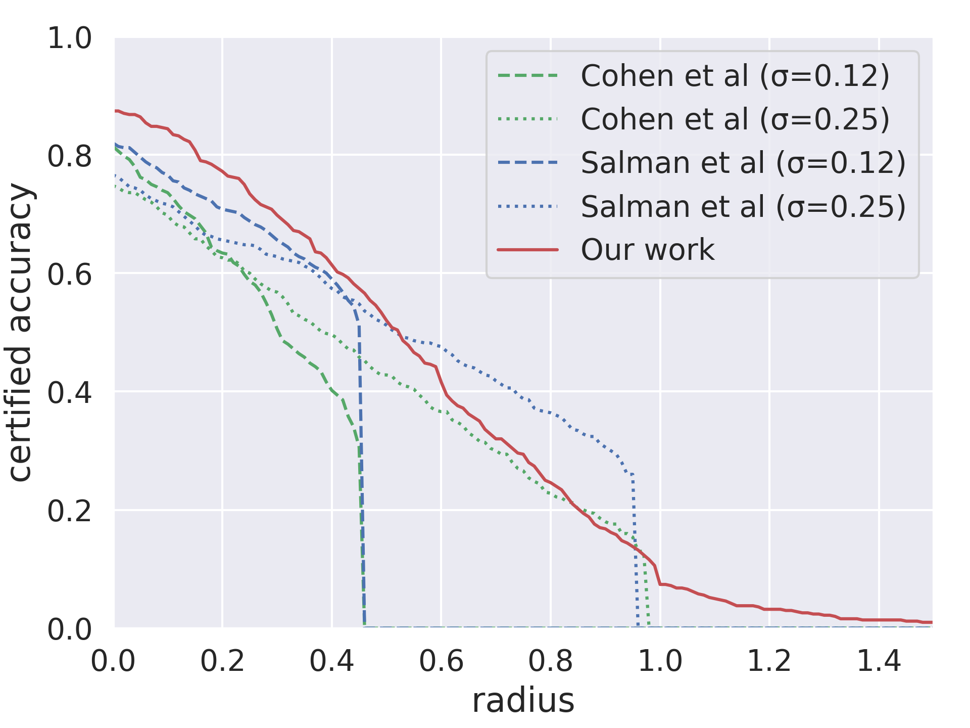
Figure 4: Comparing our adversarially-trained model vs. (Cohen, Rosenfeld, and Kolter 2019) and (Salman et al. 2019a) with $\sigma=0.12$ and $\sigma=0.25$ on CIFAR-10. Our result exhibits the highest natural accuracy under $n=1$ and $d=5$. For fair comparison with their methods, we chose the NN models with the top two natural accuracy (the certified accuracy at radius equals to zero).

Experimental Setup

The architecture of our method is illustrated in Figure 2. We trained the model by adding spectral normalization to every layer of feature extractor $G$ and reducing the feature vector’s dimension to a small number. According to (Salman et al. 2019a), they employ PGD adversarial training to improve the certified curve empirically. Hence, we aslo incorporated it into our model architecture at the expense of decreasing the natural accuracy slightly. As for inference, we applied the reduced feature $d$ to find the exact distance to the decision boundary by using root-finding algorithms from scipy.optimize package (Virtanen et al. 2020). Details of the algorithm we used will be further discussed in the Appendix.

We employed a 110-layer residual network as our base model for a reasonable comparison, which was also adopted in (Cohen, Rosenfeld, and Kolter 2019) and (Salman et al. 2019a). Furthermore, there are two primary hyperparameters: the parameter $n$ and the dimension $d$ of the feature vector, affecting our smoothed model.

Evaluation Results

We certified a subset of 500 examples from the CIFAR-10 test set, as done in (Cohen, Rosenfeld, and Kolter 2019) and (Salman et al. 2019a), that was released on the Github pages. Our method took 6.48 seconds to certify each example on an NVIDIA RTX 2080 Ti with $n=1$, while 15 seconds are required in (Cohen, Rosenfeld, and Kolter 2019) under the same setting.

We primarily compare with (Cohen, Rosenfeld, and Kolter 2019) and (Salman et al. 2019a) as they were shown to outperform all other provable $\ell_{2}$-defenses thoroughly. Recall that our method is norm-independent, as described in Proposition 1, we did the experiment in $\ell_{2}$ norm to compare with their results. As our work claims to maintain high natural accuracy, we utilized $\sigma=0.12$ and $\sigma=0.25$ from (Cohen, Rosenfeld, and Kolter 2019) and (Salman et al. 2019a), which lead to the top two natural accuracy of their results. For (Salman et al. 2019a), we took one of their results: PGD adversarial training with two steps and $\epsilon=64/255$ for comparison since it has the highest natural accuracy among all of their settings. Note that the results are directly taken from their GitHub pages.

Although we added additional components such as spectral normalization (SN) to the base model for training, the natural accuracy only dropped from 93.7% to 93.5%, which nearly carries no harm than adding Gaussian noise for data augmentation. Then, by applying PGD adversarial training with 20 steps and $\|\epsilon\|_{2}=0.1$ to the base model with SN, the accuracy dropped from 93.5% to 87.6%. We call the adversarial trained model “baseline” in Table 1. We applied our method with $n=1$ to the “baseline” model and got 87.4% accuracy, which is the highest accuracy among the methods used for comparison. As shown in Figure 4, we have the following observations for comparison results:

1. Our method obtains a higher natural accuracy at $R=0$.

2. Our method exhibits higher certified accuracies at lower radii ($R<0.5$) but still obtains non-zero accuracies at larger radii ($R>1.0$).

To check the rationality of our theoretical results, the empirical upper bounds of the certified curve obtained from practical attacks (PGD attack) were used for comparison. Although there are some uncertainties in root finding, the default of the sum of squares error and the approximate solution error are set to $1.49\times 10^{-8}$ which is an acceptable error. Therefore, we can observe from Figure 5 that our certification results approximate the empirical upper bounds. The errors caused by spectral normalization and other possible reasons are discussed in the Appendix.

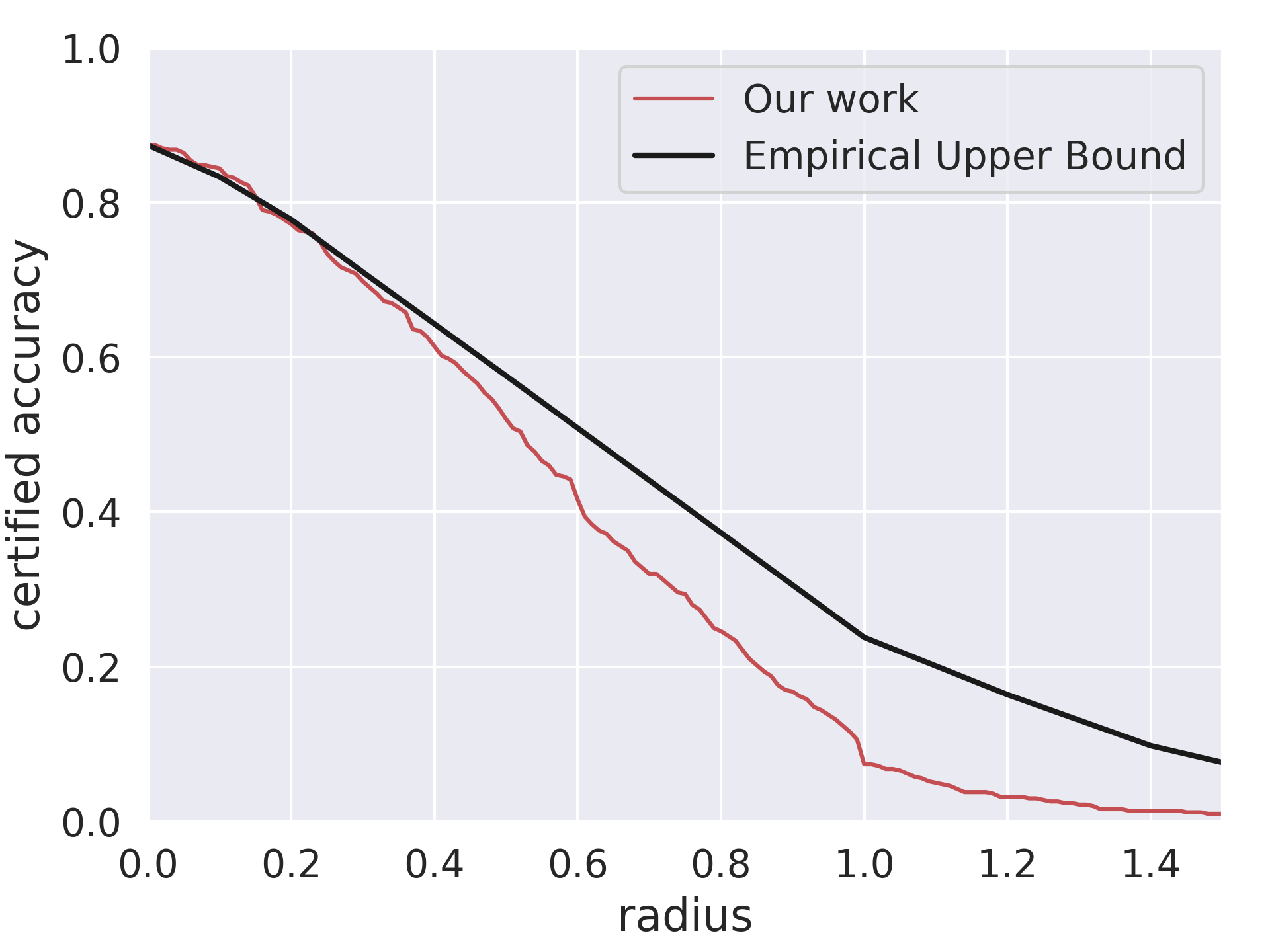
Figure 5: The empirical upper bounds vs. our certified curve on CIFAR-10. The upper bounds are obtained by attacking the smoothed model with $\|\epsilon\|_{2}\in$ {0,0.1,0.2,0.3,0.5,1,1.2,1.4,1.5} via the PGD attack with 20 steps. Our certified curve is relatively conservative, and appears to be beneath the empirical upper bounds.

We can observe from Algorithm 1, where $K$ is the number of the classes of a dataset, $n$ and $d$ are the parameters in Equation (7), the complexity is $O(Kn^{d})$. As $K$ increases, the algorithm may cost an unacceptable time. Therefore, due to the high computational complexity, ImageNet (Deng et al. 2009) was not considered in our results. The scalability of our work would be an interesting issue for future study.

Ablation study

Our method involves some issues, including dimension reduction, different model architectures, and hyperparameters, that may affect the performance. To explore the effectiveness of each part, we conduct ablation studies.

Datasets	Methods	Acc	PGD
CIFAR-10	Baseline	87.6%	63.6%
	Ours with $n=1$	87.4%	63.2%
	Ours with $n=2$	86.8%	63.0%
	Ours with $n=3$	87.2%	62.6%
	Ours with $n=4$	87.4%	62.6%
	Ours with $n=5$	87.4%	62.6%
	Ours with $n=6$	87.4%	63.0%
	Ours with $n=7$	87.4%	63.2%

Table 1: Empirical result comparison between the base classifier and the smoothed classifier. The perturbation of the attacks were set to $\|\epsilon\|_{\infty}=2/255$ in PGD with 20 steps. Acc denotes natural accuracy. Note that CIFAR-10 refers to a subset of 500 examples from the test set.

First, the robust accuracy should be proportional to the certified accuracy theoretically. We conducted an experiment to find $n$ that results in the best robust accuracy. From Table 1, we observe that as $n=1$ and $n=7$, the natural accuracy and the robust accuracy under PGD are the highest among all $n$s. Since our method with $n=1$ spends the lowest computation time, we used $n=1$ in all the other experiments. Remark that our method is a certification instead of a defense method. Thus, as we chose $n=1\sim 7$, natural accuracy and robust accuracy are slightly lower than the baseline. However, we discover an intriguing phenomenon in other datasets and models in that we may have better natural accuracy and robust accuracy than the baseline with a proper choice of $n$ (see Table 4 in the Appendix).

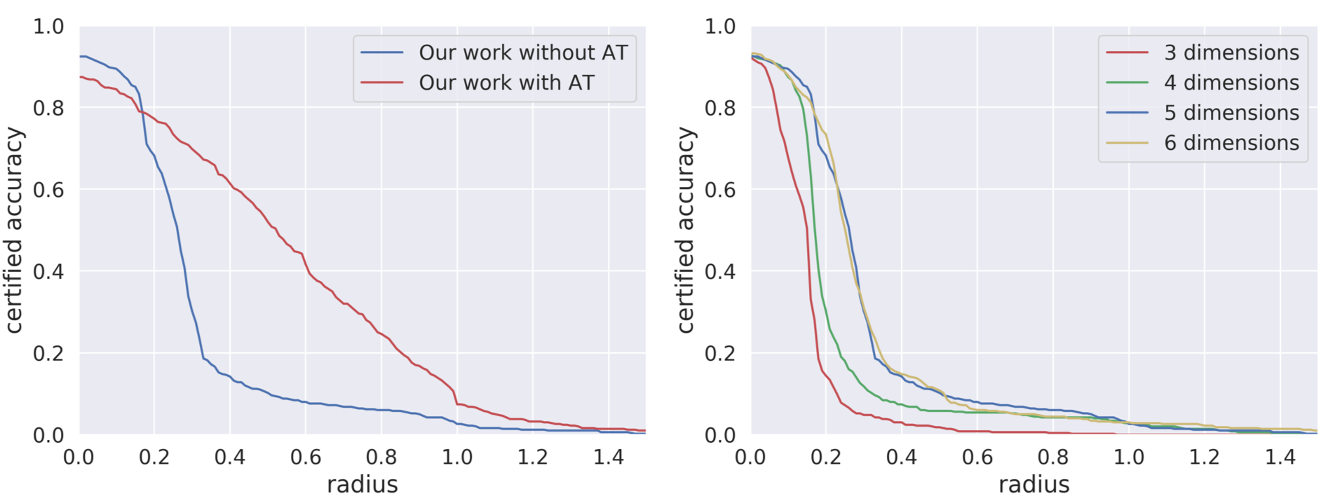
Figure 6: Left: Comparison between our method with and without adversarial training. Right: Certified curve under different dimensions in our non-adversarially trained smoothed classifier. Note that the dimension represents the number of equations we solve to find the root.

Second, on the left side of Figure 6, we show that adversarial training is still a useful heuristic strategy that improves the certified curve while sacrificing only limited natural accuracy at radius = $0$.

In addition, the dimension of the feature vector influences the certified curve a lot. We can observe from the right side of Figure 6 that the feature dimensions of length five and six lead to the best certified curve. However, the larger dimension, the longer the computation time. This is why the feature dimension is set to be five in our experiments. Since our feature domain is constrained in the $[0,1]^{d}$, there is an upper bound of the certified radius, which is the dimension’s square root if we choose $\ell_{2}$ norm.

Finally, we find that most black-box certification methods only exploit one model in their experiments, which is considered insufficient in some cases. Different model architectures may differ a lot in the certified curve. Hence, we employ several models, including ResNet, WideResNet, VGG, and DenseNet, to support our claim. (See Figure 8 in the Appendix.)

Remedy Over-fitting of Regression Model

In a regression problem, one often has a large amount of features. To prevent over-fitting to the training dataset, feature engineering provides a sophisticated design. Most of them are based on statistical tools to select very few representative data. However, it might also not be able to prevent over-fitting and perform worse with respect to unseen data. Our method provides a post-processing step to smooth the original regression model and preserve its shape. Figure  7 shows an example to verify our claim.

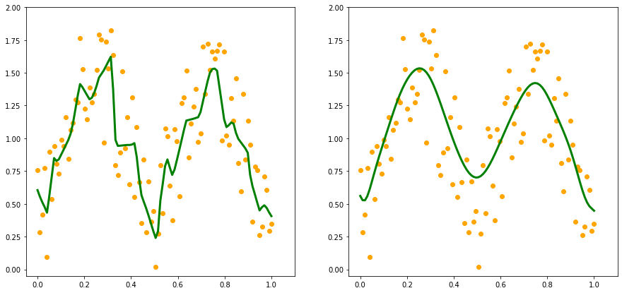
Figure 7: Regression Model. In both graphs, orange dots are noisy training data and green curve denotes the model prediction. Left: The original over-fitting regression model. Right: After applying our method, the shape is smoothed without over-fitting to outliers.

Conclusion and Future Work

We are first to achieve deterministic certification to adversarial attacks via Bernstein polynomial. Moreover, we demonstrate through 2D example visualization, theoretical analyses, and extensive experimentation that our method is a promising research direction for classifier smoothing and robustness certification. Besides smoothing the decision boundary, our method can also be applied to other tasks like over-fitting alleviation. Since the idea “smoothing” is a general regularization technique, it may be beneficial in various machine learning domains.

Appendix A Appendix of Deterministic Certification to Adversarial Attacks via
Bernstein Polynomial Approximation

The appendix is organized as follows. Firstly, we provide a notation table. Secondly, proofs mentioned in the main paper are provided. Thirdly, we offer more experimental results using MNIST, SVHN, and CIFAR-100. Fourthly, we discuss how to solve non-linear systems of equations in detail. Finally, we discuss the certification errors resulted from spectral normalization with skip connections, the singularity of Jacobian matrices, and the conservative constant.

Appendix B Notations

Notation	Definition
$I$	input data
$n$	number of trials
$x=[x_{1},\cdots,x_{d}]^{T}$	feature vector
$x_{i}$, $i=\{1,2,\cdots,d\}$	success probability for each trial
$f:[0,1]^{d}\rightarrow^{K}$	base classifier
$\tilde{f}:[0,1]^{d}\rightarrow^{K}$	smoothed classifier
$G:^{|I|}\rightarrow[0,1]^{d}$	feature extractor
$y\in^{K}$	output vector
$\tilde{y}\in^{K}$	smoothed output vector
$B_{n}(f;x)$	Bernstein polynomial
$C(A;B)$	A set of continuous functions that maps from A to B
$C^{\infty}(A;B)$	A set of smooth functions that maps from A to B
$[K]=\{1,\cdots,K\}$	number of classes
$\rho:[K]\rightarrow[K]$	a mapping from ranks to predictions
$R$	certified radius

Table 2: Notations

Appendix C Proof of Proposition 1

Proposition 1. (also stated in the main manuscript) Let $\tilde{f}:[0,1]^{d}\rightarrow^{K}$ be a smoothed function and let $A=\{\tilde{y}\in^{K}:\tilde{y}_{i}\neq\tilde{y}_{j},\forall i\neq j\}$ denote the area without the smoothed decision boundary. For any $x\in[0,1]^{d}$ and $\tilde{f}(x)\in A$, there exists an $R>0$ such that $\operatorname*{arg\,max}_{i\in[K]}\tilde{f_{i}}(x+\hat{\delta})=\operatorname*{arg\,max}_{i\in[K]}\tilde{f_{i}}(x)$ whenever $\|\hat{\delta}\|_{p}<R$  for  $p>1$.

We can prove a more general case of Proposition 1 due to the smooth condition is unnecessary as follows:

Lemma 1.

Let $f:[0,1]^{d}\rightarrow^{K}$ be a continuous function, let $A=\{y\in^{K}:y_{i}\neq y_{j}\forall i\neq j\}\subset^{K}$, and let $X=\{x\in[0,1]^{d}:f(x)\in A\}\subset[0,1]^{d}$. For any $x\in X$, there exists an $R>0$ such that $\operatorname*{arg\,max}_{i\in[K]}f_{i}(x+\delta)=\operatorname*{arg\,max}_{i\in[K]}f_{i}(x)$ whenever $\|\delta\|_{p}<R$  for  $p>1$.

Proof.

The proof contains two cases. The first case states that $\operatorname*{arg\,max}_{i\in[K]}f_{i}(x+\delta)$ is a set and the second case states that $\operatorname*{arg\,max}_{i\in[K]}f_{i}(x+\delta)\neq\operatorname*{arg\,max}_{i\in[K]}f_{i}(x)$.

Case 1 : Suppose that there exists a $\|\delta\|_{p}<R$, and let $x+\delta=x^{\prime}$ such that $\operatorname*{arg\,max}_{i\in[K]}f_{i}(x^{\prime})$ is a set containing multiple elements. Then $f(x^{\prime})\not\in A\Rightarrow x^{\prime}\not\in X$.

Case 2 : Suppose that there exists a $\|\delta\|_{p}<R$, and let $x+\delta=x^{\prime}$ such that $\operatorname*{arg\,max}_{i\in[K]}f_{i}(x^{\prime})\neq\operatorname*{arg\,max}_{i\in[K]}f_{i}(x)$. Define the distance between $f(x)$ and $f(x^{\prime})$ by $d(f(x),f(x^{\prime}))=r$, there is an open ball $\mathbb{B}(f(x),r)$. By the definition of continuous functions in topological spaces, $i.e.$, for each open set in the codomain, its preimage is an open set in that domain. Thus, $f^{-1}(\mathbb{B}(f(x),r))=\mathbb{B}(x,\delta)$ should be an open subset of $X$. However, there exists some $\delta_{1}<\delta$ such that $x+\delta_{1}\not\in X$. This indicates that $f$ is not continuous on $X$. This is a contradiction.

By the results of Case 1 and Case 2, the lemma follows.

∎

Hence, our method can also be applied to neural networks directly. However, due to the massive amounts of deep neural network parameters, the result may be inaccurate. Besides, as $n$ grows larger or the feature vector’s dimension extends, the certification process will be intractable. Thus, we only solve the problem with small $n$ and small dimensions of the feature vector.

Appendix D Additional Experiments

The datasets we use are summarized in Table 3. Among them, MNIST and CIFAR-10 have been popularly used in this area. Since we do not have the certified results of other methods in other datasets, we only conduct experimental comparison between the base classifier and the smoothed classifier to explore the effect of trials empirically.

Dataset	Image size	Training set size	Testing set size	Classes
CIFAR-100	32x32x3	50K	10K	100
CIFAR-10	32x32x3	50K	10K	10
SVHN	32x32x3	73K	26K	10
MNIST	28x28x1	60K	10K	10

Table 3: The evaluation datasets are sorted based on descending order of image size.

For CIFAR-10

As mentioned before, different model architecture may differ a lot in the certified curve. In Figure 8, we can see that the certified curve varies a lot. For certified radius at 0, the accuracy differs from 89% (Wide ResNet) to 81% (VGG19). As for radius at 0.2, the accuracy also varies in a wide range. Although the tendency of certified curves look similar, their gaps may differ by more than 10%, which is a significant difference.

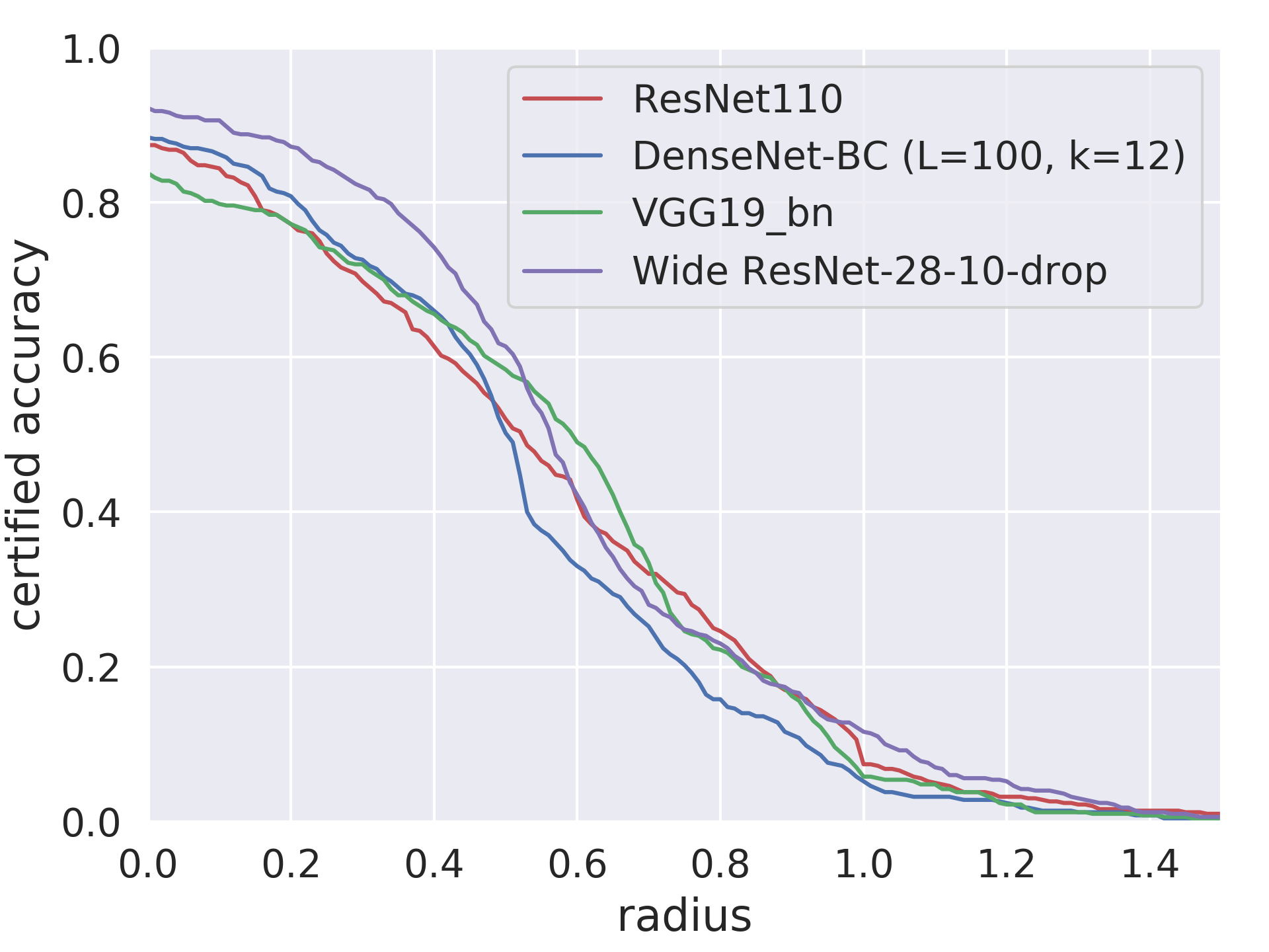
Figure 8: Employing different adversarially trained models to show the certified curve is actually model-dependent.

For MNIST

We include MNIST (LeCun, Cortes, and Burges 2010) to demonstrate some of our claims in a simple manner. As we mentioned in Table 4 of the main paper, if we take $n=5$, the natural accuracy 98.51% and robust accuracy 59.16% in our method are both larger than the baseline with the natural accuracy 98.50% and robust accuracy 52.25%. As we can also see in Figure 9 that there is a trade-off between the number of $n$ and certified accuracy.

Datasets	Methods	Acc	FGSM	PGD
MNIST	Baseline	98.50%	61.46%	52.25%
	Ours with $n=1$	57.09%	43.79%	42.63%
	Ours with $n=2$	77.51%	48.67%	45.99%
	Ours with $n=3$	98.29%	64.37%	61.33%
	Ours with $n=4$	98.45%	64.55%	60.67%
	Ours with $n=5$	98.51%	63.26%	59.16%
	Ours with $n=6$	98.51%	62.82%	58.06%
	Ours with $n=7$	98.50%	61.76%	57.03%

Table 4: (MNIST) Empirical result comparison between the base classifier and the smoothed classifier. Note that $\|\epsilon\|_{\infty}=0.1$ was set for attacks in FGSM and PGD (20 steps). Acc denotes natural accuracy.

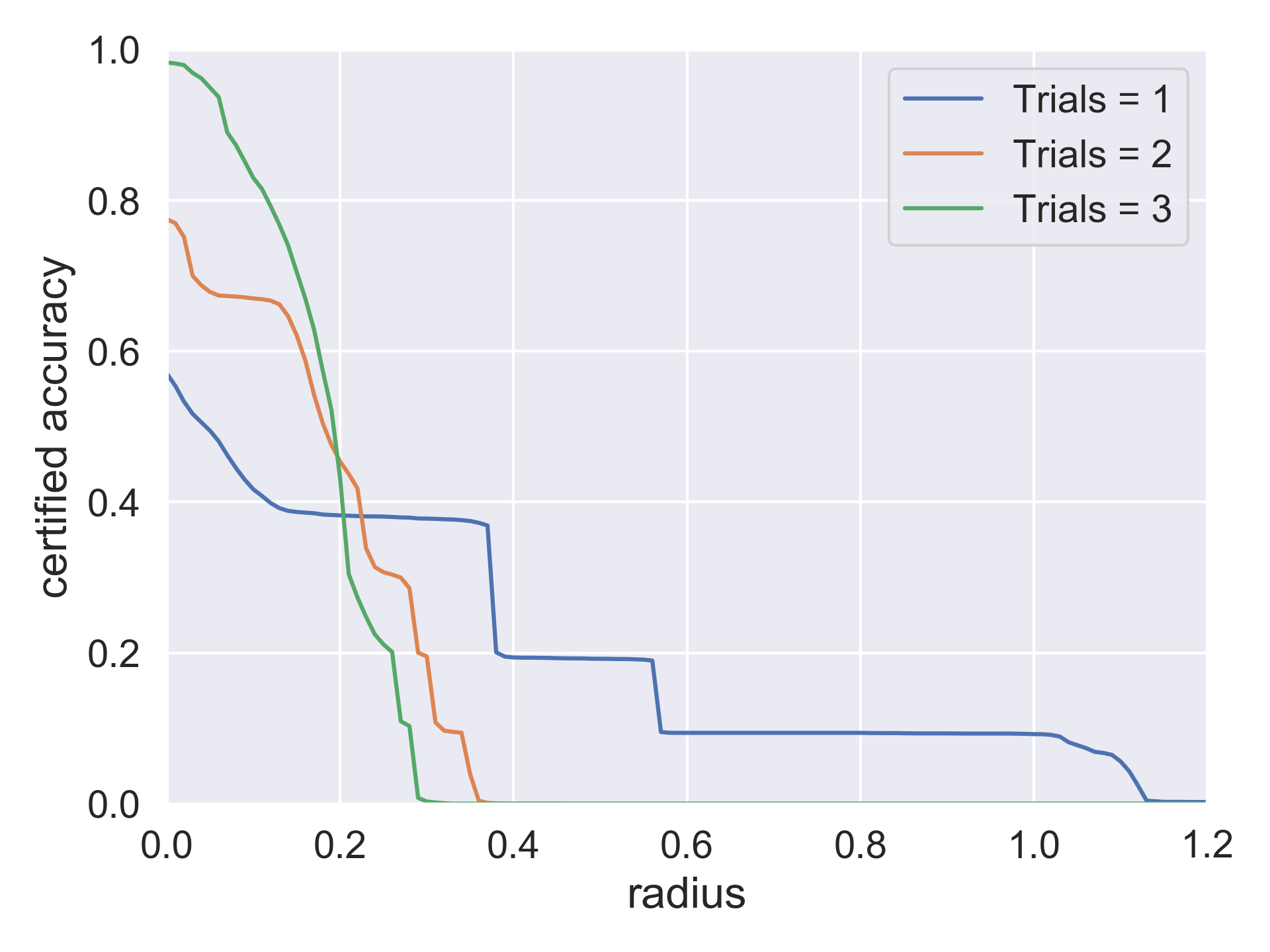
Figure 9: Trade-off between the number of $n$ and certified accuracy (MNIST is taken as an example here. We see similar phenomena in other datasets.) Smaller/larger $n$s exhibit larger/smaller certified radii but suffer from lower/higher natural accuracies.

Datasets	Methods	Acc	FGSM	PGD
SVHN	Baseline	95.07%	56.85%	38.66%
	Ours with $n=1$	78.31%	47.80%	34.60%
	Ours with $n=2$	94.03%	55.80%	39.13%
	Ours with $n=3$	94.59%	56.63%	39.55%
	Ours with $n=4$	94.71%	57.00%	39.42%
	Ours with $n=5$	94.82%	57.28%	39.40%
	Ours with $n=6$	94.88%	57.39%	39.49%
	Ours with $n=7$	94.91%	57.54%	39.48%

Table 5: (SVHN) Empirical result comparison between the base classifier and the smoothed classifier. Note that $\|\epsilon\|_{\infty}=0.01$ was set for attacks in FGSM and PGD with 20 steps. Acc denotes natural accuracy.

Datasets	Methods	Acc	FGSM	PGD
CIFAR100	Baseline	61.6%	33.6%	38.4%
	Ours with $n=1$	33.8%	16.2%	17.4%
	Ours with $n=2$	52.8%	27.8%	31.0%
	Ours with $n=3$	59.0%	32.4%	36.4%
	Ours with $n=4$	59.4%	33.4%	38.4%
	Ours with $n=5$	60.6%	34.2%	38.6%
	Ours with $n=6$	60.0%	33.8%	38.2%

Table 6: (CIFAR-100) Empirical result comparison between the base classifier and the smoothed classifier. Note that $\|\epsilon\|_{\infty}=2/255$ was set for attacks in FGSM and PGD with 20 steps. Acc denotes natural accuracy.

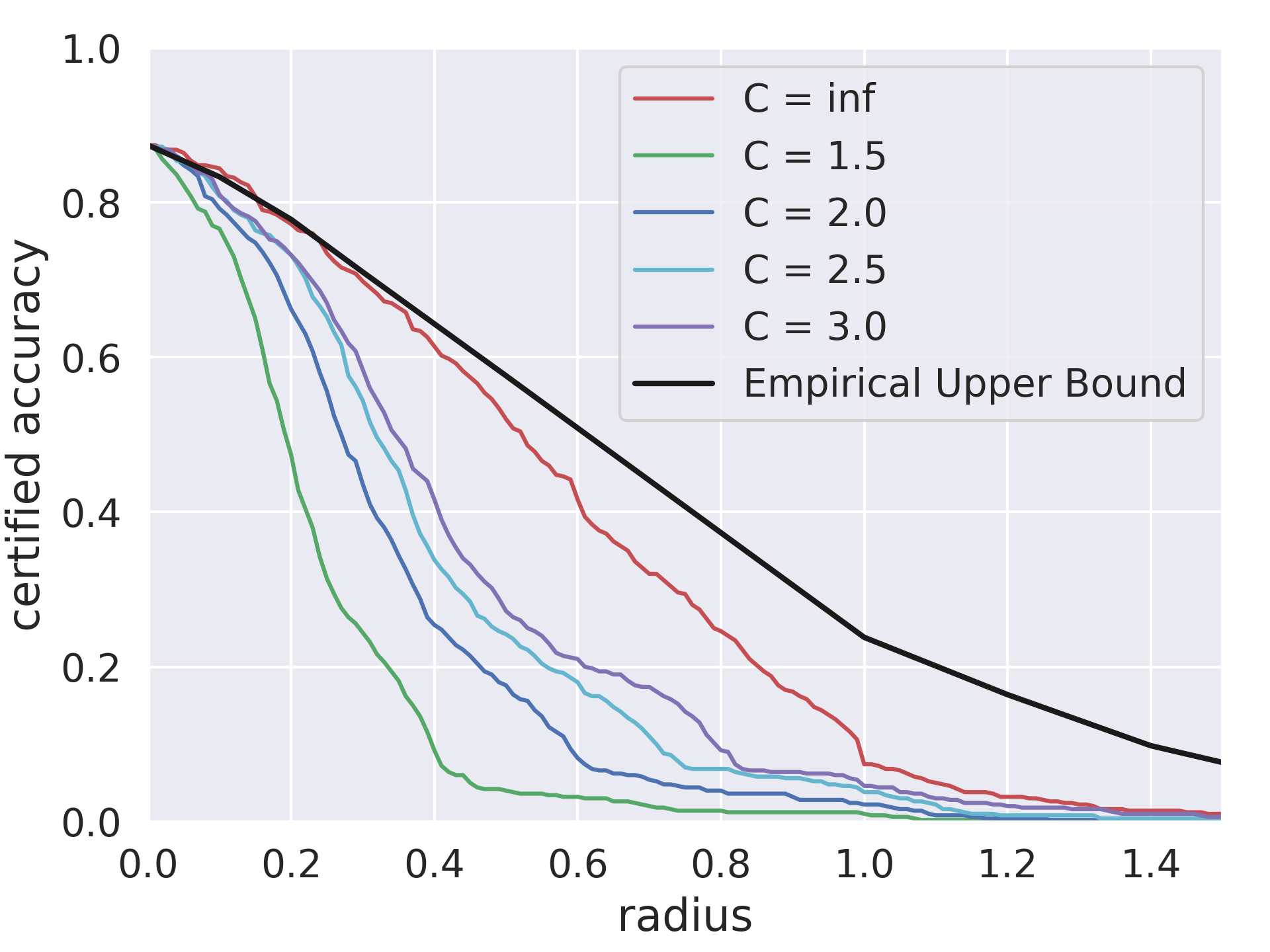
Figure 10: Comparison with different Cs. As C is a conservative parameter, the larger the C is, the closer it is towards the empirical upper bounds.

Appendix E Non-Linear Least Squares Problems and Root-Finding

In Algorithm 2 of the main paper, we adopt a least-square solver. (Madsen, Nielsen, and Tingleff 2004) is a great resource for solving nonlinear least squares problem so we suggest readers to find more details in this book. To make this paper self-contained, we describe some important methods from (Madsen, Nielsen, and Tingleff 2004) below.

First we consider a function $f:^{n}\rightarrow^{m}$ with $m\geq n$. Minimizing $\|f(x)\|$ is equivalent to finding

$$x^{*} =\operatorname*{arg\,min}_{x}\{F(x)\}.$$

$$F(x) =\frac{1}{2}\sum\limits_{i=1}^{m}(f_{i}(x))^{2}=\frac{1}{2}\|f(x)\|^{2}=\frac{1}{2}f(x)^{T}f(x).$$

Let $f\in C^{2}(^{n};^{m})$, and consider Taylor Expansion

$$f(x+h)=f(x)+J(x)h+O(\|h\|^{2}),$$ (11)

where $J(x)\in^{m\times n}$ is the Jacobian matrix, we have $(J(x))_{ij}=\frac{\partial f_{i}}{\partial x_{j}}(x)$. Since $F:^{n}\rightarrow$, we can denote the first derivative and second derivative of $F$, respectively, in Equations (12) (13) and Equations (14) (15) as:

$$\frac{\partial F}{\partial x_{j}} =\sum\limits_{i=1}^{m}f_{i}(x)\frac{\partial f_{i}(x)}{\partial x_{j}}.$$ (12)

$$F^{\prime}(x) =J(x)^{T}f(x).$$ (13)

$$\frac{\partial^{2}F}{\partial x_{j}\partial x_{k}} =\sum\limits_{i=1}^{m}\frac{\partial f_{i}(x)}{\partial x_{j}}\frac{\partial f_{i}(x)}{\partial x_{k}}+f_{i}(x)\frac{\partial f_{i}(x)}{\partial x_{j}\partial x_{k}}.$$ (14)

$$F^{\prime\prime}(x) =J(x)^{T}J(x)+\sum\limits_{i=1}^{m}f_{i}(x)f_{i}^{\prime\prime}(x).$$ (15)

Gradient Descent (Newton-Raphson’s method)

Let $f(x+h)\approx l(h):=f(x)+J(x)h$, which is the first order Taylor expansion. Suppose that we find an $h$ such that $f(x+h)=0$. We have the following iteration form:

$$J(x_{k})h =-f(x_{k})$$ (16)

$$x_{k+1} =x_{k}+h.$$ (17)

Gauss-Newton method

First, we also consider $f(x+h)\approx l(h):=f(x)+J(x)h$ and $F(x+h)\approx L(h)$, where

$$L(h) :=\frac{1}{2}l(h)^{T}l(h),\hskip 21.52771pt(with\ f=f(x)\ and\ J=J(x))$$

$$=\frac{1}{2}[(f^{T}+h^{T}J^{T})(f+Jh)]$$

$$=\frac{1}{2}[f^{T}f+f^{T}Jh+h^{T}J^{T}f+h^{T}J^{T}Jh]$$

$$=\frac{1}{2}f^{T}f+h^{T}J^{T}f+\frac{1}{2}h^{T}J^{T}Jh$$

$$=F(x)+h^{T}J^{T}f+\frac{1}{2}h^{T}J^{T}Jh.$$ (18)

We can further compute the first and second derivative of $L(h)$, respectively, as

$$L^{\prime}(h) =J^{T}f+J^{T}Jh$$ (19)

$$L^{\prime\prime}(h) =J^{T}J.$$ (20)

From Equations (13) and (19), we have $L^{\prime}(0)=F^{\prime}(x)$. If $J$ has full rank, $L^{\prime\prime}(h)$ is positive definite. We have the following iteration form:

$$J^{T}(x_{k})J(x_{k})h_{gn} =-J^{T}(x_{k})f(x_{k})$$ (21)

$$x_{k+1} =x_{k}+\alpha h_{gn}.$$ (22)

Note that $h_{gn}=\operatorname*{arg\,min}\limits_{h}\{L(h)\}$ is called Gauss-Newton step and it is a descent direction since

$$h_{gn}^{T}F^{\prime}(x)=h_{gn}^{T}(J^{T}f)=-h_{gn}^{T}J^{T}Jh_{gn}<0.$$ (23)

Provided that

1. $\{x|F(x)\leq F(x_{0})\}$ is bounded and

2. the Jacobian $J(x)$ has full rank in all steps,

Gauss-Newton method has a convergence guarantee. To overcome the constraint that the Jacobian should have full rank in all steps, the Levenberg–Marquardt method adds a damping parameter $\mu$ to modify Equation (21).

The Levenberg–Marquardt (LM) method

(Levenberg 1944) and (Marquardt 1963) defined the step $h_{lm}$ by modifying Equation (21) as:

$$(J^{T}(x_{k})J(x_{k})+\mu I)h_{lm} =-J^{T}(x_{k})f(x_{k}).$$ (24)

The above modification has lots of benefits; we list some of them as follows:

1. $\forall\mu>0$, $(J^{T}J+\mu I)$ is positive definite which can be proved by the definition of positive definite. This ensures $h_{lm}$ is a descent direction; the proof is similar to Equation (23).

2. For large values of $\mu$, we get $h_{lm}\approx-\frac{1}{\mu}J^{T}f=-\frac{1}{\mu}F^{\prime}(x)$. This is good when $x_{k}$ is far from the solution.

3. If $\mu$ is very small, then $h_{lm}\approx h_{gn}$. This is also a good direction if x is close to the solution $x^{*}$.

We employ Levenberg–Marquardt method (“LM”) (Levenberg 1944) (Marquardt 1963) for $\ell_{2}$ norm certification. The LM method, which is consumed with the advantages of both the Gauss-Newton method and Gradient Descent, is commonly adopted to solve Equation (9).

Trust region method

Recall from Equation (9), we can also add a conservative constant $\xi$ which is similar to the idea of soft margin in the support vector machine. We abbreviate the notation by setting $\beta_{i}=B_{n}(f_{i};x)$ and $S(\beta)_{i}=\exp(\beta_{i})/\sum_{j=1}^{K}\exp(\beta_{j})$, where $K$ is the number of classes. Note that $S(\beta)$ is the traditional softmax function which represents the probability vector. Also, recall that $d\leq K$ is the dimension of a feature vector $x_{0}$.

In the worst case analysis, the runner-up class is the easiest target for attackers. Hence, we assume that the closest point to a feature vector $x_{0}$ on the decision boundary between the top two predictions of the smoothed classifier $\tilde{f}(x)=\beta=[\beta_{1},\cdots,\beta_{K}]$ follows $\beta_{\rho(1)}=\beta_{\rho(2)}$, where $\rho$ is the mapping from ranks to predictions. Therefore, the nonlinear systems of equations for characterizing the points on the decision boundary of $\tilde{f}(x)$ are described as:

$$\begin{cases}\phi_{0}:=\beta_{\rho(1)}-\beta_{\rho(2)}-\xi=0\\ \phi_{1}:=S(\beta)_{\rho(1)}-\frac{1}{1+\exp(-\xi)}=0\\ \phi_{2}:=S(\beta)_{\rho(2)}-\frac{1}{1+\exp(\xi)}=0\\ \phi_{3}:=S(\beta)_{\rho(3)}=0\\ \hskip 34.44434pt\vdots\\ \phi_{d}:=S(\beta)_{\rho(d)}=0\\ \end{cases}$$ (25)

where $\xi=\frac{\beta_{\rho(1)}-\beta_{\rho(2)}}{C}$ is a conservative constant and C is a parameter (see Figure 10). In addition, $\phi_{0}$ can be seen as the decision boundary between the top two predictions if $C\rightarrow\infty$. By $\phi_{0}$, we know that $\beta_{\rho(2)}=\beta_{\rho(1)}-\xi$. We can omit $\beta_{\rho(3)},\cdots,\beta_{\rho(K)}$ since they are too small. By employing softmax function, we have $S(\beta)_{\rho(1)}=\frac{\exp(\beta_{\rho(1)})}{\exp(\beta_{\rho(1)})+\exp(\beta_{\rho(2)})}=\frac{\exp(\beta_{\rho(1)})}{\exp(\beta_{\rho(1)})+\exp(\beta_{\rho(1)}-\xi)}=\frac{1}{1+\exp(-\xi)}$. Also, $S(\beta)_{\rho(2)}$ can be computed in the same way as $S(\beta)_{\rho(1)}$ by setting $\beta_{\rho(1)}=\beta_{\rho(2)}+\xi$. We can observe from $S(\beta)_{\rho(1)}$ and $S(\beta)_{\rho(2)}$ that the probability of top two predictions has a controllable gap $\frac{1}{1+\exp(-\xi)}-\frac{1}{1+\exp(\xi)}$. The remaining equations indicate that the probabilities other than $\rho(1)$ and $\rho(2)$ are all zeros. Equation (25) reveals the decision boundary of the smoothed classifier if $\xi$ is zero, otherwise it represents a margin slightly away from the decision boundary. The only thing we need to do is to start from the initial guess (feature vector $x_{0}$) and find the adversary nearest to it.

We can replace Equation (9) with Equation (25) and solve Equation (10) by means of the trust region method (Nocedal and Wright 2006). First we consider the model function $m_{k}(s_{k})$ by first order Taylor expansion of $\Phi(x_{k}+s_{k})$, that is, $F(x_{k}+s_{k})\approx m_{k}(s_{k})=\frac{1}{2}\|\Phi(x_{k})+J_{k}s_{k}\|_{2}^{2}$. To be precise, $m_{k}(s_{k})$ can be written as:

$$m_{k}(s_{k}) =F(x_{k})+s_{k}^{T}J_{k}^{T}\Phi(x_{k})+\frac{1}{2}s_{k}^{T}B_{k}s_{k}$$ (26)

$$\mathcal{T}_{k} =\{x\in^{n}:\|x-x_{k}\|_{p}\leq\Delta_{k}\},$$ (27)

where $J_{k}=\nabla\Phi(x_{k})$, $B_{k}=J_{k}^{T}J_{k}$ is an approximation of $\nabla^{2}\Phi(x_{k})$, $\mathcal{T}_{k}$ is called the trust region, and $\Delta_{k}$ is the radius of the trust region.

Besides, we need to define a step ratio $r_{k}$ by

$$r_{k} =\frac{F(x_{k})-F(x_{k}+s_{k})}{m_{k}(0)-m_{k}(s_{k})}$$

$$=\frac{\|\Phi(x_{k})\|_{2}^{2}-\|\Phi(x_{k}+s_{k})\|_{2}^{2}}{\|\Phi(x_{k})\|_{2}^{2}-\|\Phi(x_{k})+J_{k}s_{k}\|_{2}^{2}},$$ (28)

where we call the numerator actual reduction and the denominator predicted reduction. $r_{k}$ is used to determine the acceptance or not of the step $s_{k}$ and update (expand or contract) $\Delta_{k}$. Note that the step $s_{k}$ is obtained by minimizing the model $m_{k}$ over the region, including 0. Hence, the predicted reduction is always nonnegative. If $r_{k}$ is negative, then $F(x_{k}+s_{k})$ is greater than $F(x_{k})$ and $s_{k}$ must be rejected. On the other hand, if $r_{k}$ is large, it is safe to expand the trust region.

The trust region method (Nocedal and Wright 2006) is depicted in Algorithm 3. For each iteration, the step $s$ is computed by solving an approximate solution of the following subproblem,

$$\min_{s\in^{n}}m_{k}(s),\hskip 5.0pt\text{subject to}\hskip 2.0pt\|s\|_{p} \leq\Delta_{k},$$ (29)

where $\Delta_{k}$ is the radius of the trust region.

Input: $\hat{\Delta}>0$, $\Delta_{0}\in(0,\hat{\Delta})$ and $\eta\in[0,\frac{1}{4})$

Output: Solution $x_{k}$

for $k=0,1,2\cdots$ do

       Get $s_{k}$ by approximately solving Equation (29);

       Evaluate $r_{k}$ from Equation (E);

       if $r_{k}<\frac{1}{4}$ then

             $\Delta_{k+1}=\frac{1}{4}\Delta_{k}$;

            

      else

             if $r_{k}>\frac{3}{4}$ and $\|s_{k}\|=\Delta_{k}$ then

                  $\Delta_{k+1}=\min(2\Delta_{k},\hat{\Delta})$;

            else

                  $\Delta_{k+1}=\Delta_{k}$;

             end if

            

       end if

      if $r_{k}>\eta$ then

            $x_{k+1}=x_{k}+s_{k}$;

      else

            $x_{k+1}=x_{k}$;

       end if

      

end for

Algorithm 3 Trust region method (Nocedal and Wright 2006)

Due to different $\ell_{p}$ norm, we should change our approach to solve Equation (29). As mentioned in the main paper, we choose LM to solve Equation (29) since the trust region is based on $\ell_{2}$ norm. If we solve Equation (29) in $\ell_{\infty}$ norm, we will adopt the dogbox method (Voglis and Lagaris 2004), which is a modification of the traditional dogleg trust region method (Nocedal and Wright 2006). As for other norms, we can either use the traditional dogleg method with different trust regions or solve the minimization problem by other approaches mentioned in scipy.optimize package.

In the 2D example (see Figure 1), we consider a simpler version of Equation (9), which is $\phi_{0}$, and F(x) becomes $\frac{1}{2}\phi_{0}(x)^{2}$. Recall that our goal is to find a point on the decision boundary which is the closest point to the feature $x_{0}$. Thus, we define the objective function as $\hat{F}(x)=\frac{1}{2}\phi_{0}(x)^{2}+\|x_{0}-x\|^{2}_{2}$, where $\|x_{0}-x\|^{2}_{2}$ is a regularization term, and adopt the trust region method (Nocedal and Wright 2006) to minimize $\hat{F}(x)$. Minimizing $\hat{F}(x)$ is a generalized optimization problem with arbitrary dimensions of $x$. Thus, $-\hat{F}(x)$ can be added to the loss function as a regularization term to fine-tune the model.

The certification procedure (Algorithm 2) is time-consuming as $n$ becomes large. To solve this problem, we can adopt the neural network approach. As (Agrawal et al. 2019) stated, the convex optimization problem is unfolded into a neural network architecture. Hence, we can use the fashion of neural networks to accelerate the certification procedure, which is an interesting future work.

Appendix F The uncertainty of root-finding

Unlike most model architectures contain skip connections, in spectral normalization, we do not consider skip connections. If the feature extractor $G$ contains a skip connection, the Lipschitz constant should be computed by

$$\|G(x)+x-G(x^{\prime})-x^{\prime}\|_{2} <\|G(x)-G(x^{\prime})\|_{2}+\|x-x^{\prime}\|_{2}$$

$$<2\|x-x^{\prime}\|_{2}.$$

If more skip connections are considered, the Lipschitz constant will grow in the power of two. This is a reason why spectral normalization will cause the error. In the training procedure, there might be other ways to control the Lipschitz constant. It is an interesting future work to discuss how to control the Lipschitz constant with skip connections.

Consider Equation (9), we can see that the Jacobian is singular, which is a bad condition for solving minimization problem. In this case, the solution might be inaccurate. However, in practice, we have an acceptable result (see Figure 5) due to the modification of LM (see Equation 24). A better description of the decision boundary is needed to make the Jacobian non-singular which is also an interesting topic to discuss in the future.

The other uncertainty is due to the conservative parameter $\xi=\frac{\beta_{\rho(1)}-\beta_{\rho(2)}}{C}$ in Equation (25). We can observe from Figure 10 that as $C$ gradually grows, the certified curve will approximate the empirical upper bounds. However, in some scenarios, we can only choose small $C$ to make the certified result conservative enough.

References

- Agrawal et al. (2019) Agrawal, A.; Amos, B.; Barratt, S.; Boyd, S.; Diamond, S.; and Kolter, J. Z. 2019. Differentiable convex optimization layers. In Advances in neural information processing systems, 9562–9574.
- Athalye, Carlini, and Wagner (2018) Athalye, A.; Carlini, N.; and Wagner, D. 2018. Obfuscated Gradients Give a False Sense of Security: Circumventing Defenses to Adversarial Examples. In ICML.
- Bernstein (1912) Bernstein, S. 1912. Démo istration du th’eorème de Weierstrass fondée sur le calcul des probabilités. Communications of the Kharkov Mathematical Society 13(1): 1–2.
- Blum et al. (2020) Blum, A.; Dick, T.; Manoj, N.; and Zhang, H. 2020. Random Smoothing Might be Unable to Certify Robustness for High-Dimensional Images. arXiv preprint arXiv:2002.03517 .
- Cao and Gong (2017) Cao, X.; and Gong, N. Z. 2017. Mitigating evasion attacks to deep neural networks via region-based classification. In Proceedings of the 33rd Annual Computer Security Applications Conference.
- Carlini and Wagner (2017a) Carlini, N.; and Wagner, D. 2017a. Adversarial examples are not easily detected: Bypassing ten detection methods. In Proceedings of the 10th ACM Workshop on Artificial Intelligence and Security, 3–14.
- Carlini and Wagner (2017b) Carlini, N.; and Wagner, D. 2017b. Towards evaluating the robustness of neural networks. In 2017 IEEE Symposium on Security and Privacy.
- Cohen, Rosenfeld, and Kolter (2019) Cohen, J.; Rosenfeld, E.; and Kolter, Z. 2019. Certified Adversarial Robustness via Randomized Smoothing. In International Conference on Machine Learning.
- Croce, Andriushchenko, and Hein (2019) Croce, F.; Andriushchenko, M.; and Hein, M. 2019. Provable robustness of relu networks via maximization of linear regions. In the 22nd International Conference on Artificial Intelligence and Statistics.
- Davis (1975) Davis, P. 1975. Interpolation and approximation. Dover books on advanced mathematics. Dover Publications. ISBN 9780486624952.
- Deng et al. (2009) Deng, J.; Dong, W.; Socher, R.; Li, L.-J.; Li, K.; and Fei-Fei, L. 2009. Imagenet: A large-scale hierarchical image database. In CVPR.
- Dvijotham et al. (2018) Dvijotham, K.; Stanforth, R.; Gowal, S.; Mann, T. A.; and Kohli, P. 2018. A Dual Approach to Scalable Verification of Deep Networks. In UAI, volume 1, 2.
- Feinman et al. (2017) Feinman, R.; Curtin, R. R.; Shintre, S.; and Gardner, A. B. 2017. Detecting adversarial samples from artifacts. arXiv preprint arXiv:1703.00410 .
- Feng et al. (2020) Feng, H.; Wu, C.; Chen, G.; Zhang, W.; and Ning, Y. 2020. Regularized Training and Tight Certification for Randomized Smoothed Classifier with Provable Robustness. In The Thirty-Fourth AAAI Conference on Artificial Intelligence. AAAI Press.
- Gehr et al. (2018) Gehr, T.; Mirman, M.; Drachsler-Cohen, D.; Tsankov, P.; Chaudhuri, S.; and Vechev, M. 2018. Ai2: Safety and robustness certification of neural networks with abstract interpretation. In 2018 IEEE Symposium on Security and Privacy.
- Ghiasi, Shafahi, and Goldstein (2020) Ghiasi, A.; Shafahi, A.; and Goldstein, T. 2020. Breaking certified defenses: Semantic adversarial examples with spoofed robustness certificates. In ICLR.
- Goodfellow, Shlens, and Szegedy (2015) Goodfellow, I. J.; Shlens, J.; and Szegedy, C. 2015. Explaining and Harnessing Adversarial Examples. In Bengio, Y.; and LeCun, Y., eds., ICLR.
- Gowal et al. (2018) Gowal, S.; Dvijotham, K.; Stanforth, R.; Bunel, R.; Qin, C.; Uesato, J.; Arandjelovic, R.; Mann, T.; and Kohli, P. 2018. On the effectiveness of interval bound propagation for training verifiably robust models. arXiv preprint arXiv:1810.12715 .
- Katz et al. (2017a) Katz, G.; Barrett, C.; Dill, D. L.; Julian, K.; and Kochenderfer, M. J. 2017a. Reluplex: An efficient SMT solver for verifying deep neural networks. In International Conference on Computer Aided Verification. Springer.
- Katz et al. (2017b) Katz, G.; Barrett, C.; Dill, D. L.; Julian, K.; and Kochenderfer, M. J. 2017b. Towards proving the adversarial robustness of deep neural networks. arXiv preprint arXiv:1709.02802 .
- Krizhevsky, Hinton et al. (2009) Krizhevsky, A.; Hinton, G.; et al. 2009. Learning multiple layers of features from tiny images. Technical Report .
- Kumar et al. (2020) Kumar, A.; Levine, A.; Goldstein, T.; and Feizi, S. 2020. Curse of dimensionality on randomized smoothing for certifiable robustness. arXiv preprint arXiv:2002.03239 .
- Kurakin, Goodfellow, and Bengio (2017) Kurakin, A.; Goodfellow, I. J.; and Bengio, S. 2017. Adversarial Machine Learning at Scale. In ICLR.
- LeCun, Cortes, and Burges (2010) LeCun, Y.; Cortes, C.; and Burges, C. 2010. MNIST handwritten digit database. ATT Labs [Online]. Available: http://yann.lecun.com/exdb/mnist 2.
- Lecuyer et al. (2019) Lecuyer, M.; Atlidakis, V.; Geambasu, R.; Hsu, D.; and Jana, S. 2019. Certified robustness to adversarial examples with differential privacy. In 2019 IEEE Symposium on Security and Privacy.
- Levenberg (1944) Levenberg, K. 1944. A method for the solution of certain non-linear problems in least squares. Quarterly of applied mathematics 2(2).
- Li et al. (2019) Li, B.; Chen, C.; Wang, W.; and Carin, L. 2019. Certified Adversarial Robustness with Additive Noise. In Advances in Neural Information Processing Systems.
- Liao et al. (2018) Liao, F.; Liang, M.; Dong, Y.; Pang, T.; Hu, X.; and Zhu, J. 2018. Defense against adversarial attacks using high-level representation guided denoiser. In CVPR.
- Liu et al. (2018) Liu, X.; Cheng, M.; Zhang, H.; and Hsieh, C.-J. 2018. Towards robust neural networks via random self-ensemble. In Proceedings of the European Conference on Computer Vision (ECCV).
- Ma et al. (2018) Ma, X.; Li, B.; Wang, Y.; Erfani, S. M.; Wijewickrema, S.; Schoenebeck, G.; Houle, M. E.; Song, D.; and Bailey, J. 2018. Characterizing Adversarial Subspaces Using Local Intrinsic Dimensionality. In ICLR.
- Madry et al. (2018) Madry, A.; Makelov, A.; Schmidt, L.; Tsipras, D.; and Vladu, A. 2018. Towards Deep Learning Models Resistant to Adversarial Attacks. In ICLR.
- Madsen, Nielsen, and Tingleff (2004) Madsen, K.; Nielsen, H.; and Tingleff, O. 2004. Methods for Non-Linear Least Squares Problems (2nd ed.). Informatics and Mathematical Modelling, Technical University of Denmark,DTU.
- Marquardt (1963) Marquardt, D. W. 1963. An algorithm for least-squares estimation of nonlinear parameters. Journal of the society for Industrial and Applied Mathematics 11(2).
- Mirman, Gehr, and Vechev (2018) Mirman, M.; Gehr, T.; and Vechev, M. 2018. Differentiable abstract interpretation for provably robust neural networks. In International Conference on Machine Learning.
- Miyato et al. (2018) Miyato, T.; Kataoka, T.; Koyama, M.; and Yoshida, Y. 2018. Spectral Normalization for Generative Adversarial Networks. In ICLR.
- Moosavi-Dezfooli, Fawzi, and Frossard (2016) Moosavi-Dezfooli, S.-M.; Fawzi, A.; and Frossard, P. 2016. Deepfool: a simple and accurate method to fool deep neural networks. In CVPR.
- Netzer et al. (2011) Netzer, Y.; Wang, T.; Coates, A.; Bissacco, A.; Wu, B.; and Ng, A. Y. 2011. Reading digits in natural images with unsupervised feature learning. In NIPS Workshop on Deep Learning and Unsupervised Feature Learning.
- Nocedal and Wright (2006) Nocedal, J.; and Wright, S. 2006. Numerical Optimization. Springer Series in Operations Research and Financial Engineering. Springer New York. ISBN 9780387400655.
- Papernot et al. (2016) Papernot, N.; McDaniel, P.; Jha, S.; Fredrikson, M.; Celik, Z. B.; and Swami, A. 2016. The limitations of deep learning in adversarial settings. In EuroS&P.
- Raghunathan, Steinhardt, and Liang (2018a) Raghunathan, A.; Steinhardt, J.; and Liang, P. 2018a. Certified Defenses against Adversarial Examples. In ICLR.
- Raghunathan, Steinhardt, and Liang (2018b) Raghunathan, A.; Steinhardt, J.; and Liang, P. S. 2018b. Semidefinite relaxations for certifying robustness to adversarial examples. In Advances in Neural Information Processing Systems.
- Salman et al. (2019a) Salman, H.; Li, J.; Razenshteyn, I.; Zhang, P.; Zhang, H.; Bubeck, S.; and Yang, G. 2019a. Provably robust deep learning via adversarially trained smoothed classifiers. In Advances in Neural Information Processing Systems.
- Salman et al. (2019b) Salman, H.; Yang, G.; Zhang, H.; Hsieh, C.-J.; and Zhang, P. 2019b. A convex relaxation barrier to tight robustness verification of neural networks. In Advances in Neural Information Processing Systems, 9835–9846.
- Singh et al. (2018) Singh, G.; Gehr, T.; Mirman, M.; Püschel, M.; and Vechev, M. 2018. Fast and effective robustness certification. In Advances in Neural Information Processing Systems.
- Szegedy et al. (2014) Szegedy, C.; Zaremba, W.; Sutskever, I.; Bruna, J.; Erhan, D.; Goodfellow, I. J.; and Fergus, R. 2014. Intriguing properties of neural networks. In Bengio, Y.; and LeCun, Y., eds., ICLR 2014.
- Tjeng, Xiao, and Tedrake (2019) Tjeng, V.; Xiao, K. Y.; and Tedrake, R. 2019. Evaluating Robustness of Neural Networks with Mixed Integer Programming. In ICLR.
- Tramèr et al. (2018) Tramèr, F.; Kurakin, A.; Papernot, N.; Goodfellow, I.; Boneh, D.; and McDaniel, P. 2018. Ensemble Adversarial Training: Attacks and Defenses. In ICLR.
- Veretennikov and Veretennikova (2016) Veretennikov, A. Y.; and Veretennikova, E. 2016. On partial derivatives of multivariate Bernstein polynomials. Siberian Advances in Mathematics 26(4): 294–305.
- Virtanen et al. (2020) Virtanen, P.; Gommers, R.; Oliphant, T. E.; Haberland, M.; Reddy, T.; Cournapeau, D.; Burovski, E.; Peterson, P.; Weckesser, W.; Bright, J.; van der Walt, S. J.; Brett, M.; Wilson, J.; Jarrod Millman, K.; Mayorov, N.; Nelson, A. R. J.; Jones, E.; Kern, R.; Larson, E.; Carey, C.; Polat, İ.; Feng, Y.; Moore, E. W.; Vand erPlas, J.; Laxalde, D.; Perktold, J.; Cimrman, R.; Henriksen, I.; Quintero, E. A.; Harris, C. R.; Archibald, A. M.; Ribeiro, A. H.; Pedregosa, F.; van Mulbregt, P.; and Contributors, S. . . 2020. SciPy 1.0: Fundamental Algorithms for Scientific Computing in Python. Nature Methods 17: 261–272.
- Voglis and Lagaris (2004) Voglis, C.; and Lagaris, I. 2004. A rectangular trust region dogleg approach for unconstrained and bound constrained nonlinear optimization. In WSEAS International Conference on Applied Mathematics, 7.
- Wang et al. (2018a) Wang, S.; Chen, Y.; Abdou, A.; and Jana, S. 2018a. Mixtrain: Scalable training of formally robust neural networks. arXiv preprint arXiv:1811.02625 14.
- Wang et al. (2018b) Wang, S.; Pei, K.; Whitehouse, J.; Yang, J.; and Jana, S. 2018b. Efficient formal safety analysis of neural networks. In Advances in Neural Information Processing Systems.
- Weng et al. (2018) Weng, L.; Zhang, H.; Chen, H.; Song, Z.; Hsieh, C.-J.; Daniel, L.; Boning, D.; and Dhillon, I. 2018. Towards Fast Computation of Certified Robustness for ReLU Networks. In Proceedings of the 35th International Conference on Machine Learning.
- Wong and Kolter (2018) Wong, E.; and Kolter, Z. 2018. Provable Defenses against Adversarial Examples via the Convex Outer Adversarial Polytope. In Proceedings of the 35th International Conference on Machine Learning, 5286–5295.
- Wong et al. (2018) Wong, E.; Schmidt, F.; Metzen, J. H.; and Kolter, J. Z. 2018. Scaling provable adversarial defenses. In Advances in Neural Information Processing Systems, 8400–8409.
- Xie et al. (2019) Xie, C.; Wu, Y.; Maaten, L. v. d.; Yuille, A. L.; and He, K. 2019. Feature denoising for improving adversarial robustness. In CVPR.
- Xu, Evans, and Qi (2018) Xu, W.; Evans, D.; and Qi, Y. 2018. Feature Squeezing: Detecting Adversarial Examples in Deep Neural Networks. In 25th Annual Network and Distributed System Security Symposium, NDSS 2018, San Diego, California, USA, February 18-21, 2018. The Internet Society.
- Yuan et al. (2019) Yuan, X.; He, P.; Zhu, Q.; and Li, X. 2019. Adversarial examples: Attacks and defenses for deep learning. IEEE transactions on neural networks and learning systems 30(9).
- Zhai et al. (2020) Zhai, R.; Dan, C.; He, D.; Zhang, H.; Gong, B.; Ravikumar, P.; Hsieh, C.-J.; and Wang, L. 2020. MACER: Attack-free and Scalable Robust Training via Maximizing Certified Radius. In ICLR.
- Zhang et al. (2018) Zhang, H.; Weng, T.-W.; Chen, P.-Y.; Hsieh, C.-J.; and Daniel, L. 2018. Efficient neural network robustness certification with general activation functions. In Advances in neural information processing systems.