FreezeNet: Full Performance by Reduced Storage Costs

Abstract

Pruning generates sparse networks by setting parameters to zero. In this work we improve one-shot pruning methods, applied before training, without adding any additional storage costs while preserving the sparse gradient computations. The main difference to pruning is that we do not sparsify the network’s weights but learn just a few key parameters and keep the other ones fixed at their random initialized value. This mechanism is called freezing the parameters. Those frozen weights can be stored efficiently with a single $32$bit random seed number. The parameters to be frozen are determined one-shot by a single for- and backward pass applied before training starts. We call the introduced method FreezeNet. In our experiments we show that FreezeNets achieve good results, especially for extreme freezing rates. Freezing weights preserves the gradient flow throughout the network and consequently, FreezeNets train better and have an increased capacity compared to their pruned counterparts. On the classification tasks MNIST and CIFAR-$10$/$100$ we outperform SNIP, in this setting the best reported one-shot pruning method, applied before training. On MNIST, FreezeNet achieves $99.2\%$ performance of the baseline LeNet-$5$-Caffe architecture, while compressing the number of trained and stored parameters by a factor of $\times 157$.

Backpropagation

1 Introduction

Between $2012$ and $2018$, computations required for deep learning research have been increased by estimated $300,000$ times which corresponds to doubling the amount of computations every few months [36]. This rate outruns by far the predicted one by Moore’s Law [18]. Thus, it is important to reduce computational costs and memory requirements for deep learning while preserving or even improving the status quo regarding performance [36].

Model compression lowers storage costs, speeds up inference after training by reducing the number of computations, or accelerates the training which uses less energy. A method combining these factors is network pruning. To follow the call for more sustainability and efficiency in deep learning we improve the best reported pruning method applied before training, SNIP ([29] Single-shot Network Pruning based on Connection Sensitivity), by freezing the parameters instead of setting them to zero.

SNIP finds the most dominant weights in a neural network with a single for- and backward pass, performed once before training starts and immediately prunes the other, less important weights. Hence it is a one-shot pruning method, applied before training. By one-shot pruning we mean pruning in a single step, not iteratively. This leads to sparse gradient computations during training. But if too many parameters are pruned, SNIP networks are not able to train well due to a weak flow of the gradient through the network [39]. In this work we use a SNIP related method for finding the most influential weights in a deep neural network (DNN). We do not follow the common pruning procedure of setting weights to zero, but keep the remaining parameters fixed as initialized which we call freezing, schematically shown in Figure 1. A proper gradient flow throughout the network can be ensured with help of the frozen parameters, even for a small number of trained parameters. The frozen weights also increase the network’s expressiveness, without adding any gradient computations — compared to pruned networks. All frozen weights can be stored with a single random seed number. We call these partly frozen DNNs FreezeNets.

./tikz/tikz_pic

Figure 1: Graphical illustration of FreezeNet and comparison with a standard neural network (NN) for a fully connected NN with neurons $x_{1},x_{2},x_{3}$ and $y_{1},y_{2}$, and corresponding weights and gradient values. Best viewed in colour.

1.1 Contributions of this Paper and Applications

In this work we introduce FreezeNets, which can be applied to any baseline neural network. The key contributions of FreezeNets are:

• Smaller trainable parameter count than one-shot pruning (SNIP), but better results.

• Preservation of gradient flow, even for a small number of trained parameters.

• Efficient way to store frozen weights with a single random seed number.

• More efficient training than the baseline architecture since the same number of gradients as for pruned networks has to be computed.

Theoretically and empirically, we show that a faithful gradient flow, even for a few trainable parameters, can be preserved by using frozen weights. Whereas pruning weights eventually leads to vanishing gradients. By applying weight decay also on the frozen parameters, we modify FreezeNets to generate sparse networks at the end of training. For freezing rates on which SNIP performs well, this modified training generates networks with the same number of non-zero weights as SNIP while reaching better performances.

Due to their sparse gradient computations, FreezeNets are perfectly suitable for applications with a train-inference ratio biased towards training. Especially for research, where networks are trained for a long time and often validated exactly once, FreezeNets provide a good trade-off between reducing training resources and keeping performance. Other applications for FreezeNets are networks that have to be retrained many times due to changing data, as online learning or transfer learning. Since FreezeNets can reduce the number of stored parameters drastically, they are networks cheap to transfer. This could be of interest for autonomous vehicle fleets or internet services. For a given hardware, FreezeNets can be used to increase the size of the largest trainable network since less storage and computations are needed for applying gradient descent.

2 Related Work

2.1 Network Pruning

Pruning methods are used to reduce the amount of parameters in a network [19, 28, 31]. At the same time, the pruned network should perform equally well, or even better, than the reference network. Speeding up training can be achieved by pruning the network at the beginning of training [29] or at early training steps [12, 13]. There are several approaches to prune neural networks. One is penalizing non-zero weights [3, 4, 20] and thus achieving sparse networks. Nowadays, a more common way is given by using magnitude based pruning [12, 13, 17, 19], leading to pruning early on in training [12, 13], on-the-fly during training [17] or at the end of it [19]. These pruned networks have to be fine-tuned afterwards. For high pruning rates, magnitude based pruning works better if this procedure is done iteratively [12, 13], therefore leading to many train-prune(-retrain) cycles. Pruning can also be achieved by using neural architecture search [10, 22] or adding computationally cheap branches to predict sparse locations in feature maps [9]. The final pruning strategy we want to present is saliency based pruning. In saliency based pruning, the significance of weights is measured with the Hessian of the loss [28], or the sensitivity of the loss with respect to inclusion/exclusion of each weight [25]. This idea of measuring the effect of inclusion/exclusion of weights was resumed in [29], where a differentiable approximation of this criterion was introduced, the SNIP method. Since SNIP’s pruning step is applicable with a single for- and backward pass one-shot before training, its computational overload is negligible. The GraSP (Gradient Signal Preservation) [39] method is also a pruning mechanism, applied one-shot before training. Contrarily to SNIP, they keep the weights possessing the best gradient flow at initialization. For high pruning rates, they achieve better results than SNIP but are outperformed by SNIP for moderate ones.

Dynamic sparse training is a strategy to train pruned networks, but give the sparse architecture a chance to change dynamically during training. Therefore, pruning- and regrowing steps have to be done during the whole training process. The weights to be regrown are determined by random processes [2, 30, 41], their magnitude [40] or saliency [7, 8]. An example of the latter strategy is Sparse Momentum [7], measuring saliencies via exponentially smoothed gradients. Global Sparse Momentum [8] uses a related idea to FreezeNet by not pruning the untrained weights. But the set of trainable weights can change and the untrained weights are not updated via gradient descent, but with a momentum parameter based on earlier updates. Whereas FreezeNet freezes weights and uses a fixed architecture, thus needs to gauge the best sparse network for all phases of training.

In pruning, the untrained parameters are set to $0$ which is not done for FreezeNets, where these parameters are frozen and used to increase the descriptive power of the network. This clearly separates our freezing approach from pruning methods.

2.2 CNNs with Random Weights

The idea of fixing randomly initialized weights in Convolutional Neural Networks (CNNs) was researched in [24], where the authors showed that randomly initialized convolutional filters act orientation selective. In [35] it was shown that randomly initialized CNNs with pooling layers can act inherently frequency selective. Ramanujan et al. [33] showed that in a large randomly initialized base network ResNet$50$ [21] a smaller, untrained subnetwork is hidden that matches the performance of a ResNet$34$ [21] trained on ImageNet [6]. Recently, Frankle et al. [14] published an investigation of CNNs with only Batch Normalization [23] parameters trainable. In contrast to their work, we also train biases and chosen weight parameters and reach competitive results with FreezeNets.

A follow-up work of the Lottery Ticket Hypothesis [12] deals with the question of why iterative magnitude based pruning works so well [42]. Among others, they also investigate resetting pruned weights to their initial values and keeping them fix. The unpruned parameters are reset to their initial values as well and trained again. This train-prune-retrain cycle is continued until the target rate of fixed parameters is reached. In their experiments they show that this procedure mostly leads to worse results than standard iterative pruning and just outperforms it for extremely high pruning rates.

3 FreezeNets

3.0.1 General Setup

Let $f_{\Theta}:\mathbb{R}^{d_{0}}\rightarrow[0,1]^{c}$ be a DNN with parameters $\Theta\subset\mathbb{R}$, used for an image classification task with $c$ classes. We assume a train set $(X,Z)$ with images ${X=\{x_{1},\ldots,x_{N}\}\subset\mathbb{R}^{d_{0}}}$ and corresponding labels $Z=\{z_{1},\ldots,z_{N}\}\subset\{0,1,\ldots,c-1\}$, a test set $(X_{0},Z_{0})$ and a smooth loss function $L$ to be given. As common for DNNs, the test error is minimized by training the network with help of the training data via stochastic gradient based (SGD) optimization [34] while preventing the network to overfit on the training data.

We define the rate $q:=1-p$ as the networks freezing rate, where $p$ is the rate of trainable weights. A high freezing rate corresponds to few trainable parameters and therefore sparse gradients, whereas a low freezing rate corresponds to many trainable parameters. Freezing is compared to pruning in Section 4. For simplicity, a freezing rate $q$ for pruning a network means exactly that $q\cdot 100\%$ of its weights are set to zero. In this work we split the model’s parameters into weights $W$ and biases $B$, only freeze parts of the weights $W$ and keep all biases trainable.

3.1 SNIP

Since pruned networks are constraint on using only parts of their weights, those weights should be chosen as the most influential ones for the given task. Let ${\Theta=W\cup B}$ be the network’s parameters and $m\in\{0,1\}^{|W|}$ be a mask that shows if a weight is activated or not. Therefore, the weights that actually contribute to the network’s performance are given by $m\odot W$. Here $\odot$ denotes the Hadamard product [5]. The trick used in [29] is to look at the saliency score

$$g:=\left.\frac{\partial L(m\odot W;B,X,Z)}{\partial m}\right|_{m=1}=\frac{\partial L(W;B,X,Z)}{\partial W}\odot W\text{\;},$$ (1)

which calculates componentwise the influence of the loss function’s change by a small variation of the associated weight’s activation. If those changes are big, keeping the corresponding weight is likely to have a greater effect in minimizing the loss function than keeping a weight with a small score. The gradient $g$ can be approximated with just a single forward and backward pass of one training batch before the beginning of training.

3.2 Backpropagation in Neural Networks

To simplify the backpropagation formulas, we will deal with a feed-forward, fully connected neural network. Similar equations hold for convolutional layers [21]. Let the input of the network be given by $x^{(0)}\in\mathbb{R}^{d_{0}}$, the weight matrices are given by $W^{(k)}\in\mathbb{R}^{d_{k}\times d_{k-1}}$, $k\in\{1,\ldots,K\}$ and the forward propagation rules are inductively defined as

• $y^{(k)}:=W^{(k)}x^{(k-1)}+b^{(k)}$ for the layers bias $b^{(k)}\in\mathbb{R}^{d_{k}}$ ,

• $x^{(k)}:=\Phi_{(k)}(y^{(k)})$ for the layers non-linearity $\Phi_{(k)}:\mathbb{R}\rightarrow\mathbb{R}$, applied component-wise.

This leads to the partial derivatives used for the backward pass, written compactly in vector or matrix form:

$$\begin{aligned} \frac{\partial L}{\partial y^{(k)}}&=\Phi_{(k)}^{\prime}\left(y^{(k)}\right)\odot\frac{\partial L}{\partial x^{(k)}}\;,&\frac{\partial L}{\partial x^{(k)}}&=\left(W^{(k+1)}\right)^{T}\cdot\frac{\partial L}{\partial y^{(k+1)}}\;,\\ \frac{\partial L}{\partial W^{(k)}}&=\frac{\partial L}{\partial y^{(k)}}\cdot\left(x^{(k-1)}\right)^{T}\;,&\frac{\partial L}{\partial b^{(k)}}&=\frac{\partial L}{\partial y^{(k)}}\end{aligned}\;.$$ (2)

Here, we define $W^{(K+1)}:=\text{id}\in\mathbb{R}^{d_{K}\times d_{K}}$ and $\frac{\partial L}{\partial y^{(K+1)}}:=\frac{\partial L}{\partial x^{(K)}}$. For sparse weight matrices $W^{(k+1)}$, equations (2) can lead to small $\frac{\partial L}{\partial x^{(k)}}$ and consequently small weight gradients $\frac{\partial L}{\partial W^{(k)}}$. In the extreme case of $\frac{\partial L}{\partial y^{(k)}}=0$ for a layer $k$, all overlying layers will have $\frac{\partial L}{\partial W^{(l)}}=0$, $l\leq k$. Overcoming the gradient’s drying up for sparse weight matrices in the backward pass motivated us to freeze weights instead of pruning them.

3.3 FreezeNet

Algorithm 1 FreezeNet

1:Freezing rate $q$, initial parametrization $\Theta_{0}=W_{0}\cup B_{0}$, corresponding network $f_{\Theta_{0}}$, loss function $L$

2:Compute saliency score $g\in\mathbb{R}^{|W_{0}|}$ for one training batch, according to equation (1)

3:Define freezing mask $m\in\mathbb{R}^{|W_{0}|}$

4:Use freezing threshold $\varepsilon$ as the $\lfloor(1-q)\cdot|W_{0}|\rfloor$-highest magnitude of $g$

5:Set $m_{k}=0$ if $|g_{k}|<\varepsilon$ else $m_{k}=1$

6:Start training with forward propagation as usual but backpropagate gradient ${m\odot\frac{\partial L}{\partial W_{0}}}$ for weights and $\frac{\partial L}{\partial B_{0}}$ for biases

In Algorithm 1 the FreezeNet method is introduced. First, the saliency score $g$ is calculated according to equation (1). Then, the freezing threshold $\varepsilon$ is defined as the $\lfloor(1-q)\cdot|W_{0}|\rfloor$-highest magnitude of $g$. If a saliency score is smaller than the freezing threshold, the corresponding entry in the freezing mask $m\in\mathbb{R}^{|W_{0}|}$ is set to $0$. Otherwise, the entry in $m$ is set to $1$. However, we do not delete the non-chosen parameters as done for SNIP pruning, but leave them as initialized. This is achieved with the masked gradient. For computational and storage capacity reasons, it is more efficient to not calculate the partial derivative for the weights with mask value $0$, than masking the gradient after its computation.

The amount of memory needed to store a FreezeNet is the same as for standard pruning. With the help of pseudo random number generators, as provided by PyTorch [32] or TensorFlow [1], just the seed used for generating the initial parametrization has to be stored, which is usually an integer and therefore its memory requirement is neglectable. The used pruning/freezing mask together with the trained weights have to be saved for both, pruning and FreezeNets. The masks can be stored efficiently via entropy encoding [11].

In this work, we only freeze weights and keep all biases learnable, as done in the pruning literature [12, 13, 29, 39]. Therefore, we compute the freezing rate as $q=1-\frac{\|m\|_{0}}{|W|}$, where $m$ is the freezing mask calculated for the network’s weights $W$. Here, the pseudo norm $\|\cdot\|_{0}$ computes the number of non-zero elements in $m$. Since we deal with extremely high freezing rates, $q>0.99$, the bias parameters have an effect on the percentage of all trained parameters. Thus, we define the real freezing rate $q_{\beta}=1-\frac{\text{$\|$}m\|_{0}+|B|}{|W|+|B|}$ and label the $x$-axes in our plots with both rates.

Pruned networks use masked weight tensors $m\odot W$ in the for- and backward pass. In theory, the number of computations needed for a pruned network can approximately be reduced by a factor of $q_{\beta}$ in the forward pass. The frozen networks do not decrease the number of calculations in the forward pass. But without the usage of specialized soft- and hardware, the number of computations performed by a pruned network is not reduced, thus frozen and pruned networks have the same speed in this setting.

In the backward pass, the weight tensor needed to compute $\frac{\partial L}{\partial x^{(k-1)}}$ is given by $m^{(k)}\odot W^{(k)}$ for a pruned network, according to the backpropagation equations (2). Frozen networks compute $\frac{\partial L}{\partial x^{(k-1)}}$ with a dense matrix $W^{(k)}$. On the other hand, not all weight gradients are needed, as only $m^{(k)}\odot\frac{\partial L}{\partial W^{(k)}}$ is required for updating the network’s unfrozen weights. Therefore, the computation time in the backward pass is not reduced drastically by FreezeNets, although the number of gradients to be stored. Again, the reduction in memory is approximately given by the rate $q_{\beta}$. The calculation of $\frac{\partial L}{\partial x^{(k-1)}}$ with a dense matrix $W^{(k)}$ helps to preserve a faithful gradient throughout the whole network, even for extremely high freezing rates, as shown in Section 4.3. The comparison of training a pruned and a frozen network is summarized in Table 1.

Table 1: Comparison of standard training, pruning before training and a FreezeNet.

Method	$\#$ Total Weights	$\#$ Weights to Store	Sparse Gradients	Sparse Tensor Computations	Faithful Gradient Flow
Standard	$D$	$D$	✗	✗	✓
Pruned	$D\cdot(1-q)$	$D\cdot(1-q)$	✓	✓	✗
FreezeNet	$D$	$D\cdot(1-q)$	✓	✗	✓

4 Experiments and Discussions

In the following, we present results on the MNIST [27] and CIFAR-$10$/$100$ [26] classification tasks achieved by FreezeNet. Freezing networks is compared with training sparse networks, exemplified through SNIP [29]. We further analyse how freezing weights retains the trainability of networks with sparse gradient updates by preserving a faithful gradient. We use three different network architectures, the fully connected LeNet-$300$-$100$ [27] along with the CNN’s LeNet-5-Caffe [27] and VGG$16$-D [37]. A more detailed description of the used network architectures can be found in the Supplementary Material. Additionally, we show in the Supplementary Material that FreezeNets based on a ResNet$34$ perform well on Tiny ImageNet.

For our experiments we used PyTorch $1.4.0$ [32] and a single Nvidia GeForce $1080$ti GPU. In order to achieve a fair comparison regarding hard- and software settings we recreated SNIP. To prevent a complete loss of information flow we randomly flag one weight trainable per layer if all weights of this layer are frozen or pruned for both, SNIP and FreezeNet. This adds at most $3$ trainable parameters for LeNet-$300$-$100$, $4$ for LeNet-$5$-Caffe and $16$ for VGG$16$-D. If not mentioned otherwise, we use Xavier-normal initializations [16] for SNIP and FreezeNets and apply weight decay on the trainable parameters only. Except where indicated, the experiments were run five times with different random seeds, resulting in different network initializations, data orders and additionally for CIFAR experiments in different data augmentations. In our plots we show the mean test accuracy together with one standard deviation. A split of $9/1$ between training examples and validation examples is used for early stopping in training. All other hyperparameters applied in training are listed in the Supplementary Material.

SGD with momentum [38] is used as optimizer, thus we provide a learning rate search for FreezeNets in the Supplementary Material. Because $\lambda=0.1$ works best for almost all freezing rates, we did not include it in the main body of the text and use $\lambda=0.1$ with momentum $0.9$ for all presented results. Altogether, we use the same setup as SNIP in [29] for both, FreezeNets and SNIP pruned networks.

4.1 MNIST

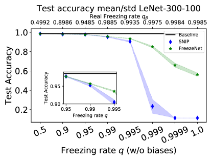
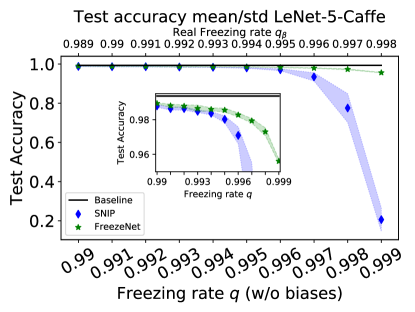
Figure 2: Left: Test accuracy for SNIP, FreezeNet and the baseline LeNet-$300$-$100$. Right: Test accuracy for SNIP and FreezeNet for a LeNet-5-Caffe baseline. The small inserted plots are zoomed in versions for both plots.

4.1.1 LeNet-$300$-$100$

A common baseline to examine pruning mechanisms on fully connected networks is given by testing the LeNet-$300$-$100$ [27] network on the MNIST classification task [27], left part of Figure 2. The trained baseline architecture yields a mean test accuracy of $98.57\%$. If the freezing rate is lower than $0.95$, both methods perform equally well and also match the performance of the baseline. For higher freezing rates, the advantage of using free, additional parameters can be seen. FreezeNets also suffer from the loss of trainable weights, but they are able to compensate it better than SNIP pruned networks do.

Table 2: Comparison of FreezeNet, SNIP and the LeNet-$5$-Caffe baseline. Results for different freezing rates $q$ with corresponding real freezing rates $q_{\beta}$ are displayed. The network’s size is calculated without compression. Thus, all weights are stored as $32$bit floats. Compress. Factor FN is the compression factor gained by FreezeNet for the corresponding freezing rate, calculated via the ratio of the network sizes of the baseline and the frozen network.

$q$	$q_{\beta}$	Network Size	Compress. Factor FN	Test Acc. SNIP	Test Acc. FreezeNet	$\frac{\text{FreezeNet Acc.}}{\text{Baseline Acc.}}$
$0$ (Baseline)		$1,683.9$kB	$1$	$99.36\%$		$1.000$
$0.9$	$0.899$	$170.7$kB	$\bm{9.9}$	$99.24\%$	$\bm{99.37\%}$	$1.000$
$0.99$	$0.989$	$19.1$kB	$\bm{88.2}$	$98.80\%$	$\bm{98.94\%}$	$0.996$
$0.995$	$0.994$	$10.7$kB	$\bm{157.4}$	$98.02\%$	$\bm{98.55\%}$	$0.992$
$0.999$	$0.998$	$3.9$kB	$\bm{431.8}$	$20.57\%$	$\bm{95.61\%}$	$0.962$

4.1.2 LeNet-$5$-Caffe

For moderate freezing rates $q\in[0.5,0.95]$, again FreezeNet and SNIP reach equal results and match the baseline’s performance as shown in the Supplementary Material. In the right part of Figure 2, we show the progression of SNIP and FreezeNet for more extreme freezing rates $q\in\{0.99,0.991,\ldots,0.999\}$. Until $q=0.994$ SNIP and FreezeNet perform almost equally, however FreezeNet reaches slightly better results. For higher freezing rates, SNIP’s performance drops steeply whereas FreezeNet is able to slow this drop. As Table 2 and Figure 2 show, a FreezeNet saves parameters with respect to both, the baseline architecture and a SNIP pruned network.

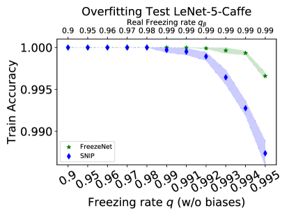
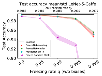
Figure 3: Left: Final training accuracies for FreezeNet and SNIP, both trained without weight decay. Right: Different initializations for FreezeNets together with a Xavier-normal initialized FreezeNet with randomly generated freezing mask. Both plots are reported for the MNIST classification task with a LeNet-$5$-Caffe baseline architecture.

In order to overfit the training data maximally, we change the training setup by training the networks without the usage of weight decay and early stopping. In the left part of Figure 3, the training accuracies of FreezeNet and SNIP are reported for the last training epoch. Unsurprisingly, too many frozen parameters reduce the model’s capacity, as the model is not able to perfectly memorize the training data for rates higher than $q_{\ast}=0.992$. On the other hand, FreezeNets increase the networks capacity compared to SNIP if the same, high freezing rate is used.

4.2 Testing FreezeNets for CIFAR-$10$/$100$ on VGG$16$-D

Table 3: Comparison of results for the CIFAR-$10$/$100$ tasks with a VGG$16$-D baseline.

			CIFAR-$\bm{10}$	CIFAR-$\bm{100}$
Method	Freezing Rate	Trained Parameters	Mean $\pm$ Std	Mean $\pm$ Std
Baseline	$0$	$15.3$mio	$\bm{93.0\pm 0.1\%}$	$\bm{71.6\pm 0.6}\%$
SNIP	$0.9$	$1.5$mio	$92.9\pm 0.1\%$	$53.9\pm 1.7\%$
	$0.95$	$780$k	$92.5\pm 0.1\%$	$48.6\pm 6.6\%$
	$0.99$	$169$k	$10.0\pm 0.0\%$	$1.0\pm 0.0\%$
	$0.995$	$92$k	$10.0\pm 0.0\%$	$1.0\pm 0.0\%$
FreezeNet	$0.9$	$1.5$mio	$92.2\pm 0.1\%$	$\bm{70.7\pm 0.3}\%$
	$0.95$	$780$k	$91.7\pm 0.1\%$	$\bm{69.0\pm 0.2}\%$
	$0.99$	$169$k	$\bm{88.6\pm 0.1\%}$	$\bm{59.8\pm 0.3}\%$
	$0.995$	$92$k	$\bm{86.0\pm 0.1\%}$	$\bm{53.4\pm 0.1}\%$
FreezeNet-WD	$0.9$	$1.5$mio	$\bm{93.2\pm 0.2\%}$	$53.1\pm 1.8\%$
	$0.95$	$780$k	$\bm{92.8\pm 0.2\%}$	$44.5\pm 5.4\%$
	$0.99$	$169$k	$76.1\pm 1.0\%$	$13.1\pm 1.8\%$
	$0.995$	$92$k	$74.6\pm 1.1\%$	$11.9\pm 1.4\%$

To test FreezeNets on bigger architectures, we use the VGG$16$-D architecture [37] and the CIFAR-$10$/$100$ datasets. Now, weight decay is applied to all parameters, including the frozen ones, denoted with FreezeNet-WD. As before, weight decay is also used on the unfrozen parameters only, which we again call FreezeNet. We follow the settings in [29] and exchange Dropout layers with Batch Normalization [23] layers. Including the Batch Normalization parameters, the VGG$16$-D network consists of $15.3$ million parameters in total. We train all Batch Normalization parameters and omit them in the freezing rate $q$. Additionally, we augment the training data by random horizontal flipping and translations up to $4$ pixels. For CIFAR-$100$ we report results for networks initialized with a Kaiming-uniform initialization [21]. The results are summarized in Table 3.

4.2.1 CIFAR-$10$

If more parameters are trainable, $q\leq 0.95$, SNIP performs slightly worse than the baseline but better than FreezeNet. However, using frozen weights can achieve similar results as the baseline architecture while outperforming SNIP if weight decay is applied to them as well, as shown with FreezeNet-WD. Applying weight decay also on the frozen parameters solely shrinks them to zero. For all occasions where FreezeNet-WD reaches the best results, the frozen weights can safely be pruned at the early stopping time, as they are all shrunk to zero at this point in training. For these freezing rates, FreezeNet-WD can be considered as a pruning mechanism outperforming SNIP without adding any gradient computations For higher freezing rates $q\geq 0.99$, FreezeNet still reaches reasonable results whereas FreezeNet-WD massively drops performance and SNIP even results in random guessing.

4.2.2 CIFAR-$100$

CIFAR-$100$ is more complex to solve than CIFAR-$10$. As the right part of Table 3 shows, SNIP is outperformed by FreezeNet for all freezing rates. Frozen parameters seem to be even more helpful for a sophisticated task. For CIFAR-$100$, more complex information flows backwards during training, compared to CIFAR-$10$. Thus, using dense weight matrices in the backward pass helps to provide enough information for the gradients to train successfully. Additionally we hypothesize, that random features generated by frozen parameters can help to improve the network’s performance, as more and often closely related classes have to be distinguished. Using small, randomly generated differences between data samples of different, but consimilar classes may help to separate them.

4.2.3 Discussion

Deleting the frozen weights reduces the network’s capacity — as shown for the MNIST task, Figure 3 left. But for small freezing rates, the pruned network still has enough capacity in the forward- and backward propagation. In these cases, the pruned network has a higher generalization capability than the FreezeNet, according to the bias-variance trade-off [15]. Continuously decreasing the network’s capacity during training, instead of one-shot, seems to improve the generalization capacity even more, as done with FreezeNet-WD. But for higher freezing rates, unshrunken and frozen parameters improve the performance significantly. For these rates, FreezeNet is still able to learn throughout the whole training process. Whereas FreezeNet-WD reaches a point in training, where the frozen weights are almost zero. Therefore, the gradient does not flow properly through the network, since the pruned SNIP network has zero gradient flow for these rates, Figure 4 left. This change of FreezeNet-WD’s gradient’s behaviour is shown in Figure 4 right for $q=0.99$. It should be mentioned that in these cases, FreezeNet-WD will have an early stopping time before all frozen weights are shrunk to zero and FreezeNet-WD can not be pruned without loss in performance.

4.3 Gradient Flow

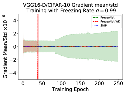
Figure 4: Left: Shows the relative gradient norm for FreezeNet, SNIP and GraSP networks with respect to the VGG$16$-D baseline network on the CIFAR-$10$ dataset. Right: Gradient mean and std, computed over the training data, recorded for one training run with a VGG$16$-D architecture on the CIFAR-$10$ task for a freezing rate $q=0.99$.

As theoretically discussed in Section 3.2, FreezeNets help to preserve a strong gradient, even for high freezing rates. To check this, we also pruned networks with the GraSP criterion [39] to compare FreezeNets with pruned networks generated to preserve the gradient flow. A detailed description of the GraSP criterion can be found in the Supplementary Material. For this test, $10$ different networks were initialized for every freezing rate and three copies of each network were frozen (FreezeNet) or pruned (SNIP and GraSP), respectively. The $L_{1}$ norm of the gradient, accumulated over the whole training set, is divided by the number of trainable parameters. As reference, the mean norm of the baseline VGG$16$-D’s gradient is measured as well. These gradient norms, computed for CIFAR-$10$, are compared in the left part of Figure 4. For smaller freezing rates, all three methods have bigger gradient values than the baseline, on average. For rates $q\geq 0.95$, decreasing the number of trainable parameters leads to a reduced gradient flow for the pruned networks. Even if the pruning mask is chosen to guarantee the highest possible gradient flow, as approximately done by GraSP. Finally, the gradient vanishes, since the weight tensors become sparse for high pruning rates, as already discussed in Section 3.2. FreezeNet’s gradient on the other hand is not hindered since its weight tensors are dense. The saliency score (1) is biased towards choosing weights with a high partial derivative. Therefore, FreezeNet’s non-zero gradient values even become larger as the number of trainable parameters decreases. For high freezing rates, FreezeNet’s gradient is able to flow through the network during the whole training process, whereas SNIP’s gradient remains zero all the time — right part of Figure 4. The right part of Figure 4 also shows the mutation of FreezeNet-WD’s gradient flow during training. First, FreezeNet-WD has similar gradients as FreezeNet since the frozen weights are still big enough. The red peak indicates the point where too many frozen weights are shrunken close to zero, leading to temporarily chaotic gradients and resulting in zero gradient flow.

4.4 Comparison to Pruning Methods

Especially for extreme freezing rates, we see that FreezeNets perform remarkably better than SNIP, which often degenerates to random guessing. In Table 4, we compare our result for LeNet-$5$-Caffe with Sparse-Momentum [7], SNIP, GraSP and three other pruning methods Connection-Learning [19], Dynamic-Network-Surgery [17] and Learning-Compression [3]. Up to now, all results are reported without any change in hyperparameters. To compare FreezeNet with other pruning methods, we change the training setup slightly by using a split of $19/1$ for train and validation images for FreezeNet, but keep the remaining hyperparameters fixed. We also recreated results for GraSP [39]. The training setup and the probed hyperparameters for GraSP can be found in the Supplementary Material. All other results are reported from the corresponding papers. As shown in Table 4, the highest accuracy of $99.2\%$ is achieved by the methods Connection-Learning and Sparse-Momentum. With an accuracy of $99.1\%$ our FreezeNet algorithm performs only slightly worse, however Connection-Learning trains $8.3\%$ of its weights — whereas FreezeNet achieves $99.37\%$ accuracy with $10\%$ trained weights, see Table 2. Sparse-Momentum trains with sparse weights, but updates the gradients of all weights during training and redistributes the learnable weights after each epoch. Thus, their training procedure does neither provide sparse gradient computations nor one-shot pruning and is hence more expensive than FreezeNet. Apart from that, FreezeNet achieves similar results to Dynamic-Network-Surgery and better results than Learning-Compression, GraSP and SNIP, while not adding any training costs over GraSP and SNIP and even reducing them for Dynamic-Network-Surgery and Learning-Compression.

Table 4: Comparison of different pruning methods with FreezeNet on LeNet-5-Caffe.

Method	Sparse Gradients in Training	Additional Hyperparameters	Percent of trainable parameters	Test Accuracy
Baseline [27]	$-$	$-$	$100\%$	$99.4\%$
SNIP [29]	✓	✗	$1.0\%$	$98.9\%$
GraSP [39]	✓	✗	$1.0\%$	$98.9\%$
Connection-Learning [19]	✗	✗	$8.3\%$	$99.2\%$
Dynamic-Network-Surgery [17]	✗	✗	$0.9\%$	$99.1\%$
Learning-Compression [3]	✗	✓	$1.0\%$	$98.9\%$
Sparse-Momentum [7]	✗	✓	$1.0\%$	$99.2\%$
FreezeNet (ours)	✓	✗	$1.0\%$	$99.1\%$

4.5 Further Investigations

The right part of Figure 3 shows on the one hand, that FreezeNet reaches better and more stable results than freezing networks with a randomly generated freezing mask. This accentuates the importance of choosing the freezing mask consciously, for FreezeNets done with the saliency score (1).

On the other hand, different variance scaling initialization schemes are compared for FreezeNets in the right part of Figure 3. Those initializations help to obtain a satisfying gradient flow at the beginning of the training [16, 21]. Results for the Xavier-normal initialization [16], the Kaiming-uniform [21] and the ${\tt pm}_{\sigma}$-initialization are shown. All of these initializations lead to approximately the same results. Considering all freezing rates, the Xavier-initialization yields the best results. The ${\tt pm}_{\sigma}$-initialization is a variance scaling initialization, using zero mean and a variance of ${\sigma^{2}=\frac{2}{fan_{in}+fan_{out}}}$, layerwise. All weights are set to $+\sigma$ with probability $\frac{1}{2}$ and $-\sigma$ otherwise. Using the ${\tt pm}_{\sigma}$-initialization shows, that even the simplest variance scaling method leads to good results for FreezeNets.

In the Supplementary Material we exhibit that FreezeNets are robust against reinitializations of their weights after the freezing mask is computed and before the actual training starts. The probability distribution can even be changed between initialization and reinitialization while still leading to the same performance.

5 Conclusions

With FreezeNet we have introduced a pruning related mechanism that is able to reduce the number of trained parameters in a neural network significantly while preserving a high performance. FreezeNets match state-of-the-art pruning algorithms without using their sophisticated and costly training methods, as Table 4 demonstrates. We showed that frozen parameters help to overcome the vanishing gradient occurring in the training of sparse neural networks by preserving a strong gradient signal. They also enhance the expressiveness of a network with few trainable parameters, especially for more complex tasks. With the help of frozen weights, the number of trained parameters can be reduced compared to the related pruning method SNIP. This saves storage space and thus reduces transfer costs for trained networks. For smaller freezing rates, it might be better to weaken the frozen parameters’ influence, for example by applying weight decay to them. Advantageously, using weight decay on frozen weights contracts them to zero, leading to sparse neural networks. But for high freezing rates, weight decay in its basic form might not be the best regularization mechanism to apply to FreezeNets, since only shrinking the frozen parameters robs them of a big part of their expressiveness in the forward and backward pass.

S1 Supplementary Material for FreezeNet: Full Performance by Reduced Storage Costs

S1.1 Training Hyperparameters for MNIST and CIFAR-$10$

Our results in the main body of the text are benchmarked against SNIP [29], since we share its feature selection and it is also a one-shot method, applied before training. For the comparison we use their training schedule and do not tune any hyperparameters. They take a batch size of $100$ (MNIST) or $128$ (CIFAR) and SGD with momentum parameter $0.9$ [38] as optimizer. The initial learning rate is set to $0.1$ and divided by ten at every $25$k/$30$k optimization steps for MNIST and CIFAR, respectively. For regularization, weight decay with coefficient $5\cdot 10^{-4}$ is applied. The overall number of training epochs is $250$.

S1.2 Tiny ImageNet Experiment

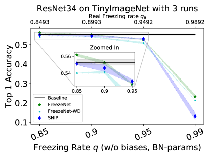
Figure S1: Comparison of FreezeNet, FreezeNet-WD and SNIP for a ResNet$34$ trained on Tiny ImageNet.

In addition to the MNIST and CIFAR experiments, we also tested FreezeNet on a ResNet$34$ [21] on the Tiny ImageNet classification task . The ResNet$34$ architecture is shown in Table S5. The Tiny ImageNet dataset consists of $64\times 64$ RGB images with $200$ different classes. Those classes have $500$ training images, $50$ validation images and $50$ test images, each. For training, we use the same data augmentation as for CIFAR, i.e. random horizontal flipping and translations up to $4$ pixels. We train the network for $100$ epochs with an initial learning rate of $0.01$. The learning rate is decayed by a factor $10$ after epoch $30$, $60$ and $80$. As optimizer, again SGD with momentum parameter $0.9$ is used. Also, weight decay with coefficient $5\cdot 10^{-4}$ is applied. The networks are initialized with a Kaiming-uniform initialization.

In Figure S1, the results for FreezeNet, FreezeNet-WD and SNIP are shown. The mean and standard deviation for every freezing rate and method are each calculated for three runs with different random seeds. We see, that FreezeNet can be used to train a ResNets successfully. FreezeNet has the same accuracy than the baseline method while training only $10\%$ of its weights. For all rates, FreezeNet achieves better or equal results than SNIP. Also, FreezeNet’s results are more stable, shown by the slimmer standard deviation bands. Contrarily to the CIFAR-$10$ experiment, FreezeNet-WD shows worse results than SNIP for lower freezing rates. Reaching good results with a FreezeNet on ResNet$34$ needs a higher rate of trainable parameters than on VGG$16$, see Table 3.

S1.3 GraSP

The GraSP criterion [39] is based on the idea of preserving, or even increasing, the pruned network’s gradient flow compared to the unpruned counterpart. Thus,

$$\Delta L(W):=\left\|\frac{\partial L}{\partial W}\right\|_{2}^{2}$$ (S.1)

is tried to be maximized with the masked weights $m\odot W$. For that purpose,

$$\Delta L(m\odot W)\approx\Delta L(W)-W^{T}\cdot H_{L}\cdot\frac{\partial L}{\partial W}+\left(m\odot W\right)^{T}\cdot H_{L}\cdot\frac{\partial L}{\partial W}$$ (S.2)

is approximated via the first order Taylor series, with the Hessian $H_{L}:=\frac{\partial^{2}L}{\partial W^{2}}\in\mathbb{R}^{D\times D}$. As $\Delta L(W)-W^{T}\cdot H_{L}\cdot\frac{\partial L}{\partial W}$ is fix, the importance score for all weights $W\in\mathbb{R}^{D}$ is computed as

$$S(W):=W\odot\left(H_{L}\cdot\frac{\partial L}{\partial W}\right)$$ (S.3)

and the weights with the $1-q$ highest importance scores are trained, the other ones are pruned. Contrarily to the saliency score (1), the importance score (S.3) takes the sign into account. Pruning with the GraSP criterion is applied, as SNIP and FreezeNet, once before the training starts [39]. Thus, GraSP pruned networks also have sparse gradients during training.

S1.3.1 Training Setup for Result in Table 4

Different freezing rates are displayed in Table 4, as we first tried to find results in the corresponding papers with freezing rates approximately $q=0.99$. If no result for such a freezing rate was given, we report the result with the closest accuracy to FreezeNet’s performance for $q=0.99$.

We used the experimental setup described in Section 4 with hyperparameters from Section S1.1. The official method to calculate the GraSP score was used. Moreover, learning rates $2^{n}\cdot 0.1$ with $n\in\{-4,\ldots,4\}$ were tested for a split of training/validation images of $9/1$, $19/1$ and $3/1$. Each of these $27$ combinations was run $5$ times with a different initialization. For each combination, the network with the best validation accuracy was tested at its early stopping time. The best result was reported for the learning rate $\lambda=0.1$ with a split of training/validation images of $19$/$1$ — the same setup as used for the best FreezeNet result. The reported test accuracy for the GraSP pruned network is given by $98.9\%$.

S1.4 Reinitialization Tests

Up to now it is unanswered how the reinitialization of a network’s weights after the calculation of the saliency scores affects the trainability of this network. To check this, we modify Algorithm 1 by adding a reinitialization step after the computation of the saliency score. FreezeNets with reinitializations are introduced in Algorithm S1.

1:Freezing rate $q$, initial parametrization $\Theta_{0}=W_{0}\cup B_{0}$, reinitialized parameters $\Theta_{1}=W_{1}\cup B_{1}$, network $f$, loss function $L$

2:

3:Calculate saliency score $g\in\mathbb{R}^{|W_{0}|}$ according to equation (1) with $f_{\Theta_{0}}$ for one training batch

4:Define freezing mask $m\in\mathbb{R}^{|W_{0}|}$

5:Calculate freezing threshold $\varepsilon$, where $\varepsilon$ denotes the $\lfloor(1-q)\cdot|W_{0}|\rfloor$-highest magnitude of $g$

6:Set $m_{k}=0$ if $|g_{k}|<\varepsilon$ else $m_{k}=1$

7:Set networks parameters to $\Theta_{1}$, i.e. use $f_{\Theta_{1}}$ for training

8:Start training with forward propagation as usual but backpropagate gradient ${m\odot\frac{\partial L}{\partial W_{1}}}$ for weights and $\frac{\partial L}{\partial B_{1}}$ for biases

Algorithm S1 FreezeNet with Reinitialization after Computation of Freezing Mask

We have tested a LeNet-$5$-Caffe baseline architecture for MNIST on Algorithm S1. Again we follow the training setup from Sections 4 together with S1.1.

First we tested combinations of initializing and reinitializing a FreezeNet with the Xavier-normal and the Kaiming-uniform initialization schemes. We name the network without reinitialized weights FreezeNet-K for a Kaiming-uniform initialized network, or FreezeNet-X for a Xavier-normal initialized one. The reinitialized networks are denoted as FreezeNet-A-B for $\text{A,B}\in\{\text{K,X}\}$ where A stands for the initialization used for finding the freezing mask and B for the reinitialization, applied before training.

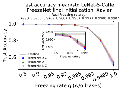
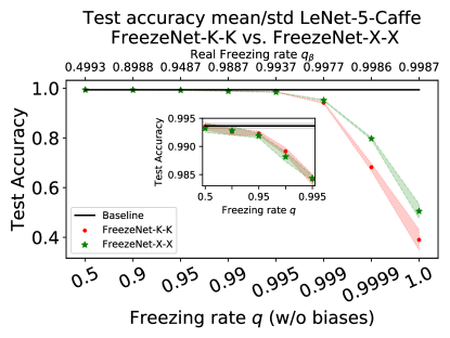
Figure S2: LeNet-$5$-Caffe baseline architecture compared to a FreezeNet-X, a FreezeNet-X-X and a FreezeNet-K-X in the left plot. On the right side we compare a FreezeNet-X-X with a FreezeNet-K-K. Inserted: Zoomed in versions of the plots.

The left plot in Figure S2 compares FreezeNet-X with FreezeNet-X-X and FreezeNet-K-X. This graph shows, that reinitializations do not significantly change the performance of FreezeNets. It also does not seem to make a difference if the probability distribution used for the reinitialization differs from the one used to calculate the freezing mask, examined through FreezeNet-K-X and FreezeNet-X-X. Similar results are reported for the comparison of FreezeNet-K with FreezeNet-K-K and FreezeNet-X-K, shown in the left part of Figure S3.

In Figure S3, right plot, various other reinitialization methods are tested on a Xavier-normal initialized FreezeNet. We can see, that the variance scaling reinitialization methods Xavier-normal, Kaiming-uniform and ${\tt pm}_{\sigma}$ lead to the same results. The ${\tt pm}_{\sigma}$ initialization scheme is introduced in Section 4.5 in the main body of the text. Using other, non-variance scaling methods as constant reinitialization (either with all values $1$ or the layers variance $\sigma$) or drawing weights i.i.d. from $\mathcal{N}(0,1)$ generates networks which cannot be trained at all.

The right plot in Figure S2 shows that the initialization, used after the freezing mask is computed, is important to solve the MNIST task successfully for high freezing rates. The Kaiming init- and reinitialization, FreezeNet-K-K, performs slightly better for the lower freezing rates and is outperformed by FreezeNet-X-X for the higher ones. Without reinitialization, a similar behaviour for low and high freezing rates can be seen in Figure 3 — right plot.

Summarized, using an appropriate initialization scheme for the weights, after the freezing mask is computed, is essential for achieving good results with FreezeNets. Based on our experiments we suggest initializing (and reinitializing, if wanted) FreezeNets with variance scaling methods.

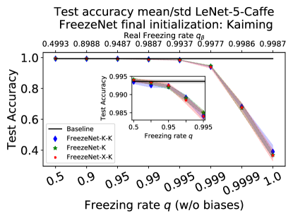
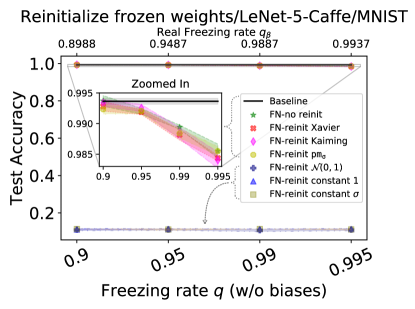
Figure S3: Left: LeNet-$5$-Caffe baseline architecture with a corresponding FreezeNet-K, a FreezeNet-K-K and a FreezeNet-X-K. Right: Comparison of different reinitializations for a FreezeNet (FN) with LeNet-$5$-Caffe baseline architecture with Xavier-normal initialization. Inserted: Zoomed in versions of the plots.

S1.5 Learning Rate Experiments

SGD is used in our experiments, thus we also tested a broad range of learning rates for different freezing rates. This test was done with the same setup as described in Sections 4 and S1.1. The results for a LeNet-$5$-Caffe baseline architecture on the MNIST classification task are shown in Figures S4 and S5. In order to cover a broad range of learning rates, we used $2^{n}\cdot\lambda_{0},n\in\{-4,-3,\ldots,4\}$ and $\lambda_{0}=0.1$ as learning rates. All learning and freezing rate combinations were trained with three different random initializations. The learning rates with the best results are shown in the left part of Figure S4. For almost any freezing rate, the learning rate $0.1$ works best. Thus, FreezeNets do not need expensive learning rate searches but can use a learning rate performing well on the baseline architecture. But optimizing the learning rate can improve FreeNets’ performance beyond question. Another conclusion we want to highlight is that higher learning rates can be applied for higher freezing rates. Even if they do not work well for smaller freezing rates, as the example of $\lambda=0.2$ in the left part of Figure S4 shows. The same holds for learning rates bigger than $0.2$, which require even higher freezing rates to lead to satisfying results, as shown in the right part of Figure S5. For high freezing rates, using higher learning rates can lead to better and faster training, as shown in Figure S4, right side.

The results for the learning rate search for the CIFAR$10$ task with a VGG$16$-D are shown in Figure S6. Again, $\lambda_{0}=0.1$ performs best for most of the freezing rates and is only slightly improved for some freezing rates by $\lambda=0.2$ and $\lambda=0.05$.

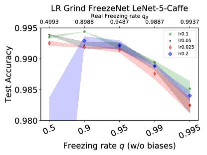
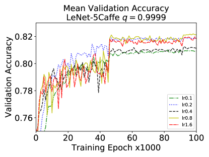
Figure S4: Learning rate tests for a FreezeNet with a LeNet-$5$-Caffe baseline. The left part shows the mean test accuracy for the best performing learning rates. The right plot shows the mean validation accuracy for three training runs recorded over the first $100$k epochs for different learning rates.

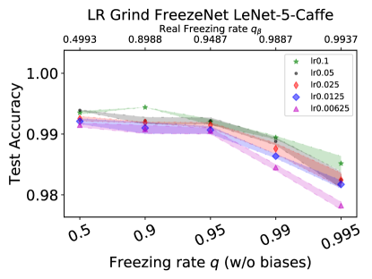
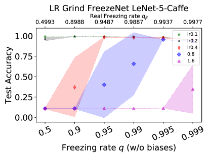
Figure S5: Learning rate tests for a FreezeNet with a LeNet-$5$-Caffe baseline. The left part shows the mean test accuracy for the learning rates $\lambda\leq\text{0.1}$. The right plot shows the mean validation accuracy for the learning rates $\lambda\geq 0.1$.

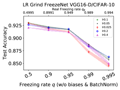
Figure S6: Best performing learning rates for a FreezeNet with a VGG$16$-D baseline on the CIFAR-$10$ classification task.

S1.6 Figures for LeNet-$5$-Caffe on MNIST

Figure S7 shows the comparison of FreezeNet and SNIP over a broad range of freezing rates, discussed in Section 4.1. Here, the networks are trained and evaluated as described in Section 4 with hyperparameters from Section S1.1.

The training progress of FreezeNet’s result, reported in Table 4, is shown in Figure S8.

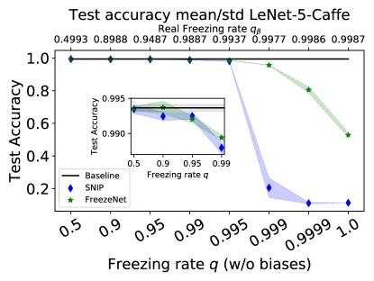
Figure S7: Comparison SNIP and FreezeNet for the MNIST classification task and a LeNet-$5$-Caffe baseline architecture. The inserted plot is a zoomed version.

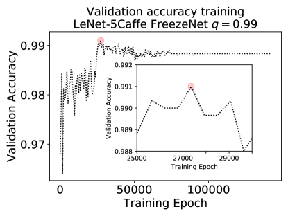
Figure S8: Training of FreezeNet for freezing rate $q=0.99$ and baseline architecture LeNet-$5$-Caffe. Training procedure is done as described in Section S1.1 with hyperparameters from Section S1.1 but with a split $19/1$ of training and validation images. This plot shows the run with the best validation accuracy out of five tries. The corresponding test accuracy equals $99.1\%$, calculated with the weights stored in the early stop epoch, as reported in Table 4. The red circle highlights the epoch where early stopping occurs. The inserted plot is a zoomed version showing the early stopping epoch.

S1.7 Network Architectures

Figures S9, S10 and S11 visualize the used LeNet-$300$-$100$, LeNet-$5$-Caffe and VGG$16$-D network architectures, respectively. The ResNet$34$ architecture can be looked up in Table S5 together with Figure S12.

Figure S9: Architecture of the used LeNet-$300$-$100$. In front of the first layer, the feature map $x\in\mathbb{R}^{1\times 28\times 28}$ is flattened to $\hat{x}\in\mathbb{R}^{784}$. For linear layers, $n_{in}$ and $n_{out}$ denote the number of incoming and outgoing neurons, respectively.

Figure S10: Architecture of the used LeNet-$5$-Caffe. All 2D-convolutional layers have kernel size $5\times 5$, $1\times 1$ stride and no zero padding. A max-pooling layer has kernel size $2\times 2$, stride $2\times 2$ and dilation $1\times 1$. Before entering the first linear layer, the feature map $\hat{x}\in\mathbb{R}^{50\times 4\times 4}$ is flattened to $\hat{\hat{x}}\in\mathbb{R}^{800}$. The resolutions left to the blocks denote the resolution of the feature maps, processed by the corresponding layers. For convolutional layers, $n_{in}$ and $n_{out}$ denote the number of incoming and outgoing channels, respectively. For linear layers, $n_{in}$ and $n_{out}$ denote the number of incoming and outgoing neurons, respectively.

Figure S11: Architecture of VGG$16$-D. Here, $n_{c}\in\{10,100\}$ equals the numbers of classes for the given classification task. For CIFAR-$10$, $n_{c}=10$ and for CIFAR-$100$ we have $n_{c}=100.$ A ConvBlock consists of a 2D-convolutional layer with kernel size $3\times 3$, and $1\times 1$ stride and padding. Each convolution is followed by a $2$D-Batch Normalization Layer and a ReLU activation function. The max-pooling layer has kernel size $2\times 2$, stride $2\times 2$ and dilation $1\times 1$. Before entering the first LinearBlock, the feature map $\hat{x}\in\mathbb{R}^{512\times 1\times 1}$ is flattened to $\hat{\hat{x}}\in\mathbb{R}^{512}$. A LinearBlock consist of a fully connected layer followed by a $1$D-Batch Normalization Layer and a ReLU activation function. The resolution left to the blocks denotes the resolution of the feature maps, processed by the corresponding blocks. For Convolutional blocks, $n_{in}$ and $n_{out}$ denote the number of incoming and outgoing channels, respectively. For linear blocks and layers, $n_{in}$ and $n_{out}$ denote the number of incoming and outgoing neurons, respectively.

Table S5: ResNet$34$ with ResBlocks, shown in Figure S12. The kernel size is given by $k$. For Convolutional layers and ResBlocks, $n_{in}$ and $n_{out}$ denote the number of incoming and outgoing channels, respectively. For the linear layer, $n_{in}$ and $n_{out}$ denote the number of incoming and outgoing neurons, respectively. Before entering the linear layer, the feature map $x\in\mathbb{R}^{512\times 1\times 1}$ is flattened to $\hat{x}\in\mathbb{R}^{512}$. A ResNet$34$ consists of $21,383,816$ parameters in total. Thereof, $21,366,464$ weights, $200$ biases and $17,152$ BatchNorm parameters.

Module	Output Size	Repeat	$n_{in}$	$n_{out}$	$k$	Stride	Padding	Bias	BatchNorm	ReLU
Conv2D	$64\times 64$	$\times 1$	$3$	$64$	$3$	$1$	$1$	✗	✓	✓
ResBlock	$32\times 32$	$\times 1$	$64$	$64$	$3$	$2$	$1$	✗	✓	✓
ResBlock	$32\times 32$	$\times 2$	$64$	$64$	$3$	$1$	$1$	✗	✓	✓
ResBlock	$16\times 16$	$\times 1$	$64$	$128$	$3$	$2$	$1$	✗	✓	✓
ResBlock	$16\times 16$	$\times 3$	$128$	$128$	$3$	$1$	$1$	✗	✓	✓
ResBlock	$8\times 8$	$\times 1$	$128$	$256$	$3$	$2$	$1$	✗	✓	✓
ResBlock	$8\times 8$	$\times 5$	$256$	$256$	$3$	$1$	$1$	✗	✓	✓
ResBlock	$4\times 4$	$\times 1$	$256$	$512$	$3$	$2$	$1$	✗	✓	✓
ResBlock	$4\times 4$	$\times 2$	$512$	$512$	$3$	$1$	$1$	✗	✓	✓
AvgPool2D	$1\times 1$	$\times 1$	$512$	$512$	$4$	$0$	$0$	✗	✗	✗
Linear	$200$	$\times 1$	$512$	$200$	—	—	—	✓	✗	✗
log softmax	$10$	$\times 1$	$200$	$200$	—	—	—	✗	✗	✗

Figure S12: Architecture of a ResBlock with $n_{in}$ input channels, $n_{out}$ output channels and stride $s$ for the first convolution. The second $3\times 3$ conolution has stride $1$ and $n_{out}$ in- and output channels. Shortcut connections are a $1\times 1$ 2D Convolution with $n_{in}$ input and $n_{out}$ output channels and stride $s$ followed by a BatchNorm2D layer if $n_{in}\neq n_{out}$. Otherwise, Shortcut connections are simply given by the Identity function. All Conv2D layers are initialized without biases.

References

- [1] Abadi, M., Agarwal, A., Barham, P., Brevdo, E., Chen, Z., Citro, C., et al.: Tensorflow: Large-scale machine learning on heterogeneous distributed systems. CoRR abs/1603.04467 (2016)
- [2] Bellec, G., Kappel, D., Maass, W., Legenstein, R.: Deep rewiring: Training very sparse deep networks. In: International Conference on Learning Representations. OpenReview.net (2018)
- [3] Carreira-Perpinan, M.A., Idelbayev, Y.: ”Learning-compression” algorithms for neural net pruning. In: 2018 IEEE/CVF Conference on Computer Vision and Pattern Recognition. pp. 8532–8541. IEEE Computer Society (2018)
- [4] Chauvin, Y.: A back-propagation algorithm with optimal use of hidden units. In: Touretzky, D.S. (ed.) Advances in Neural Information Processing Systems 1. Morgan-Kaufmann (1989)
- [5] Davis, C.: The norm of the schur product operation. Numerische Mathematik 4(1), 343–344 (1962)
- [6] Deng, J., Dong, W., Socher, R., Li, L., Li, K., Fei-Fei, L.: Imagenet: A large-scale hierarchical image database. In: 2009 IEEE Conference on Computer Vision and Pattern Recognition. pp. 248–255. IEEE Computer Society (2009)
- [7] Dettmers, T., Zettlemoyer, L.: Sparse networks from scratch: Faster training without losing performance. CoRR abs/1907.04840 (2019)
- [8] Ding, X., Ding, G., Zhou, X., Guo, Y., Han, J., Liu, J.: Global sparse momentum sgd for pruning very deep neural networks. In: Wallach, H., Larochelle, H., Beygelzimer, A., d’ Alché-Buc, F., Fox, E., Garnett, R. (eds.) Advances in Neural Information Processing Systems 32, pp. 6382–6394. Curran Associates, Inc. (2019)
- [9] Dong, X., Huang, J., Yang, Y., Yan, S.: More is less: A more complicated network with less inference complexity. 2017 IEEE Conference on Computer Vision and Pattern Recognition (CVPR) (2017)
- [10] Dong, X., Yang, Y.: Network pruning via transformable architecture search. In: Wallach, H., Larochelle, H., Beygelzimer, A., d’ Alché-Buc, F., Fox, E., Garnett, R. (eds.) Advances in Neural Information Processing Systems 32, pp. 760–771. Curran Associates, Inc. (2019)
- [11] Duda, J., Tahboub, K., Gadgil, N.J., Delp, E.J.: The use of asymmetric numeral systems as an accurate replacement for huffman coding. In: Picture Coding Symposium. pp. 65–69 (2015)
- [12] Frankle, J., Carbin, M.: The lottery ticket hypothesis: Finding sparse, trainable neural networks. In: International Conference on Learning Representations (2018)
- [13] Frankle, J., Dziugaite, G.K., Roy, D.M., Carbin, M.: Stabilizing the lottery ticket hypothesis. CoRR abs/1903.01611 (2019)
- [14] Frankle, J., Schwab, D.J., Morcos, A.S.: Training batchnorm and only batchnorm: On the expressive power of random features in cnns. CoRR abs/2003.00152 (2020)
- [15] Geman, S., Bienenstock, E., Doursat, R.: Neural networks and the bias/variance dilemma. Neural Comput. 4(1), 1–58 (1992)
- [16] Glorot, X., Bengio, Y.: Understanding the difficulty of training deep feedforward neural networks. In: Teh, Y.W., Titterington, M. (eds.) Proceedings of the Thirteenth International Conference on Artificial Intelligence and Statistics. pp. 249–256. PMLR (2010)
- [17] Guo, Y., Yao, A., Chen, Y.: Dynamic network surgery for efficient dnns. In: Lee, D.D., Sugiyama, M., Luxburg, U.V., Guyon, I., Garnett, R. (eds.) Advances in Neural Information Processing Systems 29, pp. 1379–1387. Curran Associates, Inc. (2016)
- [18] Gustafson, J.L.: Moore’s law. In: Padua, D. (ed.) Encyclopedia of Parallel Computing. pp. 1177–1184. Springer US (2011)
- [19] Han, S., Pool, J., Tran, J., Dally, W.: Learning both weights and connections for efficient neural network. In: Cortes, C., Lawrence, N.D., Lee, D.D., Sugiyama, M., Garnett, R. (eds.) Advances in Neural Information Processing Systems 28. Curran Associates, Inc. (2015)
- [20] Hanson, S.J., Pratt, L.Y.: Comparing biases for minimal network construction with back-propagation. In: Touretzky, D.S. (ed.) Advances in Neural Information Processing Systems 1. Morgan-Kaufmann (1989)
- [21] He, K., Zhang, X., Ren, S., Sun, J.: Delving deep into rectifiers: Surpassing human-level performance on imagenet classification. CoRR abs/1502.01852 (2015)
- [22] He, Y., Lin, J., Liu, Z., Wang, H., Li, L.J., Han, S.: Amc: Automl for model compression and acceleration on mobile devices. Lecture Notes in Computer Science p. 815–832 (2018)
- [23] Ioffe, S., Szegedy, C.: Batch normalization: Accelerating deep network training by reducing internal covariate shift. In: Bach, F., Blei, D. (eds.) Proceedings of the 32nd International Conference on Machine Learning. pp. 448–456. PMLR (2015)
- [24] Jarrett, K., Kavukcuoglu, K., Ranzato, M., LeCun, Y.: What is the best multi-stage architecture for object recognition? In: ICCV. pp. 2146–2153. IEEE (2009)
- [25] Karnin, E.D.: A simple procedure for pruning back-propagation trained neural networks. IEEE Transactions on Neural Networks 1(2), 239–242 (1990)
- [26] Krizhevsky, A.: Learning multiple layers of features from tiny images. University of Toronto (2012), http://www.cs.toronto.edu/~kriz/cifar.html
- [27] LeCun, Y., Bottou, L., Bengio, Y., Haffner, P.: Gradient-based learning applied to document recognition. Proceedings of the IEEE 86(11), 2278–2324 (1998)
- [28] LeCun, Y., Denker, J.S., Solla, S.A.: Optimal brain damage. In: Touretzky, D.S. (ed.) Advances in Neural Information Processing Systems 2. Morgan-Kaufmann (1990)
- [29] Lee, N., Ajanthan, T., Torr, P.: SNIP: Single-shot network pruning based on connection sensitivity. In: International Conference on Learning Representations. OpenReview.net (2019)
- [30] Mocanu, D., Mocanu, E., Stone, P., Nguyen, P., Gibescu, M., Liotta, A.: Scalable training of artificial neural networks with adaptive sparse connectivity inspired by network science. Nature Communications 9 (2018)
- [31] Mozer, M.C., Smolensky, P.: Skeletonization: A technique for trimming the fat from a network via relevance assessment. In: Touretzky, D.S. (ed.) Advances in Neural Information Processing Systems 1. Morgan-Kaufmann (1989)
- [32] Paszke, A., Gross, S., Massa, F., Lerer, A., Bradbury, J., Chanan, G., et al.: Pytorch: An imperative style, high-performance deep learning library. In: Advances in Neural Information Processing Systems 32, pp. 8024–8035 (2019)
- [33] Ramanujan, V., Wortsman, M., Kembhavi, A., Farhadi, A., Rastegari, M.: What’s hidden in a randomly weighted neural network? In: IEEE/CVF Conference on Computer Vision and Pattern Recognition (CVPR). IEEE Computer Society (2020)
- [34] Robbins, H., Monro, S.: A stochastic approximation method. The Annals of Mathematical Statistics 22(3), 400–407 (1951)
- [35] Saxe, A., Koh, P.W., Chen, Z., Bhand, M., Suresh, B., Ng, A.: On random weights and unsupervised feature learning. In: Getoor, L., Scheffer, T. (eds.) Proceedings of the 28th International Conference on Machine Learning. pp. 1089–1096. ACM (2011)
- [36] Schwartz, R., Dodge, J., Smith, N.A., Etzioni, O.: Green AI. CoRR abs/1907.10597 (2019)
- [37] Simonyan, K., Zisserman, A.: Very deep convolutional networks for large-scale image recognition. In: Bengio, Y., LeCun, Y. (eds.) International Conference on Learning Representations. OpenReview.net (2015)
- [38] Sutskever, I., Martens, J., Dahl, G., Hinton, G.: On the importance of initialization and momentum in deep learning. In: Proceedings of the 30th International Conference on Machine Learning. pp. 1139–1147. PMLR (2013)
- [39] Wang, C., Zhang, G., Grosse, R.: Picking winning tickets before training by preserving gradient flow. In: International Conference on Learning Representations. OpenReview.net (2020)
- [40] Wortsman, M., Farhadi, A., Rastegari, M.: Discovering neural wirings. In: Wallach, H., Larochelle, H., Beygelzimer, A., d’ Alché-Buc, F., Fox, E., Garnett, R. (eds.) Advances in Neural Information Processing Systems 32, pp. 2684–2694. Curran Associates, Inc. (2019)
- [41] Xie, S., Kirillov, A., Girshick, R., He, K.: Exploring randomly wired neural networks for image recognition. 2019 IEEE/CVF International Conference on Computer Vision (ICCV) (2019)
- [42] Zhou, H., Lan, J., Liu, R., Yosinski, J.: Deconstructing lottery tickets: Zeros, signs, and the supermask. In: Wallach, H., Larochelle, H., Beygelzimer, A., d’ Alché-Buc, F., Fox, E., Garnett, R. (eds.) Advances in Neural Information Processing Systems 32, pp. 3597–3607. Curran Associates, Inc. (2019)