Time Series Change Point Detection with Self-Supervised Contrastive Predictive Coding

Abstract.

Change Point Detection (CPD) methods identify the times associated with changes in the trends and properties of time series data in order to describe the underlying behaviour of the system. For instance, detecting the changes and anomalies associated with web service usage, application usage or human behaviour can provide valuable insights for downstream modelling tasks. We propose a novel approach for self-supervised Time Series Change Point detection method based on Contrastive Predictive coding ($TS-CP^{2}$). $TS-CP^{2}$ is the first approach to employ a contrastive learning strategy for CPD by learning an embedded representation that separates pairs of embeddings of time adjacent intervals from pairs of interval embeddings separated across time. Through extensive experiments on three diverse, widely used time series datasets, we demonstrate that our method outperforms five state-of-the-art CPD methods, which include unsupervised and semi-supervised approaches. $TS-CP^{2}$ is shown to improve the performance of methods that use either handcrafted statistical or temporal features by 79.4% and deep learning-based methods by 17.0% with respect to the F1-score averaged across the three datasets.

1. Introduction

The ubiquity of digital technologies along with the substantial processing power and storage capacity on offer means we currently have an unprecedented ability to access and analyse data. The scale and velocity in which data is being stored and shared, however, means that we often lack the resources to utilise traditional data curation processes. For instance, in supervised machine learning approaches, the data annotation process can be an expensive, unwieldy and inaccurate one. Consequently, this is why self-supervised and unsupervised learning methods are currently hot topics in the machine learning community where the goal is to maximise the value of raw data.

Change point detection (CPD), an analytical method to identify the times associated with abrupt transitions of a series can be used to extract meaning from non-annotated data. Change points, whether they have been generated from video cameras, microphones, environmental sensors or mobile applications can provide a critical understanding of the underlying behaviour of the system being modelled. For instance, change points can represent alterations in the system state that might require human attention, such as a system fault or an upcoming emergency. Furthermore, CPD methods can be employed in related problems of temporal segmentation, event detection and temporal anomaly detection.

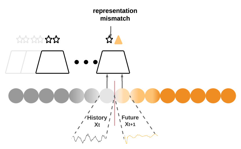
Figure 1. Overview of presented change point detection approach based on predictive representation learning.

CPD techniques have been applied to multivariate time series data in a broad range of research areas including network traffic analysis (Kurt et al., 2018), IoT applications and smart homes (Aminikhanghahi and Cook, 2019), human activity recognition (HAR) (Liono et al., 2016; Shoaib et al., 2016; Wang and Zheng, 2018; Chamroukhi et al., 2013; Deldari et al., 2020), human physiological and emotional analysis (Deldari et al., 2020), factory automation (Xia et al., 2020), trajectory prediction (Sadri et al., 2018), user authentication (Huang et al., 2019), life-logging (Chavarriaga et al., 2013), elderly rehabilitation (Lam et al., 2016), and daily work routine studies (Deldari et al., 2019). In addition to time series, CPD can applied to other data modalities with a temporal dimension, such as video, where it has been used for video captioning (Ding and Xu, 2018; Farha and Gall, 2019) and video summarising (Aakur and Sarkar, 2019; Wei et al., 2018) applications.

Change points are commonly estimated from one of a number of different properties of a time series, including its temporal continuity, distribution or shape. Unsupervised CPD methods are generally developed to identify changes based upon one particular property. For instance, FLOSS (Gharghabi et al., 2019) was developed to detect changes in the temporal shape, whilst RuLSIF (Liu et al., 2013) and aHSIC (Yamada et al., 2013) were developed to identify changes in the statistical distribution. Current CPD methods have failed to generalise effectively (Deldari et al., 2020) as the semantic boundaries of different applications will usually be associated with different time series properties. For example, abnormalities in the rhythm of the human heart are best characterised by changes in the temporal shape pattern of an electrocardiogram (ECG), whereas changes in human posture (as measured with an RFID sensor system) are best characterised by abrupt statistical changes. In this case, the detection performance degrades when a statistical CPD method is applied to the heart beat application, whilst shape based CPD methods will fail in the human posture application. Furthermore, for many applications in which data is continuously collected, time series with be characterised by slowly varying temporal shape and statistical properties. The change points associated with such time series can be subtle and remain a challenge for CPD methods to address.

In this work, we propose $TS-CP^{2}$ , a novel approach for self-supervised Time Series Change Point detection method based on Contrastive Predictive coding. We pose the question of whether self-supervised learning can be used to provide an effective, general representation for CPD. The intuition here is to exploit the local correlation present within a time series by learning a representation that maximises the shared information between contiguous time intervals, whilst minimising the shared information between pairs of time intervals that are separated in time (i.e. pairs of time intervals with less correlation). It is hypothesised that whenever the learnt representation differs significantly between time adjacent intervals, a change point is more likely to be present.

We aim to show that this self-supervised representation is capable of detecting a broader range of change points than previous methods that have been specifically designed to exploit a narrow scope of time series properties (i.e. commonly either its temporal continuity, distribution or shape patterns). Figure 1 shows a high-level overview of the approach, which is the first CPD approach based upon contrastive representation learning. Furthermore, whilst there are contrastive learning methods for image (Chen et al., 2020; Sohn, 2016), audio (Oord et al., 2018; Saeed et al., 2020) and text (Oord et al., 2018), this is the first approach utilising contrastive learning on general time series, which in turn, introduces some unique challenges. Furthermore, our technique does not rely on any assumptions about the statistical distribution of the data making it applicable to a broad range of real-world applications. The main contributions of our paper are as follows:

• We leverage contrastive learning as an unsupervised objective function for the CPD task. To the best of our knowledge, we are the first to employ contrastive learning to the CPD problem.

• We propose a representation learning framework to tackle the problem of self-supervised CPD by capturing compact, latent embeddings that represent historical and future time intervals of the times series.

• We compare our proposed method against five state of the art CPD methods, which include deep learning and non deep learning based methods, investigate the benefits of each through extensive experiments.

• We investigate the performance impact of the hyperparameters used within our self-supervised learning method including batch size, code size, and window size.

To make $TS-CP^{2}$ reproducible, all the code, data and experiments are available in the project’s web page .

2. Related Work and Background

In this section, we review existing approaches for the CPD problem. Since we employ contrastive learning for our time series change point detection method, we also outline recent works on self-supervised contrastive learning. We will then review recent representation learning approaches, not only for time series data, but other data modalities as well.

2.1. Time series change point detection

Although self-supervised learning methods have recently attracted the interest of the deep learning community, current CPD methods are mostly based on non deep learning approaches yet.

Existing approaches can be categorised based upon the features of the time series that they consider for CPD. Statistical methods often compute change points on the basis of identifying statistical differences between adjacent short intervals of a time series. The statistical differences between intervals are usually measured with either parametric or non-parametric approaches. Parametric methods use a Probability Density Function (PDF) such as (Basseville and Nikiforov, 1993) or auto-regressive model (Yamanishi and Takeuchi, 2002) to represent the time intervals, however, such convenient representations limit the types of statistical changes that can be detected. Non-parametric methods offer a greater degree of flexibility to represent the density functions of time intervals by utilising kernel functions. Estimating the ratio of time interval PDFs is a simpler problem to address than estimating the individual PDFs of the time intervals. The methods in RuLSIF (Liu et al., 2013), KLIEP (Yoshinobu and Sugiyama, 2012) and SEP (Aminikhanghahi and Cook, 2019) used a non-parametric Gaussian kernel to model the density ratio distribution between subsequent time intervals. (Yamada et al., 2013) detected abrupt change points by calculating separability of adjacent intervals based on kernel-based additive Hilbert-Schmidt Independence Criterion (aHSIC). Kernel approaches assume there is statistical homogeneity within each interval, which can be problematic for change point detection. Furthermore, kernel functions often require parameters to be carefully tuned.

There is another category of statistical CPD approaches that identify change points as the segment boundaries that optimise a statistical cost function across the segmented time series. IGTS (Sadri et al., 2017) and OnlineIGTS (Zameni et al., 2019) estimated change points by proposing top-down and dynamic programming approaches to search for the boundaries that maximised the information gain of the segmented time series. GGS (Hallac et al., 2019) proposed an online CPD approach that used a greedy search to identify the boundaries that maximised the regularised likelihood estimate of the segmented Gaussian model.

Another broad category of CPD methods exploit the temporal shape patterns of time series. FLOSS was proposed to detect change points by identifying the positions within the time series associated with a salient change in its shape patterns (Gharghabi et al., 2019). Authors of (Xia et al., 2020) proposed a motif discovery approach in order to extract rare patterns that can distinguish separate segments (Huang et al., 2014). Recently, ESPRESSO (Deldari et al., 2020) proposed a hybrid CPD approach that exploit both the temporal shape pattern and statistical distribution of time series. It was shown that the hybrid model was able to detect change points across a diverse range of time series datasets with greater accuracy than purely statistical or temporal shape based methods.

Deep learning based CPD methods have also recently been proposed. The authors of (De Ryck et al., 2020) used an AutoEncoder for CPD by exploiting peaks in the reconstruction error of the encoded representation. Kernel Learning Change Point Detection, KL-CPD (Chang et al., 2019), is a state-of-the-art end-to-end CPD method which solves the problem of parameter tuning in kernel-based methods, by automatically learning the kernel parameters and combining multiple kernels to capture different types of change points. KL-CPD utilised a two-sample test for measuring the difference between contiguous sub-sequences. KL-CPD was shown to significantly outperform other deep learning and non deep learning CPD methods.

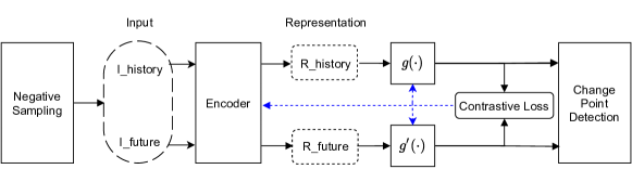
Figure 2. Illustration of the overall architecture of our $TS-CP^{2}$. Blue dash arrows indicate the back propagation in the training phase.

CPD is also useful in video processing applications for summarising video, extracting segments of interest (Wei et al., 2018), and automatic caption generation and synchronisation (Aakur and Sarkar, 2019; Ding and Xu, 2018; Farha and Gall, 2019). Existing video segmentation approaches are commonly supervised and benefit from having knowledge of the order of actions. In contrast, (Aakur and Sarkar, 2019) proposed an auto-regressive model to predict the next video frames based on the most recently seen frames. Abrupt increases in the prediction error were then used to detect the segment boundaries.

2.2. Representation Learning

In recent years, self-supervised representation learning has been used to capture informative and compact representations of video (Aakur and Sarkar, 2019; Mounir et al., 2020), image (Chen et al., 2020; Hénaff et al., 2020), text(Oord et al., 2018), and time series (Saeed et al., 2019; Lu and Huang, 2020; Saeed et al., 2020; Franceschi et al., 2019) data.

2.2.1. Contrastive Learning

Contrastive learning is an approach used to formulate what makes the samples in a dataset similar or dissimilar using a set of training instances composed of positive sample pairs (samples considered to be similar in some sense) and negative sample pairs (samples considered to be different). A representation is learnt to bring the positive sample pairs closer together and to further separate negative sample pairs within the embedding space. Contrastive loss (Chopra et al., 2005) and Triplet loss (Weinberger and Saul, 2009) are the most commonly used loss functions. In general, the triplet loss function outperforms the contrastive loss function because it considers the relationship between positive and negative pairs, whereas the positive and negative pairs are considered separately in the contrastive loss function. Triplet loss, however, only considers one positive and one negative pair of instances at a time. Both functions suffer from slow convergence and require expensive data sampling methods to provide informative instance pairs, or triplets of instances, that accelerate training (Sohn, 2016). To solve the aforementioned problems, Multiple Negative Learning loss functions have been proposed to consider multiple negative sample pairs simultaneously. N-Paired loss (Sohn, 2016) and infoNCE based on Noise Contrastive Estimation (Gutmann and Hyvärinen, 2010; Mnih and Kavukcuoglu, 2013) are examples of recent multiple negative learning loss functions. These approaches, however, require computationally expensive sampling approaches to select negative sample instances for training. This issue of complexity has been addressed by Hard Negative Instance Mining, which has been shown to play a critical role in ensuring contrastive cost functions are more efficient (Duan et al., 2019; Wu et al., 2017). A number of sampling strategies have been proposed, including hard negative sampling (Simo-Serra et al., 2015), semi-hard mining (Schroff et al., 2015), distance weighted sampling (Wu et al., 2017), hard negative class mining (Sohn, 2016), and rank-based negative mining (Wang et al., 2019).

2.2.2. Contrastive-based Representation Learning

Most existing work on representation learning focus upon natural language processing (Oord et al., 2018) and computer vision (Chen et al., 2020; Hénaff et al., 2020) domains. Howerver, to the best of our knowledge, it is the first time contrastive learning has been used for change point detection.

There is a few works that investigates the use of representation learning with multivariate time series. The authors of (Franceschi et al., 2019) proposed a general-purpose approach to learn representations of variable length time series using a deep dilated convolutional network (WaveNet (Oord et al., 2016)) and an unsupervised triplet loss function based on negative sampling.

Contrastive predictive coding, CPC (Oord et al., 2018), uses auto-regressive models to learn representations within a latent embedding space. The aim of CPC is to learn within an abstract, global representation of the signal as opposed to a high dimension, lower level representation. The authors demonstrated it could learn effective representations of different data modalities such as images, text and speech for downstream modelling tasks. Firstly, a deep network encoder was used to map the signal into a lower dimension latent space before an auto-regressive model was then applied to predict future frames. A contrastive loss function maximised the mutual information between the density ratio of the current and future frames. CPCv2 (Hénaff et al., 2020) replaced the auto-regressive RNN of CPC with a convolutional neural network (CNN) to improve the quality of the learnt representations for image classification tasks.

3. Method

3.1. Problem Definition

Given a multivariate time series $\{X_{1},X_{2},...,X_{T}\}$ of $T$ observations, where the vector $X_{i}\in\mathbb{R}^{d}$, we attempt to estimate the times ($t$) that are associated with a change in the time series properties. We define change points (or segment boundaries) as the time points in future can not be anticipated from the data before this point. Hence, the dissimilarity between future representation and anticipated representations can be used as a measure to detect transition to the next segment.

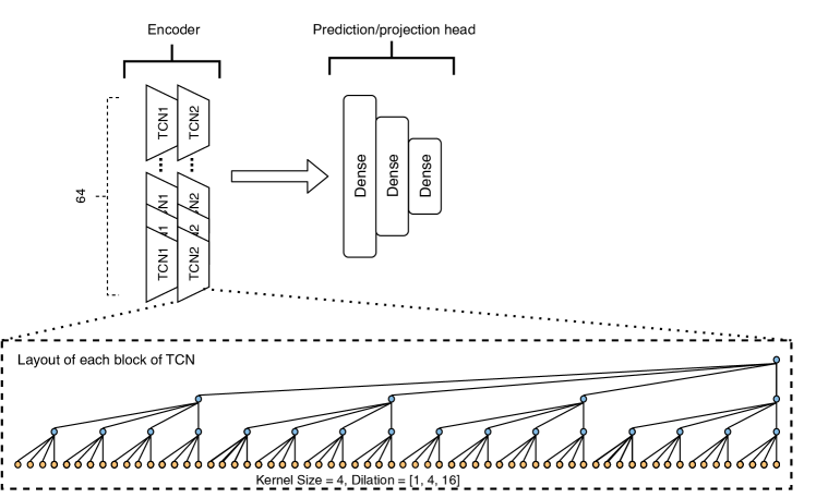
Figure 3. The encoder architecture for $TS-CP^{2}$Ẇe use two stacks of TCN with kernel size 4 and dilation sizes of 1, 4, and 16 followed by three Dense layers as the prediction head.

3.2. $TS-CP^{2}$  Overview

There are change point and temporal anomaly detection methods for video (Aakur and Sarkar, 2019) and time series (Kokkonen et al., 2019) that use an auto-regressive model for prediction. In these approaches, change points are detected at samples associated with a salient increase in the prediction error. However, since the prediction error is highly dependent upon the distribution of the data, we propose to use representation learning to extract a compact latent representation that is invariant to the original distribution of the data. Figure 1 illustrates the main idea behind our $TS-CP^{2}$ approach. We hypothesize that this approach is much more effective to detect change points because the embedding space that is extracted from contiguous time intervals are likely to be dependent upon the same shared information.

Here we adopt a similar approach to the CPC (Oord et al., 2018; Hénaff et al., 2020) method to learn a representation that maximises the mutual information between consecutive time windows. Firstly, an auto-regressive deep convolution network, WaveNet (Oord et al., 2016), was employed to encode each of the time series windows. Secondly, a 3-layer fully connected network was employed on top of this encoding to produce a more compact, embedded representation. The cosine similarity was computed between the embeddings of consecutive time windows in order to estimate the change points. The time intervals associated with smaller similarity values had a higher likelihood of being change points. A contrastive learning approach was used to train the encoder by using a single pair of contiguous time windows (positive pair) and a set of window pairs that were separated across time (negative pairs) within each batch.

We applied the $N-pairedloss$ metric (Sohn, 2016) (which is described in section 3.3.1) to maximise the mutual information between the positive pairs amongst the set of negative pairs of samples.

Figure 2 shows the overall architecture of the proposed method. In the following section we will describe the main modules in the following order: 1) Representation learning, 2) Negative sampling, and 3) Change point detection.

3.3. Representation Learning

At the core of the $TS-CP^{2}$ approach is an encoder that maps pairs of contiguous time windows into a compact embedding representation. This representation was trained to learn about the concept of similarity over short temporal scales by maximising the mutual information between the pairs of adjacent time windows. We employ the auto-regressive deep convolution network, WaveNet (Oord et al., 2016), to learn our encoded representation. We do not use an LSTM to encode the time series, given it has been shown that temporal convolutional networks (TCN) can often produce superior prediction performance with sequential data (Hénaff et al., 2020) and are generally easier to train.

Figure 3 illustrates the encoder architectures. It consists of two blocks of TCN with 64 kernel filters of size 4 and three layers of dilation with respective rates of 1, 4 and 16. The TCN is then followed by a simple three-layer projection head with ReLU activation function and batch normalisation. The modified illustration of TCN layer is shown in the figure.

Pairs of history and future time windows are fed into an encoder. A projection head is used (shown as $g(\cdot)$ and $g^{\prime}(\cdot)$ in Figure 2, respectively) to map each window encoding into a lower dimension space. To this end, an MLP neural network with three hidden layers was used.

Contrastive learning used pairs of history and future windows for training an embedded representation. Two different types of time window pairs were contrasted for training. Each training instance was comprised of a positive sample pair of contiguous time intervals and a set of negative sample pairs with intervals separated across time. In the next subsection, we define the $InfoNCE$ cost function that will be used for representation learning.

3.3.1. Cost function

We applied the $InfoNCE$ loss function that is based upon Noise Contrastive Estimation (Mnih and Kavukcuoglu, 2013), which was originally proposed for natural language representations but has also recently been adopted for image representation learning techniques (Hénaff et al., 2020; Oord et al., 2018; Chen et al., 2020).

The $InfoNCE$ cost function is defined to maximise the mutual information between consecutive time windows. A single positive pair of time adjacent intervals $(h_{i},f_{i})$, the history window (${h_{i}}$) and future window (${f_{i}}$), and a set of $K-1$ negative pairs ($(h_{i},f_{j})_{j\neq i}$) where the intervals ${h_{i}}$ and ${f_{j}}$ were well separated in time across the sequence.

Using the $InfoNCE$ loss function, we calculate the probability $\rho_{i}$ of the positive sample pair in each batch using the scaled-$Softmax$ function:

(1) $$\rho_{i}={\frac{exp(Sim(h_{i},f_{i})/\tau)}{\sum_{j=1}^{K}{exp(Sim(h_{i},f_{j})/\tau)}}}\$$

where ${\tau}$ is a scaling parameter and $Sim$ is the cosine similarity between each pair of data embeddings. The final loss is calculated with the binary cross-entropy function over the probabilities of all $K$ positive pairs belonging to the training batch. Since the probabilities of the positive sample pairs are computed using the similarity scores of the negative sample pairs in (1), the cross entropy loss function can be simplified to:

(2) $$\mathbf{\mathscr{L}}=-\sum_{i,j}{y_{ij}log(\rho_{i})+(1-y_{ij})log(1-\rho_{i})}$$

(3) $$\centering\mathscr{y}_{ij}=\begin{cases}1&\text{if $i=j$}\\ 0&\text{if $i\neq j$}\\ \end{cases}\@add@centering$$

(4) $$\mathbf{\mathscr{L}}=\sum_{i}{-log(\rho_{i})}$$

3.3.2. Negative Sampling

Following on from the hard negative class mining approach in (Sohn, 2016), we propose a simpler sampling strategy where positive sample pairs are randomly sampled and used to construct the negative sample pairs for each batch. Figure 4 depicts the process of batch construction in our model. We choose $K$ random pairs of contiguous windows $(h_{i},f_{i})$ as the positive pairs in each training batch. Each pair must adhere to the constraint of being a minimum temporal distance from the other pairs. This minimum temporal distance constraint is used to enable each batch to adopt the future windows of the other $K-1$ positive pairs as negative pairs, given they are guaranteed to be sufficiently separated from the history window in the batch’s own positive pair. The intuition is that time series are commonly non-stationary, and hence, windows that are temporally separate from one another are likely to exhibit far weaker statistical dependencies than adjacent windows. We need to set the threshold of minimum temporal distance based upon the time series application being considered.

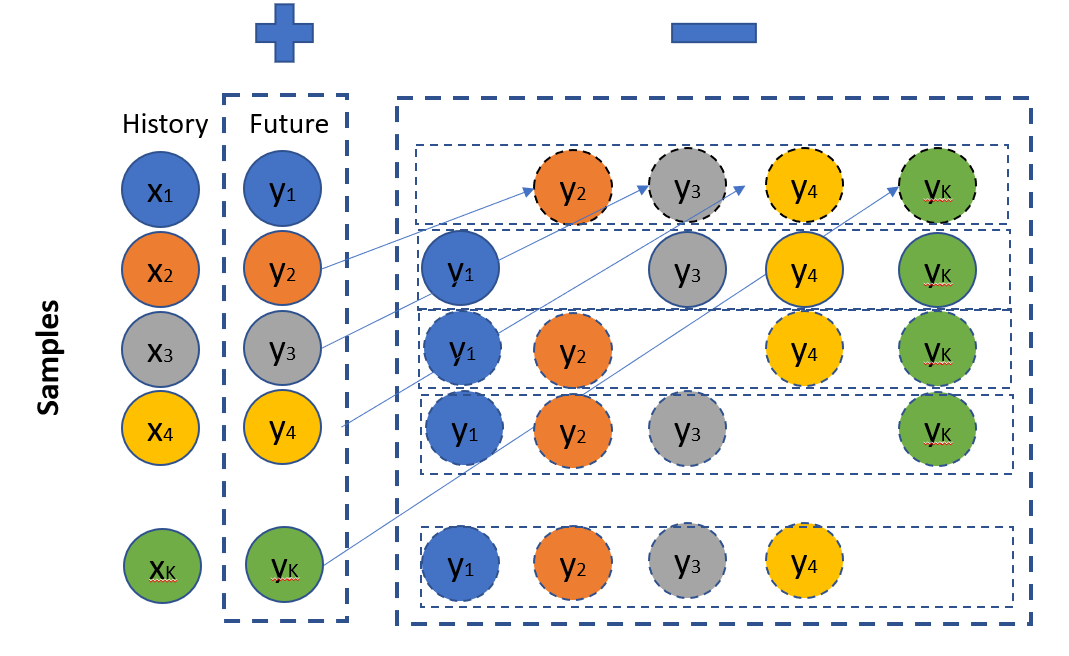
Figure 4. Batch construction

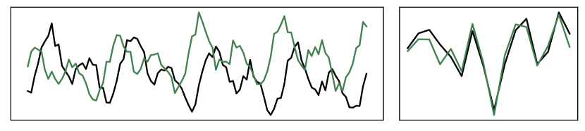
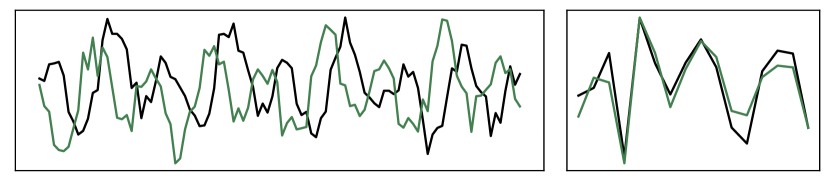
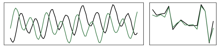
Figure 5. Three examples of positive pairs of samples (left, length = 100) and their corresponding embedding (right, length = 16). The positive pairs are subsequent intervals of the time series.

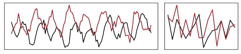
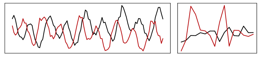
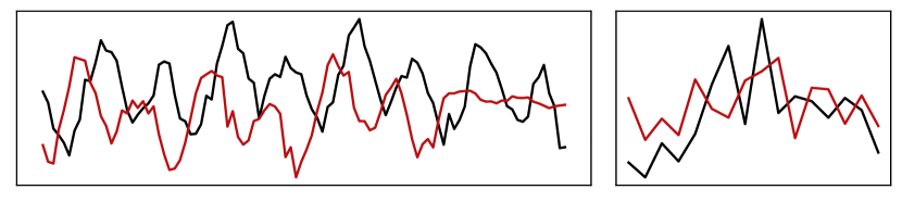
Figure 6. Three examples of negative pairs of samples (left, length = 100) and their corresponding embedding (right, length = 16). The negative pairs correspond to time intervals of the time series that well separated in time. A change point or anomaly has occurred somewhere in either history or future frame of the negative pairs.

Consequently, we can select positive and negative sample pairs with a relatively low complexity relative to the other negative mining approaches mentioned in Section 2. Figure 6 and 6 show examples of time windows belonging to the positive and negative pairs, respectively, and their corresponding embedding vectors.

3.4. Change Point Detection Module

We hypothesize that when a change point intersects a pair of history and future windows, their associated embeddings will be distributed differently. Consequently, in order to detect change points from the time series being tested, we transform pairs of history and future windows into a compact embedding and compute the cosine similarity ($Sim(h_{i},f_{i})$) between the embedding pairs across the time series being tested. The difference between the cosine similarity and moving average of the cosine similarity was computed and a peak finding algorithm was applied to find local maxima in the difference function (increase in difference function is associated with decrease in similarity metric). The time intervals associated with these local maxima are considered as the change point estimates.

Figure 7 shows an example of the cosine similarity between the latent embeddings of the history and future windows within a time series. The green areas show the interval pairs $(h_{i},f_{i})$ which contain a change point for a subset of the Benchmark-4 of the Yahoo! dataset (Dataset, [n.d.]). It is clear that the local minima of the difference between the cosine similarity of each interval pair $(h_{i},f_{i})$ and the average similarity across recent intervals pairs coincide with true change points.

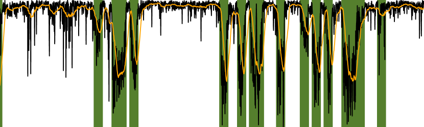
Figure 7. An example of detecting change points based upon the cosine similarity between consecutive window pairs. The black line shows the cosine similarity between subsequent time intervals in Benchmark-4 of the Yahoo! dataset (Dataset, [n.d.]). The green areas highlight the intervals with change points and the yellow line shows the moving average of the cosine similarity for the previous $W$ intervals.

4. Experiments

In this section, we present our evaluation of the proposed $TS-CP^{2}$ method. Firstly, we introduce the datasets and outline the baseline CPD methods used in our experiments. A sensitivity analysis of the $TS-CP^{2}$ method is presented along with a performance comparison with baseline CPD methods. $TS-CP^{2}$ is implemented using Tensorflow 2.2.0 and python 3.7.2.

4.1. Datasets

We show the effectiveness of our method across a diverse range of applications that include web service traffic analysis, human activity recognition and mobile application usage analysis.

• Yahoo!Benchmark (Dataset, [n.d.]). The Yahoo! benchmark dataset is one of the most widely cited benchmarks for anomaly detection. It contains time series with varying trend, seasonality, and noise including random anomaly change points. We used all 100 time series of the fourth benchmark, as it is the only portion of the dataset that includes change points.

• HASC (Kawaguchi et al., 2011a; Kawaguchi et al., 2011b). The HASC challenge 2011 dataset provides human activity data collected by multiple sensors including an accelerometer and gyrometer. We used a subset of the HASC dataset (The same subset used by recent state-of-the-art method, KL-CPD) including only 3-axis accelerometer recordings. The aim of detecting change point detection with this dataset is to find transitions between physical activities such as ”stay”, ”walk”, ”jog”, ”skip”, ”stair up”, ”stair down”.

• USC-HAD (Zhang and Sawchuk, 2012). USC-HAD dataset includes twelve human activities that were recorded separately across multiple subjects. Each human subject was fitted with a 3-axis accelerometer and 3-axis gyrometer that were attached to the front of the right hip and sampled at 100Hz. Activities were repeated five times for each subject and consisted of: ”walking forward”, ”walking left”, ”walking right”, ”walking upstairs”, ”walking downstairs”, ”running forward”, ”jumping up”, ”sitting”, ”standing”, ”sleeping”, ”elevator up”, and ”elevator down”. We randomly chose 30 activities from the first six participants and stitched the selected recordings together in a random manner. In the experiments undertaken in this paper, only the data from the accelerometer was used.

Table 1 outlines the properties of each dataset.

Table 1. The properties of the three datasets used in our experiments. T is the total number of samples, #sequences is the quantity of time series, #channels represents the time series dimensionality and #CP is the total number of change points in each dataset.

dataset	T	#sequences	#channels	#CP
Yahoo! Benchmark	164K	100	1	208
HASC	39K	1	3	65
USC-HAD	97K	6	3	30

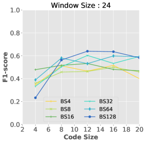
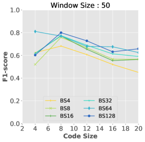
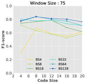
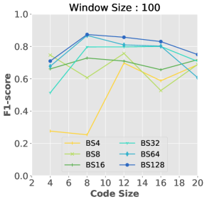
Figure 8. A sensitivity analysis of the the Yahoo!Benchmark dataset with respect to the code size, batch size and four window sizes of: (a) 24 samples (b) 50 samples (c) 75 samples and (d) 100 samples.

4.2. Baseline Methods

The performance of the proposed $TS-CP^{2}$ method was compared against five state-of-the-art unsupervised change point detection techniques that included ESPRESSO (Deldari et al., 2020), FLOSS (Gharghabi et al., 2019), aHSIC (Yamada et al., 2013), RuLSIF (Liu et al., 2013), and KL-CPD (Chang et al., 2019). To avoid inconsistencies and implementation errors, and to provide a fair comparison, baseline methods were evaluated using the publicly available source code.

Kernel specific parameters were used by the RuLSIF and aHSIC methods. For RuLSIF, the regularisation constant was set to a value of 0.01, as suggested in (Liu et al., 2013). For aHSIC, the regularisation constant and the kernel bandwidth parameters were set to values of 0.01 and 1, respectively, as specified in (Yamada et al., 2013).

Detection performance was compared across a range of window sizes that were unique to each dataset based on its sampling rate. As a deep learning based method, KL-CPD required several hyper-parameters to be tuned; window size, batch size and learning rate. To enable a fair comparison with the other methods, a grid search was performed across the sets of hyper-parameter values. Only the hyper-parameter configuration that provided the highest rate of true positives was presented. We used the same evaluation approach as undertaken with KL-CPD to calculate the F1-score. The remaining parameters were set according to the values specified in (Chang et al., 2019). Although the training process of KL-CPD was unsupervised, the method still required ground truth labels to be used to fine-tune the model hyper-parameters during the validation phase. For the FLOSS and ESPRESSO methods, we used the z-normalised euclidean distance as the similarity metric, as suggested by authors of their underlying structure they used in (Zhu et al., 2016).

4.3. Evaluation Metrics

The performance of models were evaluated with respect to the F1-score. The error margin in which a change point can be detected is an important factor in evaluating the performance of each CPD method (Aminikhanghahi and Cook, 2017). Hence, we report the F1-scores of each dataset for the three different detection margins specified in Table 2.

Each change point estimate was defined as a true positive when it was located within the specified error margin of the ground truth change point. When multiple change point estimates were located within the error margin of the the ground truth change point, only the closest estimate was considered to be a true positive. The remaining estimates were considered to be false positives. Ground truth change points without any estimates that fell within the specified error margin were considered to be false negatives.

4.4. Fine-Tuning and Sensitivity Analysis

In this section, we have done extensive experiments to analyse the sensitivity of our proposed method to:

• Window size is the length of the history and future intervals. We consider a range of values that are dependent upon the particular application and sampling rate of the dataset. The window size should be large enough to encapsulate the properties of the time series but not too large to encompass multiple change points. We select window sizes of 1,2,3 and 4 days for the Yahoo!Benchmark dataset and 0.5,1,2 and 4 seconds for the HAR dataset.

• Batch Size specifies the number of training instances ($K$) that were processed before the model was updated. It also specifies the number of negative pairs ($K-1$) used in each training instance. The batch size was selected to range between 4 and 128 samples.

• Code Size specifies the length of the embedding vector that is extracted from the encoder network. The range of code sizes that were selected ranged between 4 to 20 dimensions.

Window size is the only input parameter to investigate for the ESPRESSO and FLOSS methods and the main parameter for the RulSIF and aHSIC methods. For the deep learning based methods, including the proposed method, we also investigate the performance of a number of parameters including the window size, batch size, code size and learning rate. Figure 8 compares the $TS-CP^{2}$ performance (with respect to the F1-score) for the Yahoo!Benchmark dataset across the different parameter settings.

4.4.1. Window size

Since the Yahoo!Benchmark dataset is sampled hourly and the minimum length between two consecutive change points is approximately 160 samples, we consider a range of window sizes between 24 (1 day) to 100 ( 4 days). Figure 8 shows there was a monotonic increasing relationship between the window size and detection performance averaged across the code size and batch size. It was hypothesized that longer windows possess the highest F1 scores, given they encapsulate additional properties of the time series into modelling.

4.4.2. Batch Size

We varied the batch size with respect to the set of $\{4,8,16,32,64,128\}$ dimensions to investigate its impact upon detection performance. Figure 8 shows there was a monotonic increasing relation between the batch size and detection performance when averaged across the code size and window size. There are particular situations for the smallest code size, however, where the largest batch sizes had inferior detection performance to the smaller batch sizes. We hypothesize such situations can occur given larger batches are more likely to generate false negative samples from the time series datasets and smaller code size are too short to represent all informative features of data. False pairs of negative samples are pairs of time windows that are considered to be false instances, but are found to be similarly distributed. Whilst the negative sample pairs are constrained to be intervals that are temporally separate from one another, time series are often comprised of patterns (and their associated semantic classes) that repeat at different, non-contiguous positions within the sequence. Consequently, using contrastive learning to separate these false pairs of negative samples within the embedding space can degrade detection performance.

4.4.3. Code Size

In contrast to many representation learning approaches, we investigated how the embedding dimensionality affected the detection performance. We varied the code size from 4 to 20 dimensions which equates to representing between 4% to 83% of a window from the experiment. As shown in Figure 8, the optimal code size was dependent upon the window size and batch size. In general, the smallest code size of 4 showed a relatively weak performance for each of the window sizes, given there was insufficient capacity to represent the key features of the time series to learn an effective representation. The relationship between detection performance and code size was not monontonic increasing, however, given the largest code sizes were often shown to be inferior to the more compact embeddings with a code size of between 8 and 12 dimensions.

Table 2. The performance of the proposed $TS-CP^{2}$ method was compared to the other baselines methods across the Yahoo!Benchmark, HASC, and USC datasets. The bold and underlined texts represent the methods with the first and second highest F1-scores, respectively. The detection margin is the maximum number of samples that an estimated change point can be from a ground truth change point to still be considered a True Positive. We present the highest F1-score of each method (for the best window size) and the F1-score of the methods averaged across all window sizes.

Dataset	Detection margin	24		50		75
	Methods	Best Wnd	F1-score	Best Wnd	F1-score	Best Wnd	F1-score
Yahoo	FLOSS	45	0.2083	50	0.3375	55	0.4233
	aHSIC	40	0.4092	40	0.4175	40	0.4392
	RuLSIF	20	0.3175	20	0.3317	20	0.3700
	ESPRESSO	50	0.2242	50	0.3400	70	0.4442
	KL-CPD	24	0.5787	50	0.5760	75	0.5441
$TS-CP^{2}$	24	0.64	50	0.8104	75	0.8428
USC	Detection margin	100		200		400
	FLOSS	100	0.2666	100	0.3666	400	0.4333
	aHSIC	50	0.3333	50	0.3333	50	0.3999
	RuLSIF	400	0.4666	400	0.4666	400	0.5333
	ESPRESSO	100	0.6333	100	0.8333	100	0.8333
	KL-CPD	win:100, bs:4	0.7426	win:200,bs:32	0.7180	win:400,bs:16	0.6321
$TS-CP^{2}$	win:100, bs:8	0.8235	win:200, bs:8	0.8571	win:400, bs:32	0.8333
HASC	Detection margin	60		100		200
	FLOSS	60	0.3088	60	0.3913	100	0.5430
	aHSIC	40	0.2308	40	0.3134	40	0.4167
	RuLSIF	200	0.3433	200	0.4999	200	0.4999
	ESPRESSO	100	0.2879	60	0.4233	100	0.6933
	KL-CPD	win:60,bs:4	0.4785	win:100,bs:4	0.4726	win:200,bs:64	0.4669
$TS-CP^{2}$	win:60,bs:64	0.40	win:100,bs:64	0.4375	win:200,bs:64	0.6316

4.5. Baseline Comparison

The performance of the proposed $TS-CP^{2}$ method was compared to the five baseline methods across the three datasets. To enable a fair comparison between the methods, we performed a grid search of the set of parameters associated with each method. For each method, the model with the best F1-score and its corresponding parameters were presented in Table 2.

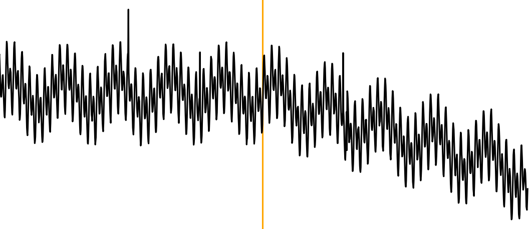
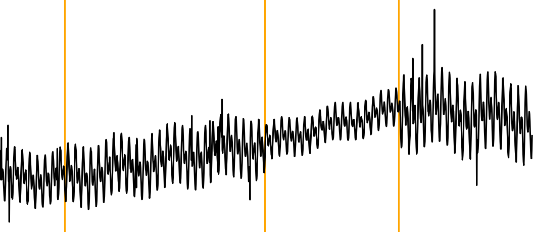
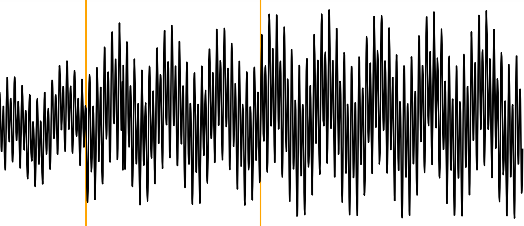
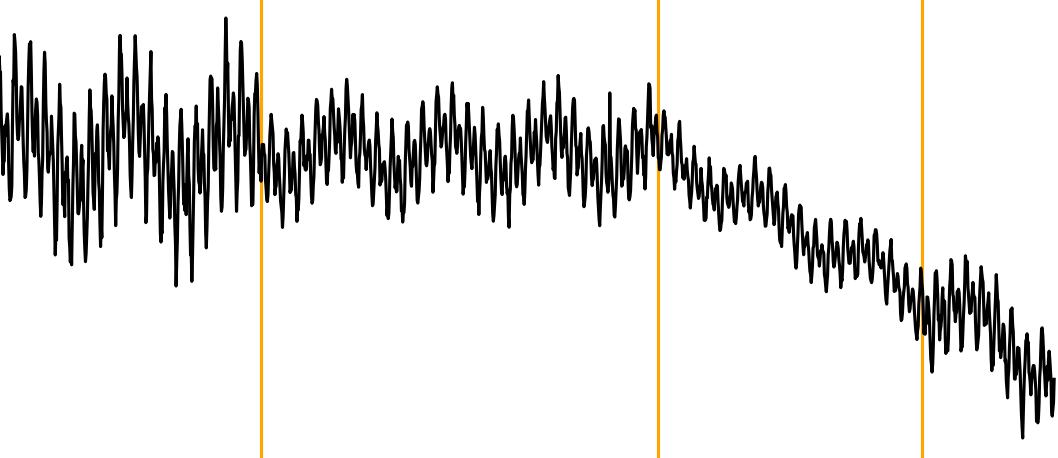
Figure 9. Four random time series from the Yahoo! Benchmark dataset. The yellow vertical lines correspond to the change points. The spatial anomalies are not highlighted as they are not the focus of the experiment.

4.5.1. Yahoo! Benchmark Evaluation

To compare the ability of each method to detect change points, we set three different detection error margins of 24, 50, and 75 samples. If the difference between the actual and estimated change points were less than the specified margin, it was considered to be a true positive. Table 2 shows the highest F1-score and corresponding window size for each method.

The Yahoo! Benchmark dataset is well-cited (according to (Wu and Keogh, 2020)) and one of the more complex datasets for temporal anomaly detection given the anomalies are mostly based upon changes in the seasonality, trend and noise. Based on the results reported in Table 2, our proposed method $TS-CP^{2}$  strongly outperforms each of the other baseline methods.

Although all of the baselines are state-of-the-art methods for CPD, this dataset was shown to be challenging for them. Four randomly selected sequences of this dataset are illustrated in Figure 9. $FLOSS$ and $aHSIC$ were able to detect changes in temporal shape patterns, however, they could not distinguish the change points associated with subtle statistical differences. $RuLSIF$ estimate change points based upon the difference in the ratio of the distributions of adjacent time intervals. It was clear for some of the change points of the sequences in Figure 9 that adjacent segments were similarly distributed and only exhibited clear changes in their temporal shape.

4.5.2. USC-HAD Dataset Evaluation

Given the sampling rate for this dataset is 100Hz, the maximum error margins for which a change point estimate was considered to be a true positive was 1, 2, and 4 seconds. We investigate different values of the kernel bandwidth for RuLSIF and different kernel sizes (20, 40, and 50) for aHSIC. Different window size were investigated for FLOSS, ESPRESSO, KL-CPD, and $TS-CP^{2}$ as they were varied between 100, 200, and 400 samples. We also used different learning rates for KL-CPD and $TS-CP^{2}$ of $3\times 10^{-4}$ and $1\times 10^{-4}$, respectively.

As shown in Table 2, our proposed method outperformed the other baselines across each of the error margins. $TS-CP^{2}$ is the only method that delivers a high F1-score for the smallest error (100 samples) meaning it can reliably detect change points within one second of its occurrence.

Similarly to the Yahoo! Benchmark dataset, we compare the effect of batch size across the different window sizes for $TS-CP^{2}$ in Figure 10. It was shown that larger batch sizes offered a superior detection performance across the longer windows. The shorter batch sizes, however, were shown to offer superior detection performance across the smaller windows.

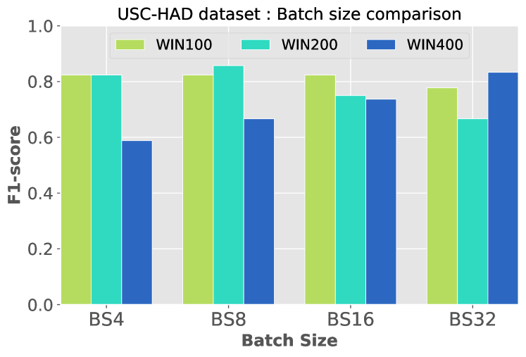
Figure 10. Comparing the effect of batch size across different window sizes for USC-HAD dataset.

4.5.3. HASC dataset Evaluation

The HASC dataset was found to be the most challenging dataset for $TS-CP^{2}$ and the other baseline methods. Although $TS-CP^{2}$ achieves the second highest performance level with respect to each of the different window sizes, it still achieves the highest average F1-score with a 19.2%, 54.8%, 10.1%, 11.1%, and 3.8% improvement over FLOSS, aHSIC, RulSIF, ESPRESSO, and KL-CPD, respectively.

The HASC dataset is the smallest in size (around 39K samples) but contains the largest number of change points (65 change points in total). Consequently, the relatively high density of change points means there there is a greater likelihood to generate positive sample pairs that encompass change points. Such false positive sample pairs will degrade model training. Since the model is self-supervised, ground truth labels cannot be used to rectify any such errors with positive sample pairs. Consequently, to address this problem, we suggest to enhance the model by injecting a light negative mining. We could also generate more positive sample pairs through augmentation.

4.5.4. Discussion

We showed that $TS-CP^{2}$ was able to outperform non deep learning based methods, FLOSS, aHSIC, RulSIF and ESPRESSO, by 104.3%, 91.0%, 68.9%, 53.3% and 24.9% improvement with respect to the F1-score averaged over all of the datasets. In addition, $TS-CP^{2}$ showed a 17.0% improvement in F1-score over KL-CDP, which is the most recent and competitive deep-learning-based change point detection method.

Since the baseline CPD methods exploit abrupt changes in one particular property of the time series, they do not effectively generalise to different types of datasets. For example, the hybrid ESPRESSO method performs well on the USC-HAD dataset, given its change points are commonly associated with abrupt changes in both its temporal shape and statistical properties. But neither ESPRESSO nor the other non deep learning approaches were as effective in estimating change points associated with the Yahoo!Benchmark given its change points were composed of more subtle and slowly evolving transitions in properties. In contrast, we showed that our proposed $TS-CP^{2}$ method achieved either the first or second highest result across each of the datasets. $TS-CP^{2}$ showed a significant improvement over the five baselines for the Yahoo! and USC-HAD datasets, whilst its average performance across the different window sizes was superior to each baseline with the HASC dataset.

In future work, we will investigate using augmentation and negative mining batch construction to address the problem of high frequency change points that present themselves in some of the datasets discussed in section 4.5.3.

Finally, $TS-CP^{2}$ employs a compact structure with a shared representation to encode its history and future windows. This enables faster training convergence compared to its other deep learning counterpart, KL-CPD. Furthermore, once the representation model is trained, CPD is very simple to implement given it only involves a comparison between the learnt representations of the history and future windows. Consequently it has the potential to be implemented for online operation on low resource devices. The baseline methods (other than the FLOSS method which has introduced a streaming version) cannot be applied online as they need to consider a reasonably large batch of data to capture repeated patterns or to optimise the entropy-based loss function.

5. Conclusion

We propose a novel self-supervised CPD method, $TS-CP^{2}$  for time series. $TS-CP^{2}$ learns an embedded representation predict a future interval of a times series from historical samples. Change points are detected at the times in which the embedded are relatively high. Our proposed method is the first CPD method that employs contrastive learning to extract a compact and informative representation vector for every frame and estimate the change point based on the agreement between the learnt representation of subsequent frames.

We evaluated the ability of $TS-CP^{2}$ in detecting change points against six other well-known state-of-the-art methods across three datasets. We have shown that our proposed method significantly outperform other baselines in two dataset and reaches a comparable score for the other dataset. Although the pre-trained $TS-CP^{2}$ can detect changes in online applications, we aim to expand this method in our future work to continuously learn changes, anomalies and drifts in data.

- (1)
- Aakur and Sarkar (2019) Sathyanarayanan N Aakur and Sudeep Sarkar. 2019. A Perceptual Prediction Framework for Self Supervised Event Segmentation. In Proceedings of the IEEE Conference on Computer Vision and Pattern Recognition. 1197–1206.
- Aminikhanghahi and Cook (2017) Samaneh Aminikhanghahi and Diane J. Cook. 2017. A Survey of Methods for Time Series Change Point Detection. Knowledge and information systems 51, 2 (01 May 2017), 339–367.
- Aminikhanghahi and Cook (2019) Samaneh Aminikhanghahi and Diane J Cook. 2019. Enhancing Activity Recognition Using CPD-based Activity Segmentation. Pervasive and Mobile Computing 53 (2019).
- Basseville and Nikiforov (1993) Michelle Basseville and Igor V Nikiforov. 1993. Detection of abrupt changes: theory and application. Prentice Hall.
- Chamroukhi et al. (2013) Faicel Chamroukhi, Samer Mohammed, Dorra Trabelsi, Latifa Oukhellou, and Yacine Amirat. 2013. Joint Segmentation of Multivariate Time Series with Hidden Process Regression for Human Activity Recognition. Neurocomputing 120 (2013), 633–644.
- Chang et al. (2019) Wei-Cheng Chang, Chun-Liang Li, Yiming Yang, and Barnabás Póczos. 2019. Kernel change-point detection with auxiliary deep generative models. arXiv preprint arXiv:1901.06077 (2019).
- Chavarriaga et al. (2013) Ricardo Chavarriaga, Hesam Sagha, Alberto Calatroni, Sundara Tejaswi Digumarti, Gerhard Tröster, José del R Millán, and Daniel Roggen. 2013. The Opportunity challenge: A benchmark Database for On-Body Sensor-based Activity Recognition. Pattern Recognition Letters 34, 15 (2013), 2033–2042.
- Chen et al. (2020) Ting Chen, Simon Kornblith, Mohammad Norouzi, and Geoffrey Hinton. 2020. A Simple Framework for Contrastive Learning of Visual Representations. ICML (2020).
- Chopra et al. (2005) Sumit Chopra, Raia Hadsell, and Yann LeCun. 2005. Learning a similarity metric discriminatively, with application to face verification. In 2005 IEEE Computer Society Conference on Computer Vision and Pattern Recognition (CVPR’05), Vol. 1. IEEE, 539–546.
- Dataset ([n.d.]) Yahoo Research Webscope Dataset. [n.d.]. “S5 - A Labeled Anomaly Detection Dataset, version 1.0. ([n. d.]). https://webscope.sandbox.yahoo.com/
- De Ryck et al. (2020) Tim De Ryck, Maarten De Vos, and Alexander Bertrand. 2020. Change Point Detection in Time Series Data using Autoencoders with a Time-Invariant Representation. arXiv preprint arXiv:2008.09524 (2020).
- Deldari et al. (2019) Shohreh Deldari, Jonathan Liono, Flora D Salim, and Daniel V Smith. 2019. Inferring Work Routines and Behavior Deviations with Life-logging Sensor Data. In Proceedings of ACM International Conference on Web Search and Data Mining (WSDM) workshop on Task Intelligence (TI@WSDM) (2019). ACM.
- Deldari et al. (2020) Shohreh Deldari, Daniel V. Smith, Amin Sadri, and Flora Salim. 2020. ESPRESSO: Entropy and ShaPe AwaRe TimE-Series SegmentatiOn for Processing Heterogeneous Sensor Data. Proc. ACM Interact. Mob. Wearable Ubiquitous Technol. 4, 3, Article 77 (Sept. 2020), 24 pages. https://doi.org/10.1145/3411832
- Ding and Xu (2018) Li Ding and Chenliang Xu. 2018. Weakly-supervised action segmentation with iterative soft boundary assignment. In Proceedings of the IEEE Conference on Computer Vision and Pattern Recognition. 6508–6516.
- Duan et al. (2019) Yueqi Duan, Lei Chen, Jiwen Lu, and Jie Zhou. 2019. Deep embedding learning with discriminative sampling policy. In Proceedings of the IEEE Conference on Computer Vision and Pattern Recognition. 4964–4973.
- Farha and Gall (2019) Yazan Abu Farha and Jurgen Gall. 2019. Ms-tcn: Multi-stage temporal convolutional network for action segmentation. In Proceedings of the IEEE Conference on Computer Vision and Pattern Recognition. 3575–3584.
- Franceschi et al. (2019) Jean-Yves Franceschi, Aymeric Dieuleveut, and Martin Jaggi. 2019. Unsupervised scalable representation learning for multivariate time series. In Advances in Neural Information Processing Systems. 4650–4661.
- Gharghabi et al. (2019) Shaghayegh Gharghabi, Chin-Chia Michael Yeh, Yifei Ding, Wei Ding, Paul Hibbing, Samuel LaMunion, Andrew Kaplan, Scott E Crouter, and Eamonn Keogh. 2019. Domain Agnostic Online Semantic Segmentation for Multi-dimensional Time Series. Data Mining and Knowledge Discovery 33, 1 (2019), 96–130.
- Gutmann and Hyvärinen (2010) Michael Gutmann and Aapo Hyvärinen. 2010. Noise-contrastive estimation: A new estimation principle for unnormalized statistical models. In Proceedings of the Thirteenth International Conference on Artificial Intelligence and Statistics. 297–304.
- Hallac et al. (2019) David Hallac, Peter Nystrup, and Stephen Boyd. 2019. Greedy Gaussian Segmentation of Multivariate Time Series. Advances in Data Analysis and Classification 13, 3 (2019), 727–751.
- Hénaff et al. (2020) Olivier J Hénaff, Aravind Srinivas, Jeffrey De Fauw, Ali Razavi, Carl Doersch, SM Eslami, and Aaron van den Oord. 2020. Data-efficient image recognition with contrastive predictive coding. ICML (2020).
- Huang et al. (2019) Anna Huang, Dong Wang, Run Zhao, and Qian Zhang. 2019. Au-Id: Automatic User Identification and Authentication Through the Motions Captured from Sequential Human Activities Using RFID. Proceedings of the ACM on Interactive, Mobile, Wearable and Ubiquitous Technologies (IMWUT) 3, 2 (2019), 1–26.
- Huang et al. (2014) David Tse Jung Huang, Yun Sing Koh, Gillian Dobbie, and Russel Pears. 2014. Detecting Changes in Rare Patterns from Data Streams. In Pacific-Asia Conference on Knowledge Discovery and Data Mining (PAKDD). Springer, 437–448.
- Kawaguchi et al. (2011a) Nobuo Kawaguchi, Nobuhiro Ogawa, Yohei Iwasaki, Katsuhiko Kaji, Tsutomu Terada, Kazuya Murao, Sozo Inoue, Yoshihiro Kawahara, Yasuyuki Sumi, and Nobuhiko Nishio. 2011a. HASC Challenge: Gathering Large Scale Human Activity Corpus for the Real-World Activity Understandings. ACM International Conference Proceeding Series, 27. https://doi.org/10.1145/1959826.1959853
- Kawaguchi et al. (2011b) Nobuo Kawaguchi, Ying Yang, Tianhui Yang, Nobuhiro Ogawa, Yohei Iwasaki, Katsuhiko Kaji, Tsutomu Terada, Kazuya Murao, Sozo Inoue, Yoshihiro Kawahara, et al. 2011b. HASC2011corpus: towards the common ground of human activity recognition. In Proceedings of the 13th international conference on Ubiquitous computing. 571–572.
- Kokkonen et al. (2019) Tero Kokkonen, Samir Puuska, Janne Alatalo, Eppu Heilimo, and Antti Mäkelä. 2019. Network anomaly detection based on wavenet. In Internet of Things, Smart Spaces, and Next Generation Networks and Systems. Springer, 424–433.
- Kurt et al. (2018) Barış Kurt, Çağatay Yıldız, Taha Yusuf Ceritli, Bülent Sankur, and Ali Taylan Cemgil. 2018. A Bayesian change point model for detecting SIP-based DDoS attacks. Digital Signal Processing 77 (2018), 48–62.
- Lam et al. (2016) Agnes WK Lam, Danniel Varona-Marin, Yeti Li, Mitchell Fergenbaum, and Dana Kulić. 2016. Automated Rehabilitation System: Movement Measurement and Feedback for Patients and Physiotherapists in the Rehabilitation Clinic. Human–Computer Interaction 31, 3-4 (2016), 294–334.
- Liono et al. (2016) Jonathan Liono, A Kai Qin, and Flora D Salim. 2016. Optimal Time Window for Temporal Segmentation of Sensor Streams in multi-activity recognition. In Proceedings of the 13th International Conference on Mobile and Ubiquitous Systems: Computing, Networking and Services. 10–19.
- Liu et al. (2013) Song Liu, Makoto Yamada, Nigel Collier, and Masashi Sugiyama. 2013. Change-point Detection in Time-series Data by Relative Density-Ratio Estimation. Neural Networks 43 (2013), 72–83.
- Lu and Huang (2020) Shaowen Lu and Shuyu Huang. 2020. Segmentation of Multivariate Industrial Time Series Data Based on Dynamic Latent Variable Predictability. IEEE Access 8 (2020), 112092–112103.
- Mnih and Kavukcuoglu (2013) Andriy Mnih and Koray Kavukcuoglu. 2013. Learning word embeddings efficiently with noise-contrastive estimation. In Advances in neural information processing systems. 2265–2273.
- Mounir et al. (2020) Ramy Mounir, Roman Gula, Jörn Theuerkauf, and Sudeep Sarkar. 2020. Temporal Event Segmentation using Attention-based Perceptual Prediction Model for Continual Learning. arXiv preprint arXiv:2005.02463 (2020).
- Oord et al. (2016) Aaron van den Oord, Sander Dieleman, Heiga Zen, Karen Simonyan, Oriol Vinyals, Alex Graves, Nal Kalchbrenner, Andrew Senior, and Koray Kavukcuoglu. 2016. Wavenet: A generative model for raw audio. arXiv preprint arXiv:1609.03499 (2016).
- Oord et al. (2018) Aaron van den Oord, Yazhe Li, and Oriol Vinyals. 2018. Representation learning with contrastive predictive coding. arXiv preprint arXiv:1807.03748 (2018).
- Sadri et al. (2017) Amin Sadri, Yongli Ren, and Flora D Salim. 2017. Information Gain-based Metric for Recognizing Transitions in Human Activities. Pervasive and Mobile Computing 38 (2017), 92–109.
- Sadri et al. (2018) Amin Sadri, Flora D Salim, Yongli Ren, Wei Shao, John C Krumm, and Cecilia Mascolo. 2018. What Will You Do for the Rest of the Day? an approach to continuous trajectory prediction. Proceedings of the ACM on Interactive, Mobile, Wearable and Ubiquitous Technologies (IMWUT) 2, 4 (2018), 1–26.
- Saeed et al. (2020) Aaqib Saeed, David Grangier, and Neil Zeghidour. 2020. Contrastive Learning of General-Purpose Audio Representations. arXiv preprint arXiv:2010.10915 (2020).
- Saeed et al. (2019) Aaqib Saeed, Tanir Ozcelebi, and Johan Lukkien. 2019. Multi-task self-supervised learning for human activity detection. Proceedings of the ACM on Interactive, Mobile, Wearable and Ubiquitous Technologies 3, 2 (2019), 1–30.
- Saeed et al. (2020) A. Saeed, F. D. Salim, T. Ozcelebi, and J. Lukkien. 2020. Federated Self-Supervised Learning of Multi-Sensor Representations for Embedded Intelligence. IEEE Internet of Things Journal (2020), 1–1.
- Schroff et al. (2015) Florian Schroff, Dmitry Kalenichenko, and James Philbin. 2015. Facenet: A unified embedding for face recognition and clustering. In Proceedings of the IEEE conference on computer vision and pattern recognition. 815–823.
- Shoaib et al. (2016) Muhammad Shoaib, Stephan Bosch, Ozlem Durmaz Incel, Hans Scholten, and Paul JM Havinga. 2016. Complex Human Activity Recognition Using Smartphone and Wrist-Worn Motion Sensors. Sensors 16, 4 (2016), 426.
- Simo-Serra et al. (2015) Edgar Simo-Serra, Eduard Trulls, Luis Ferraz, Iasonas Kokkinos, Pascal Fua, and Francesc Moreno-Noguer. 2015. Discriminative learning of deep convolutional feature point descriptors. In Proceedings of the IEEE International Conference on Computer Vision. 118–126.
- Sohn (2016) Kihyuk Sohn. 2016. Improved deep metric learning with multi-class n-pair loss objective. In Advances in neural information processing systems. 1857–1865.
- Wang et al. (2019) Xinshao Wang, Yang Hua, Elyor Kodirov, Guosheng Hu, Romain Garnier, and Neil M Robertson. 2019. Ranked list loss for deep metric learning. In Proceedings of the IEEE Conference on Computer Vision and Pattern Recognition. 5207–5216.
- Wang and Zheng (2018) Yanwen Wang and Yuanqing Zheng. 2018. Modeling RFID Signal Reflection for Contact-free Activity Recognition. Proceedings of the ACM on Interactive, Mobile, Wearable and Ubiquitous Technologies (IMWUT) 2, 4, Article 193 (2018), 22 pages. https://doi.org/10.1145/3287071
- Wei et al. (2018) Zijun Wei, Boyu Wang, Minh Hoai Nguyen, Jianming Zhang, Zhe Lin, Xiaohui Shen, Radomír Mech, and Dimitris Samaras. 2018. Sequence-to-segment networks for segment detection. In Advances in Neural Information Processing Systems. 3507–3516.
- Weinberger and Saul (2009) Kilian Q Weinberger and Lawrence K Saul. 2009. Distance metric learning for large margin nearest neighbor classification. Journal of Machine Learning Research 10, 2 (2009).
- Wu et al. (2017) Chao-Yuan Wu, R Manmatha, Alexander J Smola, and Philipp Krahenbuhl. 2017. Sampling matters in deep embedding learning. In Proceedings of the IEEE International Conference on Computer Vision. 2840–2848.
- Wu and Keogh (2020) Renjie Wu and Eamonn J Keogh. 2020. Current Time Series Anomaly Detection Benchmarks are Flawed and are Creating the Illusion of Progress. arXiv preprint arXiv:2009.13807 (2020).
- Xia et al. (2020) Qingxin Xia, Joseph Korpela, Yasuo Namioka, and Takuya Maekawa. 2020. Robust Unsupervised Factory Activity Recognition with Body-worn Accelerometer Using Temporal Structure of Multiple Sensor Data Motifs. Proceedings of the ACM on Interactive, Mobile, Wearable and Ubiquitous Technologies 4, 3 (2020), 1–30.
- Yamada et al. (2013) Makoto Yamada, Akisato Kimura, Futoshi Naya, and Hiroshi Sawada. 2013. Change-point Detection with Feature Selection in High-dimensional Time-series Data. In Proc. of 23th International Joint Conference on Artificial Intelligence (IJCAI).
- Yamanishi and Takeuchi (2002) Kenji Yamanishi and Jun-ichi Takeuchi. 2002. A unifying framework for detecting outliers and change points from non-stationary time series data. In Proceedings of the eighth ACM SIGKDD international conference on Knowledge discovery and data mining. 676–681.
- Yoshinobu and Sugiyama (2012) Kawahara Yoshinobu and Masashi Sugiyama. 2012. Sequential Change-Point Detection Based on Direct Density-Ratio Estimation. Statistical Analysis and Data Mining 5, 2 (2012), 114–127.
- Zameni et al. (2019) Masoomeh Zameni, Amin Sadri, Zahra Ghafoori, Masud Moshtaghi, Flora D. Salim, Christopher Leckie, and Kotagiri Ramamohanarao. 2019. Unsupervised Online Change Point Detection in High-Dimensional Time Series. Knowledge and Information Systems (KAIS) (2019), 719–750.
- Zhang and Sawchuk (2012) Mi Zhang and Alexander A Sawchuk. 2012. USC-HAD: a Daily Activity Dataset for Ubiquitous Activity Recognition Using Wearable Sensors. In Proceedings of the 2012 ACM Conference on Ubiquitous Computing (Pittsburgh, Pennsylvania) (UbiComp ’12). 1036–1043.
- Zhu et al. (2016) Yan Zhu, Zachary Zimmerman, Nader Shakibay Senobari, Chin-Chia Michael Yeh, Gareth Funning, Abdullah Mueen, Philip Brisk, and Eamonn Keogh. 2016. Matrix profile ii: Exploiting a novel algorithm and gpus to break the one hundred million barrier for time series motifs and joins. In 2016 IEEE 16th international conference on data mining (ICDM). IEEE, 739–748.