Functional Linear Regression with Mixed Predictors

Abstract

We study a functional linear regression model that deals with functional responses and allows for both functional covariates and high-dimensional vector covariates. The proposed model is flexible and nests several functional regression models in the literature as special cases. Based on the theory of reproducing kernel Hilbert spaces (RKHS), we propose a penalized least squares estimator that can accommodate functional variables observed on discrete sample points. Besides a conventional smoothness penalty, a group Lasso-type penalty is further imposed to induce sparsity in the high-dimensional vector predictors. We derive finite sample theoretical guarantees and show that the excess prediction risk of our estimator is minimax optimal. Furthermore, our analysis reveals an interesting phase transition phenomenon that the optimal excess risk is determined jointly by the smoothness and the sparsity of the functional regression coefficients. A novel efficient optimization algorithm based on iterative coordinate descent is devised to handle the smoothness and group penalties simultaneously. Simulation studies and real data applications illustrate the promising performance of the proposed approach compared to the state-of-the-art methods in the literature.

Keywords: Reproducing kernel Hilbert space, functional data analysis, high-dimensional regression, minimax optimality.

1 Introduction

Functional data analysis is the collection of statistical tools and results revolving around the analysis of data in the form of (possibly discrete samples of) functions, images and more general objects. Recent technological advancement in various application areas, including neuroscience (e.g. Petersen et al., 2019; Dai et al., 2019), medicine (e.g. Chen et al., 2017; Ratcliffe et al., 2002), linguistic (e.g. Hadjipantelis et al., 2015; Tavakoli et al., 2019), finance (e.g. Fan et al., 2014; Benko, 2007), economics (e.g. Yan, 2007; Ramsay and Ramsey, 2002), transportation (e.g. Chiou et al., 2014; Wagner-Muns et al., 2017), climatology (e.g. Fraiman et al., 2014; Bonner et al., 2014), and others, has spurred an increase in the popularity of functional data analysis.

The statistical research in functional data analysis has covered a wide range of topics and areas. We refer the readers to a recent comprehensive review (Wang et al., 2016). In this paper, we are concerned with a general functional linear regression model that deals with functional responses and accommodates both functional and vector covariates.

By rescaling if necessary, without loss of generality, we assume the domain of the functional variables is $[0,1]$. Let $A^{*}(\cdot,\cdot):\,[0,1]\times[0,1]\to\mathbb{R}$ be a bivariate coefficient function and $\{\beta^{*}_{j}(\cdot):[0,1]\to\mathbb{R}\}_{j=1}^{p}$ be a collection of $p$ univariate coefficient functions. The functional linear regression model concerned in this paper is as follows:

$$Y_{t}(r)=\int_{[0,1]}A^{*}(r,s)X_{t}(s)\,\mathrm{d}s+\sum_{j=1}^{p}\beta^{*}_{j}(r)Z_{tj}+\epsilon_{t}(r),\quad r\in[0,1],$$ (1)

where $Y_{t}(r):[0,1]\to\mathbb{R}$ is the functional response, $X_{t}(s):[0,1]\to\mathbb{R}$ is the functional covariate, $Z_{t}=(Z_{tj})_{j=1}^{p}\in\mathbb{R}^{p}$ is the vector covariate and $\epsilon_{t}(r):[0,1]\to\mathbb{R}$ is the functional noise such that $\mathbb{E}(\epsilon_{t}(r))=0$ and $\mathrm{Var}(\epsilon_{t}(r))<\infty$ for all $r\in[0,1]$. The index $t\in\{1,2,\ldots,T\}$ denotes $T$ independent and identically distributed samples. The vector dimension $p$ is allowed to diverge as the sample size $T$ grows unbounded. Furthermore, instead of assuming the functional variables are fully observed, we consider a more realistic setting where the functional covariates $\{X_{t}\}_{t=1}^{T}$ and responses $\{Y_{t}\}_{t=1}^{T}$ are only observed on discrete sample points $\{s_{i}\}_{i=1}^{n_{1}}$ and $\{r_{j}\}_{j=1}^{n_{2}}$, respectively. The two collections of sample points do not need to coincide.

As an important real-world example, consider a dataset collected from the popular crowdfunding platform kickstarter.com (see more details in Section 5.4). The website provides a platform for start-ups to create fundraising campaigns and charges a 5% service fee from the final fund raised by each campaign over its 30-day campaign duration. Denote $N_{t}(r)$ as the pledged fund for the campaign indexed by $t$ at time $r$. Note that $\{N_{t}(r),\,r\in[0,30]\}$ forms a fundraising curve. For both the platform and the campaign creators, it is of vital interest to generate an accurate prediction of the future fundraising path $\{N_{t}(r),r\in(s,30]\}$ at an early time $s\in(0,30)$, as the knowledge of $\{N_{t}(r),\,r\in(s,30]\}$ helps the platform better assess its future revenue and further suggests timing along $(s,30]$ for potential intervention by the creators and the platform to boost the fundraising campaign and achieve better outcome.

At time $s$, to predict the functional response $Y_{t}$, i.e. $\{N_{t}(r),\,r\in(s,30]\}$, a functional regression as proposed in model (1) can be built based on the functional covariate $X_{t}$, i.e. $\{N_{t}(r),\,r\in[0,s]\}$, and vector covariates $Z_{t}$ such as the number of creators and product updates of campaign $t$. Figure 1 plots the normalized fundraising curves of six representative campaigns and the functional predictions given by our proposed method (RKHS) and two competitors, FDA in Ramsay and Silverman (2005) and PFFR in Ivanescu et al. (2015). In general, the proposed method achieves more favorable performance. More detailed real data analysis is presented in Section 5.4.

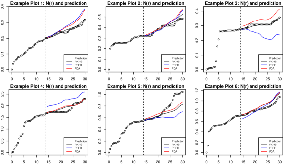
Figure 1: Observed (normalized) fundraising curves $\{N_{t}(r)\}$ (dots) of six representative campaigns and functional predictions (solid lines) given by RKHS, FDA and PFFR at $s=14$th day (dashed vertical line) based on the functional covariate $\{N_{t}(r),\,r\in[0,s]\}$.

1.1 Literature review

As mentioned in recent reviews, e.g. Wang et al. (2016) and Morris (2015), there are in general three types of functional linear regression models: 1) functional covariates and scalar or vector responses (e.g. Cardot et al., 2003; Cai and Hall, 2006; Hall and Horowitz, 2007; Yuan and Cai, 2010; Raskutti et al., 2012; Cai and Yuan, 2012; Jiang et al., 2014; Fan et al., 2015); 2) functional covariates and functional responses (e.g. Wu et al., 1998; Liang et al., 2003; Yao et al., 2005; Fan et al., 2014; Ivanescu et al., 2015; Sun et al., 2018) and 3) vector covariates and functional responses (e.g. Laird and Ware, 1982; Li and Hsing, 2010; Faraway, 1997; Wu and Chiang, 2000). Another closely related area is functional time series. For instance, functional autoregressive models also preserve the regression format. The literature on functional time series is also abundant, including van Delft et al. (2017), Aue et al. (2015), Bathia et al. (2010), Wang et al. (2020a) and many others.

Regarding the sampling scheme, to establish theoretical guarantees, it is often assumed in the literature that functions are fully observed, which is generally untrue in practice. To study the properties of functional regression under the more realistic scenario where functions are observed only on discrete sample points, one usually imposes certain smoothness conditions on the underlying functions. The errors introduced by the discretization of functions can therefore be controlled as a function of the smoothness level and $n$, the number of discretized observations available for each function. Some fundamental tools regarding this aspect were established in Mendelson (2002) and Bartlett et al. (2005), and were further applied to various regression analysis problems (e.g. Raskutti et al., 2012; Koltchinskii and Yuan, 2010; Cai and Yuan, 2012).

Regarding the statistical inference task, in the regression context, estimation and prediction are two indispensable pillars. In the functional regression literature, Valencia and Yuan (2013), Cai and Yuan (2011), Yuan and Cai (2010), Lin and Yuan (2006), Park et al. (2018), Fan et al. (2014), Fan et al. (2015), and Reimherr et al. (2019), among many others, have studied different aspects of the estimation problem. As for prediction, the existing literature includes Cai and Yuan (2012), Cai and Hall (2006), Ferraty and Vieu (2009), Sun et al. (2018), Reimherr et al. (2018) to name but a few.

In contrast to the aforementioned three paradigms of functional regression, in this paper, we study the functional linear regression problem in model (1) with functional responses and mixed predictors that consist of both functional and vector covariates. We assume the functions are only observed on discrete sample points and aim to derive optimal upper bounds on the excess prediction risk (see Definition 1). More detailed comparisons with existing literature are deferred till we present the main results in Section 3.

1.2 Main contributions

The main contributions of this paper are summarized as follows.

Firstly, to the best of our knowledge, the model we study in this paper, as defined in (1), is among the most flexible ones in the literature of functional linear regression. In terms of predictors, we allow for both functional and vector covariates. In terms of model dimensionality, we allow for the dimension $p$ of vector covariates to grow exponentially as the sample size $T$ diverges. In terms of function spaces, which will be elaborated later, we allow for the coefficients of the functional and vector covariates to be from different reproducing kernel Hilbert spaces (RKHS). In terms of dependence between the functional and vector covariates, we allow the correlation to be of order up to $O(1)$, which is a rather weak condition, especially considering that the vector covariates are of high dimensions. In terms of the sampling scheme, we allow for the functional covariate and response to be observed on (possibly different) discretized sample points. This general and unified framework imposes new challenges on both theory and optimization, as we elaborate in detail later.

Secondly, we develop new peeling techniques in our theoretical analysis, which is crucial and fundamental in dealing with the potentially exponentially growing vector covariate dimension. Existing asymptotic analysis techniques and results in the functional regression literature are insufficient to provide Lasso-type guarantees with the presence of high-dimensional covariates. See Remark 2 for more details.

Thirdly, we demonstrate an interesting phase transition phenomenon in terms of the smoothness of the functional covariate and the dimensionality of the vector covariate. To be specific, let $\mathfrak{s}$ be the sparsity of $\{\beta^{*}_{j}\}_{j=1}^{p}$, i.e. the number of non-zero univariate coefficient functions. Let $\delta_{T}$ be a quantity jointly determined by the complexities and the alignment of the two RKHS’s where the functional covariates $\{X_{t}\}_{t=1}^{T}$ and the bivariate coefficient function $A^{*}$ reside; see Theorem 2 for the detailed definition of $\delta_{T}$. We show that the excess prediction risk of our proposed estimator is upper bounded by

$$O_{\mathrm{p}}\left\{\mathfrak{s}\log(p\vee T)T^{-1}+\delta_{T}\right\}+\mbox{discretization error}.$$

• When $\delta_{T}\lesssim\mathfrak{s}\log(p\vee T)T^{-1}$, the excess risk is dominated by $\mathfrak{s}\log(p\vee T)T^{-1}$, which is the standard excess risk rate in the high-dimensional parametric statistics literature (e.g. Bühlmann and van de Geer, 2011). Therefore, the difficulty is dominated by estimating $\{\beta^{*}_{j}\}_{j=1}^{p}$, the $p$ univariate coefficient functions.

• When $\delta_{T}\gtrsim\mathfrak{s}\log(p\vee T)T^{-1}$, the excess risk is dominated by $\delta_{T}$, which suggests that the difficulty is dominated by estimating the bivariate coefficient function $A^{*}$. We show that in this regime, the optimal excess risk of model (1) is of order $\delta_{T}$. As a result, in this regime the difficulty is dominated by estimating the bivariate coefficient function $A^{*}$.

• We further develop matching lower bounds to justify that this phase transition between high-dimensional parametric rate and the non-parametric rate is indeed minimax optimal; see Section 3.3. To the best of our knowledge, this is the first time such phenomenon is observed in the functional regression literature.

Note that, this phase transition and its associated optimality are not with respect to the discretization error, i.e. $n$ - the minimum number of observations obtained for each function.

Lastly, we derive a representer theorem and further propose a novel optimization algorithm via iterative coordinate descent, which efficiently solves a sophisticated penalized least squares problem with the presence of both a ridge-type smoothing penalty and a group Lasso-type sparsity penalty.

The rest of the paper is organized as follows. In Section 2, we introduce relevant definitions and quantities. The main theoretical results are presented in Section 3. The optimization procedure is discussed in Section 4. Numerical experiments and real data applications are conducted in Section 5 to illustrate the favorable performance of the proposed estimator over existing approaches in the literature. Section 6 concludes with a discussion.

Notation

Let $\mathbb{N}_{*}$ denote the collection of positive integers. Let $a(n)$ and $b(n)$ be two quantities depending on $n$. We say that $a(n)\lesssim b(n)$ if there exists $n_{0}\in\mathbb{N}_{*}$ and an absolute constant $C>0$ such that for any $n\geq n_{0}$, $a(n)\leq Cb(n)$. We denote $a(n)\asymp b(n)$, if $a(n)\lesssim b(n)$ and $b(n)\lesssim a(n)$. For any function $g:[0,1]\to\mathbb{R}$, denote

$$\|g\|_{\mathcal{L}^{2}}=\sqrt{\int_{[0,1]}g^{2}(r)\,\mathrm{d}r}\quad\text{and}\quad\|g\|_{\infty}=\sup_{r\in[0,1]}|g(r)|.$$

For any $p\in\mathbb{N}_{*}$ and $a,b\in\mathbb{R}^{p}$, let $\langle a,b\rangle_{p}=\sum_{i=1}^{p}a_{i}b_{i}$.

Let $\mathcal{L}^{2}=\mathcal{L}^{2}([0,1])$ be the space of all square integrable functions with respect to the uniform distribution on $[0,1]$, i.e. $\mathcal{L}^{2}=\{f:[0,1]\to\mathbb{R},\,\|f\|_{\mathcal{L}^{2}}<\infty\}$. For any $\alpha>0$, let $W^{\alpha,2}$ be the Sobolev space of order $\alpha$. For a positive integer $\alpha$, we have

$$W^{\alpha,2}=\{f\in{\mathcal{L}^{2}}[0,1],\,f^{(\alpha-1)}\mbox{ is absolutely continuous}\mbox{ and }\|f^{(\alpha)}\|_{{\mathcal{L}^{2}}}<\infty\},$$

where $f^{(k)}$ is the $k$-th weak derivative of $f$, $k\in\mathbb{N}$. In this case the Sobolev norm of $f$ is defined as

$$\|f\|_{{W^{\alpha,2}}}^{2}=\|f\|_{\mathcal{L}^{2}}^{2}+\|f^{(\alpha)}\|_{\mathcal{L}^{2}}^{2}.$$

For non-integer valued $\alpha>0$, the Sobolev space $W^{\alpha,2}$ and the norm $\|\cdot\|_{{W^{\alpha,2}}}$ are also well-defined (e.g. see Brezis, 2010). Note that if $0<\alpha_{1}<\alpha_{2}$, then $W^{\alpha_{2},2}\subset W^{\alpha_{1},2}$.

2 Background

In this section, we provide some background on the fundamental tools used in this paper, with RKHS and compact linear operators studied in Section 2.1 and Section A.1, respectively.

2.1 Reproducing kernel Hilbert spaces (RKHS)

Consider a Hilbert space $\mathcal{H}\subset\mathcal{L}^{2}$ and its associated inner product $\langle\cdot,\cdot\rangle_{\mathcal{H}}$, under which $\mathcal{H}$ is complete. We assume that there exists a continuous symmetric nonnegative-definite kernel function $\mathbb{K}:[0,1]\times[0,1]\to\mathbb{R}_{+}$ such that the space $\mathcal{H}$ is an RKHS, in the sense that for each $r\in[0,1]$, the function $\mathbb{K}(\cdot,r)\in\mathcal{H}$ and $g(r)=\langle g(\cdot),\mathbb{K}(\cdot,r)\rangle_{\mathcal{H}}$, for all $g\in\mathcal{H}$. To emphasize this relationship, we write $\mathcal{H}(\mathbb{K})$ as an RKHS with $\mathbb{K}$ as the associated kernel. For any $\mathbb{K}$, we say it is a bounded kernel if $\sup_{r\in[0,1]}\mathbb{K}(r,r)<\infty$.

It follows from Mercer’s theorem (Mercer, 1909) that there exists an orthonormal basis of $\mathcal{L}^{2}$, $\{\phi_{k}\}_{k=1}^{\infty}\subset\mathcal{L}^{2}$, such that a non-negative definite kernel function $\mathbb{K}(\cdot,\cdot)$ has the representation $\mathbb{K}(s,r)=\sum_{k=1}^{\infty}\mu_{k}\phi_{k}(s)\phi_{k}(r),~{}s,r\in[0,1],$ where $\mu_{1}\geq\mu_{2}\geq\cdots\geq 0$ are the eigenvalues of $\mathbb{K}$ and $\{\phi_{k}\}_{k=1}^{\infty}$ are the corresponding eigenfunctions. In the rest of this paper, when there is no ambiguity, we drop the dependence of $\mu_{k}$’s and $\phi_{k}$’s on their associated kernel function $\mathbb{K}$ for ease of notation.

Note that any function $f\in\mathcal{H}(\mathbb{K})$ can be written as

$$f(r)=\sum_{k=1}^{\infty}\left\{\int_{[0,1]}f(r)\phi_{k}(r)\,\mathrm{d}r\right\}\phi_{k}(r)=\sum_{k=1}^{\infty}a_{k}\phi_{k}(r),\quad r\in[0,1],$$

and its RKHS norm is defined as $\|f\|_{{\mathcal{H}(\mathbb{K})}}=\sqrt{\sum_{k=1}^{\infty}{a_{k}^{2}}/{\mu_{k}}}.$ Thus, for the eigenfunctions, we have $\|\phi_{k}\|_{\mathcal{H}(\mathbb{K})}^{2}=\mu_{k}^{-1}$. Throughout this section, we further denote $\psi_{k}=\sqrt{\mu_{k}}\phi_{k}$ and note that $\|\psi_{k}\|_{\mathcal{H}(\mathbb{K})}=1$ for $k\in\mathbb{N}_{*}$.

Define the linear map $L_{\mathbb{K}}:{\mathcal{L}^{2}}\to{\mathcal{L}^{2}}$, associated with $\mathbb{K}$, as $L_{\mathbb{K}}(f)(\cdot)=\int_{[0,1]}\mathbb{K}(\cdot,r)f(r)\,\mathrm{d}r$. It holds that $L_{\mathbb{K}}(\phi_{k})=\mu_{k}\phi_{k}$, for $k\in\mathbb{N}_{*}$. Furthermore, define $L_{\mathbb{K}^{1/2}}:{\mathcal{L}^{2}}\to{\mathcal{H}(\mathbb{K})}$ such that $L_{\mathbb{K}^{1/2}}(\phi_{k})=\sqrt{\mu_{k}}\phi_{k}$, and define $L_{\mathbb{K}^{-1/2}}:{\mathcal{H}(\mathbb{K})}\to{\mathcal{L}^{2}}$ such that $L_{\mathbb{K}^{-1/2}}(\phi_{k})=\mu_{k}^{-1/2}\phi_{k}$, for $k\in\mathbb{N}_{*}$. For any two bivariate functions $R_{1}(\cdot,\cdot),R_{2}(\cdot,\cdot):[0,1]\times[0,1]\to\mathbb{R}$, define $R_{1}R_{2}(r,s)=\int_{[0,1]}R_{1}(r,u)R_{2}(u,s)\,\mathrm{d}u$, $r,s\in[0,1]$. It holds that $L_{R_{1}R_{2}}=L_{R_{1}}\circ L_{R_{2}}$, where $L_{R_{1}}\circ L_{R_{2}}$ represents the composition of $R_{1}$ and $R_{2}$, which is a linear map from ${\mathcal{L}^{2}}$ to ${\mathcal{L}^{2}}$ given that both $L_{R_{1}}$ and $L_{R_{2}}$ are linear maps from ${\mathcal{L}^{2}}$ to ${\mathcal{L}^{2}}$.

2.2 Bivariate functions and compact linear operators

To regulate the bivariate coefficient function $A^{*}$ in model (1), we consider a class of compact linear operators in ${\mathcal{H}(\mathbb{K})}$. Specifically, for any compact linear operator $A_{2}:{\mathcal{H}(\mathbb{K})}\to{\mathcal{H}(\mathbb{K})}$, denote

$$A_{2}[f,g]=\langle A_{2}[g],f\rangle_{\mathcal{H}(\mathbb{K})},\quad f,g\in{\mathcal{H}(\mathbb{K})}.$$

Note that $A_{2}[f,g]$ is well defined for any $f,g\in{\mathcal{H}(\mathbb{K})}$ due to the compactness of $A_{2}$. Let $\{\psi_{i}\}_{i=1}^{\infty}$ be the eigenbasis of ${\mathcal{H}(\mathbb{K})}$ and $a_{ij}=A_{2}[\psi_{i},\psi_{j}]=\langle A_{2}[\psi_{j}],\psi_{i}\rangle_{\mathcal{H}(\mathbb{K})}$, $i,j\in\mathbb{N}_{*}$. We thus have for any $f,g\in{\mathcal{H}(\mathbb{K})}$, it follows from Remark 4 in the appendix that

$$A_{2}[f,g] =\sum_{i,j=1}^{\infty}a_{ij}\langle f,\psi_{i}\rangle_{{\mathcal{H}(\mathbb{K})}}\langle g,\psi_{j}\rangle_{{\mathcal{H}(\mathbb{K})}}.$$ (2)

Note that via (2), we can define a bivariate function $A_{1}(r,s),~{}r,s\in[0,1]$, affiliated with the compact operator $A_{2}$. Specifically, plugging $f=\mathbb{K}(r,\cdot)$ and $g=\mathbb{K}(s,\cdot)$ into (2), we have that

$$A_{2}[\mathbb{K}(r,\cdot),\mathbb{K}(s,\cdot)]=\sum_{i,j=1}^{\infty}a_{ij}\langle\mathbb{K}(r,\cdot),\psi_{i}\rangle_{{\mathcal{H}(\mathbb{K})}}\langle\mathbb{K}(s,\cdot),\psi_{j}\rangle_{{\mathcal{H}(\mathbb{K})}}=\sum_{i,j=1}^{\infty}a_{ij}\psi_{i}(r)\psi_{j}(s)=A_{1}(r,s).$$

From the above set up, it holds that for all $v\in{\mathcal{H}(\mathbb{K})}$, we have

$$A_{2}[v](r)=\langle A_{1}(r,\cdot),v(\cdot)\rangle_{\mathcal{H}(\mathbb{K})},\quad r\in[0,1].$$

We have established an equivalence between a compact linear operator $A_{2}$ and its corresponding bivariate function $A_{1}(r,s)$, therefore any compact linear operator $A_{2}:{\mathcal{H}(\mathbb{K})}\to{\mathcal{H}(\mathbb{K})}$ can be viewed as a bivariate function $A_{1}:[0,1]\times[0,1]\to\mathbb{R}$.

To facilitate the later formulation of penalized convex optimization and the derivation of the representer theorem, we further focus on the Hilbert–Schmidt operator, which is an important subclass of compact operators. A compact operator $A_{2}$ is Hilbert–Schmidt if

$$\|A_{2}\|_{\mathrm{F}(\mathbb{K})}^{2}=\sum_{i,j=1}^{\infty}\langle A_{2}[\psi_{j}],\psi_{i}\rangle_{\mathcal{H}(\mathbb{K})}^{2}=\sum_{i,j=1}^{\infty}a_{ij}^{2}<\infty.$$ (3)

In the rest of this paper, for ease of presentation, we adopt some abuse of notation and refer to compact linear operators and the corresponding bivariate functions by the same notation $A$.

3 Main results

3.1 The constrained/penalized estimator and the representer theorem

Recall that in model (1), the response is the function $Y$, the covariates include the function $X$ and vector $Z$, and the unknown parameters are the bivariate coefficient function $A^{*}$ and univariate coefficient functions $\beta^{*}=\{\beta_{l}^{*}\}_{l=1}^{p}$. Given the observations $\{X_{t}(s_{i}),Z_{t},Y_{t}(r_{j})\}_{t=1,i=1,j=1}^{T,n_{1},n_{2}}$, our main task is to estimate $A^{*}$ and $\beta^{*}$.

Define the weight functions $w_{s}(i)=(n_{1}+1)(s_{i}-s_{i-1})$ for $1\leq i\leq n_{1}$ and $w_{r}(j)=(n_{2}+1)(r_{j}-r_{j-1})$ for $1\leq j\leq n_{2}$, where by convention we set $s_{0}=r_{0}=0$. In addition, for any $1\leq l\leq p$, define

$$\|\beta_{l}\|_{n_{2}}=\sqrt{\frac{1}{n_{2}}\sum_{j=1}^{n_{2}}w_{r}(j)\beta_{l}^{2}(r_{j})}.$$

We propose the following constrained/penalized least squares estimator

$$(\widehat{A},\widehat{\beta})=\operatorname*{arg\,min}_{\begin{subarray}{c}A\in\mathcal{C}_{A},\\ \beta=\{\beta_{l}\}_{l=1}^{p}\in\mathcal{C}_{\beta}\end{subarray}}\Bigg{[}\frac{1}{Tn_{2}}\sum_{t=1}^{T}\sum_{j=1}^{n_{2}}w_{r}(j)\left\{Y_{t}(r_{j})-\frac{1}{n_{1}}\sum_{i=1}^{n_{1}}w_{s}(i)A(r_{j},s_{i})X_{t}(s_{i})-\langle\beta(r_{j}),Z_{t}\rangle_{p}\right\}^{2}$$

$$\hskip 284.52756pt+\lambda\sum_{l=1}^{p}\|\beta_{l}\|_{n_{2}}\Bigg{]},$$ (4)

where $\lambda>0$ is a tuning parameter that controls the group Lasso penalty, $\mathcal{C}_{A}$ and $\mathcal{C}_{\beta}$ characterize the spaces of coefficient functions $A$ and $\beta$ respectively such that

$$\mathcal{C}_{A}=\{A:{\mathcal{H}(\mathbb{K})}\to{\mathcal{H}(\mathbb{K})},\,\|A\|_{{\mathrm{F}(\mathbb{K})}}^{2}\leq C_{A}\},\,\mathcal{C}_{\beta}=\Bigg{\{}\{\beta_{l}\}_{l=1}^{p}\subset{\mathcal{H}(\mathbb{K}_{\beta})}:\,\sum_{l=1}^{p}\|\beta_{l}\|_{{\mathcal{H}(\mathbb{K}_{\beta})}}\leq C_{\beta}\Bigg{\}}.$$ (5)

Here $C_{A},C_{\beta}>0$ are two absolute constants and $\|\cdot\|_{\mathrm{F}(\mathbb{K})}$ is defined in (3). Note that we allow the RKHS’s ${\mathcal{H}(\mathbb{K})}$ and ${\mathcal{H}(\mathbb{K}_{\beta})}$ to be generated by two different kernels $\mathbb{K}$ and $\mathbb{K}_{\beta}$. The detailed optimization scheme is deferred to Section 4.

The above optimization problem essentially constrains three tuning parameters. The tuning parameters $C_{A}$ and $C_{\beta}$ control the smoothness of the regression coefficient functions. These constrains are standard and ubiquitous in the functional data analysis and non-parametric statistical literature. The tuning parameter $\lambda$ controls the group Lasso penalty, which is used to encourage sparsity when the dimensionality $p$ diverges faster than the sample size $T$.

The optimization problem in (3.1) makes use of the weight functions ${w_{s}(i)}$ and ${w_{r}(j)}$, which are determined by the discrete sample points $\{s_{i}\}_{i=1}^{n_{1}}$ and $\{r_{j}\}_{j=1}^{n_{2}}$ respectively. This is designed to handle the scenario where the functional variables are observed on unevenly spaced sample points. Indeed, for evenly spaced sample points $\{s_{i}\}_{i=1}^{n_{1}}$ and $\{r_{j}\}_{j=1}^{n_{2}}$, we have that ${w_{s}(i)}={w_{r}(j)}=1$ for all $i,j$. We remark that it is well known that the integral of a regular function can be well approximated by its weighted sum evaluated at discrete sample points.

Note that (3.1) is an infinite dimensional optimization problem. Fortunately, Proposition 1 states that the estimator $(\widehat{A},\widehat{\beta})$ can in fact be written as linear combinations of their corresponding kernel functions evaluated at the discrete sample points $\{s_{i}\}_{i=1}^{n_{1}}$ and $\{r_{j}\}_{j=1}^{n_{2}}$.

Proposition 1

Denote $\mathbb{K}$ and $\mathbb{K}_{\beta}$ as the RKHS kernels of ${\mathcal{H}(\mathbb{K})}$ and ${\mathcal{H}(\mathbb{K}_{\beta})}$ respectively. There always exists a minimizer $(\widehat{A},\widehat{\beta})$ of (3.1) such that,

$$\widehat{A}(r,s)=\sum_{i=1}^{n_{1}}\sum_{j=1}^{n_{2}}\widehat{a}_{ij}\mathbb{K}(r,r_{j})\mathbb{K}(s,s_{i}),\quad(r,s)\in[0,1]\times[0,1],\,\{\widehat{a}_{ij}\}_{i,j=1}^{n_{1},n_{2}}\subset\mathbb{R},$$

and

$$\widehat{\beta}_{l}(r)=\sum_{j=1}^{n_{2}}\widehat{b}_{lj}\mathbb{K}_{\beta}(r_{j},r),\quad r\in[0,1],\,l\in\{1,\ldots,p\},\,\{\widehat{b}_{lj}\}_{l=1,j=1}^{p,n_{2}}\subset\mathbb{R}.$$

Proposition 1 is a generalization of the well-known representer theorem for RKHS (Wahba, 1990). Various versions of representer theorems are derived and used in the functional data analysis literature (e.g. Yuan and Cai, 2010).

3.2 Model assumptions

To establish the optimal theoretical guarantees for the estimator $(\widehat{A},\widehat{\beta})$, we impose some mild model assumptions, on the coefficient functions (1), functional and vector covariates (2) and sampling scheme (3).

Assumption 1 (Coefficient functions)

• The bivariate coefficient function $A^{*}$ belongs to $\mathcal{C}_{A}$ defined in (5), where ${\mathcal{H}(\mathbb{K})}$ is the RKHS associated with a bounded kernel $\mathbb{K}$ and $C_{A}>0$ is an absolute constant.

• The univariate coefficient functions $\{\beta^{*}_{l}\}_{l=1}^{p}$ belong to $\mathcal{C}_{\beta}$ defined in (5), where ${\mathcal{H}(\mathbb{K}_{\beta})}$ is the RKHS associated with a bounded kernel $\mathbb{K}_{\beta}$ and $C_{\beta}>0$ is an absolute constant.

  In addition, there exists a set $S\subset\{1,\ldots,p\}$ such that $\beta_{j}^{*}=0$ for all $j\in\{1,\ldots,p\}\setminus S$ and there exists a sufficiently large absolute constant $C_{\mathrm{snr}}>0$ such that

  $$T\geq C_{\mathrm{snr}}\mathfrak{s}\log(p\vee T),$$ (6)

  where $\mathfrak{s}=|S|$ denotes the cardinality of the set $S$.

1(a) requires the bivariate coefficient function $A^{*}$ to be a Hilbert–Schmidt operator mapping from ${\mathcal{H}(\mathbb{K})}$ to ${\mathcal{H}(\mathbb{K})}$. 1(b) imposes smoothness and sparsity conditions on the univariate coefficient functions $\{\beta_{l}^{*}\}_{l=1}^{p}$ to handle the potential high-dimensionality of the vector covariate. Note that we allow $\{\beta_{l}^{*}\}_{l=1}^{p}$ to be from a possibly different RKHS ${\mathcal{H}(\mathbb{K}_{\beta})}$ than ${\mathcal{H}(\mathbb{K})}$ and thus would allow users to choose kernels based on their practical needs.

Assumption 2 (Covariates)

• The functional noise $\{\epsilon_{t}\}_{t=1}^{T}$ is a collection of independent and identically distributed Gaussian processes such that $\mathbb{E}(\epsilon_{1}(r))=0$ and $\mathrm{Var}(\epsilon_{1}(r))<C_{\epsilon}$ for all $r\in[0,1]$. In addition, $\{\epsilon_{t}\}_{t=1}^{T}$ are independent of $\{X_{t},Z_{t}\}_{t=1}^{T}$.

• The functional covariate $\{X_{t}\}_{t=1}^{T}$ is a collection of independent and identically distributed centered Gaussian processes with covariance operator $\Sigma_{X}$ and $\mathbb{E}\big{(}\|X_{1}\|_{\mathcal{L}^{2}}^{2}\big{)}=C_{X}<\infty.$

• The vector covariate $\{Z_{t}\}_{t=1}^{T}\subset\mathbb{R}^{p}$ is a collection of independent and identically distributed Gaussian random vectors from $\mathcal{N}(0,\Sigma_{Z})$, where $\Sigma_{Z}\in\mathbb{R}^{p\times p}$ is a positive definite matrix such that

  $$c_{z}\|v\|^{2}_{2}\leq v^{\top}\Sigma_{Z}v\leq C_{z}\|v\|_{2}^{2},\quad v\in\mathbb{R}^{p},$$

  and $c_{z},C_{Z}>0$ are absolute constants.

• For any deterministic $f\in{\mathcal{H}(\mathbb{K})}$ and deterministic $v\in\mathbb{R}^{p}$, it holds that

  $$\mathbb{E}(\langle X_{1},f\rangle_{\mathcal{L}^{2}}Z^{\top}_{1}v)\leq\frac{3}{4}\sqrt{\mathbb{E}\{\langle X_{1},f\rangle_{\mathcal{L}^{2}}^{2}\}(v^{\top}\Sigma_{Z}v)}=\frac{3}{4}\sqrt{\Sigma_{X}[f,f](v^{\top}\Sigma_{Z}v)}.$$

2(a) and (b) state that both the functional noise $\{\epsilon_{t}\}_{t=1}^{T}$ and functional covariates $\{X_{t}\}_{t=1}^{T}$ are Gaussian processes. In fact, one could further relax them to be sub-Gaussian processes. Such assumptions are frequently used in high-dimensional functional literature such as Kneip et al. (2016) and Wang et al. (2020b). 2(d) allows that the functional and vector covariates to be correlated up to $3/4$, which means that the correlation, despite the functional and high-dimensional nature of the problem, can be of order $O(1)$. We do not claim the optimality of the constant $3/4$ but emphasize that this correlation cannot be equal to one, as detailed in Section A.2.

Assumptions 1 and 2 are sufficient for establishing theoretical guarantees if we require all functions (i.e. the functional responses and functional covariates) to be fully observed, which is typically not realistic in practice. To allow for discretized observations, we further introduce assumptions on the sampling scheme and on the smoothness of the functional covariates.

Assumption 3 (Sampling scheme)

• The discrete sample points $\{s_{i}\}_{i=1}^{n_{1}}$ and $\{r_{j}\}_{j=1}^{n_{2}}$ are collections of points with $0\leq s_{1}<s_{2}\ldots<s_{n_{1}}=1$ and $0\leq r_{1}<r_{2}\ldots<r_{n_{2}}=1$, and there exists an absolute constant $C_{d}$ such that

  $$s_{i}-s_{i-1}\leq\frac{C_{d}}{n_{1}}\quad\text{for all $1\leq i\leq n_{1}+1$ }\quad\text{and}\quad r_{j}-r_{j-1}\leq\frac{C_{d}}{n_{2}}\quad\text{for all $1\leq j\leq n_{2}+1$,}$$

  where by convention we set $s_{0}=r_{0}=0$.

• Suppose that ${\mathcal{H}(\mathbb{K})},{\mathcal{H}(\mathbb{K}_{\beta})}\subset W^{\alpha,2}$ for some $\alpha>1/2$. In addition, suppose that

  $$\mathbb{E}(\|X_{1}\|_{W^{\alpha,2}}^{2})<\infty.$$ (7)

3(a) allows the functional variables to be partially observed on discrete sample points. Importantly, 3(a) can accommodate both fixed and random sampling schemes. In particular, suppose the sample points are randomly generated from an unknown distribution on $[0,1]$ with a density function $\mu:\,[0,1]\to\mathbb{R}$ such that $\inf_{r\in[0,1]}\mu(r)>0$, we have 3(a) holds with high probability. We refer to Theorem 1 of Wang et al. (2014) for more details.

To handle the partially observed functional variables, 3(b) imposes the smoothness assumption that $X$, $A^{*}$ and $\{\beta^{*}_{j}\}_{j=1}^{p}$ can be enclosed by a common superset, the Sobolev space $W^{\alpha,2}$. In particular, (7) is a commonly used assumption for bivariate function estimation in the functional data analysis literature. See for example, Cai and Yuan (2010) and Wang et al. (2020b) and references therein. We emphasize that 3(b) indeed allows different smoothness levels for $X$, $A^{*}$ and $\{\beta^{*}_{j}\}_{j=1}^{p}$, and only requires that the least smooth space among $X$, $A^{*}$ and $\{\beta^{*}_{j}\}_{j=1}^{p}$ is covered by $W^{\alpha,2}$.

The condition (7) requires that the second moment of $\|X\|_{W^{\alpha,2}}$ is finite, which implies $X\in W^{\alpha,2}$ almost surely. Due to the fact that the functional covariates $\{X_{t}\}_{t=1}^{T}$ are partially observed, to derive finite-sample guarantees, we need to establish uniform control over the approximation error

$$\left|\int_{[0,1]}A(r,s)X_{t}(s)\,\mathrm{d}s-\frac{1}{n_{1}}\sum_{i=1}^{n_{1}}w_{s}(i)A(r,s_{i})X_{t}(s_{i})\right|\quad\text{for all }t\in\{1,\ldots,T\}.$$

This requires the realized sample paths $\{X_{t}\}_{t=1}^{T}$ to be regular. In particular, the second moment condition in (7) can be used to show that $\{\|X_{t}\|_{{W^{\alpha,2}}}\}_{t=1}^{T}$ are bounded with high probability, which implies $\{X_{t}\}_{t=1}^{T}$ are Hölder smooth with Hölder parameter $\alpha-1/2>0$ by the Morrey inequality (see Theorem 32 in Appendix E.1 for more details). In Example 1 in Section A, we further provide a concrete example to illustrate a sufficient condition for (7).

3.3 Theoretical guarantees

With the assumptions in hand, we establish theoretical guarantees and investigate the minimax optimality of the proposed estimator (3.1), via the lens of excess risk defined in Definition 1. The derivation of (8) is collected in Lemma 31.

Definition 1 (Excess prediction risk)

Let $(\widehat{A},\widehat{\beta})$ be any estimator of $(A^{*},\beta^{*})$ in model (1). The excess risk of $(\widehat{A},\widehat{\beta})$ is defined as

$$\mathcal{E}^{*}(\widehat{A},\widehat{\beta})= \mathbb{E}_{X^{*},Z^{*},Y^{*}}\left\{\int_{[0,1]}\left(Y^{*}(r)-\int_{[0,1]}\widehat{A}(r,s)X^{*}(s)\,\mathrm{d}s-\langle Z^{*},\widehat{\beta}(r)\rangle_{p}\right)^{2}\,\mathrm{d}r\right\}$$

$$-\mathbb{E}_{X^{*},Z^{*},Y^{*}}\left\{\int_{[0,1]}\left(Y^{*}(r)-\int_{[0,1]}A^{*}(r,s)X^{*}(s)\,\mathrm{d}s-\langle Z^{*},\beta^{*}(r)\rangle_{p}\right)^{2}\,\mathrm{d}r\right\}$$

$$= \mathbb{E}_{X^{*},Z^{*},Y^{*}}\left\{\int_{[0,1]}\left(\int_{[0,1]}\Delta_{A}(r,s)X^{*}(s)\,\mathrm{d}s+\langle Z^{*},\Delta_{\beta}(r)\rangle_{p}\right)^{2}\,\mathrm{d}r\right\},$$ (8)

where

• $\Delta_{A}(r,s)=\widehat{A}(r,s)-A^{*}(r,s)$ and $\Delta_{\beta}(r)=\widehat{\beta}(r)-\beta^{*}(r)$ for $s,r\in[0,1]$;

• the random objects $(X^{*},Z^{*},Y^{*})$ are independent from and identically distributed as the observed data generated from model (1).

Remark 1

Definition 1 is ubiquitously used to measure prediction accuracy in regression settings. Excess risks are usually considered to provide better quantification of prediction accuracy for the estimators of interest than the $\ell_{2}$ error bounds. Consequently, throughout our paper, we evaluate our proposed estimators using excess risks. We remark that as pointed out by Cai and Hall (2006) and Cai and Yuan (2012), much of the practical interest in the functional regression parameters is centered around applications for the purpose of prediction.

We are now ready to present our main results, which provide upper and lower bounds on the excess risk $\mathcal{E}^{*}(\widehat{A},\widehat{\beta})$ of the proposed estimator $(\widehat{A},\widehat{\beta})$ defined in (3.1). For notational simplicity, in the following, we assume without loss of generality that $n_{1}=n_{2}=n$. For $n_{1}\neq n_{2}$, all the statistical guarantees continue to hold by setting $n=\min\{n_{1},n_{2}\}$.

Upper bounds

Theorem 2

Under Assumptions 1, 2 and 3, suppose that the eigenvalues $\{\xi_{k}\}_{k=1}^{\infty}$ of the linear operator $L_{\mathbb{K}^{1/2}\Sigma_{X}\mathbb{K}^{1/2}}$ satisfy

$$\xi_{k}\asymp k^{-2r},$$ (9)

for some $r>1/2$. Let $(\widehat{A},\widehat{\beta})$ be any solution to (3.1) with the tuning parameter $\lambda=C_{\lambda}\sqrt{{\log(p\vee T)}{T}^{-1}}$ for some sufficiently large constant $C_{\lambda}$. For any $T\gtrsim\log(n)$, there exists an absolute constant $C>0$ such that with probability at least $1-8T^{-4}$, it holds that

$$\mathcal{E}^{*}(\widehat{A},\widehat{\beta})\leq C\log(T)\big{\{}\delta_{T}+\mathfrak{s}\log(p\vee T)T^{-1}+\zeta_{n}\big{\}},$$ (10)

where $\zeta_{n}=n^{-\alpha+1/2}$, $\mathfrak{s}$ is the sparsity parameter defined in 1(b) and $\delta_{T}=T^{-2r/(2r+1)}$.

Theorem 2 provides a high-probability upper bound on the excess risk $\mathcal{E}^{*}(\widehat{A},\widehat{\beta})$. The result is stated in a general way for any RKHS’s ${\mathcal{H}(\mathbb{K}_{\beta})}$ and ${\mathcal{H}(\mathbb{K})}$, provided that the spectrum of $L_{\mathbb{K}^{1/2}\Sigma_{X}\mathbb{K}^{1/2}}$ satisfies the polynomial decay rate in (9). There are three components in the upper bound in (10).

• The term $\delta_{T}$ is an upper bound on the error associated with the estimation of the bivariate coefficient function $A^{*}$ in the presence of functional noise. As formally stated in (9), $\delta_{T}$ is determined by the alignment between the kernel $\mathbb{K}$ of the RKHS that $A^{*}$ resides in and the covariance operator of $X$. This is the well-known nonparametric rate frequently seen in the functional regression literature, see e.g. Cai and Yuan (2012).

• The term $\mathfrak{s}\log(p)T^{-1}$ is an upper bound on the error associated with the estimation of the high-dimensional sparse univariate coefficient functions $\beta^{*}$ and is a parametric rate frequently seen in the high-dimensional linear regression settings (e.g. Bühlmann and van de Geer, 2011).

• The term $\zeta_{n}$ is an upper bound on the error due to the fact that the functional variables $\{X_{t},Y_{t}\}_{t=1}^{T}$ are only observed on discrete sample points. Recall model (1) consists of two components $\int_{[0,1]}A^{*}(\cdot,s)X_{t}(s)\,\mathrm{d}s$ and $\langle Z_{t},\beta^{*}(\cdot)\rangle$. The discretization errors are captured through $\zeta_{n}=n^{-\alpha+1/2}$, which only depends on the smoothness of ${W^{\alpha,2}}$ with $\alpha>1/2$.

We show later in Proposition 3 that, provided the sample points are dense enough, e.g. $n\gg T$, up to a logarithmic factor of $T$, this upper bound achieves minimax optimality. In Section L, we further provide numerical illustration for the nonparametric rate $\delta_{T}$ and the high-dimensional parametric rate $\mathfrak{s}\log(p\vee T)T^{-1}$ in Theorem 2.

Remark 2 (New peeling techniques)

To prove Theorem 2, we develop new peeling techniques to obtain new exponential tail bounds, which are crucial in dealing with the potentially exponentially growing dimension $p$.

Remark 3 (Phase transition)

For sufficiently many samples, i.e. large $n$, the upper bound in (10) implies that, there exists an absolute constant $C>0$ such that with large probability

$$\mathcal{E}^{*}(\widehat{A},\widehat{\beta})\leq C\log(T)\big{\{}\delta_{T}+\mathfrak{s}\log(p\vee T)T^{-1}\big{\}}.$$

This unveils a phase transition between the nonparametric regime and the high-dimensional parametric regime, governed by the eigen-decay of the linear operator $L_{\mathbb{K}^{1/2}\Sigma_{X}\mathbb{K}^{1/2}}$ and the sparsity of the univariate coefficient functions $\beta^{*}$. To be specific, if $\delta_{T}\gtrsim\mathfrak{s}\log(p\vee T)T^{-1}$, the high-probability upper bound on the excess risk is determined by the nonparametric rate $\delta_{T}$; otherwise, the high-dimensional parametric rate dominates.

Corollary 11 in Section B.2 further presents a formal theoretical guarantee which quantifies a discretized version of the excess risk defined in Definition 1 for the proposed estimators $(\widehat{A},\widehat{\beta})$. Due to the fact that the functional variables are only partially observed on discrete sample points, the discretized version of the excess risk can be more relevant in certain practical applications.

Lower bounds

In this section, we derive a matching lower bound on the excess risk $\mathcal{E}^{*}(\widehat{A},\widehat{\beta})$ and thus show that the upper bound provided in Theorem 2 is nearly minimax optimal in terms of the sample size $T$, the dimension $p$ and the sparsity parameter $\mathfrak{s}$, saving for a logarithmic factor. We establish the lower bound under the assumption that the functional variables $\{X_{t},Y_{t}\}_{t=1}^{T}$ are fully observed, which is equivalent to setting $n=\infty$. Thus, we do not claim optimality in terms of the number of sample points $n$ for the result in Theorem 2.

Proposition 3

Under Assumptions 1 and 2, suppose that the functional variables $\{X_{t},Y_{t}\}_{t=1}^{T}$ are fully observed and the eigenvalues $\{\xi_{k}\}_{k=1}^{\infty}$ of the linear operator $L_{\mathbb{K}^{1/2}\Sigma_{X}\mathbb{K}^{1/2}}$ satisfy $\xi_{k}\asymp k^{-2r}$, for some $r>1/2$. There exists a sufficiently small constant $c>0$ such that

$$\inf_{\widehat{A},\widehat{\beta}}\sup_{A^{*}\in\mathcal{C}_{A},\beta^{*}\in\mathcal{C}_{\beta}}\mathbb{E}\{\mathcal{E}^{*}(\widehat{A},\widehat{\beta})\}\geq c\{T^{-\frac{2r}{2r+1}}+\mathfrak{s}\log(p)T^{-1}\},$$

where the infimum is taken over all possible estimators of $A^{*}$ and $\beta^{*}$ based on the observations $\{X_{t},Z_{t},Y_{t}\}_{t=1}^{T}$.

3.4 Extension to functional responses with measurement errors

In this subsection, we consider the setting where the functional responses are corrupted with measurement errors. More precisely, let the functional response $Y_{t}(r)$ be generated as in (1). Assume we observe

$$y_{t,j}=Y_{t}(r_{j})+\mathfrak{E}_{t,j},\quad t\in\{1,\ldots,T\},\,j\in\{1,\ldots,n_{2}\},$$

where $\{\mathfrak{E}_{t,j}\}_{t=1,j=1}^{T,n_{2}}$ is a collection of independent and identically distributed sub-Gaussian measurement errors with mean zero and $\mathrm{Var}(\mathfrak{E}_{t,j})\leq C_{\mathfrak{E}}$.

Given the observations $\{X_{t}(s_{i}),Z_{t},y_{t,j}\}_{t=1,i=1,j=1}^{T,n_{1},n_{2}}$, consider

$$(\widehat{A},\widehat{\beta})=\operatorname*{arg\,min}_{\begin{subarray}{c}A\in\mathcal{C}_{A},\\ \beta=\{\beta_{l}\}_{l=1}^{p}\in\mathcal{C}_{\beta}\end{subarray}}\Bigg{[}\frac{1}{Tn_{2}}\sum_{t=1}^{T}\sum_{j=1}^{n_{2}}w_{r}(j)\left\{y_{t,j}-\frac{1}{n_{1}}\sum_{i=1}^{n_{1}}w_{s}(i)A(r_{j},s_{i})X_{t}(s_{i})-\langle\beta(r_{j}),Z_{t}\rangle_{p}\right\}^{2}$$

$$+\lambda\sum_{l=1}^{p}\|\beta_{l}\|_{n_{2}}\Bigg{]},$$ (11)

where $\mathcal{C}_{A}$ and $\mathcal{C}_{\beta}$ are defined in (5). Note that without the presence of measurement errors, i.e. $\mathfrak{E}_{t,j}=0$ for all $t$ and $j$, the estimator (3.4) is identical to (3.1) proposed for the setting with only functional noise. In what follows, we show that the excess risk of the estimator (3.4) also achieves the same convergence rate as that in Theorem 2.

Theorem 4

Suppose all the assumptions in Theorem 2 hold. Let $(\widehat{A},\widehat{\beta})$ be any solution to (3.4) with the tuning parameter $\lambda=C_{\lambda}\sqrt{{\log(p\vee T)}{T}^{-1}}$ for some sufficiently large constant $C_{\lambda}$. For any $T\gtrsim\log(n)$, there exists an absolute constant $C>0$ such that with probability at least $1-8T^{-4}$, it holds that

$$\mathcal{E}^{*}(\widehat{A},\widehat{\beta})\leq C\log(T)\big{\{}\delta_{T}+\mathfrak{s}\log(p\vee T)T^{-1}+\zeta_{n}\big{\}},$$ (12)

where $\zeta_{n}=n^{-\alpha+1/2}$, $\mathfrak{s}$ is the sparsity parameter defined in 1(b) and $\delta_{T}=T^{-2r/(2r+1)}$.

4 Optimization

In this section, we propose an efficient convex optimization algorithm for solving (3.1) given the observations $\{X_{t}(s_{i}),Z_{t},Y_{t}(r_{j})\}_{t=1,i=1,j=1}^{T,n_{1},n_{2}}$. We remark that identical optimization can be applied to (3.4). To ease presentation, in the following we assume without loss of generality that $\mathcal{H}(\mathbb{K})=\mathcal{H}(\mathbb{K}_{\beta})$, and thus $\mathbb{K}=\mathbb{K}_{\beta}$. The general case where $\mathbb{K}\neq\mathbb{K}_{\beta}$ can be handled in exactly the same way with more tedious notation. Section 4.1 formulates (3.1) as a convex optimization problem and Section 4.2 further proposes a novel iterative coordinate descent algorithm to efficiently solve the formulated convex optimization.

4.1 Formulation of the convex optimization

By the equivalence between constrained and penalized optimization (see e.g. Hastie et al., 2009), we can reformulate (3.1) into a penalized optimization such that

$$(\widehat{A},\widehat{\beta})=\operatorname*{arg\,min}_{A,\beta}\Bigg{[} \sum_{t=1}^{T}\sum_{j=1}^{n_{2}}w_{r}(j)\left\{Y_{t}(r_{j})-\frac{1}{n_{1}}\sum_{i=1}^{n_{1}}w_{s}(i)A(r_{j},s_{i})X_{t}(s_{i})-\langle\beta(r_{j}),Z_{t}\rangle_{p}\right\}^{2}$$

$$+\lambda_{1}\|A\|_{\mathrm{F}(\mathbb{K})}^{2}+\lambda_{2}\sum_{l=1}^{p}\|\beta_{l}\|_{\mathcal{H}(\mathbb{K})}+\lambda_{3}\sum_{l=1}^{p}\|\beta_{l}\|_{n_{2}}\Bigg{]},$$ (13)

where $\lambda_{1},\lambda_{2},\lambda_{3}>0$ denote tuning parameters. Note that for notational simplicity, we drop the factor ${1}/{(Tn_{2})}$ of the squared loss. In the following, we show that (4.1) can be solved via convex optimization.

We first define some necessary notation. For $t=1,\ldots,T$, denote the functional curves observed on discrete grids as

$$Y_{t}=[Y_{t}(r_{1}),Y_{t}(r_{2}),\cdots,Y_{t}(r_{n_{2}})]^{\top}\in\mathbb{R}^{n_{2}}\quad\mbox{and}\quad X_{t}=[X_{t}(s_{1}),X_{t}(s_{2}),\cdots,X_{t}(s_{n_{1}})]^{\top}\in\mathbb{R}^{n_{1}}.$$

Define $Y=[Y_{1},\cdots,Y_{T}]\in\mathbb{R}^{n_{2}\times T},\,X=[X_{1},\cdots,X_{T}]\in\mathbb{R}^{n_{1}\times T}$ and $Z=[Z_{1},\cdots,Z_{T}]\in\mathbb{R}^{p\times T}.$

For any $r,s\in[0,1]$, denote the RKHS kernels as

$$k_{1}(r)=[\mathbb{K}(r,r_{1}),\mathbb{K}(r,r_{2}),\cdots,\mathbb{K}(r,r_{n_{2}})]^{\top}\in\mathbb{R}^{n_{2}}\text{ and }k_{2}(s)=[\mathbb{K}(s,s_{1}),\mathbb{K}(s,s_{2}),\cdots,\mathbb{K}(s,s_{n_{1}})]^{\top}\in\mathbb{R}^{n_{1}}.$$

Denote $K_{1}=[k_{1}(r_{1}),k_{1}(r_{2}),\cdots,k_{1}(r_{n_{2}})]\in\mathbb{R}^{n_{2}\times n_{2}}$ and $K_{2}=[k_{2}(s_{1}),k_{2}(s_{2}),\cdots,k_{2}(s_{n_{1}})]\in\mathbb{R}^{n_{1}\times n_{1}}$. Note that $K_{1}=\langle k_{1}(r),k_{1}(r)\rangle_{\mathcal{H}(\mathbb{K})}$ and $K_{2}=\langle k_{2}(s),k_{2}(s)\rangle_{\mathcal{H}(\mathbb{K})}$, thus both are symmetric and positive definite matrices. Furthermore, denote $W_{S}=\text{diag}(w_{s}(1),w_{s}(2),\cdots,w_{s}(n_{1}))\in\mathbb{R}^{n_{1}\times n_{1}}$ and $W_{R}=\text{diag}(\sqrt{w_{r}(1)},\sqrt{w_{r}(2)},\cdots,\sqrt{w_{r}(n_{2})})\in\mathbb{R}^{n_{2}\times n_{2}}$ as the diagonal weight matrices. Define $Y^{*}=W_{R}Y$, $K_{1}^{*}=W_{R}K_{1}$ and $K_{2}^{*}=K_{2}W_{S}$.

By the representer theorem (Proposition 1), we have the minimizer of (4.1) taking the form

$${A}(r,s)=k_{1}(r)^{\top}Rk_{2}(s)\quad\text{and}\quad{\beta}_{l}(r)=k_{1}(r)^{\top}\mathbf{b}_{l},\quad l=1,\cdots,p,$$

where $R\in\mathbb{R}^{n_{2}\times n_{1}}$ is an $n_{2}\times n_{1}$ matrix and $\mathbf{b}_{l}=[b_{l1},b_{l2},\cdots,b_{ln_{2}}]^{\top}\in\mathbb{R}^{n_{2}}$ is an $n_{2}$-dimensional vector for $l=1,\cdots,p$. Denote $\beta(r)=[{\beta}_{1}(r),{\beta}_{2}(r),\cdots,{\beta}_{p}(r)]^{\top}=[\mathbf{b}_{1},\mathbf{b}_{2},\cdots,\mathbf{b}_{p}]^{\top}k_{1}(r)=B^{\top}k_{1}(r)$, where $B=[\mathbf{b}_{1},\mathbf{b}_{2},\cdots,\mathbf{b}_{p}]\in\mathbb{R}^{n_{2}\times p}$.

By straightforward algebra, we can rewrite the optimization problem in (4.1) as

$$\left\|Y^{*}-\frac{1}{n_{1}}K_{1}^{*}RK_{2}^{*}X-K_{1}^{*}BZ\right\|_{\mathrm{F}}^{2}+\lambda_{1}\mathrm{tr}(R^{\top}K_{1}RK_{2})+\lambda_{2}\sum_{l=1}^{p}\sqrt{\mathbf{b}_{l}^{\top}K_{1}\mathbf{b}_{l}}+\lambda_{3}\sum_{l=1}^{p}\sqrt{\frac{1}{n_{2}}\mathbf{b}_{l}^{\top}K_{1}^{*\top}K_{1}^{*}\mathbf{b}_{l}},$$ (14)

where $\|\cdot\|_{\mathrm{F}}$ and $\text{tr}(\cdot)$ are the Frobenius norm and trace of a matrix. We refer to Section F.1 for the detailed derivation.

It is easy to see that (14) is a convex function of $R$ and $B$. Note that the first two terms of (14) are quadratic functions and can be handled easily, while the main difficulty of the optimization lies in the group Lasso-type penalty $\lambda_{2}\sum_{l=1}^{p}\sqrt{\mathbf{b}_{l}^{\top}K_{1}\mathbf{b}_{l}}+\lambda_{3}\sum_{l=1}^{p}\sqrt{\mathbf{b}_{l}^{\top}K_{1}^{*\top}K_{1}^{*}\mathbf{b}_{l}/n_{2}}$.

4.2 Iterative coordinate descent

In this section, we propose an efficient iterative coordinate descent algorithm which solves (14) by iterating between the optimization of $R$ and $B$.

Optimization of $R$ (i.e. the bivariate coefficient function $A$): Given a fixed $B=\left[\mathbf{b}_{1},\mathbf{b}_{2},\cdots,\mathbf{b}_{p}\right]$, denote $\widetilde{Y}=Y^{*}-K_{1}^{*}BZ\in\mathbb{R}^{n_{2}\times T}$. We have that (14) reduces to a function of $R$ that

$$\|\widetilde{Y}-n_{1}^{-1}K_{1}^{*}RK_{2}^{*}X\|_{\mathrm{F}}^{2}+\lambda_{1}\mathrm{tr}(R^{\top}K_{1}RK_{2}).$$ (15)

Define $E=K_{1}^{1/2}RK_{2}^{1/2}\in\mathbb{R}^{n_{2}\times n_{1}}$ and $\mathbf{e}=\mathrm{vec}(E).$ Denote $\widetilde{\mathbf{y}}=\mathrm{vec}(\widetilde{Y})=[\widetilde{Y}_{1}^{\top},\widetilde{Y}_{2}^{\top},\cdots,\widetilde{Y}_{T}^{\top}]^{\top}$ and denote $S_{1}=n_{1}^{-1}(X^{\top}W_{S}K_{2}^{1/2})\otimes(W_{R}K_{1}^{1/2})\in\mathbb{R}^{Tn_{1}\times n_{1}n_{2}}$. We can rewrite (15) as

$$\|\widetilde{\mathbf{y}}-S_{1}{\mathbf{e}}\|_{2}^{2}+\lambda_{1}\|{\mathbf{e}}\|_{2}^{2},$$ (16)

which can be seen as a classical ridge regression with a structured design matrix $S_{1}$. This ridge regression has a closed-form solution and can be solved efficiently by exploiting the Kronecker structure of $S_{1}$, see Section F.2 for more details. Thus, given $B$, $R$ can be updated efficiently.

Optimization of $B$ (i.e. the univariate coefficient functions $\beta$): Given a fixed $R$, with some abuse of notation, denote $\widetilde{Y}=Y^{*}-n_{1}^{-1}K_{1}^{*}RK_{2}^{*}X\in\mathbb{R}^{n_{2}\times T}$. For $l=1,\ldots,p$, define $\mathbf{h}_{l}=K_{1}^{*}\mathbf{b}_{l}\in\mathbb{R}^{n_{2}}$ and $H=K_{1}^{*}B=[\mathbf{h}_{1},\mathbf{h}_{2},\cdots,\mathbf{h}_{p}]\in\mathbb{R}^{n_{2}\times p}$. Further define $K_{3}=(K_{1}^{*})^{-1}K_{1}(K_{1}^{*})^{-1}$. We have that (14) reduces to a function of $H$ (and thus $B$), i.e.

$$\left\|\widetilde{Y}-HZ\right\|_{\mathrm{F}}^{2}+\lambda_{2}\sum_{l=1}^{p}\sqrt{\mathbf{h}_{l}^{\top}K_{3}\mathbf{h}_{l}}+\lambda_{3}\sum_{l=1}^{p}\sqrt{\frac{1}{n_{2}}\mathbf{h}_{l}^{\top}\mathbf{h}_{l}}$$

$$= \sum_{t=1}^{T}\left\|\widetilde{Y}_{t}-\sum_{l=1}^{p}Z_{tl}\mathbf{h}_{l}\right\|^{2}_{2}+\lambda_{2}\sum_{l=1}^{p}\sqrt{\mathbf{h}_{l}^{\top}K_{3}\mathbf{h}_{l}}+\frac{\lambda_{3}}{\sqrt{n_{2}}}\sum_{l=1}^{p}\|\mathbf{h}_{l}\|_{2},$$ (17)

which can be seen as a linear regression with two group penalties: a weighted group Lasso penalty and a standard group Lasso penalty. We solve the optimization of (4.2) by performing coordinate descent on $\mathbf{h}_{l},l=1,2\cdots,p$. See Friedman et al. (2010) for a similar strategy used to solve the sparse group Lasso problem for a linear regression with both a Lasso and a group Lasso penalty.

Specifically, for each $l=1,2,\cdots,p$, the Karush–Kuhn–Tucker condition for $\mathbf{h}_{l}$ is

$$-2\sum_{t=1}^{T}Z_{tl}\left(\widetilde{Y}_{t}-\sum_{l=1}^{p}Z_{tl}\mathbf{h}_{l}\right)+\lambda_{2}K_{4}\mathbf{s}_{l}^{(1)}+\frac{\lambda_{3}}{\sqrt{n_{2}}}\mathbf{s}_{l}^{(2)}=0.$$

Define $K_{4}$ as the root of $K_{3},$ i.e. $K_{4}K_{4}=K_{3}.$ We have that $K_{4}\mathbf{s}_{l}^{(1)}$ and $\mathbf{s}_{l}^{(2)}$ are the subgradients of $\sqrt{\mathbf{h}_{l}^{\top}K_{3}\mathbf{h}_{l}}$ and $\|\mathbf{h}_{l}\|_{2}$ respectively, such that

$$\mathbf{s}_{l}^{(1)}=\begin{cases}{K_{4}\mathbf{h}_{l}}/{\|K_{4}\mathbf{h}_{l}\|_{2}},&\mathbf{h}_{l}\neq 0,\\ \text{a vector with }\|\mathbf{s}_{l}^{(1)}\|_{2}\leq 1,&\mathbf{h}_{l}=0,\end{cases}~{}\text{ and }~{}\mathbf{s}_{l}^{(2)}=\begin{cases}{\mathbf{h}_{l}}/{\|\mathbf{h}_{l}\|_{2}},&\mathbf{h}_{l}\neq 0,\\ \text{a vector with }\|\mathbf{s}_{l}^{(2)}\|_{2}\leq 1,&\mathbf{h}_{l}=0.\end{cases}$$

Define $\widetilde{Y}_{t}^{l}=\widetilde{Y}_{t}-\sum_{j\neq l}Z_{tj}\mathbf{h}_{j}$. Thus, given $\{\mathbf{h}_{j},j\neq l\}$, we have that $\mathbf{h}_{l}=0$ is the optimal solution if there exist two vectors $\mathbf{s}_{l}^{(1)}$ and $\mathbf{s}_{l}^{(2)}$ with $\|\mathbf{s}_{l}^{(1)}\|_{2}\leq 1$ and $\|\mathbf{s}_{l}^{(2)}\|_{2}\leq 1$, and

$$\mathbf{s}_{l}^{(1)}=\frac{1}{\lambda_{2}}K_{4}^{-1}\left(2\sum_{t=1}^{T}Z_{tl}\widetilde{Y}_{t}^{l}-\frac{\lambda_{3}}{\sqrt{n}}\mathbf{s}_{l}^{(2)}\right).$$

This is equivalent to checking

$$\min_{\|\mathbf{s}\|_{2}\leq 1}\left\|2\sum_{t=1}^{T}Z_{tl}\widetilde{Y}_{t}^{l}-\frac{\lambda_{3}}{\sqrt{n}}\mathbf{s}\right\|_{2}\leq 1,$$

which is a standard constrained optimization problem and can be solved efficiently.

Otherwise, $\mathbf{h}_{l}\neq 0$ and to update $\mathbf{h}_{l}$, we need to optimize

$$\sum_{t=1}^{T}\|\widetilde{Y}_{t}^{l}-Z_{tl}\mathbf{h}_{l}\|^{2}_{2}+\lambda_{2}\sqrt{\mathbf{h}_{l}^{\top}K_{3}\mathbf{h}_{l}}+\frac{\lambda_{3}}{\sqrt{n_{2}}}\|\mathbf{h}_{l}\|_{2}.$$ (18)

We again solve this optimization by performing coordinate descent on $\mathbf{h}_{lk},k=1,2,\cdots,n_{2}$, where for each $k$, given $\{\mathbf{h}_{lj},j\neq k\}$, we can update $\mathbf{h}_{lk}$ by solving a simple one-dimensional optimization

$$\min\left\{\sum_{t=1}^{T}(\widetilde{Y}_{tk}^{l}-Z_{tl}\mathbf{h}_{lk})^{2}+\lambda_{2}\sqrt{K_{3,kk}\mathbf{h}_{lk}^{2}+2\mathbf{h}_{lk}\sum_{j\neq k}K_{3,kj}\mathbf{h}_{lj}+\sum_{i,j\neq k}\mathbf{h}_{li}K_{3,ij}\mathbf{h}_{lj}}+\frac{\lambda_{3}}{\sqrt{n_{2}}}\sqrt{\mathbf{h}_{lk}^{2}+\sum_{j\neq k}\mathbf{h}_{lj}^{2}}\right\}.$$ (19)

Thus, given $R$, $B$ can also be updated efficiently.

The iterative coordinate descent algorithm: Algorithm 1 formalizes the above discussion and outlines the proposed iterative coordinate descent algorithm. The convergence of coordinate descent for convex optimization is guaranteed under mild conditions, see e.g. Wright (2015). Empirically, the proposed algorithm is found to be efficient and stable, and typically reaches a reasonable convergence tolerance within a few iterations.

Algorithm 1 Iterative coordinate descent

1:input: Observations $\{X_{t}(s_{i}),Z_{t},Y_{t}(r_{j})\}_{t=1,i=1,j=1}^{T,n_{1},n_{2}}$, tuning parameters $(\lambda_{1},\lambda_{2},\lambda_{3})$, the maximum iteration $L_{max}$ and tolerance $\epsilon$.

2:initialization: $L=1,B_{0}=R_{0}=0.$

3:repeat$\triangleright$ First level block coordinate descent

4:     Given $B=B_{L-1}$, update $R_{L}$ via the ridge regression formulation (16).

5:     Given $R=R_{L}$, set $\widetilde{Y}=Y^{*}-{1}/{n_{1}}K_{1}^{*}RK_{2}^{*}X$ and initialize $H=K_{1}^{*}B_{L-1}$.

6:     repeat$\triangleright$ Second level coordinate descent

7:         for $l=1,2,\cdots,p$ do

8:              Given $\{\mathbf{h}_{j},j\neq l\}$, set $\widetilde{Y}_{t}^{l}=\widetilde{Y}_{t}-\sum_{j\neq l}Z_{tj}\mathbf{h}_{j},$ for $t=1,\cdots,T$.

9:              if $\min_{\|\mathbf{s}\|_{2}\leq 1}\left\|2\sum_{t=1}^{T}Z_{tl}\widetilde{Y}_{t}^{l}-\frac{\lambda_{3}}{\sqrt{n}}\mathbf{s}\right\|_{2}\leq 1$ then

10:                  Update $\mathbf{h}_{l}=0$.

11:              else

12:                  repeat$\triangleright$ Third level coordinate descent

13:                       for $k=1,2,\cdots,n_{2}$ do

14:                           Given $\{\mathbf{h}_{lj},j\neq k\}$, update $\mathbf{h}_{lk}$ via the one-dimensional optimization (19).

15:                       end for

16:                  until Decrease of function value (18) $<\epsilon$.

17:              end if

18:         end for

19:     until Decrease of function value (4.2) $<\epsilon$.

20:     Update $B_{L}=K_{1}^{*-1}H$ and set $L\leftarrow L+1$.

21:until Decrease of function value (14) $<\epsilon$ or $L\geq L_{max}$.

22:output: $\widehat{R}=R_{L}$ and $\widehat{B}=B_{L}$.

5 Numerical results

In this section, we conduct extensive numerical experiments to investigate the performance of the proposed RKHS-based penalized estimator (hereafter RKHS) for the functional linear regression with mixed predictors. Sections 5.1-5.3 compare RKHS with popular methods in the literature via simulation studies. Section 5.4 presents a real data application on crowdfunding prediction to further illustrate the potential utility of the proposed method. The implementations of our numerical experiments can be found at https://github.com/darenwang/functional_regression.

5.1 Simulation settings

Data generating process: We simulate data from the functional linear regression model

$$Y_{t}(r)=\int_{[0,1]}A^{*}(r,s)X_{t}(s)\,\mathrm{d}s+\sum_{j=1}^{p}\beta^{*}_{j}(r)Z_{tj}+\epsilon_{t}(r),\quad r\in[0,1],$$ (20)

for $t=1,2,\ldots,T.$ Note that for $p=0$, (20) reduces to the classical function-on-function regression.

We generate the functional covariate $\{X_{t}\}$ and the functional noise $\{\epsilon_{t}\}$ from a $q$-dimensional subspace spanned by basis functions $\{u_{i}(s)\}_{i=1}^{q}$, where $\{u_{i}(s)\}_{i=1}^{q}$ consists of orthonormal basis of $\mathcal{L}^{2}[0,1]$. Following Yuan and Cai (2010), we set $u_{i}(s)=1$ if $i=1$ and $u_{i}(s)=\sqrt{2}\cos((i-1)\pi s)$ for $i=2,\ldots,q$. Thus, we have $X_{t}(r)=\sum_{i=1}^{q}x_{ti}u_{i}(r)$ and $\epsilon_{t}(r)=\sum_{i=1}^{q}e_{ti}u_{i}(r)$. For $x_{t}=(x_{t1},\ldots,x_{tq})^{\top}$, we simulate $x_{ti}\stackrel{{\scriptstyle\mbox{i.i.d.}}}{{\sim}}\text{Unif}[-1/i,1/i]$, $i=1,\ldots,q$. For $e_{t}=(e_{t1},\ldots,e_{tq})^{\top}$, we simulate $e_{ti}\stackrel{{\scriptstyle\mbox{i.i.d.}}}{{\sim}}\text{Unif}[-0.2/i,0.2/i]$, $i=1,\ldots,q$. For the vector covariate $\{Z_{tj}\}$, we simulate $Z_{tj}\stackrel{{\scriptstyle\mbox{i.i.d.}}}{{\sim}}\text{Unif}[-1/\sqrt{3},1/\sqrt{3}]$, $j=1,\ldots,p$.

For the coefficient functions $A^{*}(r,s)$ and $\{\beta^{*}_{j}(r)\}_{j=1}^{p}$, we consider Scenarios A and B.

• Scenario A (Exponential): We set $A^{*}(r,s)=\kappa\sqrt{3}e^{-(r+s)}$, $\beta^{*}_{1}(r)=\kappa\sqrt{3}e^{-r}$ and $\beta_{j}^{*}(r)\equiv 0$, $j=2,\ldots,p$.

• Scenario B (Random): We set $A^{*}(r,s)=\kappa\sum_{i,j=1}^{q}\lambda_{ij}u_{i}(r)u_{j}(s)$, $\beta^{*}_{1}(r)=\kappa\sum_{i=1}^{q}b_{i}u_{i}(r)$ and $\beta^{*}_{j}(r)\equiv 0$, $j=2,\ldots,p$. Define matrix $\Lambda=(\lambda_{ij})$ and $b=(b_{1},\ldots,b_{q})^{\top}.$ We simulate $\lambda_{ij}\stackrel{{\scriptstyle\mbox{i.i.d.}}}{{\sim}}\mathcal{N}(0,1)$ and rescale $\Lambda$ such that its spectral norm $\|\Lambda\|_{\mathrm{op}}=1.$ For $b$, we simulate $b_{i}\stackrel{{\scriptstyle\mbox{i.i.d.}}}{{\sim}}\mathcal{N}(0,1)$ and rescale $b$ such that $\|b\|_{2}=1.$

Note that $(A^{*},\beta^{*})$ in Scenario B is more complex than that in Scenario A, especially when $q$ is large, while for Scenario A, its complexity is insensitive to $q$. The parameter $\kappa$ is later used to control the signal-to-noise ratio (SNR). Here, we define the SNR for $A^{*}(r,s)$ as

$$\sqrt{\mathbb{E}\int_{[0,1]}\bigg{[}\int_{[0,1]}A^{*}(r,s)X_{t}(s)\,\mathrm{d}s\bigg{]}^{2}dr}\bigg{/}\sqrt{\mathbb{E}\int_{[0,1]}\epsilon_{t}(r)^{2}\,\mathrm{d}r},$$

which roughly equals to 1, 2 and 4 as we vary $\kappa=0.5,1,2.$ Similarly, we define SNR for $\beta^{*}$ (note that only $\beta_{1}^{*}$ is a non-zero function) as

$$\sqrt{\mathbb{E}\int_{[0,1]}\bigg{[}\beta_{1}^{*}(r)Z_{t1}\bigg{]}^{2}\,\mathrm{d}r}\bigg{/}\sqrt{\mathbb{E}\int_{[0,1]}\epsilon_{t}(r)^{2}\,\mathrm{d}r},$$

which also roughly equals to 1, 2 and 4 as we vary $\kappa=0.5,1,2.$

For simplicity, we set the discrete sample points $\{r_{j}\}_{j=1}^{n_{2}}$ for $Y_{t}$ and $\{s_{i}\}_{i=1}^{n_{1}}$ for $X_{t}$ to be evenly spaced grids on $[0,1]$ with the same number of grids $n=n_{1}=n_{2}$. The simulation result for random sample points where $\{r_{j}\}_{j=1}^{n_{2}}$ and $\{s_{i}\}_{i=1}^{n_{1}}$ are generated independently via the uniform distribution on [0,1] is similar and thus omitted.

Evaluation criteria: We evaluate the performance of the estimator by its excess risk. Specifically, given the sample size $(n,T)$, we simulate observations $\{X_{t}(s_{i}),Z_{t},Y_{t}(r_{j})\}_{t=1,i=1,j=1}^{T+0.5T,n,n}$, which are then split into the training data $\{X_{t}(s_{i}),Z_{t},Y_{t}(r_{j})\}_{t=1,i=1,j=1}^{T,n,n}$ for constructing the estimator $(\widehat{A},\widehat{\beta})$ and the test data $\{X_{t}(s_{i}),Z_{t},Y_{t}(r_{j})\}_{t=T+1,i=1,j=1}^{T+0.5T,n,n}$ for the evaluation of the excess risk. Based on $(\widehat{A},\widehat{\beta})$ and the predictors $\{X_{t}(s_{i}),Z_{t}\}_{t=T+1,i=1}^{T+0.5T,n}$, we generate the prediction $\{\widehat{Y}_{t}(r)\}_{t=T+1}^{T+0.5T}$ and define

$$\text{RMISE}(\widehat{A},\widehat{\beta})=\sqrt{\frac{1}{0.5T}\sum_{t=T+1}^{T+0.5T}\int_{[0,1]}\left(Y_{t}^{\text{oracle}}(r)-\widehat{Y}_{t}(r)\right)^{2}\,\mathrm{d}r},$$ (21)

$$\text{nRMISE}(\widehat{A},\widehat{\beta})=\sqrt{\frac{\frac{1}{0.5T}\sum_{t=T+1}^{T+0.5T}\int_{[0,1]}\left(Y_{t}^{\text{oracle}}(r)-\widehat{Y}_{t}(r)\right)^{2}\,\mathrm{d}r}{\frac{1}{0.5T}\sum_{t=T+1}^{T+0.5T}\int_{[0,1]}\left(Y_{t}^{\text{oracle}}(r)-0\right)^{2}\,\mathrm{d}r}},$$ (22)

where $Y_{t}^{\text{oracle}}(r)=\int_{[0,1]}A(r,s)X_{t}(s)\,\mathrm{d}s+\beta_{1}(r)Z_{t1}$ is the oracle prediction of $Y_{t}(r)$. Note that nRMISE is a normalized RMISE, which can be viewed as a percentage error and thus is easy to assess and interpret. Smaller RMISE and nRMISE indicate a better recovery of the signal.

Simulation settings: We consider three simulation settings for $(n,T,q)$ where $(n,T,q)\in\{(5,50,5),(20,100,20),(40,200,50)\}.$ For each setting, we vary $\kappa\in\{0.5,1,2\}$, which roughly corresponds to $\text{SNR}\in\{1,2,4\}.$ As for the number of scalar predictors $p$, Section 5.2 considers the classical function-on-function regression, which is a special case of (20) with $p=0$ and Section 5.3 considers functional regression with mixed predictors and sets $p=3,10,50,100,200$. For each setting, we conduct 500 experiments.

Implementation details of the RKHS estimator: We set $\mathbb{K}=\mathbb{K}_{\beta}$ and use the rescaled Bernoulli polynomial as the reproducing kernel such that

$\mathbb{K}(x,y)=1+k_{1}(x)k_{1}(y)+k_{2}(x)k_{2}(y)-k_{4}(x-y),$

where $k_{1}(x)=x-0.5$, $k_{2}(x)=2^{-1}\{k_{1}^{2}(x)-1/12\}$, $k_{4}(x)=1/24\{k_{1}^{4}(x)-k_{1}^{2}(x)/2+7/240\}$, $x\in[0,1]$, and $k_{4}(x-y)=k_{4}(|x-y|)$, $x,y\in[0,1]$. Such $\mathbb{K}$ is the reproducing kernel for $W^{2,2}$. See Chapter 2.3.3 of Gu (2013) for more details. In Algorithm 1, we set the tolerance parameter $\epsilon=10^{-8}$ and the maximum iterations $L_{\max}=10^{4}.$ A standard 5-fold cross-validation (CV) on the training data is used to select the tuning parameters $(\lambda_{1},\lambda_{2},\lambda_{3})$. Note that for $p=0$, we explicitly set $\beta\equiv 0$ in the penalized optimization $\eqref{eq:approx A beta_penalized}$, which reduces to the structured ridge regression in (16) and can be solved efficiently with a closed-form solution as detailed in Section 4.2.

5.2 Function-on-function regression

In this subsection, we set $p=0$ and compare the proposed RKHS estimator with two popular methods in the literature for function-on-function regression.

The first competitor (Ramsay and Silverman, 2005) estimates the coefficient function $A(r,s)$ based on a penalized B-spline basis function expansion. We denote this approach as FDA and it is implemented via the R package fda.usc (fregre.basis.fr function). The second competitor (Ivanescu et al., 2015) is the penalized flexible functional regression (PFFR) in and is implemented via the R package refund (pffr function). Unlike our proposed RKHS method, neither FDA or PFFR has optimal theoretical guarantees.

Both FDA and PFFR are based on penalized basis function expansions and require a hyper-parameter $N_{b}$, which is the number of basis. Intuitively, the choice of $N_{b}$ is related to the complexity of $A^{*}(r,s)$, which is unknown in practice. In the literature, it is recommended to set $N_{b}$ at a large number to guard against the underfitting of $A^{*}(r,s)$. On the other hand, a larger $N_{b}$ can potentially incur higher estimation variance and will also increase the computational cost. For a fair comparison, for both FDA and PFFR we set $N_{b}=20$, which is sufficient to accommodate the model complexity across all simulation settings except for Scenario B with $q=50$. See more discussions later. We use a standard 5-fold CV to select the tuning parameter $\lambda_{1}$ of RKHS and the roughness penalty of FDA from the range $10^{(-15:0.5:2)}$. PFFR uses a restricted maximum likelihood (REML) approach to automatically select the roughness penalty.

Besides the penalized method based on basis function expansions (i.e. FDA and PFFR), another popular method for function-on-function regression in the literature is based on functional PCA (i.e. the Karhunen–Loéve expansion, FPCA), see for example Yao et al. (2005). However, FPCA does not seem to perform competitively in our simulation and real data analysis, see similar observations in Cai and Yuan (2012) and Sun et al. (2018). For completeness, we report the performance of FPCA in Section H and Section K.

Numerical results: For each method, Table 1 reports its average nRMISE (nRMISE_avg) across 500 experiments under all simulation settings. For each simulation setting, we further report R_avg, which is the percentage improvement of excess risk given by RKHS defined as

R_avg=[$\min\{$nRMISE_avg(FDA), nRMISE_avg(PFFR)$\}$ / nRMISE_avg(RKHS$)-1]\times 100\%$.

In addition, we report R_w, which is the percentage of experiments (among 500 experiments) where RKHS gives the lowest RMISE. We further give the boxplot of RMISE in Figure 2 under $\kappa=1$. The boxplots of RMISE under $\kappa\in\{0.5,2\}$ can be found in Section G.

As can be seen, RKHS in general delivers the best performance across almost all simulation settings. For all methods, the estimation performance improves with a larger SNR (reflected in $\kappa$). Since the complexity of Scenario A is insensitive to $q$, the performance of all methods improve as $(n,T)$ increases under Scenario A. However, this is not the case for Scenario B, as a larger $q$ increases the estimation difficulty. Compared to Scenario A, the excess risk RMISE of Scenario B is larger, especially for $q\in\{20,50\}$, due to the more complex nature of the operator $A^{*}.$ In general, the improvement of RKHS is more notable under high model complexity and SNR.

Note that for Scenario B with $q=50$, both FDA and PFFR incur significantly higher excess risks due to the underfitting bias caused by the insufficient basis dimension $N_{b}$, indicating the potential sensitivity of the penalized basis function approaches to the hyper-parameter. In comparison, RKHS automatically adapts to different levels of model complexity. In Section J, we further conduct the same simulation but with a larger number of basis dimension $N_{b}=50$ for FDA and $N_{b}=30$ for PFFR. For Scenario A, where the bivariate function $A^{*}(r,s)$ is a simple exponential function, FDA and PFFR give essentially the same performance, while for Scenario B with $q=50$, FDA and PFFR give much improved performance due to lower underfitting bias, though still having a notable performance gap compared to RKHS. In addition, note that a larger $N_{b}$ can significantly increase the computational cost of the penalized basis function approaches. We refer to Section J for more details.

In addition, Section I collects the results of the same simulation but with the observed functional responses $Y_{t}(r)$ being additionally corrupted with measurement errors, i.e. the scenario discussed in Section 3.4 (see Theorem 4). It is seen that the performance of RKHS only worsens slightly with the additional measurement errors, providing numerical support for Theorem 4 that measurement errors do not affect the convergence rate of RKHS.

	Scenario A: $n=5,T=50,q=5$					Scenario B: $n=5,T=50,q=5$
$\kappa$	RKHS	FDA	PFFR	Ravg(%)	Rw (%)	RKHS	FDA	PFFR	Ravg(%)	Rw (%)
$0.5$	15.98	17.97	19.80	12.46	64	20.86	22.98	22.28	6.79	63
$1$	9.14	10.31	10.98	12.81	68	10.42	11.50	11.12	6.63	71
$2$	4.99	6.18	5.70	14.37	72	5.21	5.75	5.56	6.68	74
	Scenario A: $n=20,T=100,q=20$					Scenario B: $n=20,T=100,q=20$
$\kappa$	RKHS	FDA	PFFR	Ravg(%)	Rw (%)	RKHS	FDA	PFFR	Ravg(%)	Rw (%)
$0.5$	10.61	12.15	24.84	14.57	80	37.41	45.91	36.51	$-$2.41	47
$1$	5.89	6.75	12.84	14.66	81	18.39	32.41	22.32	21.37	92
$2$	3.60	4.26	6.89	18.45	84	9.19	27.71	12.56	36.58	100
	Scenario A: $n=40,T=200,q=50$					Scenario B: $n=40,T=200,q=50$
$\kappa$	RKHS	FDA	PFFR	Ravg(%)	Rw (%)	RKHS	FDA	PFFR	Ravg(%)	Rw (%)
$0.5$	7.37	8.53	18.93	15.72	81	39.22	79.37	78.92	101.21	100
$1$	3.98	4.41	9.68	10.96	75	20.75	76.74	77.40	269.73	100
$2$	2.34	2.36	5.05	0.71	49	12.59	75.95	77.09	503.19	100

Table 1: Numerical performance of RKHS, FDA and PFFR under function-on-function regression. The reported nRMISE_avg is multiplied by 100 in scale. R_avg reflects the percent improvement of RKHS over the best performing competitor, and R_w reflects the percentage of experiments in which RKHS achieves the lowest RMISE.

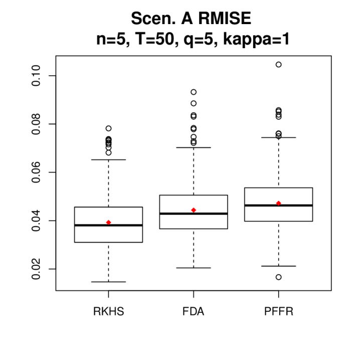
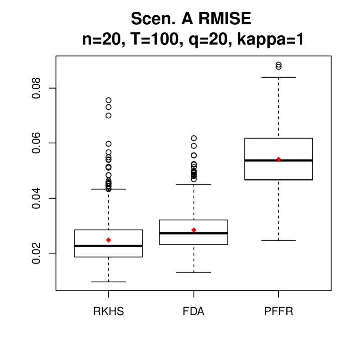
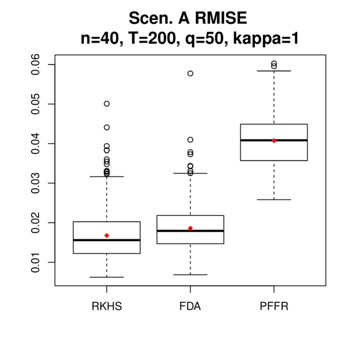
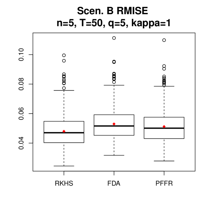
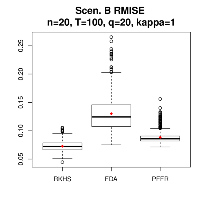
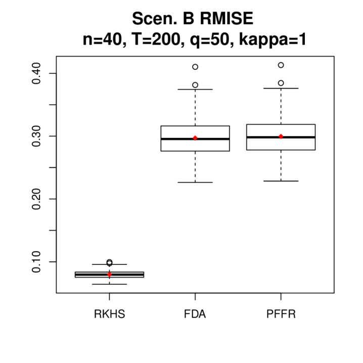
Figure 2: Boxplots of RMISE of RKHS, FDA and PFFR across 500 experiments under function-on-function regression with $\kappa=1$. Red points denote the average RMISE.

5.3 Functional regression with mixed predictors

In this subsection, we set $p=3$ and compare the performance of RKHS with PFFR, as FDA cannot handle mixed predictors. For RKHS, we use the standard 5-fold CV to select the tuning parameter $(\lambda_{1},\lambda_{2},\lambda_{3})$ from the range $10^{(-4:1:0)}\times 10^{(-4:1:0)}\times 10^{(-1:1:3)}$ for Scenario A and from the range $10^{(-17:1:-13)}\times 10^{(-17:1:-13)}\times 10^{(-1:1:3)}$ for Scenario B. PFFR uses REML to automatically select the roughness penalty and we set $N_{b}=20$ for PFFR as before.

Numerical results: Table 2 reports the average nRMISE (nRMISE_avg) across 500 experiments for RKHS and PFFR under all simulation settings. Table 2 further reports R_avg, the percentage improvement of RKHS over PFFR, and R_w, the percentage of experiments (among 500 experiments) where RKHS returns lower RMISE. We further give the boxplot of RMISE in Figure 3 under $\kappa=1$. The boxplots of RMISE under $\kappa=0.5,2$ can be found in Section G. The result is consistent with the one for function-on-function regression, where RKHS delivers the best performance across almost all simulation settings with notable improvement.

	Scenario A: $n=5,T=50,q=5$				Scenario B: $n=5,T=50,q=5$
$\kappa$	RKHS	PFFR	Ravg(%)	Rw (%)	RKHS	PFFR	Ravg(%)	Rw (%)
$0.5$	17.16	20.14	17.35	77	14.81	15.99	8.02	70
$1$	9.43	10.89	15.53	76	7.42	7.97	7.46	75
$2$	5.03	5.60	11.35	74	3.72	3.99	7.29	75
	Scenario A: $n=20,T=100,q=20$				Scenario B: $n=20,T=100,q=20$
$\kappa$	RKHS	PFFR	Ravg(%)	Rw (%)	RKHS	PFFR	Ravg(%)	Rw (%)
$0.5$	11.25	21.95	95.11	100	23.95	25.74	7.48	63
$1$	5.95	11.25	89.31	100	11.83	14.44	22.03	90
$2$	3.38	5.94	75.77	100	5.92	7.85	32.47	99
	Scenario A: $n=40,T=200,q=50$				Scenario B: $n=40,T=200,q=50$
$\kappa$	RKHS	PFFR	Ravg(%)	Rw (%)	RKHS	PFFR	Ravg(%)	Rw (%)
$0.5$	8.50	15.76	85.46	99	27.52	77.13	180.22	100
$1$	4.36	8.02	84.03	100	14.23	76.19	435.38	100
$2$	2.33	4.16	78.36	100	8.20	75.99	827.09	100

Table 2: Numerical performance of RKHS and PFFR under functional regression with mixed predictors. The reported nRMISE_avg is multiplied by 100 in scale. R_avg reflects the percent improvement of RKHS over PFFR and R_w reflects the percentage of experiments in which RKHS achieves the lower RMISE.

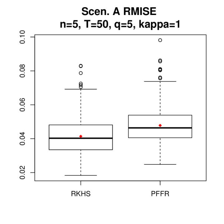
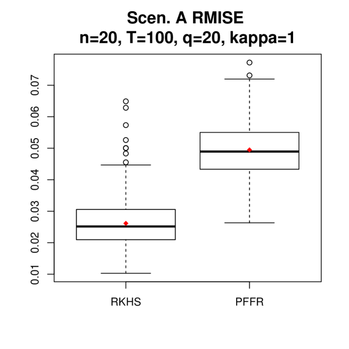
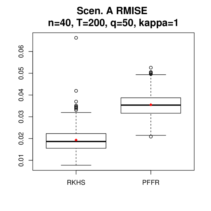
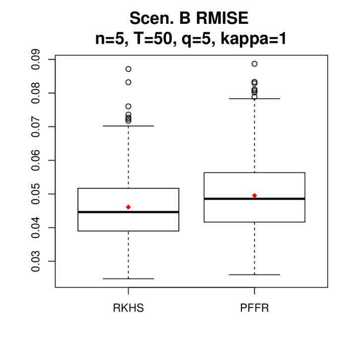
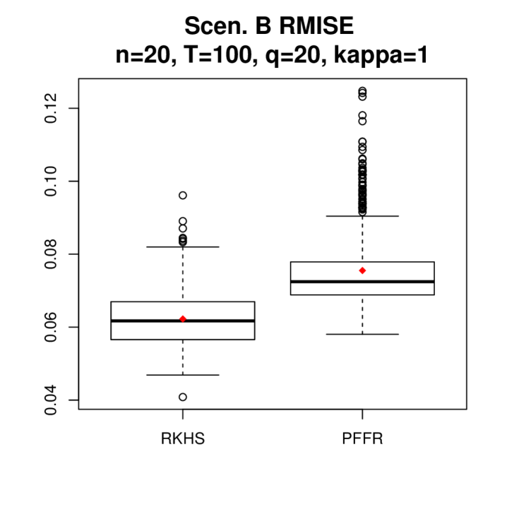
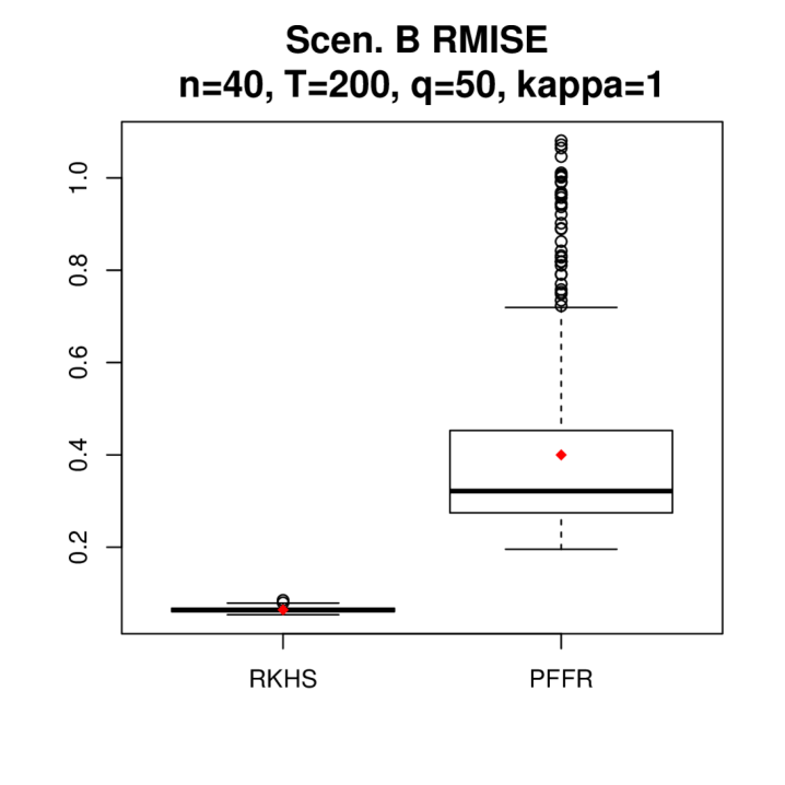
Figure 3: Boxplots of RMISE of RKHS and PFFR across 500 experiments under functional regression with mixed predictors with $\kappa=1$. Red points denote the average RMISE.

In the following, we further examine the performance of RKHS for high-dimensional scalar predictors. Specifically, keep the simulation setting identical as above, we increase the number of scalar predictors to $p=10,50,100,200$. As a reminder, the sparsity of $\beta^{*}=(\beta_{1}^{*},\beta_{2}^{*},\ldots,\beta_{p}^{*})$ is 1 as only $\beta_{1}^{*}$ is a non-zero function. In other words, the additionally introduced scalar predictors $(Z_{t2},Z_{t3},\ldots,Z_{tp})$ are purely noise. Thus, compared to the case of $p=3$, the performance of RKHS and PFFR are expected to worsen with an increasing dimension $p.$ However, thanks to the group Lasso-type penalty, which induces sparsity of the estimated coefficient functions $\widehat{\beta}$, we expect the excess risk of RKHS to grow at the rate of $O\big{(}\log(p)\big{)}$, as suggested in Theorem 2.

To conserve space, we present the result under the simulation setting with $(n,T,q)=(20,100,20)$ and $\kappa=1.$ Results under other settings are similar and thus omitted. Due to the lack of sparsity penalty, PFFR may not be suitable for the setting of high-dimensional predictors. For comparison, we only implement PFFR for $p=10$. Figure 4 (A) and (B) give the boxplot of RMISE for RKHS and PFFR across 500 experiments. As expected, the RMISE of RKHS increases as the dimension $p$ increases though at a rate slower than $p$. Indeed, RKHS at $p=200$ still gives better performance than PFFR at $p=10$. Figure 4 (C) gives the plot between average MISE across 500 experiments and $\log(p)$, where the relationship is seen to be roughly linear. This confirms that the excess risk of RKHS increases in the order of $O\big{(}\log(p)\big{)}$ as suggested in Theorem 2.

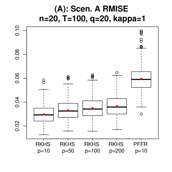
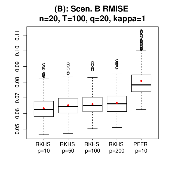
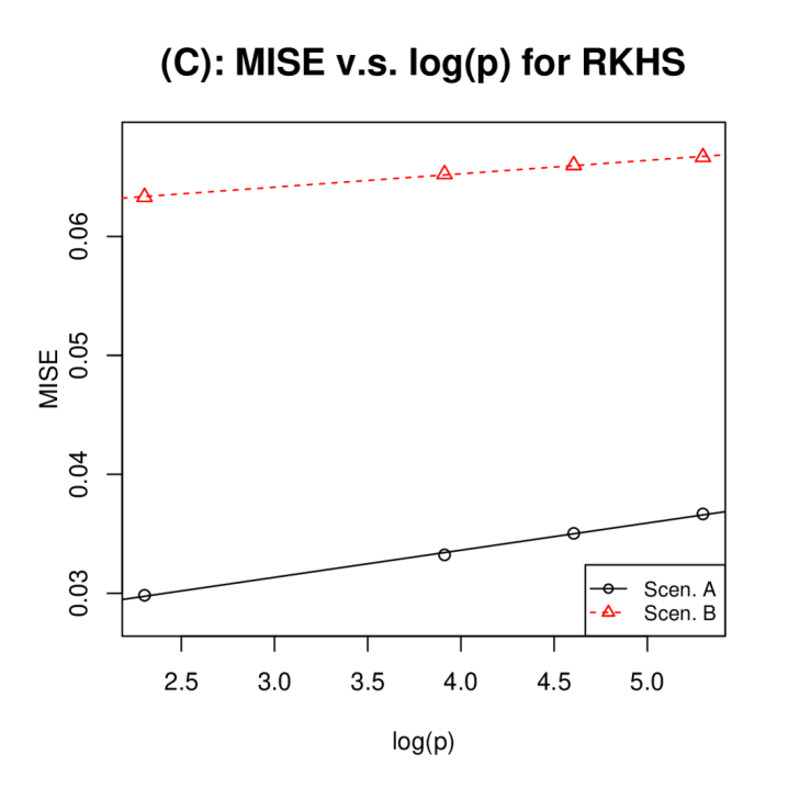
Figure 4: Boxplots of RMISE of RKHS and PFFR across 500 experiments under functional regression with mixed predictors with $\kappa=1$ for $p=10,50,100,200$. Red points denote the average RMISE. For plot (C), MISE = RMISE² and the two lines are fitted via OLS.

5.4 Real data applications

In this section, we conduct real data analysis to further demonstrate the promising utility of the proposed RKHS-based functional regression in the context of crowdfunding. In recent years, crowdfunding has become a flexible and cost-effective financing channel for start-ups and entrepreneurs, which helps expedite product development and diffusion of innovations.

We consider a novel dataset collected from one of the largest crowdfunding websites, kickstarter.com, which provides an online platform for creators, e.g. start-ups, to launch fundraising campaigns for developing a new product such as electronic devices and card games. The fundraising campaign takes place on a webpage set up by the creators, where information of the new product is provided, and typically has a 30-day duration with a goal amount $G$ preset by the creators. Over the course of the 30 days, backers can pledge funds to the campaign, resulting in a functional curve of pledged funds $\{P(r),r\in[0,30]\}$. At time $r$, the webpage displays real-time $P(r)$ along with other information of the campaign, such as its number of creators $Z_{1}$, number of product updates $Z_{2}$ and number of product FAQs $Z_{3}$.

A fundraising campaign succeeds if $P(30)\geq G$. Importantly, only creators of successful campaigns can be awarded the final raised funds $P(30)$ and the platform kickstarter.com charges a service fee ($5\%\times P(30)$) of successful campaigns. Thus, for both the platform and the creators, an accurate prediction of the future curve $\{P(r),r\in(s,30]\}$ at an early time $s$ is valuable, as it not only reveals whether the campaign will succeed but more importantly suggests timing along $(s,30]$ for potential intervention by the creators and the platform to boost the fundraising campaign and achieve greater revenue.

The dataset consists of $T=454$ campaigns launched between Dec-01-2019 and Dec-31-2019. For each campaign $t=1,\ldots,T$, we observe its normalized curve $N_{t}(r)=P_{t}(r)/G_{t}$ at 60 evenly spaced time points over its 30-day duration and denote it as $\{N_{t}(r_{i})\}_{i=1}^{60}$. See Figure 1 for normalized curves of six representative campaigns. At a time $s\in(0,30)$, to predict $\{N_{t}(r),r\in(s,30]\}$ for campaign $t$, we employ functional regression, where we treat $\{N_{t}(r_{i}),r_{i}\in(s,30]\}$ as the functional response $Y_{t}$, use $\{N_{t}(r_{i}),r_{i}\in[0,s]\}$ as the functional covariate $X_{t}$ and $(Z_{1},Z_{2},Z_{3})$ as the vector covariate. We compare the performances of RKHS, FDA and PFFR. Note that FDA only allows for one functional covariate, thus for RKHS and PFFR, we implement both the function-on-function regression and the functional regression with mixed predictors (denoted by RKHS${}_{\text{mixed}}$ and PFFR${}_{\text{mixed}}$). The implementation of each method is the same as that in Sections 5.2 and 5.3.

We vary the prediction time $s$ such that $s=7\text{th},8\text{th},\ldots,20\text{th}$ day of a campaign. Note that we stop at $s=20$ as prediction made in the late stage of a campaign is not as useful as early forecasts. To assess the out-of-sample performance of each method, we use a 2-fold CV, where we partition the 454 campaigns into two equal-sized sets and use one set to train the functional regression and the other to test the prediction performance, and then switch the role of the two sets. For each campaign $t$ in the test set, given its prediction $\{\widehat{N}_{t}(r),r\in(s,30]\}$ generated at time $s$, we calculate its RMSE and MAE with respect to the true value $\{N_{t}(r_{i}),r_{i}\in(s,30]\}$, where

$$\text{RMSE}_{t,s}=\sqrt{\frac{1}{\#\{r_{i}\in(s,30]\}}\sum_{r_{i}\in(s,30]}(\widehat{N}_{t}(r_{i})-N_{t}(r_{i}))^{2}}$$

and

$$\text{MAE}_{t,s}=\frac{1}{\#\{r_{i}\in(s,30]\}}\sum_{r_{i}\in(s,30]}\left|\widehat{N}_{t}(r_{i})-N_{t}(r_{i})\right|.$$

Figure 5 visualizes RMSE${}_{s}=T^{-1}\sum_{t=1}^{T}\text{RMSE}_{t,s}$ and MAE${}_{s}=T^{-1}\sum_{t=1}^{T}\text{MAE}_{t,s}$ achieved by different functional regression methods across $s\in\{7,8,\ldots,20\}.$ In general, the two RKHS-based estimators consistently achieve the best prediction accuracy. As expected, the performance of all methods improve with $s$ approaching 20. Interestingly, the functional regression with mixed predictors does not seem to improve the prediction performance, which is especially evident for PFFR. Thanks to the group Lasso-type penalty, RKHS can perform variable selection on the vector covariate. Indeed, among the 28 (2 folds $\times$ 14 days) estimated functional regression models based on RKHS${}_{\text{mixed}}$, 19 models select no vector covariate and thus reduce to the function-on-function regression, suggesting the potential irrelevance of the vector covariate. We further provide a robustness check of the above analysis in Section H, where we repeat the 2-fold CV procedure 100 times for RKHS, FDA and PFFR. It is seen that RKHS consistently provides the best performance, confirming the robustness of our findings. We refer to Section H for more details.

For more intuition, Figure 1 plots the normalized fundraising curves $\{N_{t}(r_{i})\}_{i=1}^{60}$ of six representative campaigns and further visualizes the functional predictions given by RKHS, FDA and PFFR at $s=14$th day. Note that FDA and RKHS provide more similar prediction while the prediction of PFFR seems to be more volatile. This is indeed consistent with the estimated bivariate coefficient functions visualized in Figure 6, where $\widehat{A}(r,s)$ of RKHS and FDA resembles each other while PFFR seems to suffer from under-smoothing.

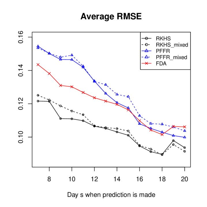
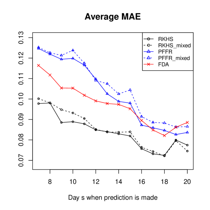
Figure 5: Average RMSE and MAE achieved by different functional regression methods.

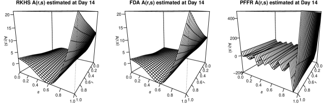
Figure 6: Estimated bivariate coefficient functions $\widehat{A}(r,s)$ by RKHS, FDA and PFFR at Day 14 ($(r,s)$ is rescaled to $[0,1]^{2}$).

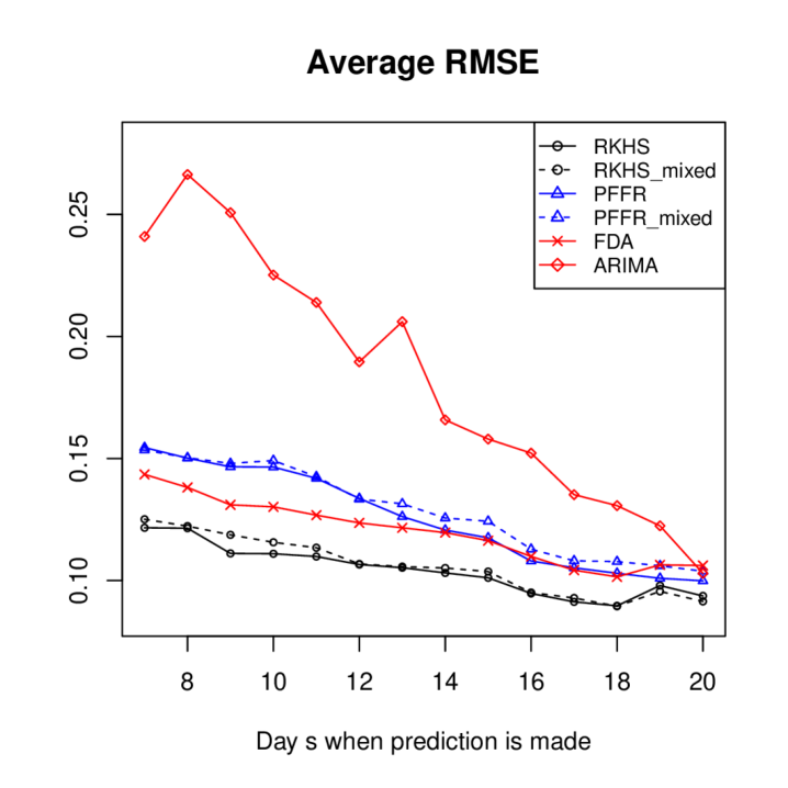
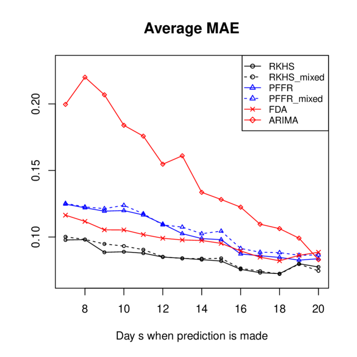
Figure 11: Average RMSE and MAE achieved by different functional regression methods. For campaign $t$ at prediction time $s$, ARIMA is trained on $\{N_{t}(r_{i}),r_{i}\in[0,s]\}$ for the prediction of $\{N_{t}(r_{i}),r_{i}\in(s,30]\}$. Note that ARIMA can be used as $\{N_{t}(r_{i})\}_{i=1}^{60}$ can be seen as an evenly spaced univariate time series.

Figure 11 in Section G further gives the prediction performance of the classical time series model ARIMA, which is significantly worse than the predictions given by RKHS, FDA and PFFR, suggesting the advantage of functional regression for handling the current application.

6 Conclusion

In this paper, we study a functional linear regression model with functional responses and accommodating both functional and high-dimensional vector covariates. We provide a minimax lower bound on its excess risk. To match the lower bound, we propose an RKHS-based penalized least squares estimator, which is based on a generalization of the representer lemma and achieves the optimal upper bound on the excess risk. Our framework allows for partially observed functional variables and provides finite sample probability bounds. Furthermore, the result unveils an interesting phase transition between a high-dimensional parametric rate and a nonparametric rate in terms of the excess risk. A novel iterative coordinate descent based algorithm is proposed to efficiently solve the penalized least squares problem. Simulation studies and real data applications are further conducted, where the proposed estimator is seen to provide favorable performance compared to existing methods in the literature.

Throughout the paper, we assume knowledge of the kernel functions $\mathbb{K}$ and $\mathbb{K}_{\beta}$. In practice, it would be ideal if one would be able to learn the kernel functions from data. However, to our best knowledge, assuming knowing the true kernel functions is adopted in all RKHS-based functional data analysis literature. Learning kernels is beyond the scope of our paper and we would like to pursue this direction in the future research. We would also like to point out that our estimator $(\widehat{A},\widehat{\beta})$ is a constrained estimator, with the constraints related with the true kernels. A mis-specification might lead to an over/under penalization, which will affect the final prediction error rate.

Finally, we briefly discuss important distinctions between non-parametric regression and functional regression for interested readers. To make the comparison easier, we consider a simpler setting: the scalar response functional linear regression and the classical non-parametric regression.

In non-parametric regression, we have

$$y_{i}=f(x_{i})+\epsilon_{i},$$

where $\{x_{i}\}_{i=1}^{n}$ are assumed to be random or fixed grid points in $[0,1]$. In scalar response functional linear regression with fully observed functional data, we have

$$y_{i}=\int X_{i}(s)\beta(s)\,\mathrm{d}s+\epsilon_{i},$$ (23)

where $\{X_{i}\}_{i=1}^{n}$ are assumed to be i.i.d. stochastic processes in $\mathcal{L}^{2}$. Note that we can treat $X_{i}$ and $\beta$ as infinite-dimensional vectors w.r.t. some $\mathcal{L}^{2}$ basis system, thus model (23) can be rewritten as

$$y_{i}=\widetilde{X}_{i}^{\top}\widetilde{\beta}+\epsilon_{i},$$

where $\widetilde{X}_{i}\in\mathbb{R}^{\infty},\widetilde{\beta}\in\mathbb{R}^{\infty}$. Under the standard assumption that $\mathbb{E}(\|X_{i}\|_{\mathcal{L}^{2}}^{2})<\infty$, the eigenvalue sequence of the covariance matrix $\widetilde{\Sigma}_{X}=\mathbb{E}(\widetilde{X}_{i}\widetilde{X}_{i}^{\top})$ converges to $0$. As such, model (23) was described as a high-dimensional or infinitely-dimensional “ill-posed” linear regression model in Hall and Horowitz (2007), which is fundamentally different from the standard non-parametric regression.

Appendices

Section A provides more discussions on the connection between bivariate functions and compact linear operators, Assumptions 2 and 3. Section B collects proofs of results in Section 3. Section C contains a series of deviation bounds, which are interesting per se. Section D contains the proof of Proposition 3. Section E includes additional details on technical proofs. Section F collects additional details on optimization. Additional numerical details are exhibited in Appendices G, H, I, J, K and L.

A More discussions on bivariate functions, Assumptions 2 and 3

A.1 Bivariate functions and compact linear operators

Remark 4

Fro any compact linear operator $A_{2}:{\mathcal{H}(\mathbb{K})}\to{\mathcal{H}(\mathbb{K})}$ denote

$$A_{2}[f,g]=\langle A_{2}[g],f\rangle_{\mathcal{H}(\mathbb{K})},\quad f,g\in{\mathcal{H}(\mathbb{K})}.$$

Note that $A_{2}[f,g]$ is well defined for any $f,g\in{\mathcal{H}(\mathbb{K})}$ due to the compactness of $A_{2}$. Define $a_{ij}=A_{2}[\psi_{i},\psi_{j}]=\langle A_{2}[\psi_{j}],\psi_{i}\rangle_{\mathcal{H}(\mathbb{K})}$, $i,j\in\mathbb{N}_{*}$. We thus have for any $f,g\in{\mathcal{H}(\mathbb{K})}$, it holds that

$$A_{2}[f,g] =\langle A_{2}[g],f\rangle_{\mathcal{H}(\mathbb{K})}=\sum_{i=1}^{\infty}\langle f,\psi_{i}\rangle_{{\mathcal{H}(\mathbb{K})}}\langle A_{2}[g],\psi_{i}\rangle_{{\mathcal{H}(\mathbb{K})}}$$

$$=\sum_{i=1}^{\infty}\langle f,\psi_{i}\rangle_{{\mathcal{H}(\mathbb{K})}}\Bigg{\langle}A_{2}\left[\sum_{j=1}^{\infty}\langle g,\psi_{j}\rangle_{{\mathcal{H}(\mathbb{K})}}\psi_{j}\right],\psi_{i}\Bigg{\rangle}_{{\mathcal{H}(\mathbb{K})}}$$

$$=\sum_{i,j=1}^{\infty}\langle f,\psi_{i}\rangle_{{\mathcal{H}(\mathbb{K})}}\langle g,\psi_{j}\rangle_{{\mathcal{H}(\mathbb{K})}}\langle A_{2}[\psi_{j}],\psi_{i}\rangle_{\mathcal{H}(\mathbb{K})}=\sum_{i,j=1}^{\infty}a_{ij}\langle f,\psi_{i}\rangle_{{\mathcal{H}(\mathbb{K})}}\langle g,\psi_{j}\rangle_{{\mathcal{H}(\mathbb{K})}},$$

where the fourth identity follows from the compactness of $A_{2}.$ This justifies Equation 2.

A.2 2(d)

In 2(d), we assume that

$$\mathbb{E}(\langle X_{1},f\rangle_{\mathcal{L}^{2}}Z^{\top}_{1}v)\leq\frac{3}{4}\sqrt{\mathbb{E}\{\langle X_{1},f\rangle_{\mathcal{L}^{2}}^{2}\}(v^{\top}\Sigma_{Z}v)},$$

i.e. the functional and vector covariates are allowed to be correlated up to $O(1)$. In this subsection, we emphasize that the correlation cannot be equal to one. We first note that

$$\mathbb{E}(\langle X_{1},f\rangle_{\mathcal{L}^{2}}Z^{\top}_{1}v)\leq\sqrt{\mathbb{E}\{\langle X_{1},f\rangle_{\mathcal{L}^{2}}^{2}\}(v^{\top}\Sigma_{Z}v)}.$$ (24)

For model identification, we require the inequality in (24) to be strict. To see this, we suppose that there exist $g\in{\mathcal{H}(\mathbb{K})}$ and $u\in\mathbb{R}^{p}$ such that

$$\mathbb{E}(\langle X_{1},g\rangle_{\mathcal{L}^{2}}Z^{\top}_{1}u)=\sqrt{\mathbb{E}\{\langle X_{1},g\rangle_{\mathcal{L}^{2}}^{2}\}(u^{\top}\Sigma_{Z}u)}.$$

Since $\langle X_{1},g\rangle_{\mathcal{L}^{2}}$ and $Z^{\top}_{1}u$ are both normal random variables, the above equality implies that the correlation between $\langle X_{1},g\rangle_{\mathcal{L}^{2}}$ and $Z^{\top}_{1}u$ is 1 and thus $\langle X_{1},g\rangle_{\mathcal{L}^{2}}=aZ^{\top}_{1}u$ for some constant $a\in\mathbb{R}$. This means that the model defined in (1) is no longer identifiable, because the covariates are perfectly correlated. Even in finite-dimensional regression problems, if the covariates are perfectly correlated, the solution to the linear system is ill-defined.

A.3 3(b)

Recall that 3 is required for handling the case where the functional observations are on discrete sample points. 3(a) formalizes the sampling scheme and 3(b) requires that the second moment of the random variable $\|X\|_{{W^{\alpha,2}}}$ is finite.

In the following, via a concrete example, we show that the second moment assumption in (7) holds under mild conditions. Specifically in Example 1, we provide a simple sufficient condition on the eigen-decay of the covariance operator $\Sigma_{X}$, under which (7) holds for $W^{\alpha,2}$ with $\alpha>1/2$.

Example 1

Let $\alpha>1/2$ and suppose the Sobolev space ${W^{\alpha,2}}$ is generated by the kernel

$$\mathbb{K}_{\alpha}(r,s)=\sum_{k=1}^{\infty}\omega_{k}\psi_{k}^{\alpha}(r)\psi_{k}^{\alpha}(s),$$

where due to the property of the Sobolev space, we have $\omega_{k}\asymp k^{-2\alpha}$ and $\{\psi_{k}^{\alpha}\}_{k=1}^{\infty}$ can be taken as the Fourier basis such that $\|\psi_{k}^{\alpha}\|_{W^{\alpha,2}}^{2}\asymp k^{2\alpha}$. To better understand the second moment condition

$$\mathbb{E}(\|X_{1}\|_{W^{\alpha,2}}^{2})<\infty,$$

we proceed by following the same strategy as in Cai and Hall (2006) and Yuan and Cai (2010) and assume that $\mathbb{K}_{\alpha}$ and $\Sigma_{X}$ are perfectly aligned, i.e., they share the same set of eigen-functions.

Let $z_{k}=\langle X_{1},\psi_{k}^{\alpha}\rangle_{\mathcal{L}^{2}}$. We have that $\{z_{k}\}_{k=1}^{\infty}$ is a collection of independent Gaussian random variables such that $z_{k}\sim N(0,\sigma_{k}^{2})$, where $\{\sigma_{k}^{2}\}_{k=1}^{\infty}$ are the eigenvalues of $\Sigma_{X}$. Thus we have

$$\|X_{1}\|_{W^{\alpha,2}}^{2}=\sum_{k=1}^{\infty}z_{k}^{2}\|\psi_{k}^{\alpha}\|_{W^{\alpha,2}}^{2}\asymp\sum_{k=1}^{\infty}z_{k}^{2}k^{2\alpha},$$

and

$$\mathbb{E}(\|X_{1}\|_{W^{\alpha,2}}^{2})\asymp\sum_{k=1}^{\infty}\mathbb{E}(z_{k}^{2})k^{2\alpha}=\sum_{k=1}^{\infty}\sigma_{k}^{2}k^{2\alpha}.$$

To assure that $\mathbb{E}(\|X_{1}\|_{W^{\alpha,2}}^{2})<\infty$, it suffices to have that

$$\sigma_{k}^{2}\asymp k^{-2\alpha-1-\nu}$$

for any constant $\nu>0$. Note that when $\alpha$ is close to $1/2$, this means that the eigenvalues of $\Sigma_{X}$ decay at a polynomial rate slightly faster than 2.

B Proofs of the results in Section 3

B.1 Proof of Proposition 1

Proof  [Proof of Proposition 1]

For any linear subspaces $R,S\subset{\mathcal{H}(\mathbb{K})}$, let $\mathcal{P}_{R}$ and $\mathcal{P}_{S}$ be the projection mappings of the spaces $R$ and $S$, respectively with respect to $\|\cdot\|_{\mathcal{H}(\mathbb{K})}$. For any $f,g\in{\mathcal{H}(\mathbb{K})}$ and any compact linear operator $A:{\mathcal{H}(\mathbb{K})}\to{\mathcal{H}(\mathbb{K})}$, denote

$$A|_{R\times S}[f,g]=A[\mathcal{P}_{R}f,\mathcal{P}_{S}g].$$

Let $(\widehat{B},\widehat{\alpha})$ be any solution to (3.1). Let $Q=\text{span}\{\mathbb{K}_{\beta}(r_{j},\cdot)\}_{j=1}^{n}\subset{\mathcal{H}(\mathbb{K}_{\beta})}$, $R=\text{span}\{\mathbb{K}(r_{j},\cdot)\}_{j=1}^{n}\subset{\mathcal{H}(\mathbb{K})}$ and $S=\text{span}\{\mathbb{K}(s_{j},\cdot)\}_{j=1}^{n}\subset{\mathcal{H}(\mathbb{K})}$. Denote $\widehat{\beta}_{l}=\mathcal{P}_{Q}(\widehat{\alpha}_{l})$, $l\in\{1,\ldots,p\}$, and $\widehat{A}[\cdot,\cdot]=\widehat{B}|_{R\times S}[\cdot,\cdot]=\widehat{B}[\mathcal{P}_{R}\cdot,\mathcal{P}_{S}\cdot]$.

Let $S^{\perp}$ and $R^{\perp}$ be the orthogonal complements of $S$ and $R$ in $\mathcal{H}$, respectively. Then for any compact linear operator $A$, we have the decomposition

$$A=A|_{R\times S}+A|_{R\times S^{\perp}}+A|_{R^{\perp}\times S}+A|_{R^{\perp}\times S^{\perp}}.$$

Due to Lemma 5, there exist $\{a_{ij}\}_{i,j=1}^{n}\subset\mathbb{R}$ such that

$$A|_{R\times S}[f,g]=\sum_{i,j=1}^{n}a_{ij}\langle\mathbb{K}(r_{i},\cdot),f\rangle_{\mathcal{H}(\mathbb{K})}\langle\mathbb{K}(s_{j},\cdot),g\rangle_{\mathcal{H}(\mathbb{K})}.$$

Step 1. In this step, it is shown that for any compact linear operator $A$, its associated bivariate function $A(\cdot,\cdot)$ satisfies that $\{A(r_{i},s_{j})\}_{i,j=1}^{n}$ only depend on $A|_{R\times S}$. The details of the bivariate function is explained in Section A.1.  
Observe that

$$A|_{R\times S^{\perp}}(r_{i},s_{j})=A|_{R\times S^{\perp}}[\mathbb{K}(r_{i},\cdot),\mathbb{K}(s_{j},\cdot)]=A[\mathcal{P}_{R}\mathbb{K}(r_{i},\cdot),\mathcal{P}_{S^{\perp}}\mathbb{K}(s_{j},\cdot)]=0.$$

Similar arguments also lead to that $A|_{R^{\perp}\times S}[\mathbb{K}(r_{i},\cdot),\mathbb{K}(s_{j},\cdot)]=0$ and $A|_{R^{\perp}\times S^{\perp}}[\mathbb{K}(r_{i},\cdot),\mathbb{K}(s_{j},\cdot)]=0$, $i,j=1,\ldots,n$.

Step 2. By Step 1, it holds that $\widehat{A}(r_{i},s_{j})=\widehat{B}(r_{i},s_{j})$, $i,j=1,\ldots,n$. By Lemma 5, we have that there exist $\{\widehat{a}_{ij}\}_{i,j=1}^{n}\subset\mathbb{R}$ such that for any $f,g\in{\mathcal{H}(\mathbb{K})}$,

$$\widehat{A}[f,g]=\sum_{i,j=1}^{n}\widehat{a}_{ij}\langle\mathbb{K}(r_{i},\cdot),f\rangle_{\mathcal{H}(\mathbb{K})}\langle\mathbb{K}(s_{j},\cdot),g\rangle_{\mathcal{H}(\mathbb{K})}.$$

Therefore the associated bivariate function satisfies that, for all $r,s\in[0,1]$,

$$\widehat{A}(r,s) =\sum_{i,j=1}^{\infty}\widehat{A}[\psi_{i},\psi_{j}]\psi_{i}(r)\psi_{j}(s)=\sum_{i,j=1}^{\infty}\sum_{k,l=1}^{n}\widehat{a}_{kl}\psi_{i}(r_{k})\psi_{j}(s_{l})\psi_{i}(r)\psi_{j}(s)$$

$$=\sum_{k,l=1}^{n}\widehat{a}_{kl}\left\{\sum_{i=1}^{\infty}\psi_{i}(r)\psi_{i}(r_{k})\right\}\left\{\sum_{i=1}^{\infty}\psi_{i}(s)\psi_{i}(s_{l})\right\}=\sum_{k,l=1}^{n}\widehat{a}_{kl}\mathbb{K}(r,r_{k})\mathbb{K}(s,s_{l}),$$

where $K(r,s)=\sum_{i=1}^{\infty}\psi(s)\psi(r)$ is used in the last inequality.

Step 3. For any $j\in\{1,\ldots,n\}$ and $l\in\{1,\ldots,p\}$, by the definition of $\widehat{\beta}_{l}$, we have that

$$\widehat{\alpha}_{l}(r_{j})=\langle\widehat{\alpha}_{l},\mathbb{K}_{\beta}(r_{j},\cdot)\rangle_{\mathcal{H}}=\langle\widehat{\beta}_{l},\mathbb{K}_{\beta}(r_{j},\cdot)\rangle_{\mathcal{H}}=\widehat{\beta}_{l}(r_{j}).$$

Therefore

$$\frac{1}{Tn}\sum_{t=1}^{T}\sum_{i=1}^{n}{w_{r}(i)}\left\{Y_{t}(r_{i})-\frac{1}{n}\sum_{j=1}^{n}{w_{s}(j)}\widehat{A}(r_{i},s_{j})X_{t}(s_{j})-\langle\widehat{\beta}(r_{i}),Z_{t}\rangle_{p}\right\}^{2}+\lambda\sum_{l=1}^{p}\|\widehat{\beta}_{l}\|_{n}$$

$$= \frac{1}{Tn}\sum_{t=1}^{T}\sum_{i=1}^{n}{w_{r}(i)}\left\{Y_{t}(r_{i})-\frac{1}{n}\sum_{j=1}^{n}{w_{s}(j)}\widehat{B}(r_{i},s_{j})X_{t}(s_{j})-\langle\widehat{\alpha}(r_{i}),Z_{t}\rangle_{p}\right\}^{2}+\lambda\sum_{l=1}^{p}\|\widehat{\alpha}_{l}\|_{n}.$$

In addition, by Lemma 5 we have that

$$\|\widehat{A}\|_{\mathrm{F}(\mathbb{K})}\leq\|\widehat{B}\|_{\mathrm{F}(\mathbb{K})}\quad\mbox{and}\quad\|\widehat{\beta}_{l}\|_{{\mathcal{H}(\mathbb{K}_{\beta})}}\leq\|\widehat{\alpha}_{l}\|_{{\mathcal{H}(\mathbb{K}_{\beta})}}\quad\text{ for all }l\in\{1,\ldots,p\},$$

which completes the proof.  

Lemma 5

Let $A:{\mathcal{H}(\mathbb{K})}\to{\mathcal{H}(\mathbb{K})}$ be any Hilbert–Schmidt operator. Let $\{v_{i},v^{\prime}_{i}\}_{i=1}^{m}\subset{\mathcal{H}(\mathbb{K})}$ be a collection of functions in ${\mathcal{H}(\mathbb{K})}$. Let $R$ and $S$ be the subspaces of ${\mathcal{H}(\mathbb{K})}$ spanned by $\{v_{i}\}_{i=1}^{m}$ and $\{v^{\prime}_{i}\}_{i=1}^{m}$, respectively. Let $\mathcal{P}_{R}$ and $\mathcal{P}_{S}$ be the projection mappings of the spaces $R$ and $S$, respectively. Then there exist $\{a_{ij}\}_{i,j=1}^{m}\subset\mathbb{R}$, which are not necessarily unique, such that for any $f,g\in{\mathcal{H}(\mathbb{K})}$,

$$A|_{R\times S}[f,g]=A[\mathcal{P}_{R}f,\mathcal{P}_{S}g]=\sum_{i,j=1}^{m}a_{ij}\langle f,v_{i}\rangle_{{\mathcal{H}(\mathbb{K})}}\langle g,v_{i}\rangle_{{\mathcal{H}(\mathbb{K})}},$$

and that $\|A|_{R\times S}[f,g]\|_{{\mathrm{F}(\mathbb{K})}}\leq\|A\|_{{\mathrm{F}(\mathbb{K})}}$.

Proof  Let $\{u_{k}\}_{k=1}^{K}$ and $\{u^{\prime}_{l}\}_{l=1}^{L}$ be orthogonal basis of subspaces $R$ and $S$ of $\mathcal{L}^{2}$, respectively, with $K,L\leq m$. Since each $u_{i}$($u^{\prime}_{i}$) can be written as a linear combination of $\{v_{k}\}_{k=1}^{m}$($\{v^{\prime}_{k}\}_{k=1}^{m}$), it suffices to show that there exist $\{b_{ij}\}_{i=1,j=1}^{K,L}\subset\mathbb{R}$, such that for any $f,g\in{\mathcal{H}(\mathbb{K})}$,

$$A|_{R\times S}[f,g]=\sum_{k=1}^{K}\sum_{l=1}^{L}b_{ij}\langle u_{i},f\rangle_{{\mathcal{H}(\mathbb{K})}}\langle u_{j}^{\prime},g\rangle_{{\mathcal{H}(\mathbb{K})}}.$$

Since $R$ and $S$ are linear subspaces of ${\mathcal{H}(\mathbb{K})}$, there exist $\{u_{k}\}_{k=K+1}^{\infty},\{u^{\prime}_{l}\}_{l=L+1}^{\infty}\subset{\mathcal{H}(\mathbb{K})}$, such that $\{u_{k}\}_{k=1}^{\infty}$ and $\{u_{l}^{\prime}\}_{l=1}^{\infty}$ are two orthogonal basis of ${\mathcal{H}(\mathbb{K})}$, and that

$$A[f,g]=\sum_{i,j=1}^{\infty}b_{ij}\langle u_{i},f\rangle_{{\mathcal{H}(\mathbb{K})}}\langle u_{j}^{\prime},g\rangle_{{\mathcal{H}(\mathbb{K})}},$$

where $b_{ij}=A[u_{i},u_{j}^{\prime}]=\langle A[u_{j}^{\prime}],u_{i}\rangle_{\mathcal{H}(\mathbb{K})}$. Therefore

$$A|_{R\times S}[f,g]= \sum_{i,j=1}^{\infty}b_{ij}\langle u_{i},\mathcal{P}_{R}f\rangle_{{\mathcal{H}(\mathbb{K})}}\langle u_{j}^{\prime},\mathcal{P}_{S}g\rangle_{{\mathcal{H}(\mathbb{K})}}=\sum_{i,j=1}^{\infty}b_{ij}\langle\mathcal{P}_{R}u_{i},f\rangle_{{\mathcal{H}(\mathbb{K})}}\langle\mathcal{P}_{S}u_{j}^{\prime},g\rangle_{{\mathcal{H}(\mathbb{K})}}$$

$$= \sum_{k=1}^{K}\sum_{l=1}^{L}b_{kl}\langle u_{k},f\rangle_{{\mathcal{H}(\mathbb{K})}}\langle u_{l}^{\prime},g\rangle_{{\mathcal{H}(\mathbb{K})}}.$$

Moreover, we have that

$$\|A\|_{\mathrm{F}(\mathbb{K})}^{2}=\sum_{k,l=1}^{\infty}b_{kl}^{2}\geq\sum_{k=1}^{K}\sum_{l=1}^{L}b_{kl}^{2}=\|A|_{R\times S}\|_{\mathrm{F}(\mathbb{K})}^{2},$$

which concludes the proof.  

B.2 Proof of Theorem 2

Proof [Proof of Theorem 2]

First note that $0<\delta_{T},\zeta_{n}<1$, then $\delta_{T}^{2}\leq\delta_{T}$ and $\zeta_{n}^{2}\leq\zeta_{n}$. These inequalities will be used repeatedly in the rest of this proof. Recall the notation that $\Delta_{\beta}(r)=\widehat{\beta}(r)-\beta^{*}(r)$ and $\Delta_{A}(r,s)=\widehat{A}(r,s)-A^{*}(r,s)$, $r,s\in[0,1]$. Note that for any $g\in{\mathcal{L}^{2}}$, it holds that

$$\mathbb{E}(\langle g,X^{*}\rangle_{\mathcal{L}^{2}}^{2})=\iint_{[0,1]^{2}}g(r)\Sigma_{X}(r,s)g(s)\,\mathrm{d}r\,\mathrm{d}s.$$

The above expression will also be used repeatedly in the rest of the proof. Observe that for any $r\in[0,1]$, it holds that

$$\|\Delta_{A}(r,\cdot)\|_{W^{\alpha,2}}\leq\|\Delta(r,\cdot)\|_{{\mathcal{H}(\mathbb{K})}}\leq C_{\mathbb{K}}\|\Delta\|_{{\mathrm{F}(\mathbb{K})}}\leq C_{\mathbb{K}}C_{A},$$

where the first inequality follows from 3 b, which assumes that ${\mathcal{H}(\mathbb{K})}\subset W^{\alpha,2}$, the second inequality follows from Lemma 30 and the last inequality follows from the assumption that $A^{*},\widehat{A}\in\mathcal{C}_{A}$. Throughout the proof, we assume without loss of generality that $C_{\mathbb{K}}=1.$ In addition, observe that by Lemma 27, it holds that

$$\mathbb{P}\big{(}\|X_{t}\|_{W^{\alpha,2}}\geq 4C_{X}\sqrt{\log(T)}\big{)}\leq T^{-6}.$$

By a union bound argument,

$$\mathbb{P}(\mathcal{D})=\mathbb{P}\big{(}\|X_{t}\|_{W^{\alpha,2}}\geq 4C_{X}\sqrt{\log(T)}\ \text{for all }1\leq t\leq T\big{)}\leq T^{-5}.$$

The rest of the proof is shown in the event of $\mathcal{D}$.

Let $\lambda=C_{\lambda}\sqrt{\frac{\log(p\vee T)}{T}}$ for sufficiently large constant $C_{\lambda}$. From the minimizer property, we have that

$$\frac{1}{Tn}\sum_{t=1}^{T}\sum_{i=1}^{n}{w_{r}(i)}\left\{Y_{t}(r_{i})-\frac{1}{n}\sum_{j=1}^{n}{w_{s}(j)}\widehat{A}(r_{i},s_{j})X_{t}(s_{j})-\langle Z_{t},\widehat{\beta}(r_{i})\rangle_{p}\right\}^{2}+\lambda\sum_{j=1}^{p}\|\widehat{\beta}_{j}\|_{n}$$

$$\leq \frac{1}{Tn}\sum_{t=1}^{T}\sum_{i=1}^{n}{w_{r}(i)}\left\{Y_{t}(r_{i})-\frac{1}{n}\sum_{j=1}^{n}{w_{s}(j)}A^{*}(r_{i},s_{j})X_{t}(s_{j})-\langle Z_{t},\beta^{*}(r_{i})\rangle_{p}\right\}^{2}+\lambda\sum_{j=1}^{p}\|\beta_{j}^{*}\|_{n},$$

which implies that

$$\frac{1}{Tn}\sum_{t=1}^{T}\sum_{i=1}^{n}{w_{r}(i)}\left\{\frac{1}{n}\sum_{j=1}^{n}{w_{s}(j)}\Delta_{A}(r_{i},s_{j})X_{t}(s_{j})\right\}^{2}$$ (25)

$$+ \frac{1}{Tn}\sum_{t=1}^{T}\sum_{i=1}^{n}{w_{r}(i)}\langle\Delta_{\beta}(r_{i}),Z_{t}\rangle^{2}_{p}$$ (26)

$$+ \frac{2}{Tn}\sum_{t=1}^{T}\sum_{i=1}^{n}{w_{r}(i)}\left\{\frac{1}{n}\sum_{j=1}^{n}{w_{s}(j)}\Delta_{A}(r_{i},s_{j})X_{t}(s_{j})\langle\Delta_{\beta}(r_{i}),Z_{t}\rangle_{p}\right\}$$ (27)

$$\leq \frac{2}{Tn}\sum_{t=1}^{T}\sum_{i=1}^{n}{w_{r}(i)}\left(\frac{1}{n}\sum_{j=1}^{n}{w_{s}(j)}\Delta_{A}(r_{i},s_{j})X_{t}(s_{j})+\langle\Delta_{\beta}(r_{i}),Z_{t}\rangle_{p}\right)\epsilon_{t}(r_{i})$$ (28)

$$+ \lambda\sum_{j=1}^{p}\|\beta_{j}^{*}\|_{n}-\lambda\sum_{j=1}^{p}\|\widehat{\beta}_{j}\|_{n}.$$ (29)

In the rest of the proof, for readability, we will assume that

$${w_{r}(i)}=1\text{ for all }1\leq i\leq n\quad\text{and}\quad{w_{s}(j)}=1\text{ for all }1\leq j\leq n.$$

This assumption is equivalent to the case that $\{r_{i}\}_{i=1}^{n}$ and $\{s_{j}\}_{j=1}^{n}$ are equally spaced grid. We note that in view of Lemma 33, the general case follows straightforwardly from the same argument and thus will be omitted for readability.

Step 1. Observe that

$$\eqref{eq:CAFR term 2}= \frac{2}{Tn}\sum_{t=1}^{T}\sum_{i=1}^{n}\left\{\frac{1}{n}\sum_{j=1}^{n}\Delta_{A}(r_{i},s_{j})X_{t}(s_{j})-\int_{[0,1]}\Delta_{A}(r_{i},s)X_{t}(s)\,\mathrm{d}s\right\}\langle\Delta_{\beta}(r_{i}),Z_{t}\rangle_{p}$$ (30)

$$\hskip 56.9055pt+\frac{2}{Tn}\sum_{t=1}^{T}\sum_{i=1}^{n}\left\{\int_{[0,1]}\Delta_{A}(r_{i},s)X_{t}(s)\,\mathrm{d}s\right\}\langle\Delta_{\beta}(r_{i}),Z_{t}\rangle_{p}.$$ (31)

As for the term (30), we have that for any $j\in\{1,\ldots,n\}$ and $t\in\{1,\ldots,T\}$,

$$\|\Delta_{A}(r_{j},\cdot)X_{t}(\cdot)\|_{{W^{\alpha,2}}}\leq\|\Delta_{A}(r_{j},\cdot)\|_{W^{\alpha,2}}\|X_{t}\|_{W^{\alpha,2}}\leq 8C_{A}C_{X}\sqrt{\log(T)},$$

where the first inequality follows from Lemma 34 and event $\mathcal{D}$. By Lemma 33, it holds that for all $1\leq i\leq n,1\leq t\leq T$,

$$\bigg{|}\frac{1}{n}\sum_{j=1}^{n}\Delta_{A}(r_{i},s_{j})X_{t}(s_{j})-\int_{[0,1]}\Delta_{A}(r_{i},s)X_{t}(s)\,\mathrm{d}s\bigg{|}\leq C_{1}\zeta_{n}\sqrt{\log(T)}$$

where $\zeta_{n}=n^{-\alpha+1/2}$ and $C_{1}$ depends on $C_{A}$ and $C_{X}$ only. So,

$$\eqref{eq:CAFR term 21}\geq -\frac{C_{1}}{Tn}\sum_{t=1}^{T}\sum_{i=1}^{n}\zeta_{n}\sqrt{\log(T)}\left|\langle\Delta_{\beta}(r_{i}),Z_{t}\rangle_{p}\right|$$

$$\geq -C_{1}\zeta_{n}\sqrt{\log(T)}\sqrt{\frac{1}{Tn}\sum_{t=1}^{T}\sum_{i=1}^{n}\langle\Delta_{\beta}(r_{i}),Z_{t}\rangle_{p}^{2}}$$

$$\geq -\frac{1}{640Tn}\sum_{t=1}^{T}\sum_{i=1}^{n}\langle\Delta_{\beta}(r_{i}),Z_{t}\rangle_{p}^{2}-640C_{1}^{2}\zeta_{n}^{2}\log(T)$$

$$= -\frac{1}{640Tn}\sum_{t=1}^{T}\sum_{i=1}^{n}\langle\Delta_{\beta}(r_{i}),Z_{t}\rangle_{p}^{2}-C_{1}^{\prime}\zeta_{n}^{2}\log(T),$$

for some absolute constant $C^{\prime}_{1}>0$.

In addition, for Equation 31, note that with probability at least $1-(p\vee T)^{-4}$,

$$\left\{\int_{[0,1]}\Delta_{A}(r_{i},s)\frac{1}{T}\sum_{t=1}^{T}X_{t}(s)Z_{t}^{\top}\Delta_{\beta}(r_{i})\,\mathrm{d}s\right\}-\left\{\int_{[0,1]}\Delta_{A}(r_{i},s)\mathbb{E}\{X_{t}(s)Z_{t}^{\top}\}\Delta_{\beta}(r_{i})\,\mathrm{d}s\right\}$$

$$= \int_{[0,1]}\Delta_{A}(r_{i},s)\bigg{(}\frac{1}{T}\sum_{t=1}^{T}X_{t}(s)Z_{t}^{\top}-\mathbb{E}\{X_{t}(s)Z_{t}^{\top}\}\bigg{)}\Delta_{\beta}(r_{i})\,\mathrm{d}s$$

$$\geq -\|\Delta_{A}(r_{i},\cdot)\|_{\mathcal{L}^{2}}\bigg{\|}\bigg{(}\frac{1}{T}\sum_{t=1}^{T}X_{t}(s)Z_{t}^{\top}-\mathbb{E}\{X_{t}(s)Z_{t}^{\top}\}\bigg{)}\Delta_{\beta}(r_{i})\bigg{\|}_{\mathcal{L}^{2}}$$

$$\geq -2C_{A}\sum_{1\leq j\leq p}\bigg{\|}\frac{1}{T}\sum_{t=1}^{T}X_{t}(s)Z_{t,j}^{\top}-\mathbb{E}\{X_{t}(s)Z_{t,j}^{\top}\}\bigg{\|}_{\mathcal{L}^{2}}|\Delta_{\beta_{j}}(r_{i})|$$

$$\geq -2C_{A}\sum_{1\leq j\leq p}|\Delta_{\beta_{j}}(r_{i})|\max_{1\leq j\leq p}\bigg{\|}\frac{1}{T}\sum_{t=1}^{T}X_{t}(s)Z_{t,j}^{\top}-\mathbb{E}\{X_{t}(s)Z_{t,j}^{\top}\}\bigg{\|}_{\mathcal{L}^{2}}$$

$$\geq -C_{1}^{\prime}\sum_{1\leq j\leq p}|\Delta_{\beta_{j}}(r_{i})|\sqrt{\frac{\log(p)}{T}}\geq-\frac{\lambda}{200}\sum_{1\leq j\leq p}|\Delta_{\beta_{j}}(r_{i})|,$$ (32)

where the second inequality holds because $\|\Delta_{A}(r_{i},\cdot)\|_{\mathcal{L}^{2}}\leq\|\Delta_{A}(r_{i},\cdot)\|_{\mathcal{H}(\mathbb{K})}\leq 2C_{A}$, the fourth inequality follows from Lemma 28, and the last inequality follows from the assumption that $\lambda=C_{\lambda}\sqrt{\frac{\log(p\vee T)}{T}}$ with sufficiently large $C_{\lambda}$. In addition, by 2(c),

$$\int_{[0,1]}-\Delta_{A}(r_{i},s)\mathbb{E}\{X_{t}(s)Z_{t}^{\top}\}\Delta_{\beta}(r_{i})\,\mathrm{d}s$$

$$\leq \frac{3}{4}\sqrt{\Sigma_{X}[\Delta_{A}(r_{i},\cdot),\Delta_{A}(r_{i},\cdot)]}\sqrt{\Delta_{\beta}(r_{i})^{\top}\Sigma_{Z}\Delta_{\beta}(r_{i})}$$

$$\leq \frac{3}{8}\bigg{(}\frac{6}{5}\Sigma_{X}[\Delta_{A}(r_{i},\cdot),\Delta_{A}(r_{i},\cdot)]+\frac{5}{6}\Delta_{\beta}(r_{i})^{\top}\Sigma_{Z}\Delta_{\beta}(r_{i})\bigg{)}$$

$$= \frac{9}{20}\Sigma_{X}[\Delta_{A}(r_{i},\cdot),\Delta_{A}(r_{i},\cdot)]+\frac{5}{16}\Delta_{\beta}(r_{i})^{\top}\Sigma_{Z}\Delta_{\beta}(r_{i})$$

$$= \frac{9}{20}\iint_{[0,1]^{2}}\Delta_{A}(r_{i},r)\Sigma_{X}(r,s)\Delta_{A}(r_{i},s)\,\mathrm{d}r\,\mathrm{d}s+\frac{5}{16}\Delta_{\beta}(r_{i})^{\top}\Sigma_{Z}\Delta_{\beta}(r_{i}).$$

So

$$\eqref{eq:CAFR term 22}$$

$$\geq -\frac{\lambda}{100}\frac{1}{n}\sum_{i=1}^{n}\sum_{j=1}^{p}|\Delta_{\beta_{j}}(r_{i})|-\frac{1}{n}\sum_{i=1}^{n}\frac{9}{10}\iint_{[0,1]^{2}}\Delta_{A}(r_{i},r)\Sigma_{X}(r,s)\Delta_{A}(r_{i},s)\,\mathrm{d}r\,\mathrm{d}s-\frac{1}{n}\sum_{i=1}^{n}\frac{5}{8}\Delta_{\beta}(r_{i})^{\top}\Sigma_{Z}\Delta_{\beta}(r_{i})$$

$$\geq -\frac{\lambda}{100}\sum_{j=1}^{p}\|\Delta_{\beta_{j}}\|_{n}-\frac{1}{n}\sum_{i=1}^{n}\frac{9}{10}\iint_{[0,1]^{2}}\Delta_{A}(r_{i},r)\Sigma_{X}(r,s)\Delta_{A}(r_{i},s)\,\mathrm{d}r\,\mathrm{d}s-\frac{1}{n}\sum_{i=1}^{n}\frac{5}{8}\Delta_{\beta}(r_{i})^{\top}\Sigma_{Z}\Delta_{\beta}(r_{i})$$

$$= -\frac{\lambda}{100}\big{(}\sum_{j\in S}\|\Delta_{\beta_{j}}\|_{n}+\sum_{j\in S^{c}}\|\widehat{\beta}_{j}\|_{n}\big{)}$$

$$- \frac{1}{n}\sum_{i=1}^{n}\frac{9}{10}\iint_{[0,1]^{2}}\Delta_{A}(r_{i},r)\Sigma_{X}(r,s)\Delta_{A}(r_{i},s)\,\mathrm{d}r\,\mathrm{d}s-\frac{1}{n}\sum_{i=1}^{n}\frac{5}{8}\Delta_{\beta}(r_{i})^{\top}\Sigma_{Z}\Delta_{\beta}(r_{i})$$

Putting calculations for Equation 30 and Equation 31 together, we have that

$$\eqref{eq:CAFR term 2}\geq -\frac{1}{640Tn}\sum_{t=1}^{T}\sum_{i=1}^{n}\langle\Delta_{\beta}(r_{i}),Z_{t}\rangle_{p}^{2}-C_{1}^{\prime}\zeta_{n}^{2}\log(T)-\frac{\lambda}{100}\big{(}\sum_{j\in S}\|\Delta_{\beta_{j}}\|_{n}+\sum_{j\in S^{c}}\|\widehat{\beta}_{j}\|_{n}\big{)}$$

$$- \frac{1}{n}\sum_{i=1}^{n}\frac{9}{10}\iint_{[0,1]^{2}}\Delta_{A}(r_{i},r)\Sigma_{X}(r,s)\Delta_{A}(r_{i},s)\,\mathrm{d}r\,\mathrm{d}s-\frac{1}{n}\sum_{i=1}^{n}\frac{5}{8}\Delta_{\beta}(r_{i})^{\top}\Sigma_{Z}\Delta_{\beta}(r_{i}).$$ (33)

Step 2. It follows from (43) that with probability at least $1-T^{-4}$, it holds that

$$\eqref{eq:CAFR term 0}\geq \frac{159}{160n}\sum_{i=1}^{n}\iint_{[0,1]^{2}}\Delta_{A}(r_{i},r)\Sigma(r,s)\Delta_{A}(r_{i},s)\,\mathrm{d}r\,\mathrm{d}s-C_{2}\left(\log(T)\zeta_{n}^{2}+\log(T)\delta_{T}\right),$$ (34)

where $C_{2}>0$ is an absolute constant.

It follows from (47) and (51), we have that with probability at least $1-2T^{-4}$, it holds that

$$\eqref{eq:CAFR term 4}\leq \frac{1}{320n}\sum_{i=1}^{n}\iint_{[0,1]^{2}}\Delta_{A}(r_{i},r)\Sigma_{X}(r,s)\Delta_{A}(r_{i},s)\,\mathrm{d}r\,\mathrm{d}s+C_{2}^{\prime}\Bigg{\{}\zeta_{n}+\log(T)\delta_{T}\Bigg{\}}$$

$$+ \frac{\lambda}{320}\sum_{j\in S}\|\Delta_{\beta_{j}}\|_{n}+\frac{\lambda}{320}\sum_{j\in S^{c}}\|\widehat{\beta}_{j}\|_{n}$$

where $C_{2}^{\prime}>0$ is an absolute constant.

Step 3. Note that for Equation 29,

$$\lambda\sum_{j=1}^{p}\|\beta_{j}^{*}\|_{n}-\sum_{j=1}^{p}\lambda\|\widehat{\beta}_{j}\|_{n}= \lambda\bigg{\{}\sum_{j\in S}\|\beta_{j}^{*}\|_{n}-\sum_{j\in S}\|\widehat{\beta}_{j}\|_{n}-\sum_{j\in S^{c}}\|\widehat{\beta}_{j}\|_{n}\bigg{\}}$$

$$\leq \lambda\sum_{j\in S}\|\Delta_{\beta_{j}}\|_{n}-\lambda\sum_{j\in S^{c}}\|\widehat{\beta}_{j}\|_{n}.$$

Step 4. Putting all previous calculations together leads to that

$$\frac{31}{320n}\sum_{i=1}^{n}\iint_{[0,1]^{2}}\Delta_{A}(r_{i},r)\Sigma_{X}(r,s)\Delta_{A}(r_{i},s)\,\mathrm{d}r\,\mathrm{d}s$$

$$+ \frac{639}{640Tn}\sum_{t=1}^{T}\sum_{i=1}^{n}\langle\Delta_{\beta}(r_{i}),Z_{t}\rangle_{p}^{2}-\frac{5}{8n}\sum_{i=1}^{n}\Delta_{\beta}(r_{i})^{\top}\Sigma_{Z}\Delta_{\beta}(r_{i})$$ (35)

$$\leq \big{(}1+\frac{1}{100}+\frac{1}{320}\big{)}\lambda\sum_{j\in S}\|\Delta_{\beta_{j}}\|_{n}-\lambda\big{(}1-\frac{1}{100}-\frac{1}{320}\big{)}\sum_{j\in S^{c}}\|\widehat{\beta}_{j}\|_{n}+C_{3}\big{\{}\log(T)\zeta_{n}+\log(T)\delta_{T}\big{\}},$$

$$\leq 2\lambda\sum_{j\in S}\|\Delta_{\beta_{j}}\|_{n}+C_{3}\big{\{}\log(T)\zeta_{n}+\log(T)\delta_{T}\big{\}}$$ (36)

where $C_{3}>0$ is some absolute constant.

For Equation 35, note that by constrain set $\mathcal{C}_{\beta}$, we have that

$$\sum_{1\leq j\leq p}\|\widehat{\beta}_{j}\|_{n}\leq\sum_{1\leq j\leq p}\|\widehat{\beta}_{j}\|_{\infty}\leq\sum_{1\leq j\leq p}\|\widehat{\beta}_{j}\|_{\mathcal{H}(\mathbb{K}_{\beta})}\leq C_{\beta}.$$

Therefore

$$\sum_{1\leq j\leq p}\|\Delta_{\beta_{j}}\|_{n}\leq\sum_{1\leq j\leq p}\|\widehat{\beta}_{j}\|_{n}+\sum_{1\leq j\leq p}\|\beta_{j}^{*}\|_{n}\leq 2C_{\beta}.$$

From Theorem 21, it holds that with probability at least $1-\exp(-cT)$,

$$\frac{639}{640T}\sum_{t=1}^{T}\langle\Delta_{\beta}(r_{i}),Z_{t}\rangle_{p}^{2}\geq \frac{639}{640}\cdot\frac{2}{3}\Delta_{\beta}(r_{i})^{\top}\Sigma_{Z}\Delta_{\beta}(r_{i})-C_{3}^{\prime}\frac{\log(p)}{T}\bigg{(}\sum_{1\leq j\leq p}\|\Delta_{\beta_{j}}\|_{n}\bigg{)}^{2}$$

$$\geq \frac{213}{320}\Delta_{\beta}(r_{i})^{\top}\Sigma_{Z}\Delta_{\beta}(r_{i})-4C_{3}^{\prime}C_{\beta}^{2}\frac{\log(p)}{T}.$$

Substitute the above inequality into Equation 35 gives

$$\frac{31}{320n}\sum_{i=1}^{n}\iint_{[0,1]^{2}}\Delta_{A}(r_{i},r)\Sigma_{X}(r,s)\Delta_{A}(r_{i},s)\,\mathrm{d}r\,\mathrm{d}s$$

$$+ \frac{13}{320n}\sum_{i=1}^{n}\Delta_{\beta}(r_{i})^{\top}\Sigma_{Z}\Delta_{\beta}(r_{i})$$

$$\leq 2\lambda\sum_{j\in S}\|\Delta_{\beta_{j}}\|_{n}$$ (37)

$$+ C_{3}^{\prime\prime}\big{\{}\log(T)\zeta_{n}+\log(T)\delta_{T}+\frac{\log(p)}{T}\big{\}}.$$

Step 5. Note that by 2c,

$$\left(\lambda\sum_{j\in S}\|\Delta_{\beta_{j}}\|_{n}\right)^{2}\leq\lambda^{2}\mathfrak{s}\sum_{j=1}^{p}\|\Delta_{\beta_{j}}\|_{n}^{2}=\lambda^{2}\mathfrak{s}\frac{1}{n}\sum_{i=1}^{n}\sum_{j=1}^{p}\{\Delta_{\beta_{j}}(r_{i})\}^{2}\leq\frac{\lambda^{2}\mathfrak{s}}{c_{z}}\frac{1}{n}\sum_{i=1}^{n}\Delta_{\beta}(r_{i})^{\top}\Sigma_{Z}\Delta_{\beta}(r_{i}),$$

where $\mathfrak{s}=|S|$, the cardinality of the support set $S$. This gives

$$\sum_{j\in S}\|\Delta_{\beta_{j}}\|_{n}\leq\sqrt{\frac{\mathfrak{s}}{c_{z}}\frac{1}{n}\sum_{i=1}^{n}\Delta_{\beta}(r_{i})^{\top}\Sigma_{Z}\Delta_{\beta}(r_{i})},$$ (38)

which implies that

$$\frac{1}{160}\lambda\sum_{j\in S}\|\Delta_{\beta_{j}}\|_{n}\leq \frac{1}{320n}\sum_{i=1}^{n}\Delta_{\beta}(r_{i})^{\top}\Sigma_{Z}\Delta_{\beta}(r_{i})+C_{4}\mathfrak{s}\lambda^{2}$$

$$\leq \frac{1}{320n}\sum_{i=1}^{n}\Delta_{\beta}(r_{i})^{\top}\Sigma_{Z}\Delta_{\beta}(r_{i})+C_{4}C_{\lambda}^{2}\frac{\mathfrak{s}\log(p\vee T)}{T}.$$

Substituting the above inequality into (37) gives

$$\frac{31}{320n}\sum_{i=1}^{n}\iint_{[0,1]^{2}}\Delta_{A}(r_{i},r)\Sigma_{X}(r,s)\Delta_{A}(r_{i},s)\,\mathrm{d}r\,\mathrm{d}s+\frac{12}{320n}\sum_{i=1}^{n}\Delta_{\beta}(r_{i})^{\top}\Sigma_{Z}\Delta_{\beta}(r_{i})$$

$$\leq C_{4}^{\prime}\big{\{}\log(T)\zeta_{n}+\log(T)\delta_{T}+\frac{\log(p)}{T}+\frac{\mathfrak{s}\log(p\vee T)}{T}\big{\}}$$ (39)

Step 6. Note that by definition, $\mathcal{E}^{*}(\widehat{A},\widehat{\beta})\geq 0$ for any estimators $\widehat{A}$ and $\widehat{\beta}$, and that

$$\mathcal{E}^{*}(\widehat{A},\widehat{\beta})\leq 4\int_{[0,1]}\mathbb{E}\left\{\int_{[0,1]}\Delta_{A}(r,s)X^{*}(s)\,\mathrm{d}s\right\}^{2}\,\mathrm{d}r+4\mathbb{E}\int_{[0,1]}\left\{(Z_{i}^{*})^{\top}\Delta_{\beta}(r)\right\}^{2}\,\mathrm{d}r$$

$$= 4\int_{[0,1]}\bigg{\{}\iint_{{}_{[0,1]^{2}}}\Delta_{A}(r,s)\Sigma_{X}(s,u)\Delta_{A}(r,u)\,\mathrm{d}s\,\mathrm{d}u+\Delta_{\beta}^{\top}(r)\Sigma_{Z}\Delta_{\beta}(r)\bigg{\}}\,\mathrm{d}r,$$ (40)

where $\Sigma_{X}$ and $\Sigma_{Z}$ are the covariance of $X_{t}$ and $Z_{t}$, as defined in 2.

It follows from (54) that with probability at least $1-T^{-4}$,

$$\frac{1}{n}\sum_{i=1}^{n}\iint_{[0,1]^{2}}\Delta_{A}(r_{i},r)^{\top}\Sigma_{X}(r,s)\Delta_{A}(r_{i},s)\,\mathrm{d}r\,\mathrm{d}s$$

$$= \mathbb{E}_{X^{*}}\left\{\frac{1}{n}\sum_{i=1}^{n}\left(\int_{[0,1]}\Delta_{A}(r_{i},s)X^{*}(s)\,\mathrm{d}s\right)^{2}\right\}$$

$$\geq c_{5}\mathbb{E}_{X^{*}}\left\{\int_{[0,1]}\left(\int_{[0,1]}\Delta_{A}(s,r)X^{*}(r)\,\mathrm{d}r\right)^{2}\,\mathrm{d}s\right\}-C_{5}\log(T)\zeta_{n},$$ (41)

with $c_{5},C_{5}>0$ being absolute constants. In addition, with absolute constants $c_{5}^{\prime},C_{5}^{\prime}>0$, due to (55), we have that

$$\frac{1}{n}\sum_{i=1}^{n}\Delta_{\beta}(r_{i})^{\top}\Sigma_{Z}\Delta_{\beta}(r_{i})\geq c_{5}^{\prime}\int_{[0,1]}\Delta_{\beta}(r)^{\top}\Sigma_{Z}\Delta_{\beta}(r)\,\mathrm{d}r-C_{5}^{\prime}\zeta_{n}$$ (42)

Finally, (39), (40), (41) and (42) together imply that with probability at least $1-6T^{-4},$ it holds that

$$\mathcal{E}^{*}(\widehat{A},\widehat{\beta})\leq C_{5}^{\prime\prime}\big{\{}\log(T)\zeta_{n}+\log(T)\delta_{T}+\frac{\log(p)}{T}+\frac{\mathfrak{s}\log(p\vee T)}{T}\big{\}}.$$

where $C$ is some absolute constant. This directly leads to the desired result.  

B.3 Additional proofs related to Theorem 2

In this section, we present the technical results related to Theorem 2. Recall in the proof of Theorem 2, we set that $\Delta_{\beta}(r)=\widehat{\beta}(r)-\beta^{*}(r)$ and $\Delta_{A}(r,s)=\widehat{A}(r,s)-A^{*}(r,s)$, $r,s\in[0,1]$. Note that for any $g\in{\mathcal{L}^{2}}$, it holds that

$$\mathbb{E}(\langle g,X^{*}\rangle_{\mathcal{L}^{2}}^{2})=\iint_{[0,1]^{2}}g(r)\Sigma_{X}(r,s)g(s)\,\mathrm{d}r\,\mathrm{d}s.$$

We also assume that the following good event holds:

$$\|X_{t}\|_{W^{\alpha,2}}\leq 4C_{X}\sqrt{\log(T)}\ \text{for all }1\leq t\leq T.$$

It was justified in the proof of Theorem 2 that

$$\mathbb{P}(\|X_{t}\|_{W^{\alpha,2}}\leq 4C_{X}\sqrt{\log(T)}\ \text{for all }1\leq t\leq T)\geq 1-T^{-5}.$$

Lemma 6

Let $\zeta_{n}=n^{-\alpha+1/2}$. Under the same conditions as in Theorem 2, with probability at least $1-T^{-4}$, it holds that

$$\frac{1}{Tn}\sum_{t=1}^{T}\sum_{i=1}^{n}\left\{\frac{1}{n}\sum_{j=1}^{n}\Delta_{A}(r_{i},s_{j})X_{t}(s_{j})\right\}^{2}$$

$$\geq \frac{159}{160n}\sum_{i=1}^{n}\iint_{[0,1]^{2}}\Delta_{A}(r_{i},r)\Sigma(r,s)\Delta_{A}(r_{i},s)\,\mathrm{d}r\,\mathrm{d}s-C_{2}\left(\log(T)\zeta_{n}^{2}+\log(T)\delta_{T}\right).$$ (43)

Proof  Let $\zeta_{n}=n^{-\alpha+1/2}$ and $\delta_{T}=T^{-2r/(2r+1)}$. Observe that for any $i\in\{1,\ldots,n\}$ and $t\in\{1,\ldots,T\}$, we have

$$\|\Delta_{A}(r_{i},\cdot)X_{t}(\cdot)\|_{W^{\alpha,2}}\leq\|\Delta_{A}(r_{i},\cdot)\|_{W^{\alpha,2}}\|X_{t}(\cdot)\|_{W^{\alpha,2}}\leq 8C_{A}C_{X}\sqrt{\log(T)},$$

where the first inequality follows Lemma 34. By Lemma 33, we have that

$$\left|\frac{1}{n}\sum_{j=1}^{n}\Delta_{A}(r_{i},s_{j})X_{t}(s_{j})-\int_{[0,1]}\Delta_{A}(r_{i},s)X_{t}(s)\,\mathrm{d}s\right|\leq C_{4}\zeta_{n}\sqrt{\log(T)},$$

where $C_{4}>0$ is an absolute constant. Therefore, we have that

$$\left\{\frac{1}{n}\sum_{j=1}^{n}\Delta_{A}(r_{i},s_{j})X_{t}(s_{j})\right\}^{2} \geq\frac{319}{320}\left\{\int_{[0,1]}\Delta_{A}(r_{i},s)X_{t}(s)ds\right\}^{2}-C_{4}^{\prime}\zeta_{n}^{2}\log(T)$$

$$=\frac{319}{320}\langle\Delta_{A}(r_{i},\cdot),X_{t}(\cdot)\rangle_{\mathcal{L}^{2}}^{2}-C_{4}^{\prime}\zeta_{n}^{2}\log(T).$$ (44)

By Lemma 14 and the fact that

$$\|\Delta_{A}(r_{i},\cdot)\|_{\mathcal{H}(\mathbb{K})}\leq\|A^{*}\|_{\mathcal{H}(\mathbb{K})}+\|\widehat{A}\|_{\mathcal{H}(\mathbb{K})}\leq 2C_{A},$$

we have that with probability at least $1-T^{-4}$, it holds that uniformly for all $1\leq i\leq n$,

$$\left|\frac{1}{T}\sum_{t=1}^{T}\langle\Delta_{A}(r_{i},\cdot),X_{t}(\cdot)\rangle_{\mathcal{L}^{2}}^{2}-\iint_{[0,1]^{2}}\Delta_{A}(r_{i},r)\Sigma_{X}(r,s)\Delta_{A}(r_{i},s)\,\mathrm{d}r\,\mathrm{d}s\right|$$

$$\leq \frac{1}{320}\iint_{[0,1]^{2}}\Delta_{A}(r_{i},r)\Sigma_{X}(r,s)\Delta_{A}(r_{i},s)\,\mathrm{d}r\,\mathrm{d}s+C_{4}^{\prime}\log(T)\delta_{T}$$

where $C_{4}^{\prime}>0$ is an absolute constant. Thus the above display implies that

$$\frac{1}{T}\sum_{t=1}^{T}\langle\Delta_{A}(r_{i},\cdot),X_{t}\rangle_{\mathcal{L}^{2}}^{2}\geq\frac{319}{320}\iint_{[0,1]^{2}}\Delta_{A}(r_{i},r)\Sigma(r,s)\Delta_{A}(r_{i},s)\,\mathrm{d}r\,\mathrm{d}s-C_{4}^{\prime\prime}\log(T)\delta_{T}.$$ (45)

Therefore,

$$\sum_{t=1}^{T}\sum_{i=1}^{n}\left(\frac{1}{n}\sum_{j=1}^{n}\Delta_{A}(r_{i},s_{j})X_{t}(s_{j})\right)^{2}$$

$$\geq \sum_{t=1}^{T}\sum_{i=1}^{n}\frac{319}{320}\langle\Delta_{A}(r_{i},\cdot),X_{t}\rangle_{\mathcal{L}^{2}}^{2}-C_{4}^{\prime}Tn\log(T)\zeta_{n}^{2}$$

$$\geq T\bigg{(}\frac{319}{320}\bigg{)}^{2}\sum_{i=1}^{n}\iint_{[0,1]^{2}}\Delta_{A}(r_{i},r)\Sigma(r,s)\Delta_{A}(r_{i},s)\,\mathrm{d}r\,\mathrm{d}s-C_{4}^{\prime\prime\prime}Tn\left(\log(T)\zeta_{n}^{2}+\log(T)\delta_{T}\right),$$

$$\geq T\frac{159}{160}\sum_{i=1}^{n}\iint_{[0,1]^{2}}\Delta_{A}(r_{i},r)\Sigma(r,s)\Delta_{A}(r_{i},s)\,\mathrm{d}r\,\mathrm{d}s-C_{4}^{\prime\prime\prime}Tn\left(\log(T)\zeta_{n}^{2}+\log(T)\delta_{T}\right),$$ (46)

where the first inequality follows from (44) and the second inequality follows from (45).

 

Lemma 7

Let $\zeta_{n}=n^{-\alpha+1/2}$ and $\delta_{T}=T^{-2r/(2r+1)}$. Under the same conditions as in Theorem 2, if in addition, $\delta_{T}\geq\frac{\log(T)}{T}$, then with probability at least $1-T^{-4}$, it holds that

$$\frac{2}{Tn}\sum_{t=1}^{T}\sum_{i=1}^{n}\left\{\frac{1}{n}\sum_{j=1}^{n}\Delta_{A}(r_{i},s_{j})X_{t}(s_{j})\right\}\epsilon_{t}(r_{i})$$

$$\leq \frac{1}{320n}\sum_{i=1}^{n}\iint_{[0,1]^{2}}\Delta_{A}(r_{i},r)\Sigma_{X}(r,s)\Delta_{A}(r_{i},s)\,\mathrm{d}r\,\mathrm{d}s+C\Bigg{\{}\zeta_{n}+\log(T)\delta_{T}\Bigg{\}}.$$ (47)

In addition, let $\{\mathfrak{E}_{t,i}\}_{t=1,i=1}^{T,n}$ be a collection of standard normal random variables independent of $\{X_{t}\}_{t=1}^{T}$,$\{r_{i}\}_{i=1}^{n}$ and $\{s_{i}\}_{i=1}^{n}$. Then with probability at least $1-T^{-4}$, it holds that

$$\frac{2}{Tn}\sum_{t=1}^{T}\sum_{i=1}^{n}\left\{\frac{1}{n}\sum_{j=1}^{n}\Delta_{A}(r_{i},s_{j})X_{t}(s_{j})\right\}\mathfrak{E}_{t,i}$$

$$\leq \frac{1}{320n}\sum_{i=1}^{n}\iint_{[0,1]^{2}}\Delta_{A}(r_{i},r)\Sigma_{X}(r,s)\Delta_{A}(r_{i},s)\,\mathrm{d}r\,\mathrm{d}s+C\Bigg{\{}\zeta_{n}+\log(T)\delta_{T}\Bigg{\}}.$$ (48)

Proof  Let $\zeta_{n}=n^{-\alpha+1/2}$. For Equation 47, note that

$$2\sum_{t=1}^{T}\sum_{i=1}^{n}\left\{\frac{1}{n}\sum_{j=1}^{n}\Delta_{A}(r_{i},s_{j})X_{t}(s_{j})\right\}\epsilon_{t}(r_{i})$$

$$= 2\sum_{t=1}^{T}\sum_{i=1}^{n}\left\{\frac{1}{n}\sum_{j=1}^{n}\Delta_{A}(r_{i},s_{j})X_{t}(s_{j})-\int_{[0,1]}\Delta_{A}(r_{i},s)X_{t}(s)\,\mathrm{d}s\right\}\epsilon_{t}(r_{i})$$ (49)

$$+ 2\sum_{t=1}^{T}\sum_{i=1}^{n}\epsilon_{t}(r_{i})\int_{[0,1]}\Delta_{A}(r_{i},s)X_{t}(s)\,\mathrm{d}s.$$ (50)

Since for all $r_{i}$

$$\|\Delta_{A}(r_{i},\cdot)X_{t}(\cdot)\|_{W^{\alpha,2}}\leq 8C_{A}C_{X}\sqrt{\log(T)},$$

Lemma 12 implies that with probability $1-T^{-4}$, it holds that uniformly for all $1\leq i\leq n$,

$$\frac{1}{T}\sum_{t=1}^{T}\left\{\frac{1}{n}\sum_{j=1}^{n}\Delta_{A}(r_{i},s_{j})X_{t}(s_{j})-\int_{[0,1]}\Delta_{A}(r_{i},s)X_{t}(s)\,\mathrm{d}s\right\}\epsilon_{t}(r_{i})\leq C_{2}\zeta_{n}\log(T),$$

where $C_{2}>0$ is an absolute constant. Therefore

$$\eqref{eq:third term 1 2}\leq 2C_{2}Tn\zeta_{n}\log(T).$$

To control the term (50), we deploy Lemma 13. Since

$$\|\Delta_{A}(r_{i},\cdot)\|_{\mathcal{H}(\mathbb{K})}\leq\|A^{*}\|_{\mathcal{H}(\mathbb{K})}+\|\widehat{A}\|_{\mathcal{H}(\mathbb{K})}\leq 2C_{A},$$

then with probability at least $1-T^{-4}$, it holds that that

$$\eqref{eq:third term 2 2}\leq C_{2}^{\prime}Tn\Bigg{\{}\frac{1}{n}\sum_{i=1}^{n}\sqrt{\log(T)\delta_{T}\iint_{[0,1]^{2}}\Delta_{A}(r_{i},r)\Sigma_{X}(r,s)\Delta_{A}(r_{i},s)\,\mathrm{d}r\,\mathrm{d}s}+\log(T)\delta_{T}\Bigg{\}}$$

$$\leq 2C_{2}^{\prime}Tn\Bigg{\{}320C_{2}^{\prime}\log(T)\delta_{T}+\frac{1}{320C_{2}^{\prime}n}\sum_{i=1}^{n}\iint_{[0,1]^{2}}\Delta_{A}(r_{i},r)\Sigma_{X}(r,s)\Delta_{A}(r_{i},s)\,\mathrm{d}r\,\mathrm{d}s\Bigg{\}},$$

where $C_{2}^{\prime}>0$ is an absolute constant.

Therefore, we have that with probability at least $1-2T^{-4}$ that

$$2\sum_{t=1}^{T}\sum_{i=1}^{n}\left\{\frac{1}{n}\sum_{j=1}^{n}\Delta_{A}(r_{i},s_{j})X_{t}(s_{j})\right\}\epsilon_{t}(r_{i})$$

$$\leq Tn\frac{1}{320n}\sum_{i=1}^{n}\iint_{[0,1]^{2}}\Delta_{A}(r_{i},r)\Sigma_{X}(r,s)\Delta_{A}(r_{i},s)\,\mathrm{d}r\,\mathrm{d}s+C_{2}^{\prime\prime}Tn\Bigg{\{}\zeta_{n}+\frac{\log^{2}(T)}{T}+\log(T)\delta_{T}\Bigg{\}},$$

where $C_{3}>0$ is an absolute constant. Equation 47 follows from the assumption that $\delta_{T}\geq\log(T)/T.$

The argument of Equation 48 is the same as that of Equation 47 and will be omitted for brevity.  

Lemma 8

Let $\zeta_{n}=n^{-\alpha+1/2}$ and $\delta_{T}=T^{-2r/(2r+1)}$. Under the same conditions as in Theorem 2, with probability at least $1-(T\vee p)^{-4}$, it holds that

$$\frac{2}{Tn}\sum_{t=1}^{T}\sum_{i=1}^{n}\langle\Delta_{\beta}(r_{i}),Z_{t}\rangle_{p}\epsilon_{t}(r_{i})\leq\frac{\lambda}{320}\sum_{l\in S}\|\Delta_{\beta_{l}}\|_{n}+\frac{\lambda}{320}\sum_{l\in S^{c}}\|\widehat{\beta}_{l}\|_{n}.$$ (51)

In addition, let $\{\mathfrak{E}_{t,i}\}_{t=1,i=1}^{T,n}$ be a collection of standard normal random variables independent of $\{X_{t}\}_{t=1}^{T}$, $\{r_{i}\}_{i=1}^{n}$ and $\{s_{i}\}_{i=1}^{n}$. Then with probability at least $1-T^{-4}$, it holds that

$$\frac{2}{Tn}\sum_{t=1}^{T}\sum_{i=1}^{n}\langle\Delta_{\beta}(r_{i}),Z_{t}\rangle_{p}\mathfrak{E}_{t,i}\leq\frac{\lambda}{320}\sum_{l\in S}\|\Delta_{\beta_{l}}\|_{n}+\frac{\lambda}{320}\sum_{l\in S^{c}}\|\widehat{\beta}_{l}\|_{n}.$$ (52)

Proof  Let $\zeta_{n}=n^{-\alpha+1/2}$. For Equation 51, note that since $Z_{t,j}$ is centered Gaussian with variance bounded by $C_{Z}$ and $\epsilon_{t}(r_{i})$ is Gaussian with variance bounded by $C_{\epsilon}$, $Z_{t,j}\epsilon_{t}(r_{i})$ is sub-exponential with parameter $C_{\epsilon}C_{Z}$. Therefore by a union bound argument, there exists an absolute constant $C_{1}>0$ such that, for any $i\in\{1,\ldots,n\}$,

$$\mathbb{P}\left\{\left\|\frac{1}{T}\sum_{t=1}^{T}Z_{t}\epsilon_{t}(r_{i})\right\|_{\infty}\geq C_{1}\sqrt{\frac{\log(p\vee T)}{T}}\right\}\leq(Tp)^{-5}.$$ (53)

Therefore, with probability at least $1-(T\vee p)^{-5}$, it holds that

$$\frac{2}{Tn}\sum_{t=1}^{T}\sum_{i=1}^{n}\langle\Delta_{\beta}(r_{i}),Z_{t}\rangle_{p}\epsilon_{t}(r_{i})$$

$$\leq \frac{2}{n}\sum_{i=1}^{n}\left\{\left\|\frac{1}{T}\sum_{t=1}^{T}Z_{t}\epsilon_{t}(r_{i})\right\|_{\infty}\sum_{l=1}^{p}|\Delta_{\beta_{l}}(r_{i})|\right\}$$

$$\leq \frac{2C_{1}}{n}\sqrt{\frac{\log(p\vee T)}{T}}\sum_{i=1}^{n}\sum_{l=1}^{p}|\Delta_{\beta_{l}}(r_{i})|$$

$$\leq C_{2}\sqrt{\frac{\log(p\vee T)}{T}}\sum_{l=1}^{p}\|\Delta_{\beta_{l}}\|_{n}$$

$$\leq \frac{\lambda}{320}\sum_{l\in S}\|\Delta_{\beta_{l}}\|_{n}+\frac{\lambda}{320}\sum_{l\in S^{c}}\|\widehat{\beta}_{l}\|_{n}$$

where the second inequality follows from (53), the third inequality follows from Hölder’s inequality, and the last inequality follows from the assumption that $\lambda=C_{\lambda}\sqrt{\frac{\log(p\vee T)}{T}}$ for sufficiently large constant $C_{\lambda}$.

The argument of Equation 52 is the same as that of Equation 51 and will be omitted for brevity.  

Lemma 9

Let $\zeta_{n}=n^{-\alpha+1/2}$. Under the same conditions as in Theorem 2, with probability at least $1-T^{-4}$, it holds that

$$\frac{1}{n}\sum_{i=1}^{n}\iint_{[0,1]^{2}}\Delta_{A}(r_{i},r)\Sigma_{X}(r,s)\Delta_{A}(r_{i},s)\,\mathrm{d}r\,\mathrm{d}s$$

$$\geq c\mathbb{E}_{X^{*}}\left\{\int_{[0,1]}\left(\int_{[0,1]}\Delta_{A}(s,r)X^{*}(r)\,\mathrm{d}r\right)^{2}\,\mathrm{d}s\right\}-C^{\prime}\log(T)\zeta_{n}.$$ (54)

Proof  We have

$$\mathbb{E}_{X^{*}}\left\{\frac{1}{n}\sum_{i=1}^{n}\left(\int_{[0,1]}\Delta_{A}(r_{i},s)X^{*}(s)\,\mathrm{d}s\right)^{2}\right\}=\frac{1}{n}\sum_{i=1}^{n}\iint_{[0,1]^{2}}\Delta_{A}(r_{i},r)\Sigma_{X}(r,s)\Delta_{A}(r_{i},s)\,\mathrm{d}r\,\mathrm{d}s$$

where $X^{*}$ is the predictor in the test set. By Lemma 27, we have with probability at least $1-T^{-4}$ that $\|X^{*}\|_{W^{\alpha,2}}\leq 4C_{X}\sqrt{\log(T)}.$ So it holds that

$$\left\|\langle\Delta_{A}(r_{i},\cdot),X^{*}\rangle_{\mathcal{L}^{2}}\right\|_{W^{\alpha,2}}=\left\|\int_{[0,1]}\Delta_{A}(r_{i},s)X^{*}(s)\,\mathrm{d}s\right\|_{W^{\alpha,2}}$$

$$\leq \int_{[0,1]}\|\Delta_{A}(\cdot,s)\|_{W^{\alpha,2}}|X^{*}(s)|\,\mathrm{d}s\leq 2C_{A}\|X^{*}\|_{\mathcal{L}^{2}}\leq 8C_{A}C_{X}\sqrt{\log(T)}.$$

Let $f(r)=\langle\Delta_{A}(r,\cdot),X^{*}(\cdot)\rangle_{\mathcal{L}^{2}}$. Then

$$\|f^{2}\|_{W^{\alpha,2}}\leq 64C_{A}^{2}C_{X}^{2}\log(T).$$

Applying Lemma 33 to $f^{2}$, we have that

$$\frac{1}{n}\sum_{i=1}^{n}\langle\Delta_{A}(r_{i},\cdot),X^{*}\rangle_{\mathcal{L}^{2}}^{2}\geq\int_{[0,1]}\langle\Delta_{A}(r,\cdot),X^{*}\rangle_{\mathcal{L}^{2}}^{2}\,\mathrm{d}r-C_{5}^{\prime}\log(T)\zeta_{n},$$

and this implies that

$$\mathbb{E}_{X^{*}}\left\{\frac{1}{n}\sum_{i=1}^{n}\left(\int_{[0,1]}\Delta_{A}(r_{i},s)X^{*}(s)\,\mathrm{d}s\right)^{2}\right\}$$

$$\geq \mathbb{E}_{X^{*}}\left\{\int_{[0,1]}\left(\int_{[0,1]}\Delta_{A}(s,r)X^{*}(r)\,\mathrm{d}r\right)^{2}\,\mathrm{d}s\right\}-C_{5}^{\prime}\log(T)\zeta_{n}$$

 

Lemma 10

Let $\zeta_{n}=n^{-\alpha+1/2}$. Under the same conditions as in Theorem 2, it holds that

$$\frac{1}{n}\sum_{i=1}^{n}\Delta_{\beta}(r_{i})^{\top}\Sigma_{Z}\Delta_{\beta}(r_{i})\geq c\int_{[0,1]}\Delta_{\beta}(r)^{\top}\Sigma_{Z}\Delta_{\beta}(r)\,\mathrm{d}r-C\zeta_{n}.$$ (55)

Proof  Note that since the minimal eigenvalue of $\Sigma_{Z}$ is lower bounded by $c_{z}$,

$$\frac{1}{n}\sum_{i=1}^{n}\Delta_{\beta}(r_{i})^{\top}\Sigma_{Z}\Delta_{\beta}(r_{i})\geq\frac{c_{z}}{n}\sum_{i=1}^{n}\sum_{l=1}^{p}\Delta^{2}_{\beta_{l}}(r_{i}).$$

By Lemma 33, there exists an absolute constant $C_{4}$ such that

$$\frac{1}{n}\sum_{i=1}^{n}\Delta^{2}_{\beta_{l}}(r_{i})\geq\int_{[0,1]}\Delta_{\beta_{l}}^{2}(r)\,\mathrm{d}r-C_{4}\zeta_{n}\|\Delta_{\beta_{l}}^{2}\|_{W^{\alpha,2}},\quad\forall l=1,\ldots,p.$$ (56)

As a result,

$$\frac{1}{n}\sum_{i=1}^{n}\Delta_{\beta}(r_{i})^{\top}\Sigma_{Z}\Delta_{\beta}(r_{i})\geq\frac{c_{z}}{n}\sum_{i=1}^{n}\sum_{l=1}^{p}\Delta^{2}_{\beta_{l}}(r_{i})\geq c_{4}c_{z}\sum_{l=1}^{p}\int_{[0,1]}\Delta_{\beta_{l}}^{2}(r)\,\mathrm{d}r-C_{4}c_{z}\sum_{l=1}^{p}\zeta_{n}\|\Delta_{\beta_{l}}^{2}\|_{W^{\alpha,2}}$$

$$\geq c_{4}^{\prime}\sum_{l=1}^{p}\int_{[0,1]}\Delta_{\beta_{l}}^{2}(r)\,\mathrm{d}r-C_{4}^{\prime}\zeta_{n},$$

where the second inequality follows from (56), and the third inequality follows from

$$\sum_{l=1}^{p}\|\Delta_{\beta_{l}}^{2}\|_{W^{\alpha,2}}\leq\sum_{l=1}^{p}\|\Delta_{\beta_{l}}\|_{W^{\alpha,2}}^{2}\leq \sum_{l=1}^{p}\|\Delta_{\beta_{l}}\|_{\mathcal{H}(\mathbb{K}_{\beta})}^{2}\leq 2\sum_{l=1}^{p}\big{(}\|\beta_{l}^{*}\|_{\mathcal{H}(\mathbb{K}_{\beta})}^{2}+\|\widehat{\beta}_{l}\|_{\mathcal{H}(\mathbb{K}_{\beta})}^{2}\big{)}$$

$$\leq 2\big{\{}\sum_{l=1}^{p}\|\beta_{l}^{*}\|_{\mathcal{H}(\mathbb{K}_{\beta})}\big{\}}^{2}+2\big{\{}\sum_{l=1}^{p}\|\widehat{\beta}_{l}\|_{\mathcal{H}(\mathbb{K}_{\beta})}\big{\}}^{2}\leq 4C_{\beta}^{2}.$$

Therefore

$$\frac{1}{n}\sum_{i=1}^{n}\Delta_{\beta}(r_{i})^{\top}\Sigma_{Z}\Delta_{\beta}(r_{i})\geq c_{4}^{\prime}\sum_{l=1}^{p}\int_{[0,1]}\Delta_{\beta_{l}}^{2}(r)\,\mathrm{d}r-C_{4}^{\prime}\zeta_{n}$$

$$\geq \frac{c_{4}^{\prime}}{C_{z}}\int_{[0,1]}\Delta_{\beta}(r)^{\top}\Sigma_{Z}\Delta_{\beta}(r)\,\mathrm{d}r-C_{4}^{\prime}\zeta_{n}$$ (57)

where the last inequality follows from the fact that $w^{\top}\Sigma w\leq C_{z}\|w\|_{2}^{2}$ for all $w\in\mathbb{R}^{p}$.

 

B.4 Extensions

Corollary 11

Define the discretized excess risk as

$$\mathcal{E}_{\mathrm{dis}}^{*}(\widehat{A},\widehat{\beta})= \mathbb{E}_{X^{*},Z^{*},Y^{*}}\left\{\frac{1}{n_{2}}\sum_{j=1}^{n_{2}}\left(Y^{*}(r_{j})-\frac{1}{n_{1}}\sum_{i=1}^{n_{1}}\widehat{A}(r_{j},s_{i})X^{*}(s_{i})-\langle Z^{*},\widehat{\beta}(r_{j})\rangle_{p}\right)^{2}\right\}$$

$$- \mathbb{E}_{X^{*},Z^{*},Y^{*}}\left\{\frac{1}{n_{2}}\sum_{j=1}^{n_{2}}\left(Y^{*}(r_{j})-\frac{1}{n_{1}}\sum_{i=1}^{n_{1}}A^{*}(r_{j},s_{i})X^{*}(s_{i})\,\mathrm{d}s-\langle Z^{*},\beta^{*}(r_{j})\rangle_{p}\right)^{2}\right\}.$$ (58)

Suppose that Assumptions 1, 2 and 3 hold. Let $(\widehat{A},\widehat{\beta})$ be any solution to (3.1) with the tuning parameter $\lambda=C_{\lambda}\sqrt{\frac{\log(p\vee T)}{T}}$ for some sufficiently large constant $C_{\lambda}$. Define $n=\min\{n_{1},n_{2}\}$. For $T\gtrsim\log(n)$, there exists absolute constants $C>0$ such that with probability at least $1-8T^{-4}$, it holds that

$$\mathcal{E}_{\mathrm{dis}}^{*}(\widehat{A},\widehat{\beta})\leq C\log(T)\big{\{}\delta_{T}+\mathfrak{s}\log(p\vee T)/T+\zeta_{n}\big{\}}$$ (59)

where $\zeta_{n}=n^{-\alpha+1/2}$ and $\delta_{T}=T^{\frac{-2r}{2r+1}}$.

Corollary 11 is a direct consequence of Theorem 2 and provides a formal theoretical guarantee for using $\mathcal{E}_{\mathrm{dis}}^{*}(\widehat{A},\widehat{\beta})$ to evaluate the proposed estimators in practice.

B.5 Proof of Theorem 4

Proof [Proof of Theorem 4] The proof is almost identical to the proof of Theorem 2. As a result, we only point out the difference.

From the minimizer property, we have that

$$\frac{1}{Tn}\sum_{t=1}^{T}\sum_{i=1}^{n}{w_{r}(i)}\left\{y_{t,i}-\frac{1}{n}\sum_{j=1}^{n}{w_{s}(j)}\widehat{A}(r_{i},s_{j})X_{t}(s_{j})-\langle Z_{t},\widehat{\beta}(r_{i})\rangle_{p}\right\}^{2}+\lambda\sum_{j=1}^{p}\|\widehat{\beta}_{j}\|_{n}$$

$$\leq \frac{1}{Tn}\sum_{t=1}^{T}\sum_{i=1}^{n}{w_{r}(i)}\left\{y_{t,i}-\frac{1}{n}\sum_{j=1}^{n}{w_{s}(j)}A^{*}(r_{i},s_{j})X_{t}(s_{j})-\langle Z_{t},\beta^{*}(r_{i})\rangle_{p}\right\}^{2}+\lambda\sum_{j=1}^{p}\|\beta_{j}^{*}\|_{n},$$

which implies that

$$\frac{1}{Tn}\sum_{t=1}^{T}\sum_{i=1}^{n}{w_{r}(i)}\left\{\frac{1}{n}\sum_{j=1}^{n}{w_{s}(j)}\Delta_{A}(r_{i},s_{j})X_{t}(s_{j})\right\}^{2}$$ (60)

$$+ \frac{1}{Tn}\sum_{t=1}^{T}\sum_{i=1}^{n}{w_{r}(i)}\langle\Delta_{\beta}(r_{i}),Z_{t}\rangle^{2}_{p}$$ (61)

$$+ \frac{2}{Tn}\sum_{t=1}^{T}\sum_{i=1}^{n}{w_{r}(i)}\left\{\frac{1}{n}\sum_{j=1}^{n}{w_{s}(j)}\Delta_{A}(r_{i},s_{j})X_{t}(s_{j})\langle\Delta_{\beta}(r_{i}),Z_{t}\rangle_{p}\right\}$$ (62)

$$\leq \frac{2}{Tn}\sum_{t=1}^{T}\sum_{i=1}^{n}{w_{r}(i)}\left(\frac{1}{n}\sum_{j=1}^{n}{w_{s}(j)}\Delta_{A}(r_{i},s_{j})X_{t}(s_{j})+\langle\Delta_{\beta}(r_{i}),Z_{t}\rangle_{p}\right)\epsilon_{t}(r_{i})$$ (63)

$$+ \lambda\sum_{j=1}^{p}\|\beta_{j}^{*}\|_{n}-\lambda\sum_{j=1}^{p}\|\widehat{\beta}_{j}\|_{n}$$ (64)

$$+ \frac{2}{Tn}\sum_{t=1}^{T}\sum_{i=1}^{n}{w_{r}(i)}\left(\frac{1}{n}\sum_{j=1}^{n}{w_{s}(j)}\Delta_{A}(r_{i},s_{j})X_{t}(s_{j})+\langle\Delta_{\beta}(r_{i}),Z_{t}\rangle_{p}\right)\mathfrak{E}_{t,i}.$$ (65)

Note that Equation 60 - (64) are identical to Equation 25 - (29). So it suffices to analyzed Equation 65. Without loss of generality, we will assume that

$${w_{r}(i)}=1\text{ for all }1\leq i\leq n\quad\text{and}\quad{w_{s}(j)}=1\text{ for all }1\leq j\leq n.$$

It follows from (48) and (52), we have that with probability at least $1-2T^{-4}$, it holds that

$$\eqref{eq:CAFR term 6 noise}\leq \frac{1}{320n}\sum_{i=1}^{n}\iint_{[0,1]^{2}}\Delta_{A}(r_{i},r)\Sigma_{X}(r,s)\Delta_{A}(r_{i},s)\,\mathrm{d}r\,\mathrm{d}s+C_{1}\Bigg{\{}\zeta_{n}+\log(T)\delta_{T}\Bigg{\}}$$

$$+ \frac{\lambda}{320}\sum_{j\in S}\|\Delta_{\beta_{j}}\|_{n}+\frac{\lambda}{320}\sum_{j\in S^{c}}\|\widehat{\beta}_{j}\|_{n}$$

where $C_{1}>0$ is an absolute constant. The rest of the argument is identical to Theorem 2 and therefore is omitted.  

C Deviation bounds

C.1 Functional deviation bounds

Lemma 12

Let $\{s_{j}\}_{j=1}^{n}\subset[0,1]$ be independent uniform random variables. Let $\{\varepsilon_{t}\}_{t=1}^{T}$ be a collection of independent standard Gaussian random variables independent of $\{X_{t}\}_{t=1}^{T}$ and $\{s_{i}\}_{i=1}^{n}$. Under 3, it holds that

$$\mathbb{P}\Bigg{(}\bigg{|}\frac{1}{n}\sum_{t=1}^{T}\bigg{(}\frac{1}{T}\sum_{j=1}^{n}g(s_{j})X_{t}(s_{j})-\int_{[0,1]}g(s)X_{t}(s)\,\mathrm{d}s\bigg{)}\varepsilon_{t}\bigg{|}\geq C\log(T)\zeta_{n}\ \text{for all}\ \|g\|_{W^{\alpha,2}}\leq 1\Bigg{)}\leq T^{-5}$$

where $C,c>0$ are absolute constants depending only on $C_{X}$ and $C_{\varepsilon}$ and $\zeta_{n}=n^{-\alpha+1/2}$.

Proof  Step 1. Note that by Lemma 27, it holds that

$$\mathbb{P}\big{(}\|X_{t}\|_{W^{\alpha,2}}\geq 4C_{X}\sqrt{\log(T)}\big{)}\leq T^{-6}.$$

By a union bound argument,

$$\mathbb{P}(\mathcal{E})=\mathbb{P}\big{(}\|X_{t}\|_{W^{\alpha,2}}\geq 4C_{X}\sqrt{\log(T)}\ \text{for all }1\leq t\leq T\big{)}\leq T^{-5}.$$

Under the event $\mathcal{E}$, for any $g$ such that $\|g\|_{W^{\alpha,2}}$, it holds that

$$\|gX_{t}\|_{W^{\alpha,2}}\leq\|g\|_{W^{\alpha,2}}\|X_{t}\|_{W^{\alpha,2}}\leq 4C_{X}\sqrt{\log(T)}.$$

So under the event $\mathcal{E}$ , for all $1\leq t\leq T$ and all $\|g\|_{W^{\alpha,2}}\leq 1,$ it holds that from Lemma 33 that

$$\bigg{|}\frac{1}{n}\sum_{j=1}^{n}g(s_{j})X_{t}(s_{j})-\int_{[0,1]}g(s)X_{t}(s)\,\mathrm{d}s\bigg{|}\leq C_{1}n^{-\alpha+1/2}\sqrt{\log(T)}\ \text{for all}\ \|g\|_{W^{\alpha,2}}\leq 1.$$

Since

$$\mathbb{P}(|\varepsilon_{t}|\geq C_{2}\sqrt{\log(T)})\leq T^{-5}$$

the desired result immediately follows.  
 

Through out this section, denote the eigen-expansion of linear map $L_{\mathbb{K}^{1/2}\Sigma_{X}\mathbb{K}^{1/2}}$ as

$$L_{\mathbb{K}^{1/2}\Sigma_{X}\mathbb{K}^{1/2}}(\Phi_{k})=\sum_{k=1}^{\infty}\xi_{k}\Phi_{k}.$$

In addition, for any bilinear operator $\Sigma$ and any ${\mathcal{L}^{2}}$ functions $f,g$, denote

$$\Sigma[f,g]=\iint_{[0,1]^{2}}\Sigma(r,s)f(r)g(s)\,\mathrm{d}r\,\mathrm{d}s.$$

Lemma 13

Suppose $\{X_{t}\}_{t=1}^{T}$ are independent and identically distributed centered Gaussian random processes and that the eigenvalues $\{\xi_{k}\}_{k=1}^{\infty}$ of the linear operator $L_{\mathbb{K}^{1/2}\Sigma_{X}\mathbb{K}^{1/2}}$ satisfy that

$$\xi_{k}\asymp k^{-2r}$$

for some $r>1/2$. Let $\{\varepsilon_{t}\}_{t=1}^{T}\overset{i.i.d.}{\sim}\mathcal{N}(0,1)$ and be independent of $\{X_{t}\}_{t=1}^{T}$. Then with probability at least $1-T^{-4}$,

$$\left|\frac{1}{T}\sum_{t=1}^{T}\langle X_{t},\beta\rangle_{\mathcal{L}^{2}}\varepsilon_{t}\right|\leq C\bigg{(}\sqrt{\Sigma_{X}[\beta,\beta]\log(T)\delta_{T}}+\log(T)\delta_{T}\bigg{)}\quad\text{ for all }\|\beta\|_{{\mathcal{H}(\mathbb{K})}}\leq 1,$$

where $\delta_{T}=T^{-\frac{2r}{2r+1}}$ and $C$ is some absolute constant independent of $T$.

Proof 

Note that for any deterministic $\alpha\in{\mathcal{H}(\mathbb{K})}$.

$$\mathbb{E}(\langle X_{t},\alpha\rangle_{\mathcal{L}^{2}}\varepsilon_{t})=0.$$

In addition, since $\langle X_{t},\alpha\rangle_{\mathcal{L}^{2}}\sim\mathcal{N}(0,\Sigma_{X}[\alpha,\alpha])$ and $\varepsilon_{t}\sim\mathcal{N}(0,1),$ where

$$\Sigma_{X}[\alpha,\alpha]=\iint_{[0,1]^{2}}\alpha(s)\Sigma_{X}(s,t)\alpha(t)\,\mathrm{d}s\,\mathrm{d}t.$$

Thus $\langle X_{t},\alpha\rangle_{\mathcal{L}^{2}}\varepsilon_{t}$ is a centered sub-exponential random variable with parameter $\Sigma_{X}[\alpha,\alpha]$. By Lemma 23, for $\gamma<1$.

$$\mathbb{P}\left(\left|\frac{1}{T}\sum_{t=1}^{T}\langle X_{t},\alpha\rangle_{\mathcal{L}^{2}}\varepsilon_{t}\right|\geq\gamma\sqrt{\Sigma_{X}[\alpha,\alpha]}\right)\leq\exp(-2\gamma^{2}T).$$ (66)

Denote

$$\mathcal{F}:=\text{span}\left\{L_{\mathbb{K}^{1/2}}(\Phi_{k})\right\}_{k=1}^{D}\subset{\mathcal{H}(\mathbb{K})}\text{ and }$$

$$\mathcal{F}^{\perp}:=\text{span}\left\{L_{\mathbb{K}^{1/2}}(\Phi_{k})\right\}_{k=D+1}^{\infty}\subset{\mathcal{H}(\mathbb{K})}.$$

Denote $\mathcal{P}_{\mathcal{F}}$ to be the projection operator from ${\mathcal{H}(\mathbb{K})}$ to $\mathcal{F}$ with respect to the ${\mathcal{H}(\mathbb{K})}$ topology.  
By Lemma 15, $L_{\mathbb{K}^{1/2}}(\Phi_{k})$ is a collection of ${\mathcal{H}(\mathbb{K})}$ basis. For any $\beta$ such that $\|\beta\|_{\mathcal{H}(\mathbb{K})}\leq 1$, since $\{L_{\mathbb{K}^{1/2}}(\Phi_{k})\}_{k=1}^{\infty}$ form a ${\mathcal{H}(\mathbb{K})}$ basis, $\|\mathcal{P}_{\mathcal{F}}(\beta)\|^{2}_{\mathcal{H}(\mathbb{K})}+\|\mathcal{P}_{\mathcal{F}^{\perp}}(\beta)\|^{2}_{\mathcal{H}(\mathbb{K})}=\|\beta\|^{2}_{\mathcal{H}(\mathbb{K})}\leq 1$. Note that

$$\frac{1}{T}\sum_{t=1}^{T}\langle X_{t},\beta\rangle_{\mathcal{L}^{2}}\varepsilon_{t}= \frac{1}{T}\sum_{t=1}^{T}\langle X_{t},\mathcal{P}_{\mathcal{F}}(\beta)\rangle_{\mathcal{L}^{2}}\varepsilon_{t}+\frac{1}{T}\sum_{t=1}^{T}\langle X_{t},\mathcal{P}_{\mathcal{F}^{\perp}}(\beta)\rangle_{\mathcal{L}^{2}}\varepsilon_{t}.$$

Step 1. Let $D\leq T$ to be chosen later. For any $J\in\mathbb{Z}$, $J\geq 1$ and $2^{-J}\geq T^{-6}$, consider the sets

$$\mathcal{F}_{J}= \left\{\alpha=\sum_{k=1}^{D}f_{k}L_{\mathbb{K}^{1/2}}(\Phi_{k}):2^{-J-1}\leq\sqrt{\Sigma_{X}[\alpha,\alpha]}\leq 2^{-J},\sum_{k=1}^{D}f_{k}^{2}=\|\alpha\|_{\mathcal{H}(\mathbb{K})}^{2}\leq 1\right\}$$

So $\mathcal{F}_{J}$ can be identified as a unit ball in $\mathbb{R}^{D}$. This means that for every $\delta>0$, there exists a collection $\{\alpha_{m}\}_{m=1}^{M}$ such that for any $\alpha\in\mathcal{F}_{J}$,

$$\|\alpha_{m}-\alpha\|_{\mathcal{H}(\mathbb{K})}\leq\delta$$

and $M\leq\left(\frac{2}{\delta}\right)^{D}$.

Therefore for given $m$, $\alpha_{m}\in\mathcal{F}_{J}$, and so

$$\mathbb{P}\left(\left|\frac{1}{T}\sum_{t=1}^{T}\langle X_{t},\alpha_{m}\rangle_{\mathcal{L}^{2}}\varepsilon_{t}\right|\geq\gamma 2^{-J}\right)\leq\exp(-2\gamma^{2}T).$$

So for any $\alpha\in\mathcal{F}_{J}$,

$$\frac{1}{T}\sum_{t=1}^{T}\langle X_{t},\alpha\rangle_{\mathcal{L}^{2}}\varepsilon_{t}$$

$$\leq \frac{1}{T}\sum_{t=1}^{T}\langle X_{t},\alpha-\alpha_{m}\rangle_{\mathcal{L}^{2}}\varepsilon_{t}+\sup_{1\leq m\leq M}\frac{1}{T}\sum_{t=1}^{T}\langle X_{t},\alpha_{m}\rangle_{\mathcal{L}^{2}}\varepsilon_{t}$$

$$\leq \|\alpha-\alpha_{m}\|_{\mathcal{L}^{2}}\left\|\frac{1}{T}\sum_{t=1}^{T}X_{t}\varepsilon_{t}\right\|_{\mathcal{L}^{2}}+\sup_{1\leq m\leq M}\frac{1}{T}\sum_{t=1}^{T}\langle X_{t},\alpha_{m}\rangle_{\mathcal{L}^{2}}\varepsilon_{t}$$

$$\leq \frac{\delta}{\sqrt{T}}+\sup_{1\leq m\leq M}\frac{1}{T}\sum_{t=1}^{T}\langle X_{t},\alpha_{m}\rangle_{\mathcal{L}^{2}}\varepsilon_{t}.$$

Therefore

$$\mathbb{P}\left(\left|\frac{1}{T}\sum_{t=1}^{T}\langle X_{t},\alpha\rangle_{\mathcal{L}^{2}}\varepsilon_{t}\right|\geq\gamma 2\sqrt{\Sigma_{X}[\alpha,\alpha]}+\frac{\delta}{\sqrt{T}}\text{ for all }\alpha\in\mathcal{F}_{J}\right)\leq\exp\left(D\log(2/\delta)-\gamma^{2}T\right).$$

Letting $\gamma=C\sqrt{\frac{D\log(T)}{T}}$ and $\delta=T^{-9/2}$ gives

$$\mathbb{P}\left(\left|\frac{1}{T}\sum_{t=1}^{T}\langle X_{t},\alpha\rangle_{\mathcal{L}^{2}}\varepsilon_{t}\right|\geq 2C\sqrt{\frac{\Sigma_{X}[\alpha,\alpha]D\log(T)}{T}}+\frac{1}{T^{5}}\text{ for all }\alpha\in\mathcal{F}_{J}\right)\leq T^{-6}.$$

Let

$$\mathcal{E}=\left\{\alpha=\sum_{k=1}^{D}f_{k}L_{\mathbb{K}^{1/2}}(\Phi_{k}):\sqrt{\Sigma_{X}[\alpha,\alpha]}\leq\frac{1}{T^{5}},\sum_{k=1}^{D}f_{k}^{2}=\|\alpha\|_{\mathcal{H}(\mathbb{K})}^{2}\leq 1\right\}.$$

The similar argument shows that

$$\mathbb{P}\left(\left|\frac{1}{T}\sum_{t=1}^{T}\langle X_{t},\alpha\rangle_{\mathcal{L}^{2}}\varepsilon_{t}\right|\geq 2C\sqrt{\frac{\Sigma_{X}[\alpha,\alpha]D\log(T)}{T}}+\frac{1}{T^{5}}\text{ for all }\alpha\in\mathcal{E}\right)\leq T^{-6}.$$

Since $\Sigma_{X}[\alpha,\alpha]\leq T^{-6}$ and $D\leq T$,

$$\mathbb{P}\left(\left|\frac{1}{T}\sum_{t=1}^{T}\langle X_{t},\alpha\rangle_{\mathcal{L}^{2}}\varepsilon_{t}\right|\geq\frac{\sqrt{\log(T)}}{T^{3}}+\frac{1}{T^{5}}\text{ for all }\alpha\in\mathcal{E}\right)\leq T^{-6}.$$

Since

$$\{\alpha\in\mathcal{F}:\|\alpha\|_{\mathcal{H}(\mathbb{K})}\leq 1\}=\bigcup_{2^{-J}\geq\frac{1}{T}}\mathcal{F}_{J}\cup\mathcal{E},$$

by a union bound argument,

$$\mathbb{P}\left(\left|\frac{1}{T}\sum_{t=1}^{T}\langle X_{t},\alpha\rangle_{\mathcal{L}^{2}}\varepsilon_{t}\right|\geq 2C\sqrt{\frac{D\Sigma_{X}[\alpha,\alpha]\log(T)}{T}}+\frac{\sqrt{\log(T)}}{T^{3}}+\frac{1}{T^{5}}\text{ for all }\alpha\in\mathcal{F},\|\alpha\|_{\mathcal{H}(\mathbb{K})}\leq 1\right)$$

$$\leq \log(T)T^{-6}$$ (67)

Step 2. For any $\beta$ such that $\|\beta\|_{\mathcal{H}(\mathbb{K})}\leq 1$, it holds that $\|\mathcal{P}_{\mathcal{F}}(\beta)\|_{\mathcal{H}(\mathbb{K})}\leq 1$. Therefore

$$\frac{1}{T}\sum_{t=1}^{T}\langle X_{t},\mathcal{P}_{\mathcal{F}}(\beta)\rangle_{\mathcal{L}^{2}}\varepsilon_{t}$$

$$\leq 2C\sqrt{\frac{D\Sigma_{X}[\mathcal{P}_{\mathcal{F}}(\beta),\mathcal{P}_{\mathcal{F}}(\beta)]\log(T)}{T}}+\frac{\sqrt{\log(T)}}{T^{3}}+\frac{1}{T^{5}}$$

$$\leq 2C\sqrt{\frac{D\Sigma_{X}[\beta,\beta]\log(T)}{T}}+\frac{\sqrt{\log(T)}}{T^{3}}+\frac{1}{T^{5}},$$

where the first inequality follows from (67), and the second inequality holds because

$$\Sigma_{X}[\beta,\beta]= \Sigma_{X}[\mathcal{P}_{\mathcal{F}}(\beta),\mathcal{P}_{\mathcal{F}}(\beta)]+2\Sigma_{X}[\mathcal{P}_{\mathcal{F}^{\perp}}(\beta),\mathcal{P}_{\mathcal{F}}(\beta)]+\Sigma_{X}[\mathcal{P}_{\mathcal{F}^{\perp}}(\beta),\mathcal{P}_{\mathcal{F}^{\perp}}(\beta)]$$

$$= \Sigma_{X}[\mathcal{P}_{\mathcal{F}}(\beta),\mathcal{P}_{\mathcal{F}}(\beta)]+\Sigma_{X}[\mathcal{P}_{\mathcal{F}^{\perp}}(\beta),\mathcal{P}_{\mathcal{F}^{\perp}}(\beta)]$$

$$\geq \Sigma_{X}[\mathcal{P}_{\mathcal{F}}(\beta),\mathcal{P}_{\mathcal{F}}(\beta)]$$

where the second equality follows from Lemma 19, which implies that $\Sigma_{X}[\mathcal{P}_{\mathcal{F}^{\perp}}(\beta),\mathcal{P}_{\mathcal{F}}(\beta)]=0$

Step 3. Denote the eigen-expansion of linear map $L_{\mathbb{K}^{1/2}\Sigma_{X}\mathbb{K}^{1/2}}$ as

$$L_{\mathbb{K}^{1/2}\Sigma_{X}\mathbb{K}^{1/2}}(\Phi_{k})=\sum_{k=1}^{\infty}\xi_{k}\Phi_{k}.$$

Let

$$w_{t,k}=\frac{\langle L_{{\mathbb{K}^{-1/2}}}(X_{t}),\Phi_{k}\rangle_{\mathcal{L}^{2}}}{\sqrt{\xi_{k}}}.$$

Then

$$\sup_{\|\beta\|_{\mathcal{H}(\mathbb{K})}\leq 1}\frac{1}{T}\sum_{t=1}^{T}\langle X_{t},\mathcal{P}_{\mathcal{F}^{\perp}}(\beta)\rangle_{\mathcal{L}^{2}}\varepsilon_{t}$$

$$\leq \sup_{\beta_{2}\in\mathcal{F}^{\perp},\|\beta_{2}\|_{\mathcal{H}(\mathbb{K})}\leq 1}\frac{1}{T}\sum_{t=1}^{T}\langle X_{t},\beta_{2}\rangle_{\mathcal{L}^{2}}\varepsilon_{t}$$

$$\leq \sup_{\beta_{2}\in\mathcal{F}^{\perp},\|\beta_{2}\|_{\mathcal{H}(\mathbb{K})}\leq 1}\frac{1}{T}\sum_{t=1}^{T}\langle L_{\mathbb{K}^{1/2}}(X_{t}),L_{{\mathbb{K}^{-1/2}}}(\beta_{2})\rangle_{\mathcal{L}^{2}}\varepsilon_{t}$$

$$= \sup_{\beta_{2}\in\mathcal{F}^{\perp},\|\beta_{2}\|_{{\mathcal{H}(\mathbb{K})}}\leq 1}\frac{1}{T}\sum_{t=1}^{T}\sum_{k=1}^{\infty}\langle L_{\mathbb{K}^{1/2}}(X_{t}),\Phi_{k}\rangle_{\mathcal{L}^{2}}\langle L_{\mathbb{K}^{-1/2}}(\beta_{2}),\Phi_{k}\rangle_{\mathcal{L}^{2}}\varepsilon_{t}$$

$$= \sup_{\beta_{2}\in\mathcal{F}^{\perp},\|\beta_{2}\|_{{\mathcal{H}(\mathbb{K})}}\leq 1}\frac{1}{T}\sum_{t=1}^{T}\sum_{k=D+1}^{\infty}\langle L_{\mathbb{K}^{1/2}}(X_{t}),\Phi_{k}\rangle_{\mathcal{L}^{2}}\langle L_{\mathbb{K}^{-1/2}}(\beta_{2}),\Phi_{k}\rangle_{\mathcal{L}^{2}}\varepsilon_{t}$$

$$= \sup_{\sum_{k=D+1}^{\infty}f_{k}^{2}\leq 1}\frac{1}{T}\sum_{t=1}^{T}\sum_{k=D+1}^{\infty}\sqrt{\xi_{k}}w_{t,k}f_{k}\varepsilon_{t},$$

where the fourth inequality holds because $\beta_{2}\in\mathcal{F}^{\perp}$ and the last inequality follows from Lemma 16.  
Note that since $w_{t,k}$ and $\varepsilon_{t}$ are both centered Gaussian with variance $1$,

$$\mathbb{P}\left(\left|\frac{1}{T}\sum_{i=1}^{n}w_{t,k}\varepsilon_{t}\right|\leq\sqrt{\frac{4\log(k)+12\log(T)}{T}}+\frac{4\log(k)+12\log(T)}{T}\text{ for all }k\geq 1\right)$$

$$\leq \sum_{k=1}^{\infty}\mathbb{P}\left(\left|\frac{1}{T}\sum_{i=1}^{n}w_{t,k}\varepsilon_{t}\right|\leq\sqrt{\frac{4\log(k)+12\log(T)}{T}}+\frac{4\log(k)+12\log(T)}{T}\right)$$

$$\leq \sum_{k=1}^{\infty}\frac{1}{T^{6}k^{2}}\leq\frac{1}{T^{5}}.$$

So for any $D^{\prime}\geq D$,

$$\sup_{\sum_{k=D+1}^{\infty}f_{k}^{2}\leq 1}\frac{1}{T}\sum_{t=1}^{T}\sum_{k=D+1}^{\infty}\sqrt{\xi_{k}}w_{t,k}f_{k}\varepsilon_{t}$$

$$= \sup_{\sum_{k=D+1}^{\infty}f_{k}^{2}\leq 1}\sum_{k=D+1}^{\infty}\sqrt{\xi_{k}}f_{k}\left(\frac{1}{T}\sum_{t=1}^{T}w_{t,k}\varepsilon_{t}\right)$$

$$\leq \sup_{\sum_{k=D+1}^{\infty}f_{k}^{2}\leq 1}\sum_{k=D+1}^{\infty}k^{-r}\left(\sqrt{\frac{4\log(k)+12\log(T)}{T}}+\frac{4\log(k)+12\log(T)}{T}\right)f_{k}$$

$$\leq \sup_{\sum_{k=D+1}^{\infty}f_{k}^{2}\leq 1}\bigg{(}\sqrt{\sum_{k=D+1}^{\infty}\frac{4\log(k)+12\log(T)}{k^{2r}T}}+\sqrt{\sum_{k=D+1}^{\infty}\frac{4\log^{2}(k)+12\log^{2}(T)}{k^{2r}T^{2}}}\bigg{)}\sqrt{\sum_{k=D+1}^{\infty}f_{k}^{2}}$$ (68)

Note that

$$\sup_{\sum_{k=D+1}^{\infty}f_{k}^{2}\leq 1}\sqrt{\sum_{k=D+1}^{\infty}\frac{4\log(k)+12\log(T)}{k^{2r}T}}\sqrt{\sum_{k=D+1}^{\infty}f_{k}^{2}}$$

$$\leq \sqrt{\sum_{k=D+1}^{\infty}\frac{4\log(k)}{k^{2r}T}}+\sqrt{\sum_{k=D+1}^{\infty}\frac{12\log(T)}{k^{2r}T}}$$

$$\leq \sqrt{\frac{4\log(p)}{D^{2r-1}T}+\frac{1}{(D^{\prime})^{r-1/2}T}}+\sqrt{\frac{12\log(T)}{TD^{2r-1}}}.$$

where the first inequality follows from Lemma 24. The second term in Equation 68 can be bounded in a similar way.

Step 4. Putting Step 2 and Step 3 together, it holds that with high probability, for all $\beta\in{\mathcal{H}(\mathbb{K})}$ such that $\|\beta\|_{\mathcal{H}(\mathbb{K})}\leq 1$,

$$\frac{1}{T}\sum_{t=1}^{T}\langle X_{t},\beta\rangle_{\mathcal{L}^{2}}\varepsilon_{t}\leq C^{\prime}\bigg{(}\sqrt{\frac{D\Sigma_{X}[\alpha,\alpha]\log(T)}{T}}+\frac{\sqrt{\log(T)}}{T^{3}}+\frac{1}{T^{5}}+\sqrt{\frac{4\log(p)}{D^{2r-1}T}+\frac{1}{(D^{\prime})^{r-1/2}T}}+\sqrt{\frac{12\log(T)}{TD^{2r-1}}}\bigg{)}$$

Set $D^{\prime}=\max\{T^{\frac{10}{r-1/2}},D\}$ gives

$$\frac{1}{T}\sum_{t=1}^{T}\langle X_{t},\beta\rangle_{\mathcal{L}^{2}}\varepsilon_{t}\leq C^{\prime}\bigg{(}\sqrt{\frac{D\Sigma_{X}[\alpha,\alpha]\log(T)}{T}}+\frac{\sqrt{\log(T)}}{T^{3}}+\frac{1}{T^{5}}+\sqrt{\frac{\log(T)}{T}D^{-2r+1}}+\frac{1}{T^{5}}+\sqrt{\frac{12\log(T)}{TD^{2r-1}}}\bigg{)}$$

Taking $D=T^{\frac{1}{2r+1}}$ gives

$$\frac{1}{T}\sum_{t=1}^{T}\langle X_{t},\beta\rangle_{\mathcal{L}^{2}}\varepsilon_{t}\leq C^{\prime\prime}\bigg{(}\sqrt{\Sigma_{X}[\alpha,\alpha]\frac{\log(T)}{T^{\frac{2r}{2r+1}}}}+\frac{\log(T)}{T^{\frac{2r}{2r+1}}}+\frac{1}{T^{2}}\bigg{)}.$$

 

Lemma 14

Suppose $\{X_{t}\}_{t=1}^{T}$ are independent identically distributed centered Gaussian random processes and that the eigenvalues of $\{\xi_{k}\}_{k=1}^{\infty}$ of the linear operator $L_{\mathbb{K}^{1/2}\Sigma_{X}\mathbb{K}^{1/2}}$ satisfy

$$\xi_{k}\asymp k^{-2r}$$

for some $r>1/2$. Then with probability at least $1-T^{-4}$, it holds that for any $0<\tau<1$,

$$\left|\frac{1}{T}\sum_{t=1}^{T}\langle X_{t},\beta\rangle_{\mathcal{L}^{2}}^{2}-\Sigma_{X}[\beta,\beta]\right|\leq\tau\Sigma_{X}[\beta,\beta]+C_{\tau}\log(T)\delta_{T}\quad\text{for all}\quad\|\beta\|_{{\mathcal{H}(\mathbb{K})}}\leq 1,$$

where $\delta_{T}=T^{-\frac{2r}{2r+1}}$, and $C_{\tau}$ is some constant only depending on $\tau$ and independent of $T$.

Proof 

Note that for any deterministic $\alpha\in{\mathcal{H}(\mathbb{K})}$, $\langle X_{t},\alpha\rangle_{\mathcal{L}^{2}}$ is $SG(\Sigma_{X}[\alpha,\alpha])$. Thus by Hanson-Wright, it holds that for all $\gamma<1$,

$$\mathbb{P}\left(\left|\frac{1}{T}\sum_{t=1}^{T}\langle X_{t},\alpha\rangle_{\mathcal{L}^{2}}^{2}-\Sigma_{X}[\alpha,\alpha]\right|\geq\gamma\Sigma_{X}[\alpha,\alpha]\right)\leq\exp(-2\gamma^{2}T).$$ (69)

For $D\leq T$ to be chosen later, denote

$$\mathcal{F}:=\text{span}\left\{L_{\mathbb{K}^{1/2}}(\Phi_{k})\right\}_{k=1}^{D}\quad\text{and}\quad\mathcal{F}^{\perp}:=\text{span}\left\{L_{\mathbb{K}^{1/2}}(\Phi_{k})\right\}_{k=D+1}^{\infty}.$$

Denote $\mathcal{P}_{\mathcal{F}}$ to be the projection operator from ${\mathcal{H}(\mathbb{K})}$ to $\mathcal{F}$ with respect to the ${\mathcal{H}(\mathbb{K})}$ topology. Them it holds that for all $\beta\in{\mathcal{H}(\mathbb{K})}$,

$$\left|\frac{1}{T}\sum_{t=1}^{T}\langle X_{t},\beta\rangle_{\mathcal{L}^{2}}^{2}-\Sigma_{X}[\beta,\beta]\right|$$

$$\leq \left|\frac{1}{T}\sum_{t=1}^{T}\langle X_{t},\mathcal{P}_{\mathcal{F}}(\beta)\rangle_{\mathcal{L}^{2}}^{2}-\Sigma_{X}[\mathcal{P}_{\mathcal{F}}(\beta),\mathcal{P}_{\mathcal{F}}(\beta)]\right|$$

$$+ 2\left|\frac{1}{T}\sum_{t=1}^{T}\langle X_{t},\mathcal{P}_{\mathcal{F}}(\beta)\rangle_{\mathcal{L}^{2}}\langle X_{t},\mathcal{P}_{\mathcal{F}^{\perp}}(\beta)\rangle_{\mathcal{L}^{2}}-\Sigma_{X}[\mathcal{P}_{\mathcal{F}}(\beta),\mathcal{P}_{\mathcal{F}^{\perp}}(\beta)]\right|$$

$$+ \left|\frac{1}{T}\sum_{t=1}^{T}\langle X_{t},\mathcal{P}_{\mathcal{F}^{\perp}}(\beta)\rangle_{\mathcal{L}^{2}}^{2}-\Sigma_{X}[\mathcal{P}_{\mathcal{F}^{\perp}}(\beta),\mathcal{P}_{\mathcal{F}^{\perp}}(\beta)]\right|$$

Step 1. For any $J\in\mathbb{Z}$, $J\geq 1$ and $2^{-J}\geq T^{-5}$, consider the set

$$\mathcal{F}_{J}=\left\{\alpha=\sum_{k=1}^{D}f_{k}L_{\mathbb{K}^{1/2}}(\Phi_{k}):2^{-J-1}\leq C[\alpha,\alpha]\leq 2^{-J},\sum_{k=1}^{D}f_{k}^{2}=\|\alpha\|_{\mathcal{H}(\mathbb{K})}^{2}\leq 1\right\}.$$

So $\mathcal{F}_{J}$ can be viewed as a subset of unit ball in $\mathbb{R}^{D}$. This means that for every $\delta>0$, there exists a collection $\{\alpha_{m}\}_{m=1}^{M}$ such that for any $\alpha\in\mathcal{F}_{J}$,

$$\|\alpha_{m}-\alpha\|_{\mathcal{H}(\mathbb{K})}\leq\delta$$

and $M\leq\left(\frac{2}{\delta}\right)^{D}$. Therefore for given $m$, $\alpha_{m}\in\mathcal{F}_{J}$,

$$\mathbb{P}\left(\left|\frac{1}{T}\sum_{t=1}^{T}\langle X_{t},\alpha_{m}\rangle_{\mathcal{L}^{2}}^{2}-\Sigma_{X}[\alpha_{m},\alpha_{m}]\right|\geq\gamma\Sigma_{X}[\alpha_{m},\alpha_{m}]\right)\leq\exp(-2\gamma^{2}T).$$ (70)

Denote $\widehat{\Sigma}_{X}(r,s)=\frac{1}{T}\sum_{t=1}^{T}X_{t}(r)X_{t}(s).$ We have that for any $\alpha\in\mathcal{F}_{J}$,

$$\left|\frac{1}{T}\sum_{t=1}^{T}\langle X_{t},\alpha\rangle_{\mathcal{L}^{2}}^{2}-\Sigma_{X}[\alpha,\alpha]\right|$$

$$= \left|\iint\alpha(r)\left(\frac{1}{T}\sum_{t=1}^{T}X_{t}(r)X_{t}(s)-\Sigma_{X}(r,s)\right)\alpha(s)\,\mathrm{d}r\,\mathrm{d}s\right|$$

$$\leq \bigg{|}\iint\alpha(r)\left(\frac{1}{T}\sum_{t=1}^{T}X_{t}(r)X_{t}(s)-\Sigma_{X}(r,s)\right)\alpha(s)\,\mathrm{d}r\,\mathrm{d}s$$

$$-\iint\alpha_{m}(r)\left(\frac{1}{T}\sum_{t=1}^{T}X_{t}(r)X_{t}(s)-\Sigma_{X}(r,s)\right)\alpha_{m}(s)\,\mathrm{d}r\,\mathrm{d}s\bigg{|}$$

$$+ \left|\iint\alpha_{m}(r)\left(\frac{1}{T}\sum_{t=1}^{T}X_{t}(r)X_{t}(s)-\Sigma_{X}(r,s)\right)\alpha_{m}(s)\,\mathrm{d}r\,\mathrm{d}s\right|$$

$$\leq 2\|\alpha-\alpha_{m}\|_{\mathcal{L}^{2}}\|\alpha\|_{\mathcal{L}^{2}}\sqrt{\iint\left(\frac{1}{T}\sum_{t=1}^{T}X_{t}(r)X_{t}(s)-\Sigma_{X}(r,s)\right)^{2}\,\mathrm{d}r\,\mathrm{d}s}$$

$$+ \sup_{1\leq m\leq M}\left|\iint\alpha_{m}(r)\left(\frac{1}{T}\sum_{t=1}^{T}X_{t}(r)X_{t}(s)-\Sigma_{X}(r,s)\right)\alpha_{m}(s)\,\mathrm{d}r\,\mathrm{d}s\right|$$

$$= 2\|\alpha-\alpha_{m}\|_{\mathcal{L}^{2}}\|\alpha\|_{\mathcal{L}^{2}}\big{\|}\widehat{\Sigma}_{X}-\Sigma_{X}\big{\|}_{F}$$

$$+ \sup_{1\leq m\leq M}\left|\iint\alpha_{m}(r)\left(\frac{1}{T}\sum_{t=1}^{T}X_{t}(r)X_{t}(s)-\Sigma_{X}(r,s)\right)\alpha_{m}(s)\,\mathrm{d}r\,\mathrm{d}s\right|$$

$$\leq 2C_{X}\delta\sqrt{\frac{\log(T)}{T}}+\sup_{1\leq m\leq M}\left|\iint\alpha_{m}(r)\left(\frac{1}{T}\sum_{t=1}^{T}X_{t}(r)X_{t}(s)-\Sigma_{X}(r,s)\right)\alpha_{m}(s)\,\mathrm{d}r\,\mathrm{d}s\right|$$

$$= 2C_{X}\delta\sqrt{\frac{\log(T)}{T}}+\sup_{1\leq m\leq M}\left|\frac{1}{T}\sum_{t=1}^{T}\langle X_{t},\alpha_{m}\rangle_{\mathcal{L}^{2}}^{2}-\Sigma_{X}[\alpha_{m},\alpha_{m}]\right|$$

Therefore

$$\mathbb{P}\left(\left|\frac{1}{T}\sum_{t=1}^{T}\langle X_{t},\alpha\rangle_{\mathcal{L}^{2}}^{2}-\Sigma_{X}[\alpha,\alpha]\right|\geq 2\gamma\Sigma_{X}[\alpha,\alpha]+2C_{X}\delta\sqrt{\frac{\log(T)}{T}}\text{ for all }\alpha\in\mathcal{F}_{J}\right)\leq\exp\left(D\log(2/\delta)-\gamma^{2}T\right).$$

So $\gamma=C\sqrt{\frac{D\log(T)}{T}}$ and $\delta=T^{-9/2}$ gives

$$\mathbb{P}\left(\left|\frac{1}{T}\sum_{t=1}^{T}\langle X_{t},\alpha\rangle_{\mathcal{L}^{2}}^{2}-\Sigma_{X}[\alpha,\alpha]\right|\geq C_{1}\bigg{(}\sqrt{\frac{D\log(T)}{T}}\Sigma_{X}[\alpha,\alpha]+\frac{\sqrt{\log(T)}}{T^{5}}\bigg{)}\text{ for all }\alpha\in\mathcal{F}_{J}\right)\leq T^{-6}.$$

Let

$$\mathcal{E}=\left\{\alpha=\sum_{k=1}^{D}f_{k}L_{\mathbb{K}^{1/2}}(\Phi_{k})\in{\mathcal{H}(\mathbb{K})}:\Sigma_{X}[\alpha,\alpha]\leq\frac{1}{T^{5}},\sum_{k=1}^{D}f_{k}^{2}=\|\alpha\|_{\mathcal{H}(\mathbb{K})}^{2}\leq 1\right\}.$$

The similar argument shows that

$$\mathbb{P}\left(\left|\frac{1}{T}\sum_{t=1}^{T}\langle X_{t},\alpha\rangle_{\mathcal{L}^{2}}^{2}-\Sigma_{X}[\alpha,\alpha]\right|\geq C_{1}\bigg{(}\sqrt{\frac{D\log(T)}{T}}\Sigma_{X}[\alpha,\alpha]+\frac{\sqrt{\log(T)}}{T^{5}}\bigg{)}\text{ for all }\alpha\in\mathcal{E}\right)\leq T^{-6}.$$

Since $\Sigma_{X}[\alpha,\alpha]\leq T^{-5}$ when $\alpha\in\mathcal{E}$, and $D\leq T$,

$$\mathbb{P}\left(\left|\frac{1}{T}\sum_{t=1}^{T}\langle X_{t},\alpha\rangle_{\mathcal{L}^{2}}^{2}-\Sigma_{X}[\alpha,\alpha]\right|\geq C_{1}^{\prime}\frac{\sqrt{\log(T)}}{T^{5}}\text{ for all }\alpha\in\mathcal{E}\right)\leq T^{-6}.$$

Since

$$\{\alpha\in\mathcal{F}:\|\alpha\|_{\mathcal{H}(\mathbb{K})}\leq 1\}=\bigcup_{2^{-J}\geq T^{-5}}\mathcal{F}_{J}\bigcup\mathcal{E},$$

by union bound,

$$\mathbb{P}\left(\left|\frac{1}{T}\sum_{t=1}^{T}\langle X_{t},\alpha\rangle_{\mathcal{L}^{2}}^{2}-\Sigma_{X}[\alpha,\alpha]\right|\geq C_{1}^{\prime}\bigg{(}\sqrt{\frac{D\log(T)}{T}}\Sigma_{X}[\alpha,\alpha]+\frac{\sqrt{\log(T)}}{T^{5}}\bigg{)}\text{ for all }\alpha\in\mathcal{F},\|\alpha\|_{\mathcal{H}(\mathbb{K})}\leq 1\right)$$ (71)

$$\leq \log(T)T^{-6}$$

Step 2. For any $\beta$ such that $\|\beta\|_{\mathcal{H}(\mathbb{K})}\leq 1$, it holds that $\|\mathcal{P}_{\mathcal{F}}(\beta)\|_{\mathcal{H}(\mathbb{K})}\leq 1$. Therefore

$$\left|\frac{1}{T}\sum_{t=1}^{T}\langle X_{t},\mathcal{P}_{\mathcal{F}}(\beta)\rangle_{\mathcal{L}^{2}}^{2}-\Sigma_{X}[\mathcal{P}_{\mathcal{F}}(\beta),\mathcal{P}_{\mathcal{F}}(\beta)]\right|$$

$$\leq C_{1}^{\prime}\bigg{(}\sqrt{\frac{D\log(T)}{T}}\Sigma_{X}[\mathcal{P}_{\mathcal{F}}(\beta),\mathcal{P}_{\mathcal{F}}(\beta)]+\frac{\sqrt{\log(T)}}{T^{5}}\bigg{)}$$

$$\leq C_{1}^{\prime}\bigg{(}\sqrt{\frac{D\log(T)}{T}}\Sigma_{X}[\beta,\beta]+\frac{\sqrt{\log(T)}}{T^{5}}\bigg{)}$$

where the first inequality follows from (71), and the last inequality holds because

$$\Sigma_{X}[\beta,\beta]= \Sigma_{X}[\mathcal{P}_{\mathcal{F}}(\beta),\mathcal{P}_{\mathcal{F}}(\beta)]+2\Sigma_{X}[\mathcal{P}_{\mathcal{F}^{\perp}}(\beta),\mathcal{P}_{\mathcal{F}}(\beta)]+\Sigma_{X}[\mathcal{P}_{\mathcal{F}^{\perp}}(\beta),\mathcal{P}_{\mathcal{F}^{\perp}}(\beta)]$$

$$= \Sigma_{X}[\mathcal{P}_{\mathcal{F}}(\beta),\mathcal{P}_{\mathcal{F}}(\beta)]+\Sigma_{X}[\mathcal{P}_{\mathcal{F}^{\perp}}(\beta),\mathcal{P}_{\mathcal{F}^{\perp}}(\beta)]$$

$$\geq \Sigma_{X}[\mathcal{P}_{\mathcal{F}}(\beta),\mathcal{P}_{\mathcal{F}}(\beta)]$$

where by Lemma 19, $\Sigma_{X}[\mathcal{P}_{\mathcal{F}^{\perp}}(\beta),\mathcal{P}_{\mathcal{F}}(\beta)]=0$.  

Step 3. Denote the eigen-expansion of linear map $L_{\mathbb{K}^{1/2}\Sigma_{X}\mathbb{K}^{1/2}}$ as

$$L_{\mathbb{K}^{1/2}\Sigma_{X}\mathbb{K}^{1/2}}(\Phi_{k})=\sum_{k=1}^{\infty}\xi_{k}\Phi_{k}.$$

Let

$$w_{t,k}=\frac{\langle L_{{\mathbb{K}^{1/2}}}(X_{t}),\Phi_{k}\rangle_{\mathcal{L}^{2}}}{\sqrt{\xi_{k}}}.$$

For any $\beta$, let $f_{k}=\langle L_{\mathbb{K}^{-1/2}}(\Phi_{k}),\beta\rangle_{\mathcal{L}^{2}}.$ Note that if $\|\beta\|_{\mathcal{H}(\mathbb{K})}^{2}\leq 1$, then $\|\mathcal{P}_{\mathcal{F}^{\perp}}(\beta)\|_{\mathcal{H}(\mathbb{K})}\leq 1$.

$$\langle X_{t},\mathcal{P}_{\mathcal{F}^{\perp}}(\beta)\rangle_{\mathcal{L}^{2}}=\sum_{k=D+1}^{\infty}\langle L_{\mathbb{K}^{1/2}}(X_{t}),\Phi_{k}\rangle_{\mathcal{L}^{2}}\langle L_{\mathbb{K}^{-1/2}}(\beta),\Phi_{k}\rangle_{\mathcal{L}^{2}}=\sum_{k=D+1}^{\infty}\sqrt{\xi_{k}}w_{t,k}f_{k}.$$

Note that if $\|\beta\|_{\mathcal{H}(\mathbb{K})}\leq 1$, then $\|\mathcal{P}_{\mathcal{F}^{\perp}}(\beta)\|_{\mathcal{H}(\mathbb{K})}\leq 1$. Therefore

$$\sup_{\|\beta\|_{\mathcal{H}(\mathbb{K})}\leq 1}\left|\frac{1}{T}\sum_{t=1}^{T}\langle X_{t},\mathcal{P}_{\mathcal{F}^{\perp}}(\beta)\rangle_{\mathcal{L}^{2}}^{2}-\Sigma_{X}[\mathcal{P}_{\mathcal{F}^{\perp}}(\beta),\mathcal{P}_{\mathcal{F}^{\perp}}(\beta)]\right|$$

$$\leq \sup_{\sum_{k=D+1}^{\infty}f_{k}^{2}\leq 1}\left|\sum_{k,l=D+1}^{\infty}\sqrt{\xi_{k}}f_{k}\sqrt{\xi_{l}}f_{l}\left(\frac{1}{T}\sum_{t=1}^{T}w_{i,k}w_{i,l}-\frac{1}{T}\sum_{t=1}^{T}E(w_{i,k}w_{i,l})\right)\right|,$$

where the last inequality follows from Lemma 16.  
Let $\eta=\sqrt{\frac{4\log(k)+4\log(l)+12\log(T)}{T}}$. Note that since $w_{t,k}w_{i,l}$ is SE(1),

$$\mathbb{P}\left(\left|\frac{1}{T}\sum_{i=1}^{n}w_{t,k}w_{i,l}-\frac{1}{T}\sum_{t=1}^{T}E(w_{i,k}w_{i,l})\right|\leq\eta+\eta^{2}\text{ for all }k,l\geq 1\right)$$

$$\leq \sum_{k,l=1}^{\infty}P\left(\left|\frac{1}{T}\sum_{i=1}^{n}w_{t,k}w_{i,l}-\frac{1}{T}\sum_{t=1}^{T}E(w_{i,k}w_{i,l})\right|\leq\eta+\eta^{2}\right)$$

$$\leq \sum_{k,l=1}^{\infty}\frac{1}{T^{6}k^{2}l^{2}}\leq\frac{1}{T^{5}}.$$

As a result

$$\sup_{\sum_{k=D+1}^{\infty}f_{k}^{2}\leq 1}\left|\sum_{k,l=D+1}^{\infty}\sqrt{\xi_{k}}f_{k}\sqrt{\xi_{l}}f_{l}\left(\frac{1}{T}\sum_{t=1}^{T}w_{i,k}w_{i,l}-E(w_{i,k}w_{i,l})\right)\right|$$

$$\leq \sup_{\sum_{k=D+1}^{\infty}f_{k}^{2}\leq 1}\left|\sum_{k,l=D+1}^{\infty}\sqrt{\xi_{k}}f_{k}\sqrt{\xi_{l}}f_{l}\left(\eta+\eta^{2}\right)\right|$$

$$\leq \sup_{\sum_{k=D+1}^{\infty}f_{k}^{2}\leq 1}\frac{1}{\sqrt{T}}\Bigg{|}\sum_{k,l=D+1}^{\infty}\sqrt{\xi_{k}}f_{k}\sqrt{\xi_{l}}f_{l}\bigg{(}\sqrt{4\log(k)}+\sqrt{4\log(l)}+\sqrt{12\log(T)}+\frac{4\log(k)+4\log(l)+12\log(T)}{\sqrt{T}}\bigg{)}\Bigg{|}$$ (72)

Observe that for $D^{\prime}\geq D$,

$$\sup_{\sum_{k=D+1}^{\infty}f_{k}^{2}\leq 1}\left|\sum_{k,l=D+1}^{\infty}\sqrt{\xi_{k}}f_{k}\sqrt{\xi_{l}}f_{l}\sqrt{\log(k)}\right|$$

$$\leq \sup_{\sum_{k=D+1}^{\infty}f_{k}^{2}\leq 1}\left(\sum_{l=D+1}^{\infty}\sqrt{\xi_{l}}f_{l}\right)\left(\sum_{k=D+1}^{\infty}\sqrt{\xi_{k}}f_{k}\sqrt{\log(k)}\right)$$

$$\leq \sup_{\sum_{k=D+1}^{\infty}f_{k}^{2}\leq 1}\left(\sqrt{\sum_{l=D+1}^{\infty}l^{-2r}}\sqrt{\sum_{l=D+1}^{\infty}f_{l}^{2}}\right)\left(\sqrt{\sum_{k=D+1}^{\infty}k^{-2r}\log(k)}\sqrt{\sum_{l=D+1}^{\infty}f_{k}^{2}}\right)$$

$$\leq \sqrt{D^{-2r+1}}\sqrt{\left(\frac{\log(p)}{D^{2r-1}}+\frac{1}{(D^{\prime})^{r-1/2}}\right)},$$

where the last inequality follows from Lemma 24. In addition,

$$\sup_{\sum_{k=D+1}^{\infty}f_{k}^{2}\leq 1}\left|\sum_{k,l=D+1}^{\infty}\sqrt{\xi_{k}}f_{k}\sqrt{\xi_{l}}f_{l}\sqrt{\log(T)}\right|$$

$$\leq \sqrt{\log(T)}\sup_{\sum_{k=D+1}^{\infty}f_{k}^{2}\leq 1}\left(\sum_{l=D+1}^{\infty}\sqrt{\xi_{l}}f_{l}\right)\left(\sum_{k=D+1}^{\infty}\sqrt{\xi_{k}}f_{k}\right)$$

$$\leq \sqrt{\log(T)}\sup_{\sum_{k=D+1}^{\infty}f_{k}^{2}\leq 1}\left(\sqrt{\sum_{l=D+1}^{\infty}l^{-2r}}\sqrt{\sum_{l=D+1}^{\infty}f_{l}^{2}}\right)\left(\sqrt{\sum_{k=D+1}^{\infty}k^{-2r}}\sqrt{\sum_{l=D+1}^{\infty}f_{k}^{2}}\right)$$

$$\leq \sqrt{\log(T)}D^{-2r+1}.$$

The rest terms in Equation 72 can be handled in a similar way. So

$$\sup_{\|\beta\|_{\mathcal{H}(\mathbb{K})}\leq 1}\left|\frac{1}{T}\sum_{t=1}^{T}\langle X_{t},\mathcal{P}_{\mathcal{F}^{\perp}}(\beta)\rangle_{\mathcal{L}^{2}}^{2}-\Sigma_{X}[\mathcal{P}_{\mathcal{F}^{\perp}}(\beta),\mathcal{P}_{\mathcal{F}^{\perp}}(\beta)]\right|$$ (73)

$$\leq C_{2}\frac{1}{\sqrt{T}}\left(\sqrt{D^{-2r+1}\left(\frac{\log(p)}{D^{2r-1}}+\frac{1}{(D^{\prime})^{r-1/2}}\right)}+\sqrt{\log(T)}D^{-2r+1}\right)$$ (74)

$$\leq C_{2}\bigg{(}\sqrt{\frac{D^{-4r+2}\log(T)}{T}+\frac{D^{-2r+1}}{T^{10}}}+\sqrt{\frac{\log(T)}{T}}D^{-2r+1}\bigg{)}\leq C_{2}^{\prime}\bigg{(}D^{-2r+1}\sqrt{\frac{\log(T)}{T}}+\sqrt{\frac{D^{-2r+1}}{T^{10}}}\bigg{)},$$ (75)

where the second inequality follows by setting $D^{\prime}=\max\{n^{\frac{9}{r-1/2}},D\}$.

Step 4. So with high probability, it holds that for all $\beta$ such that $\|\beta\|_{\mathcal{H}(\mathbb{K})}\leq 1$,

$$\left|\frac{1}{T}\sum_{t=1}^{T}\langle X_{t},\mathcal{P}_{\mathcal{F}}(\beta)\rangle_{\mathcal{L}^{2}}^{2}-\Sigma_{X}[\mathcal{P}_{\mathcal{F}}(\beta),\mathcal{P}_{\mathcal{F}}(\beta)]\right|\leq C_{3}\bigg{(}\sqrt{\frac{D\log(T)}{T}}\Sigma_{X}[\beta,\beta]\bigg{)}+\frac{\sqrt{\log(T)}}{T^{5}}$$

$$\left|\frac{1}{T}\sum_{t=1}^{T}\langle X_{t},\mathcal{P}_{\mathcal{F}^{\perp}}(\beta)\rangle_{\mathcal{L}^{2}}^{2}-\Sigma_{X}[\mathcal{P}_{\mathcal{F}^{\perp}}(\beta),\mathcal{P}_{\mathcal{F}^{\perp}}(\beta)]\right| \leq C_{3}\bigg{(}D^{-2r+1}\sqrt{\frac{\log(T)}{T}}+\sqrt{\frac{D^{-2r+1}}{T^{10}}}\bigg{)}.$$

Taking $D=\frac{cT}{\log(T)}$ for sufficiently small constant $c$ gives,

$$\left|\frac{1}{T}\sum_{t=1}^{T}\langle X_{t},\mathcal{P}_{\mathcal{F}}(\beta)\rangle_{\mathcal{L}^{2}}^{2}-\Sigma_{X}[\mathcal{P}_{\mathcal{F}}(\beta),\mathcal{P}_{\mathcal{F}}(\beta)]\right|\leq \frac{\tau}{2}\Sigma_{X}[\beta,\beta]+C_{4}T^{-4}$$ (76)

$$\left|\frac{1}{T}\sum_{t=1}^{T}\langle X_{t},\mathcal{P}_{\mathcal{F}^{\perp}}(\beta)\rangle_{\mathcal{L}^{2}}^{2}-\Sigma_{X}[\mathcal{P}_{\mathcal{F}^{\perp}}(\beta),\mathcal{P}_{\mathcal{F}^{\perp}}(\beta)]\right|\leq C_{4}\bigg{(}\left(\frac{\log(T)}{T}\right)^{2r-1/2}+\frac{1}{T^{4}}\bigg{)}$$

$$\leq C_{4}\bigg{(}\left(\frac{\log(T)}{T}\right)^{\frac{2r}{2r+1}}+\frac{1}{T^{4}}\bigg{)},$$ (77)

where $r>1/2$ is used in the last inequality.

Step 5. Denote

$$\delta_{T}=\left(\frac{\log(T)}{T}\right)^{\frac{2r}{2r+1}}.$$

Note that if $k\not=l$,

$$\mathbb{E}(w_{i,k}w_{i,l})= \mathbb{E}\left(\frac{\langle L_{{\mathbb{K}^{1/2}}}(X_{t}),\Phi_{k}\rangle_{\mathcal{L}^{2}}}{\sqrt{\xi_{k}}}\frac{\langle L_{{\mathbb{K}^{1/2}}}(X_{t}),\Phi_{l}\rangle_{\mathcal{L}^{2}}}{\sqrt{\xi_{l}}}\right)$$

$$= \frac{1}{\sqrt{\xi_{k}\xi_{l}}}E\left(\langle X_{t},L_{{\mathbb{K}^{1/2}}}(\Phi_{k})\rangle_{\mathcal{L}^{2}}\langle X_{t},L_{{\mathbb{K}^{1/2}}}(\Phi_{l})\rangle_{\mathcal{L}^{2}}\right)$$

$$= \frac{1}{\sqrt{\xi_{k}\xi_{l}}}\Sigma_{X}[L_{{\mathbb{K}^{1/2}}}(\Phi_{k}),L_{{\mathbb{K}^{1/2}}}(\Phi_{l})]$$

$$= \frac{1}{\sqrt{\xi_{k}\xi_{l}}}\langle L_{{\mathbb{K}^{1/2}}C{\mathbb{K}^{1/2}}}(\Phi_{k}),\Phi_{l}\rangle_{\mathcal{L}^{2}}=0.$$

Therefore

$$\sup_{\|\beta\|_{\mathcal{H}(\mathbb{K})}\leq 1}\Sigma_{X}[\mathcal{P}_{\mathcal{F}^{\perp}}(\beta),\mathcal{P}_{\mathcal{F}^{\perp}}(\beta)]$$

$$\leq \sup_{\sum_{k=D+1}^{\infty}f_{k}^{2}\leq 1}\left|\sum_{k,l=D+1}^{\infty}\sqrt{\xi_{k}}f_{k}\sqrt{\xi_{l}}f_{l}\frac{1}{T}\sum_{t=1}^{T}E(w_{i,k}w_{i,l})\right|$$

$$= \sup_{\sum_{k=D+1}^{\infty}f_{k}^{2}\leq 1}\left|\sum_{k=D+1}^{\infty}\sqrt{\xi_{k}}f_{k}\sqrt{\xi_{k}}f_{k}\frac{1}{T}\sum_{t=1}^{T}E(w_{i,k}w_{i,k})\right|$$

$$\leq 2\sup_{\sum_{k=D+1}^{\infty}f_{k}^{2}\leq 1}\left|\sum_{k=D+1}^{\infty}f_{k}^{2}k^{-2r}\right|$$

$$\leq 2\sup_{\sum_{k=D+1}^{\infty}f_{k}^{2}\leq 1}\sqrt{\sum_{k=D+1}^{\infty}f_{k}^{4}}\sqrt{\sum_{k=D+1}^{\infty}k^{-4r}}$$

$$\leq 2D^{-2r+1/2}\leq C_{5}\left(\frac{\log(T)}{T}\right)^{2r-1/2}\leq C_{5}\left(\frac{\log(T)}{T}\right)^{\frac{2r}{2r+1}}\leq C_{5}\log(T)\delta_{T}.$$ (78)

Observe that

$$\Sigma_{X}[\mathcal{P}_{\mathcal{F}}(\beta),\mathcal{P}_{\mathcal{F}^{\perp}}(\beta)]=0.$$

So for any $\|\beta\|_{\mathcal{H}(\mathbb{K})}\leq 1$,

$$\left|\frac{1}{T}\sum_{t=1}^{T}\langle X_{t},\mathcal{P}_{\mathcal{F}}(\beta)\rangle_{\mathcal{L}^{2}}\langle X_{t},\mathcal{P}_{\mathcal{F}^{\perp}}(\beta)\rangle_{\mathcal{L}^{2}}-\Sigma_{X}[\mathcal{P}_{\mathcal{F}}(\beta),\mathcal{P}_{\mathcal{F}^{\perp}}(\beta)]\right|$$

$$\leq \left|\sqrt{\frac{1}{T}\sum_{t=1}^{T}\langle X_{t},\mathcal{P}_{\mathcal{F}}(\beta)\rangle_{\mathcal{L}^{2}}^{2}}\sqrt{\frac{1}{T}\sum_{t=1}^{T}\langle X_{t},\mathcal{P}_{\mathcal{F}^{\perp}}(\beta)\rangle_{\mathcal{L}^{2}}^{2}}\right|$$

$$\leq \left(\Sigma_{X}[\mathcal{P}_{\mathcal{F}}(\beta),\mathcal{P}_{\mathcal{F}}(\beta)]+\frac{\tau}{2}\Sigma_{X}[\beta,\beta]+C_{4}T^{-4}\right)^{1/2}\left(\Sigma_{X}[\mathcal{P}_{\mathcal{F}^{\perp}}(\beta),\mathcal{P}_{\mathcal{F}^{\perp}}(\beta)]+C_{4}\bigg{(}\delta_{T}+T^{-4}\bigg{)}\right)^{1/2}$$

$$\leq \left(2\Sigma_{X}[\beta,\beta]+T^{-4}\right)^{1/2}\left(C_{6}\delta_{T}+T^{-4}\right)^{1/2}$$

$$\leq \frac{\tau}{2}\Sigma_{X}[\beta,\beta]+C_{7}\delta_{T},$$ (79)

where the second inequality follows from (76) and (77), and the third inequality follows from (78), and the last inequality holds if $C_{7}$ is a sufficiently large constant. The desired results follows from Equation 76, Equation 77 and Equation 79.

 

C.2 Additional lemmas for kernel alignment

Remark 5

Note that following the same argument as that in the proof of Theorem 2 in Cai and Yuan (2012), the function $L_{\mathbb{K}^{1/2}}:{\mathcal{L}^{2}}\to{\mathcal{H}(\mathbb{K})}$ admits a well-defined inverse function $L_{\mathbb{K}^{-1/2}}:{\mathcal{H}(\mathbb{K})}\to{\mathcal{L}^{2}}$ such that

$$L_{\mathbb{K}^{-1/2}}(\phi_{k})=\mu_{k}^{-1/2}\phi_{k},$$

where the eigen-expansion of $\mathbb{K}(r,s)$ satisfies $\mathbb{K}(r,s)=\sum_{k=1}^{\infty}\mu_{k}\phi_{k}(r)\phi_{k}(s)$.

Recall that the eigen-expansion of the linear map $L_{\mathbb{K}^{1/2}\Sigma_{X}\mathbb{K}^{1/2}}$ takes the form

$$\mathbb{K}^{1/2}\Sigma_{X}\mathbb{K}^{1/2}=\sum_{k=1}^{\infty}\xi_{k}\Phi_{k}.$$

Lemma 15

For any $f,g\in{\mathcal{H}(\mathbb{K})}$,

$$\langle f,g\rangle_{\mathcal{H}(\mathbb{K})}=\langle L_{\mathbb{K}^{-1/2}}(f),L_{\mathbb{K}^{-1/2}}(g)\rangle_{\mathcal{L}^{2}}.$$

In addition, for any ${\mathcal{L}^{2}}$ basis $\{\Phi_{k}\}_{k=1}^{\infty}$, we have $\{L_{\mathbb{K}^{1/2}}(\Phi_{k})\}_{k=1}^{\infty}$ is a collection of ${\mathcal{H}(\mathbb{K})}$ basis. (However, $\{L_{\mathbb{K}^{1/2}}(\Phi_{k})\}_{k=1}^{\infty}$ is not necessary a collection of ${\mathcal{L}^{2}}$ basis.)

Proof  Let $f=\sum_{k=1}^{\infty}a_{k}\phi_{k}\in{\mathcal{H}(\mathbb{K})}$ and $g=\sum_{k=1}^{\infty}b_{k}\phi_{k}\in{\mathcal{H}(\mathbb{K})}$. Note that $L_{\mathbb{K}^{-1/2}}(f)=\sum_{k=1}^{\infty}\frac{a_{k}}{\sqrt{\mu_{k}}}\phi_{k}$. As a result

$$\|L_{\mathbb{K}^{-1/2}}(f)\|_{\mathcal{L}^{2}}^{2}=\sum_{k=1}^{\infty}\frac{a_{k}^{2}}{\mu_{k}}=\|f\|_{\mathcal{H}(\mathbb{K})}.$$

So $L_{\mathbb{K}^{-1/2}}(f)\in{\mathcal{L}^{2}}$. Then

$$\langle f,g\rangle_{\mathcal{H}(\mathbb{K})}=\sum_{k=1}^{\infty}\frac{a_{k}b_{k}}{\mu_{k}}=\langle L_{\mathbb{K}^{-1/2}}(f),L_{\mathbb{K}^{-1/2}}(g)\rangle_{\mathcal{L}^{2}}.$$

In addition, from the above equality,

$$\langle L_{\mathbb{K}^{1/2}}(\Phi_{i}),L_{\mathbb{K}^{1/2}}(\Phi_{j})\rangle_{\mathcal{H}(\mathbb{K})}=\langle L_{\mathbb{K}^{-1/2}}L_{\mathbb{K}^{1/2}}(\Phi_{i}),L_{\mathbb{K}^{-1/2}}L_{\mathbb{K}^{1/2}}(\Phi_{j})\rangle_{\mathcal{L}^{2}}=\begin{cases}1\text{ if }i=j;\\ 0\text{ if }i\not=j.\end{cases}$$

 

Lemma 16

For any $\beta\in{\mathcal{H}(\mathbb{K})}$, it holds that

$$\sum_{k=1}^{\infty}\langle L_{\mathbb{K}^{-1/2}}(\beta),\Phi_{k}\rangle^{2}_{\mathcal{L}^{2}}=\|\beta\|_{\mathcal{H}(\mathbb{K})}^{2}.$$

If in addition $\beta\in\mathcal{F}^{\perp}$, where

$$\mathcal{F}^{\perp}:=\text{span}\left\{L_{\mathbb{K}^{1/2}}(\Phi_{k})\right\}_{k=D+1}^{\infty},$$

and $D$ is any positive integer, then

$$\sum_{k=D+1}^{\infty}\langle L_{\mathbb{K}^{-1/2}}(\beta),\Phi_{k}\rangle^{2}_{\mathcal{L}^{2}}=\|\beta\|_{\mathcal{H}(\mathbb{K})}^{2}$$

Proof  Denote $\beta=\sum_{k=1}^{\infty}L_{\mathbb{K}^{1/2}}(\Phi_{k})b_{k}$. Then $\|\beta\|_{\mathcal{H}(\mathbb{K})}^{2}=\sum_{k=1}^{\infty}b_{k}^{2}.$ So

$$\sum_{k=1}^{\infty}\langle L_{\mathbb{K}^{-1/2}}(\beta),\Phi_{k}\rangle^{2}_{\mathcal{L}^{2}}=\sum_{k=1}^{\infty}b_{k}^{2}=\|\beta\|_{\mathcal{H}(\mathbb{K})}^{2}.$$

For the second part, it suffices to observe that $\beta=\sum_{k=D+1}^{\infty}L_{\mathbb{K}^{1/2}}(\Phi_{k})b_{k}$.  

Suppose $W(r)$ is any Gaussian process with covariance operator

$$\mathbb{E}(W(r)W(s))=\Sigma_{W}(r,s),$$

and the eigen-expansion of $\Sigma_{W}$ satisfies

$$\Sigma_{W}(r,s)=\sum_{k=1}^{\infty}\sigma_{k}^{2}h_{k}(r)h_{k}(s).$$

Then it holds that

$$W(r)=\sum_{k=1}^{\infty}\alpha_{k}h_{k}(r),$$

where $\{\alpha_{k}\}_{k=1}^{\infty}$ are independent Gaussian random variables with mean 0 and variance $\sigma_{k}^{2}$. Denote $f(r)=\sum_{k=1}^{\infty}b_{k}h_{k}(r)\in{\mathcal{L}^{2}}$. Then $\langle W,f\rangle_{\mathcal{L}^{2}}$ is Gaussian with mean 0 and variance

$$\sum_{k=1}^{\infty}b_{k}^{2}\sigma_{k}^{2}=\mathbb{E}(\langle W,f\rangle_{\mathcal{L}^{2}}^{2})=\iint_{[0,1]^{2}}f(r)\Sigma_{W}(r,s)f(s)\,\mathrm{d}r\,\mathrm{d}s=\langle L_{\Sigma_{W}}(f),f\rangle_{\mathcal{L}^{2}}.$$

Lemma 17

Suppose $R$ is symmetric. Let $W=L_{R}(X)$. Then

$$\mathbb{E}(W(s)W(r))=(R\Sigma_{X}R)(s,r).$$

Thus if $X$ is a Gaussian process, then $L_{R}(X)$ is also a Gaussian process with covariance function $R\Sigma_{X}R$.

Proof  For the first part, it suffices to observe that

$$\mathbb{E}(W(s)W(r))=\iint_{[0,1]^{2}}R(s,u)\mathbb{E}(X(u)X(v))R(r,v)\,\mathrm{d}u\,\mathrm{d}v=\iint_{[0,1]^{2}}R(s,u)\Sigma_{X}(u,v)R(r,v)\,\mathrm{d}u\,\mathrm{d}v.$$

For the second part, it suffices to observe that $\langle L_{R}(X),f\rangle_{\mathcal{L}^{2}}=\langle X,L_{R}(f)\rangle_{\mathcal{L}^{2}}$ is Gaussian with standard deviation

$$\sqrt{\mathbb{E}(\langle X,L_{R}(f)\rangle_{\mathcal{L}^{2}}^{2})}=\sqrt{\mathbb{E}(\langle L_{R}(X),f\rangle_{\mathcal{L}^{2}}^{2})}=\sqrt{\iint_{[0,1]^{2}}f(s)(R\Sigma_{X}R)(s,r)f(r)\,\mathrm{d}s\,\mathrm{d}r}.$$

 

Lemma 18

Let $X$ be a centered Gaussian process. Suppose eigenvalues of $\{\xi_{k}\}_{k=1}^{\infty}$ of the linear operator $L_{\mathbb{K}^{1/2}\Sigma_{X}\mathbb{K}^{1/2}}$ satisfy

$$\xi_{k}\asymp k^{-2r}$$

for some $r>1/2$. Let $w_{k}=\frac{\langle L_{{\mathbb{K}^{1/2}}}(X),\Phi_{k}\rangle_{\mathcal{L}^{2}}}{\sqrt{\xi_{k}}}$. Then $w_{k}$ is Gaussian with variance 1.

Proof  Since $\langle L_{{\mathbb{K}^{1/2}}}(X),\Phi_{k}\rangle_{\mathcal{L}^{2}}$ is Gaussian with standard deviation

$$\sqrt{\iint_{[0,1]^{2}}\Phi_{k}(s)L_{{\mathbb{K}^{1/2}}\Sigma_{X}{\mathbb{K}^{1/2}}}(s,r)\Phi_{k}(r)\,\mathrm{d}s\,\mathrm{d}r}=\sqrt{\xi_{k}}.$$

So $w_{k}$ is $\mathcal{N}(0,1)$.  

Lemma 19

Under the same conditions as in Lemma 18, it holds that

$$\Sigma_{X}[L_{\mathbb{K}^{1/2}}(\Phi_{k}),L_{\mathbb{K}^{1/2}}(\Phi_{l})]=\begin{cases}\xi_{k},&\text{if }k=l;\\ 0,&\text{ if }k\not=l;\end{cases}\quad k,l=1,2,3,\ldots$$

Proof  It suffices to observe that

$$\Sigma_{X}[L_{\mathbb{K}^{1/2}}(\Phi_{k}),L_{\mathbb{K}^{1/2}}(\Phi_{l})]=\langle L_{\Sigma_{X}}(L_{{\mathbb{K}^{1/2}}}\Phi_{k}),L_{{\mathbb{K}^{1/2}}}\Phi_{l}\rangle_{\mathcal{L}^{2}}=\langle L_{{\mathbb{K}^{1/2}}\Sigma_{X}{\mathbb{K}^{1/2}}}\Phi_{k},\Phi_{l}\rangle_{\mathcal{L}^{2}}=\langle\xi_{k}\Phi_{k},\Phi_{l}\rangle_{\mathcal{L}^{2}}.$$

 

D Proof of the lower bound result

Proof  [Proof of Proposition 3] Since the proof is about lower bounds, it suffices to assume that $1\leq\mathfrak{s}<p/3$ and $T\geq\mathfrak{s}^{2}\log(2p)/24$.  
Step 1. Consider the following two special cases of model (1):

$$Y(r)= \int_{[0,1]}A^{*}(r,s)X(s)\,\mathrm{d}s+\epsilon(r),\quad r\in[0,1]$$ (80)

$$Y(r)= \sum_{j=1}^{p}Z_{j}\beta^{*}_{j}(r)+\epsilon(r),\quad r\in[0,1].$$ (81)

Denote

$$\mathcal{E}^{*}(\widehat{A})=\int_{[0,1]}\left\{\iint_{[0,1]\times[0,1]}\Delta_{A}(r,s_{1})\Sigma_{X}(s_{1},s_{2})\Delta_{A}(r,s_{2})\,\mathrm{d}s_{1}\,\mathrm{d}s_{2}\right\}\,\mathrm{d}r$$

and

$$\mathcal{E}^{*}(\widehat{\beta})=\int_{[0,1]}\Delta_{\beta}^{\top}(r)\Sigma_{Z}\Delta_{\beta}(r)\,\mathrm{d}r,$$

as the excess risks of model (80) and model (81) respectively. Since both model (80) and model (81) are special cases of model (1), standard minimax analysis shows that

$$\inf_{\widehat{A},\widehat{\beta}}\sup_{\begin{subarray}{c}A^{*}\in\mathcal{C}_{A},\\ \beta^{*}\in\mathcal{C}_{\beta}\end{subarray}}\mathbb{E}\{\mathcal{E}^{*}(\widehat{A},\widehat{\beta})\}\geq \max\bigg{\{}\inf_{\widehat{A},\widehat{\beta}}\sup_{\begin{subarray}{c}A^{*}\in\mathcal{C}_{A},\\ \beta^{*}=0\end{subarray}}\mathbb{E}\{\mathcal{E}^{*}(\widehat{A})\},\ \inf_{\widehat{A},\widehat{\beta}}\sup_{\begin{subarray}{c}A^{*}=0\ \\ \beta^{*}\in\mathcal{C}_{\beta}\end{subarray}}\mathbb{E}\{\mathcal{E}^{*}(\widehat{\beta})\}\bigg{\}}$$

$$= \max\bigg{\{}\inf_{\widehat{A}}\sup_{\begin{subarray}{c}A^{*}\in\mathcal{C}_{A},\\ \beta^{*}=0\end{subarray}}\mathbb{E}\{\mathcal{E}^{*}(\widehat{A})\},\ \inf_{\widehat{\beta}}\sup_{\begin{subarray}{c}A^{*}=0,\\ \beta^{*}\in\mathcal{C}_{\beta}\end{subarray}}\mathbb{E}\{\mathcal{E}^{*}(\widehat{\beta})\}\bigg{\}}.$$

By the above arguments, the task of finding a lower bound on the excess risk $\mathcal{E}^{*}(\widehat{A},\widehat{\beta})$ can be separated into two tasks of finding lower bounds on

$$\inf_{\widehat{A}}\sup_{\begin{subarray}{c}A^{*}\in\mathcal{C}_{A},\\ \beta^{*}=0\end{subarray}}\mathbb{E}\{\mathcal{E}^{*}(\widehat{A})\}\quad\mbox{and}\quad\inf_{\widehat{\beta}}\sup_{\begin{subarray}{c}A^{*}=0,\\ \beta^{*}\in\mathcal{C}_{\beta}\end{subarray}}\mathbb{E}\{\mathcal{E}^{*}(\widehat{\beta})\}.$$ (82)

Theorem 2 in Sun et al. (2018) shows that under the same eigen-decay assumption in condition (9) of Theorem 2, it holds that

$$\inf_{\widehat{A}}\sup_{\begin{subarray}{c}A^{*}\in\mathcal{C}_{A},\\ \beta^{*}=0\end{subarray}}\mathbb{E}\{\mathcal{E}^{*}(\widehat{A})\}\geq cT^{-\frac{2r}{2r+1}},$$ (83)

where $c>0$ is a sufficiently small constant. Therefore, to provide a lower bound on the excess risk $\mathcal{E}^{*}(\widehat{A},\widehat{\beta})$, the only remaining task is to provide a lower bound of $\inf_{\widehat{\beta}}\sup_{\begin{subarray}{c}A^{*}=0,\\ \beta^{*}\in\mathcal{C}_{\beta}\end{subarray}}\mathbb{E}\{\mathcal{E}^{*}(\widehat{\beta})\}$ based on model (81).

Step 2. For $0<\delta<\sqrt{1/(2\mathfrak{s})}$ to be specified later, let $\widetilde{\Theta}(\delta,\mathfrak{s})$ denote

$$\mathcal{B}(\mathfrak{s})=\left\{\{\beta_{j}\}_{j=1}^{p}\subset\mathcal{H}_{1};\,\sum_{j=1}^{p}\mathbbm{1}\{\beta_{j}\not=0\}\leq\mathfrak{s},\,\max_{j=1,\ldots,p}\|\beta_{j}\|_{\mathcal{H}_{1}}\leq\delta\sqrt{2/\mathfrak{s}}\right\},\quad\mathfrak{s}\in\{1,\ldots,p\}.$$

Since $\delta\sqrt{2\mathfrak{s}}\leq 1$, $\mathcal{B}(\mathfrak{s})\subset\mathcal{C}_{\beta}$ with $C_{\beta}=1$. Let $\phi\in{\mathcal{H}(\mathbb{K}_{\beta})}$ be the leading eigenfunction of ${\mathcal{H}(\mathbb{K}_{\beta})}$. Since ${\mathcal{H}(\mathbb{K}_{\beta})}$ is generated by a bounded kernel, we have that $\|\phi\|_{\infty}\leq 1$ and $\|\phi\|_{\mathcal{L}^{2}}=1$. For any $\theta\in\mathbb{R}^{p}$ such that $\|\theta\|_{\infty}\leq 1$, denote $\beta^{\theta}=(\beta^{\theta}_{j},\,j=1,\ldots,p)\subset{\mathcal{H}(\mathbb{K}_{\beta})}$ be such that

$$\beta_{j}^{\theta}(\cdot)=\theta_{j}\phi(\cdot),\quad j=1,\ldots,p.$$

Provided that $\|\theta\|_{0}\leq\mathfrak{s}$, we have that $\beta^{\theta}\in\mathcal{B}(\mathfrak{s})\subset\mathcal{C}_{\beta}$. For $t\in\{1,\ldots,T\}$, let $\epsilon_{t}(s)=\varepsilon_{t}\phi(s)$, where $\{\varepsilon_{t}\}_{t=1}^{T}|\overset{\mbox{i.i.d.}}{\sim}\mathcal{N}(0,1)$. We thus have $\varepsilon_{t}$ is a Gaussian process with bounded second moment.

Denote $P_{\theta}$ as the joint distribution of $\{Y_{t},Z_{t}\}_{t=1}^{T}$ with $\beta^{*}=\beta^{\theta}$. Since $P_{\theta}$ is supported on the subspace spanned by $\phi$, for any $\theta,\theta^{\prime}$, the Kullback–Leibler divergence between $P_{\theta}$ and $P_{\theta^{\prime}}$ is

$$\mathrm{KL}(P_{\theta}|P_{\theta^{\prime}})=\mathbb{E}_{P_{\theta}}\left\{\log\left(\frac{\,\mathrm{d}P_{\theta}}{\,\mathrm{d}P_{\theta^{\prime}}}\right)\right\}=\mathbb{E}_{Q_{\theta}}\left\{\log\left(\frac{\,\mathrm{d}Q_{\theta}}{\,\mathrm{d}Q_{\theta^{\prime}}}\right)\right\},$$

where $Q_{\theta}$ is the joint distribution of $\{y_{t},Z_{t}\}_{t=1}^{T}$ with

$$y_{t}=\langle Z_{t},\theta\rangle_{p}+\varepsilon_{t},\quad t\in\{1,\ldots,T\}.$$

Since $\{Z_{t}\}_{t=1}^{T}$ and $\{\varepsilon_{t}\}_{t=1}^{T}$ are independent, we have that

$$\log\left(\frac{\,\mathrm{d}Q_{\theta}}{\,\mathrm{d}Q_{\theta^{\prime}}}\right)=\sum_{t=1}^{T}\left(y_{t}\langle Z_{t},\theta\rangle_{p}-\frac{1}{2}\langle Z_{t},\theta\rangle_{p}^{2}-y_{t}\langle Z_{t},\theta^{\prime}\rangle_{p}+\frac{1}{2}\langle Z_{t},\theta^{\prime}\rangle_{p}^{2}\right).$$

Conditioning on $\{Z_{t}\}_{t=1}^{T}$, we have that $y_{t}\sim\mathcal{N}(\langle Z_{t},\theta\rangle_{p},1)$. Therefore,

$$\mathrm{KL}(P_{\theta}|P_{\theta^{\prime}})= \mathbb{E}_{Q_{\theta}}\left\{\log\left(\frac{\,\mathrm{d}Q_{\theta}}{\,\mathrm{d}Q_{\theta^{\prime}}}\right)\right\}=\mathbb{E}_{\{Z_{t}\}_{t=1}^{T}}\left\{\mathbb{E}_{Q_{\theta}|\{Z_{t}\}_{t=1}^{T}}\log\left(\frac{\,\mathrm{d}Q_{\theta}}{\,\mathrm{d}Q_{\theta^{\prime}}}\right)\right\}$$

$$= \mathbb{E}_{\{Z_{t}\}_{t=1}^{T}}\left(\sum_{t=1}^{T}\langle Z_{t},\theta-\theta^{\prime}\rangle_{p}^{2}\right)=T(\theta-\theta^{\prime})^{\top}\Sigma_{Z}(\theta-\theta^{\prime})=T\|\theta-\theta^{\prime}\|_{2}^{2}.$$

For $0<\delta<\sqrt{1/(2\mathfrak{s})}$ to be specified later, let $\widetilde{\Theta}(\delta,\mathfrak{s})$ be defined as in Lemma 20. Then for any $\theta\in\widetilde{\Theta}(\delta,\mathfrak{s})$, we have that

$$\|\theta\|_{1}\leq\delta\sqrt{2\mathfrak{s}}\leq 1$$

and thus $\beta(\theta)\in\mathcal{\mathcal{missing}}{C}_{\beta}$. For $\theta\not=\theta^{\prime}$ in $\widetilde{\Theta}(\delta,\mathfrak{s})$, it holds that

$$\sum_{j=1}^{p}\|\beta_{j}(\theta)-\beta_{j}(\theta^{\prime})\|_{\mathcal{L}^{2}}^{2}=\sum_{j=1}^{p}(\theta_{j}-\theta_{j}^{\prime})^{2}\|\phi\|_{\mathcal{L}^{2}}^{2}=\|\theta-\theta^{\prime}\|_{2}^{2}\geq\delta^{2}$$

and that

$$\mathrm{KL}(P_{\theta}|P_{\theta^{\prime}})=T\|\theta-\theta^{\prime}\|_{2}^{2}\leq 8T\delta^{2}.$$

Using Fano’s lemma (e.g. Yu, 1997), we have that

$$\mathbb{P}\left(\inf_{\widehat{\beta}}\sup_{\beta^{*}\in\mathcal{B}(s)}\sum_{j=1}^{p}\|\widehat{\beta}_{j}-\beta^{*}_{j}\|_{\mathcal{L}^{2}}^{2}\geq\delta^{2}/4\right)\geq 1-\frac{\frac{2}{M(M-1)}\sum_{\begin{subarray}{c}\theta,\theta^{\prime}\in\widetilde{\Theta}(\delta,s)\\ \theta\neq\theta^{\prime}\end{subarray}}\mathrm{KL}(P_{\theta}|P_{\theta^{\prime}})+\log(2)}{\log(M)},$$

where

$$M=|\widetilde{\Theta}(\delta,\mathfrak{s})|\geq\exp\left\{\frac{s}{2}\log\left(\frac{p-\mathfrak{s}}{\mathfrak{s}/2}\right)\right\}.$$

Note that

$$\frac{\frac{2}{M(M-1)}\sum_{\begin{subarray}{c}\theta,\theta^{\prime}\in\widetilde{\Theta}(\delta,\mathfrak{s})\\ \theta\neq\theta^{\prime}\end{subarray}}\mathrm{KL}(P_{\theta}|P_{\theta^{\prime}})+\log(2)}{\log(M)}\leq\frac{8T\delta^{2}+\log(2)}{\frac{\mathfrak{s}}{2}\log(\frac{p-\mathfrak{s}}{\mathfrak{s}/2})}.$$

Provided that $\delta^{2}=\frac{\mathfrak{s}}{48T}\log(\frac{p-\mathfrak{s}}{\mathfrak{s}/2})$, we have that

$$\mathbb{P}\left\{\inf_{\widehat{\beta}}\sup_{\beta^{*}\in\mathcal{B}(\mathfrak{s})}\sum_{j=1}^{p}\|\widehat{\beta}_{j}-\beta^{*}_{j}\|_{\mathcal{L}^{2}}^{2}\geq\frac{\mathfrak{s}}{200T}\log\left(\frac{p-\mathfrak{s}}{\mathfrak{s}/2}\right)\right\}\geq 1-1/2.$$

Since $T\geq\frac{\mathfrak{s}^{2}\log(2p)}{24}$, it holds that

$$2\mathfrak{s}\delta^{2}=\frac{\mathfrak{s}^{2}}{24T}\log\left(\frac{p-\mathfrak{s}}{\mathfrak{s}/2}\right)\leq\frac{\mathfrak{s}^{2}\log(2p)}{24T}\leq 1,$$

hence $\delta<\sqrt{1/(2\mathfrak{s})}$ as desired. Since $\Sigma_{Z}$ is positive definite , it holds that $v^{\top}\Sigma_{Z}v\geq\kappa\|v\|^{2}$ for any $v\in\mathbb{R}^{p}$.  
Finally, we have that

$$\mathbb{P}\left\{\inf_{\widehat{\beta}}\sup_{\beta^{*}\in\mathcal{B}(\mathfrak{s})}\sum_{j=1}^{p}\int_{[0,1]}\Delta_{\beta}^{\top}(r)\Sigma_{Z}\Delta_{\beta}(r)\,\mathrm{d}r\geq\frac{\mathfrak{s}}{200T}\log\left(\frac{p-\mathfrak{s}}{\mathfrak{s}/2}\right)\right\}\geq 1/2,$$

which directly implies the desired result.  

Lemma 20

For every $\delta>0$ and $\mathfrak{s}<p/3$, denote

$$\Theta(\delta,s)=\left\{\theta\in\mathbb{\{}-\delta\sqrt{2/\mathfrak{s}},0,\delta\sqrt{2/\mathfrak{s}}\}^{p}:\,\|\theta\|_{0}=\mathfrak{s}\right\}.$$

There exists a set $\widetilde{\Theta}(\delta,\mathfrak{s})\subset\Theta(\delta,\mathfrak{s})$, such that

$$|\widetilde{\Theta}(\delta,\mathfrak{s})|\geq\exp\left\{\frac{\mathfrak{s}}{2}\log\left(\frac{p-\mathfrak{s}}{\mathfrak{s}/2}\right)\right\}.$$

This implies that for any $\theta,\theta^{\prime}\in\widetilde{\Theta}(\delta,\mathfrak{s})$, $\theta\neq\theta^{\prime}$, it holds that

$$\|\theta-\theta^{\prime}\|_{2}^{2}\geq\delta^{2}\quad\text{and}\quad\|\theta-\theta^{\prime}\|_{2}^{2}\leq 8\delta^{2}.$$

Proof Lemma 20 is Lemma 4 in Raskutti et al. (2011).  

E Additional technical results

Theorem 21

Suppose that $Z_{i}\sim\mathcal{N}(0,\Sigma_{Z})$. Then there exist universal constants $c,C>0$ such that

$$\mathbb{P}\left(\frac{1}{T}\sum_{t=1}^{T}(Z_{t}^{\top}v)^{2}\geq\frac{2}{3}v^{\top}\Sigma_{Z}v-C\frac{\log(p)}{T}\|v\|_{1}^{2}\quad\text{for all }v\in\mathbb{R}^{p}\right)\leq\exp(-cT).$$

Proof  This is the well known Restricted Eigenvalue condition. The proof can be found in Theorem 1 of Raskutti et al. (2010). See Loh and Wainwright (2012) for better constants.  

Lemma 22

Suppose $\{w_{i}\}_{i=1}^{n}$ are i.i.d. centered sub-Gaussian random variables with variance 1 (denoted as SG(1)).Then

$$\mathbb{P}\left(\left|\frac{1}{n}\sum_{i=1}^{n}w_{i}\right|\geq\gamma\right)\leq 2\exp(-2\gamma^{2}n).$$

Lemma 23

Suppose $\{z_{i}\}_{i=1}^{n}$ are i.i.d. centered sub-Exponential random variables with parameter $1$. Then

$$\mathbb{P}\left(\left|\frac{1}{n}\sum_{i=1}^{n}z_{i}\right|\geq\gamma\right)\leq 2\exp(-2n\min\{\gamma^{2},\gamma\}).$$

See Vershynin (2018) for the proofs of these two lemmas.

Lemma 24

Suppose $r>1/2$. For any $p\geq D$, it holds that

$$\sum_{k=D+1}^{\infty}\frac{\log(k)}{k^{2r}}\leq C_{r}\left(\frac{\log(p)}{D^{2r-1}}+\frac{1}{p^{r-1/2}}\right).$$

Proof  Let $\nu\in\mathbb{R}$ $\nu=r-1/2>0$.

$$\sum_{k=D+1}^{\infty}\frac{\log(k)}{k^{2r}}\leq \sum_{k=D+1}^{p}\frac{\log(k)}{k^{2r}}+\sum_{k=p+1}^{\infty}\frac{\log(k)}{k^{2r}}$$

$$\leq \frac{\log(p)}{D^{2r-1}}+C_{r}\sum_{k=p+1}^{\infty}\frac{k^{\nu}}{k^{2r}}$$

$$\leq \frac{\log(p)}{D^{2r-1}}+C_{r}\frac{1}{p^{2r-1-\nu}},$$

where the second inequality holds because there exists a constant $C_{r}$ such that $\log(k)\leq C_{\nu}k^{\nu}$ for all $k\geq 1$.  

Theorem 25 (Hanson–Wright)

Let $X=(X_{1},\ldots,X_{n})\in\mathbb{R}^{n}$ be a random vector where the components $X_{i}$ are independent SG($K$). Let $A$ be any $n\times n$ matrix. Then for every $t\geq 0$,

$$\mathbb{P}\left(\left|X^{\top}AX-E(X^{\top}AX)\right|\geq t\right)\leq 2\exp\left[-c\min\left(\frac{t^{2}}{K^{4}\|A\|_{F}^{2}},\frac{t}{K^{2}\|A\|_{\text{op}}}\right)\right].$$

Proof  The proof of this theorem can be found in Vershynin (2018).  

Lemma 26

Suppose $X$ is a centered Gaussian process with covaraince function $\Sigma_{X}$. Suppose that

$$\mathbb{E}(\|X\|_{\mathcal{L}^{2}}^{2})=C_{X}<\infty.$$

Then there exist absolute constants $c,C>0$ only depending on $C_{X}$ such that

$$\mathbb{P}\bigg{(}\|X\|_{\mathcal{L}^{2}}^{2}\geq C\eta\bigg{)}\leq\exp(-c\min\{\eta,\eta^{2}\}).$$

Proof  Let

$$\Sigma_{X}(r,s)=\sum_{k=1}^{\infty}{\sigma_{k}^{2}}\psi^{x}_{k}(r)\psi^{x}_{k}(s)$$

be the eigen-expansion of $\Sigma_{X}$. Let $z_{k}=\langle X,\psi_{k}^{x}\rangle$. Observe that $\{z_{k}\}_{k=1}^{\infty}$ is a collection of independent Gaussian random variables such that $z_{k}\sim N(0,\sigma_{k}^{2})$. Since $E(\|X\|_{\mathcal{L}^{2}}^{2})=C_{X}$, we have that

$$\mathbb{E}(\|X\|_{\mathcal{L}^{2}}^{2})=\sum_{k=1}^{\infty}\mathbb{E}(z_{k}^{2})=\sum_{k=1}^{\infty}\sigma_{k}^{2}=C_{X}.$$

Observe that $\|X\|_{\mathcal{L}^{2}}^{2}=\sum_{k=1}^{\infty}z_{k}^{2}$ is a sub-Exponential random variable with parameter $\sum_{k=1}^{\infty}\sigma_{k}^{4}\leq C_{X}^{2}$. So by sub-Exponential tail bound, it holds that for any $\eta>0$,

$$\mathbb{P}\bigg{(}\|X\|_{\mathcal{L}^{2}}^{2}\geq C^{\prime}\big{\{}\sum_{k=1}^{\infty}\sigma_{k}^{4}\big{\}}\eta\bigg{)}\leq\exp(-c\min\{\eta,\eta^{2}\}),$$

where $C^{\prime}$ and $c$ are absolute constants.  

Lemma 27

Suppose $X$ is a centered Gaussian process with

$$\mathbb{E}(\|X\|_{W^{\alpha,2}}^{2})=C_{X}<\infty.$$

Then there exist absolute constants $c,C>0$ depending only on $C_{X}$ such that

$$\mathbb{P}\bigg{(}\|X\|_{W^{\alpha,2}}^{2}\geq C\eta\bigg{)}\leq\exp(-c\min\{\eta,\eta^{2}\}).$$

Proof  Let $\mathbb{K}_{\alpha}$ be the generating kernel of ${W^{\alpha,2}}$ with eigen-expansion

$$\mathbb{K}_{\alpha}(r,s)=\sum_{k=1}^{\infty}\omega_{k}\psi_{k}^{\alpha}(r)\psi_{k}^{\alpha}(s).$$

Note that we have $\omega_{k}\asymp k^{-2\alpha}$ and $\|\psi_{k}\|_{W^{\alpha,2}}^{2}=\omega_{k}^{-1}\asymp k^{2\alpha}$ due to the property of Sobolev space. Let $b_{k}=\langle X,\psi_{k}^{\alpha}\rangle_{\mathcal{L}^{2}}.$ So $\{b_{k}\}_{k=1}^{\infty}$ is a collection of centered correlated Gaussian random variables and $X=\sum_{k=1}^{\infty}b_{k}\psi_{k}^{\alpha}.$

Step 1. Since $X\in{W^{\alpha,2}}$ almost surely, by Remark 5, $Y:=L_{\mathbb{K}^{-1/2}_{\alpha}}(X)\in{\mathcal{L}^{2}}$ is well defined. So $X=L_{\mathbb{K}^{1/2}_{\alpha}}(Y)$ and that

$$\mathbb{E}(\|L_{\mathbb{K}^{1/2}_{\alpha}}(Y)\|_{W^{\alpha,2}}^{2})=C_{X}.$$

From Lemma 15, $\|L_{\mathbb{K}^{1/2}_{\alpha}}(Y)\|_{W^{\alpha,2}}^{2}=\|Y\|_{\mathcal{L}^{2}}^{2}.$ So $E(\|Y\|_{\mathcal{L}^{2}}^{2})=C_{X}.$ For any generic function $f\in{\mathcal{L}^{2}}$ with $\|f\|_{\mathcal{L}^{2}}<\infty$, then

$$\langle Y,f\rangle_{\mathcal{L}^{2}}=\bigg{\langle}L_{\mathbb{K}^{-1/2}_{\alpha}}\big{(}\sum_{k=1}^{\infty}b_{k}\psi^{\alpha}_{k}\big{)},f\bigg{\rangle}_{\mathcal{L}^{2}}=\sum_{k=1}^{\infty}b_{k}\bigg{\langle}L_{\mathbb{K}^{-1/2}_{\alpha}}\big{(}\psi^{\alpha}_{k}\big{)},f\bigg{\rangle}_{\mathcal{L}^{2}},$$

where $L_{\mathbb{K}^{-1/2}_{\alpha}}\big{(}\psi^{\alpha}_{k}\big{)}\in{\mathcal{L}^{2}}$ because $\psi^{\alpha}_{k}\in{W^{\alpha,2}}$. Therefore $\langle Y,f\rangle_{\mathcal{L}^{2}}$ is a centered Gaussian random variable with

$$Var(\langle Y,f\rangle_{\mathcal{L}^{2}})=\mathbb{E}(\langle Y,f\rangle_{\mathcal{L}^{2}}^{2})\leq\mathbb{E}\{\|Y\|_{\mathcal{L}^{2}}^{2}\|f\|_{\mathcal{L}^{2}}^{2}\}=C_{X}\|f\|_{\mathcal{L}^{2}}^{2}<\infty.$$

Step 2. Let $\Sigma_{Y}$ be the covariance function of $Y$. Since $E(\|Y\|_{\mathcal{L}^{2}}^{2})<\infty$, by the Hilbert–Schmidt theorem, the eigen-expansion of $\Sigma_{Y}$ can be written as

$$\Sigma_{Y}(r,s)=\sum_{k=1}^{\infty}\delta_{k}^{2}\psi_{k}^{y}(r)\psi_{k}^{y}(s).$$

Then by Step 1, $\langle Y,\psi_{k}^{y}\rangle_{\mathcal{L}^{2}}$ is Gaussian and that

$$\mathbb{E}\bigg{\{}\langle Y,\psi_{k}^{y}\rangle_{\mathcal{L}^{2}}\langle Y,\psi_{l}^{y}\rangle_{\mathcal{L}^{2}}\bigg{\}}=\Sigma_{Y}[\psi_{k}^{y},\psi_{l}^{y}]=0$$

whenever $l\not=k$. So $\{\langle Y,\psi_{k}^{y}\rangle_{\mathcal{L}^{2}}\}_{k=1}^{\infty}$ is a collection of independent Gaussian random variables. By Lemma 26,

$$\mathbb{P}\bigg{(}\|Y\|_{\mathcal{L}^{2}}^{2}\geq C\eta\bigg{)}\leq\exp(-c\min\{\eta,\eta^{2}\}).$$

The desired result follows by observing that

$$\|Y\|_{\mathcal{L}^{2}}^{2}=\|L_{\mathbb{K}^{-1/2}_{\alpha}}(X)\|_{\mathcal{L}^{2}}^{2}=\|X\|_{W^{\alpha,2}}^{2}.$$

 

Lemma 28

Suppose that $\{X_{t}\}_{t=1}^{T}$ is a collection of independent centered Gaussian process with covariance operator $\Sigma_{X}$. Let

$$\Sigma_{X}(r,s)=\sum_{k=1}^{\infty}{\sigma_{k}^{2}}\psi^{x}_{k}(r)\psi^{x}_{k}(s)$$

be the eigen expansion of $\Sigma_{X}$. Suppose $\mathbb{E}(\|X_{t}\|_{\mathcal{L}^{2}}^{2})=\sum_{k=1}^{\infty}\sigma^{2}_{k}<\infty$ and that $\{\sigma_{k}\}_{k=1}^{\infty}$ decay to $0$ at polynomial rate. Let $\{z_{t}\}_{t=1}^{T}\overset{i.i.d.}{\sim}\mathcal{N}(0,1)$. If in addition, $T\geq\log(p)$, then with probability at least $1-10p^{-4}$

$$\bigg{\|}\frac{1}{T}\sum_{t=1}^{T}X_{t}z_{t}-\mathbb{E}(X_{1}z_{1})\bigg{\|}_{\mathcal{L}^{2}}\leq C\sqrt{\frac{\log(p)}{T}}.$$

Proof  Let $w_{t,k}=\langle X_{t},\psi^{x}_{k}\rangle_{\mathcal{L}^{2}}$. Then $\{w_{t,k}\}_{1\leq t\leq T,1\leq k<\infty}$ is a collection of centered independent random variables with $Var(w_{t,k})={\sigma_{k}^{2}}$. Note that

$$\bigg{\|}\frac{1}{T}\sum_{t=1}^{T}X_{t}z_{t}-\mathbb{E}(X_{1}z_{1})\bigg{\|}_{\mathcal{L}^{2}}^{2}=\bigg{\|}\frac{1}{T}\sum_{t=1}^{T}\sum_{k=1}^{\infty}\big{(}w_{t,k}z_{t}-\mathbb{E}(w_{1,k}z_{1})\big{)}\psi_{k}^{x}\bigg{\|}_{\mathcal{L}^{2}}^{2}=\sum_{k=1}^{\infty}\bigg{(}\frac{1}{T}\sum_{t=1}^{T}\bigg{\{}w_{t,k}z_{t}-\mathbb{E}(w_{1,k}z_{1})\bigg{\}}\bigg{)}^{2},$$ (84)

where the last inequality follows from the fact that $\{\psi^{x}_{k}\}$ is a collection of basis functions in ${\mathcal{L}^{2}}$.
Note that $w_{t,k}z_{t}$ is SE with parameter ${\sigma_{k}^{2}}$. So

$$\mathbb{P}\bigg{(}\bigg{|}\frac{1}{T}\sum_{t=1}^{T}w_{t,k}z_{t}-\mathbb{E}(w_{1,k}z_{1})\bigg{|}\geq\eta\sigma_{k}\bigg{)}\leq\exp(-n\{\eta,\eta^{2}\}).$$

Therefore

$$\mathbb{P}\bigg{(}\bigg{|}\frac{1}{T}\sum_{t=1}^{T}w_{t,k}z_{t}-\mathbb{E}(w_{1,k}z_{1})\bigg{|}\geq C\sigma_{k}\bigg{\{}\sqrt{\frac{\log(p)+\log(k)}{T}}+\frac{\log(p)+\log(k)}{T}\bigg{\}}\bigg{)}\leq\frac{1}{k^{3}p^{4}}.$$

Since $\sum_{k=1}^{\infty}k^{-3}<3,$ with probability at least $3p^{-4}$,

$$\bigg{|}\frac{1}{T}\sum_{t=1}^{T}w_{t,k}z_{t}-\mathbb{E}(w_{1,k}z_{1})\bigg{|}\leq C\sigma_{k}\bigg{\{}\sqrt{\frac{\log(p)+\log(k)}{T}}+\frac{\log(p)+\log(k)}{T}\bigg{\}}\quad\text{ for all }1\leq k<\infty.$$

Under this good event, Equation 84 implies that

$$\bigg{\|}\frac{1}{T}\sum_{t=1}^{T}X_{t}z_{t}-\mathbb{E}(X_{1}z_{1})\bigg{\|}_{\mathcal{L}^{2}}^{2}\leq 2C{\sigma_{k}^{2}}\bigg{\{}\frac{\log(p)+\log(k)}{T}+\bigg{(}\frac{\log(p)+\log(k)}{T}\bigg{)}^{2}\bigg{\}}.$$ (85)

Since $\sum_{k=1}^{\infty}{\sigma_{k}^{2}}<\infty$, $\sigma_{k}\asymp k^{-1-\nu}$ for some $\nu>0$. Therefore $\sum_{k=1}^{\infty}{\sigma_{k}^{2}}\log^{2}(k)<\infty$. Since in addition, $\frac{\log(p)}{T}<1,$ Equation 85 implies that

$$\bigg{\|}\frac{1}{T}\sum_{t=1}^{T}X_{t}z_{t}-\mathbb{E}(X_{1}z_{1})\bigg{\|}_{\mathcal{L}^{2}}^{2}\leq C^{\prime}\frac{\log(p)}{T}.$$

 

Theorem 29

Suppose $A:{\mathcal{H}(\mathbb{K})}\to{\mathcal{H}(\mathbb{K})}$ is a compact linear operator. There exist $\{\psi_{k}\}_{k=1}^{\infty},\{\omega_{k}\}_{k=1}^{\infty}\subset{\mathcal{H}(\mathbb{K})}$, two orthogonal basis in $\mathcal{L}^{2}$, such that the associated bivariate function $A$ can be written as

$$A(r,s)=\sum_{k=1}^{\infty}a_{k}\psi_{k}(s)\omega_{k}(r),\quad r,s\in[0,1],$$

where $\{a_{k}\}_{k=1}^{\infty}\subset\mathbb{R}$.

Proof  This is the well known spectral theory for compact operators on Hilbert space. See Chapter 5 of Brezis (2010) for a detailed proof.  

Lemma 30

Let $A:{\mathcal{H}(\mathbb{K})}\to{\mathcal{H}(\mathbb{K})}$ be any Hilbert-Schmidt operator. We have that

$$\max\left\{\sup_{r\in[0,1]}\|A(r,\cdot)\|_{\mathcal{H}(\mathbb{K})},\,\sup_{s\in[0,1]}\|A(\cdot,s)\|_{\mathcal{H}(\mathbb{K})},\,\|A(\cdot,\cdot)\|_{\infty}\right\}\leq C_{\mathbb{K}}\|A\|_{{\mathrm{F}(\mathbb{K})}},$$

where $C_{\mathbb{K}}$ is some constant only depending on $\mathbb{K}$.

Proof  Since ${\mathcal{H}(\mathbb{K})}$ is generated by a bounded kernel $\mathbb{K}$, we have that for any $f\in{\mathcal{H}(\mathbb{K})}$ and any $r\in[0,1]$,

$$f(r)=\langle f,\mathbb{K}(r,\cdot)\rangle_{\mathcal{H}(\mathbb{K})}\leq\|f\|_{\mathcal{H}(\mathbb{K})}\|K(r,\cdot)\|_{\mathcal{H}(\mathbb{K})}=\|f\|_{\mathcal{H}(\mathbb{K})}\sqrt{\langle\mathbb{K}(\cdot,r),\mathbb{K}(\cdot,r)\rangle_{\mathcal{H}(\mathbb{K})}}\leq\|f\|_{\mathcal{H}(\mathbb{K})}\sqrt{\mathbb{K}(r,r)}.$$

Since $\mathbb{K}$ is a bounded kernel, letting $C_{\mathbb{K}}:=\sup_{r}\mathbb{K}(r,r)$, we have that

$$\|f\|_{\infty}\leq\|f\|_{\mathcal{H}(\mathbb{K})}C_{\mathbb{K}}.$$

Without loss of generality, it suffices to assume that $C_{\mathbb{K}}=1$. By Theorem 29, there exist $\{\psi_{k}\}_{k=1}^{\infty},\{\omega_{k}\}_{k=1}^{\infty}\subset{\mathcal{H}(\mathbb{K})}$, two orthogonal basis in $\mathcal{L}^{2}$, and $\{a_{k}\}_{k=1}^{\infty}\subset\mathbb{R}$, such that

$$A(r,s)=\sum_{k=1}^{\infty}a_{k}\psi_{k}(r)\omega_{k}(s).$$

Since $\|\psi_{k}\|_{{\mathcal{H}(\mathbb{K})}}=\|\omega_{k}\|_{{\mathcal{H}(\mathbb{K})}}=1$, $k\in\mathbb{N}_{*}$, $\|A\|_{{\mathrm{F}(\mathbb{K})}}^{2}=\sum_{k=1}^{\infty}a_{k}^{2}$.
Observe that for any $f\in{\mathcal{H}(\mathbb{K})}$ such that $\|f\|_{\mathcal{H}}=1$, it holds that $f=\sum_{k=1}^{\infty}b_{k}\omega_{k}$, where $\sum_{k=1}^{\infty}b_{k}^{2}=1$. Therefore, for any $r\in[0,1]$, we have that

$$\|A(r,\cdot)\|_{\mathcal{H}(\mathbb{K})}= \sup_{\|f\|_{\mathcal{H}(\mathbb{K})}=1}\Big{\langle}\sum_{k=1}^{\infty}a_{k}\psi_{k}(r)\omega_{k}(\cdot),f(\cdot)\Big{\rangle}_{\mathcal{H}(\mathbb{K})}=\sup_{\sum_{k=1}^{\infty}b_{k}^{2}=1}\sum_{k=1}^{\infty}a_{k}\psi_{k}(r)b_{k}$$

$$\leq \sup_{\sum_{k=1}^{\infty}b_{k}^{2}=1}\sum_{k=1}^{\infty}|a_{k}||b_{k}|\leq\sup_{\sum_{k=1}^{\infty}b_{k}^{2}=1}\sqrt{\sum_{k=1}^{\infty}a_{k}^{2}}\sqrt{\sum_{k=1}^{\infty}b_{k}^{2}}=\|A\|_{{\mathrm{F}(\mathbb{K})}},$$

where the first inequality is due to that $\|\psi_{k}\|_{\infty}\leq\|\psi_{k}\|_{\mathcal{H}(\mathbb{K})}=1$, $k\in\mathbb{N}_{*}$. Similar arguments show that $\sup_{s\in[0,1]}\|A(\cdot,s)\|_{\mathcal{H}(\mathbb{K})}\leq\|A\|_{{\mathrm{F}(\mathbb{K})}}$.

Moreover, observe that for any fixed $r,s\in[0,1]$, it holds that

$$A(r,s)=\langle A(r,\cdot),\mathbb{K}(s,\cdot)\rangle_{\mathcal{H}(\mathbb{K})}.$$

Therefore it holds that

$$\sup_{s\in[0,1]}|A(r,s)| \leq\sup_{s\in[0,1]}|\langle A(r,\cdot),\mathbb{K}(s,\cdot)\rangle_{\mathcal{H}(\mathbb{K})}|\leq\|A(r,\cdot)\|_{\mathcal{H}(\mathbb{K})}\sup_{s\in[0,1]}\|\mathbb{K}(s,\cdot)\|_{\mathcal{H}(\mathbb{K})}\leq\|A(r,\cdot)\|_{\mathcal{H}(\mathbb{K})},$$

where $\|\mathbb{K}(s,\cdot)\|_{\mathcal{H}(\mathbb{K})}^{2}=\mathbb{K}(s,s)\leq 1$, $s\in[0,1]$, is used in the last inequality. Finally, we have that

$$\|A(\cdot,\cdot)\|_{\infty}\leq\sup_{r\in[0,1]}\|A(r,\cdot)\|_{\mathcal{H}(\mathbb{K})}\leq\|A\|_{{\mathrm{F}(\mathbb{K})}},$$

which concludes the proof.  

Lemma 31

It holds that

$$\mathcal{E}^{*}(\widehat{A},\widehat{\beta})=\mathbb{E}_{X^{*},Z^{*},Y^{*}}\left\{\int_{[0,1]}\left(\int_{[0,1]}\Delta_{A}(r,s)X^{*}(s)\,\mathrm{d}s+\langle Z^{*},\Delta_{\beta}(r)\rangle_{p}\right)^{2}\,\mathrm{d}r\right\}.$$

Proof  We have that

$$\mathcal{E}^{*}(\widehat{A},\widehat{\beta})=\mathbb{E}_{X^{*},Z^{*},Y^{*}}\left\{\int_{[0,1]}\left(Y^{*}(r)-\int_{[0,1]}\widehat{A}(r,s)X^{*}(s)\,\mathrm{d}s-\langle Z^{*},\widehat{\beta}(r)\rangle_{p}\right)^{2}\,\mathrm{d}r\right\}$$

$$-\mathbb{E}_{X^{*},Z^{*},Y^{*}}\left\{\int_{[0,1]}\left(Y^{*}(r)-\int_{[0,1]}A^{*}(r,s)X^{*}(s)\,\mathrm{d}s-\langle Z^{*},\beta^{*}(r)\rangle_{p}\right)^{2}\,\mathrm{d}r\right\}$$

$$= \mathbb{E}_{X^{*},Z^{*},Y^{*}}\bigg{\{}\int_{[0,1]}\bigg{(}\int_{[0,1]}A^{*}(r,s)X^{*}(s)\,\mathrm{d}s+\langle Z^{*},\beta^{*}(r)\rangle_{p}+\epsilon^{*}_{t}(r)$$

$$-\int_{[0,1]}\widehat{A}(r,s)X^{*}(s)\,\mathrm{d}s-\langle Z^{*},\widehat{\beta}(r)\rangle_{p}\bigg{)}^{2}\,\mathrm{d}r\bigg{\}}-\mathbb{E}_{X^{*},Z^{*},Y^{*}}\left\{\int_{[0,1]}\{\epsilon^{*}_{t}(r)\}^{2}\,\mathrm{d}r\right\}$$

$$= \mathbb{E}_{X^{*},Z^{*},Y^{*}}\left\{\int_{[0,1]}\left(\int_{[0,1]}\Delta_{A}(r,s)X^{*}(s)\,\mathrm{d}s+\langle Z^{*},\Delta_{\beta}(r)\rangle_{p}\right)^{2}\,\mathrm{d}r\right\}$$

$$+2\mathbb{E}_{X^{*},Z^{*},Y^{*}}\left\{\int_{[0,1]}\left(\int_{[0,1]}\Delta_{A}(r,s)X^{*}(s)\,\mathrm{d}s+\langle Z^{*},\Delta_{\beta}(r)\rangle_{p}\right)\epsilon^{*}_{t}(r)\,\mathrm{d}r\right\}$$

$$= \mathbb{E}_{X^{*},Z^{*},Y^{*}}\left\{\int_{[0,1]}\left(\int_{[0,1]}\Delta_{A}(r,s)X^{*}(s)\,\mathrm{d}s+\langle Z^{*},\Delta_{\beta}(r)\rangle_{p}\right)^{2}\,\mathrm{d}r\right\}$$

$$+2\int_{[0,1]}\mathbb{E}_{X^{*},Z^{*},Y^{*}}\left(\int_{[0,1]}\Delta_{A}(r,s)X^{*}(s)\,\mathrm{d}s+\langle Z^{*},\Delta_{\beta}(r)\rangle_{p}\right)\mathbb{E}_{X^{*},Z^{*},Y^{*}}\left\{\epsilon^{*}_{t}(r)\right\}\,\mathrm{d}r$$

$$= \mathbb{E}_{X^{*},Z^{*},Y^{*}}\left\{\int_{[0,1]}\left(\int_{[0,1]}\Delta_{A}(r,s)X^{*}(s)\,\mathrm{d}s+\langle Z^{*},\Delta_{\beta}(r)\rangle_{p}\right)^{2}\,\mathrm{d}r\right\},$$

where the second identity is due to the definition of $Y^{*}(r)$, the fourth identity is due to the independence between $\epsilon_{t}(\cdot)$ and the rest, and the final identity is due to the mean-zero assumption of $\epsilon^{*}_{t}(\cdot)$.  

E.1 Properties of Soboblev Spaces

Definition 2

Let $f:[0,1]\to\mathbb{R}$ be any real function. Then $f$ is said to be Hölder continuous of order $\kappa\in(0,1]$ if

$$\sup_{x,x^{\prime}\in[0,1]}\frac{|f(x)-f(x^{\prime})|}{|x-x^{\prime}|^{\kappa}}<\infty.$$

Theorem 32

Suppose that $f:[0,1]\to\mathbb{R}$ is such that $f\in{W^{\alpha,2}}$ with $\alpha>1/2$. Then $f$ is Hölder continuous with $\kappa=\alpha-1/2$ and there exists an absolute constant $C$ such that

$$\sup_{x,x^{\prime}\in[0,1]}\frac{|f(x)-f(x^{\prime})|}{|x-x^{\prime}|^{\alpha-1/2}}<C\|f\|_{{W^{\alpha,2}}}.$$

Proof  This is the well-known Morrey’s inequality. See Evans (2010) for a proof.  

In the following lemma, we show that the integral of a Hölder smooth function $f$ can be approximated by the discrete sum of $f$ evaluated at the sample points $\{s_{i}\}_{i=1}^{n}$.

Lemma 33

Suppose that $\{s_{i}\}_{i=1}^{n}$ is a collection of sample points satisfying 3a. Suppose in addition that $f:[0,1]\to\mathbb{R}$ is Hölder continuous with

$$\sup_{x,x^{\prime}\in[0,1]}\frac{|f(x)-f(x^{\prime})|}{|x-x^{\prime}|^{\alpha-1/2}}<C_{f}.$$

Let $w_{s}(i)=(s_{i}-s_{i-1})n.$ Then there exists an absolute constant $C$ such that

$$\bigg{|}\int_{[0,1]}f(s)ds-\frac{1}{n}\sum_{i=1}^{n}{w_{s}(i)}f(s_{i})\bigg{|}\leq CC_{f}n^{-\alpha+1/2.}$$

Consequently if $f\in{W^{\alpha,2}},$ then

$$\bigg{|}\int_{[0,1]}f(s)ds-\frac{1}{n}\sum_{i=1}^{n}{w_{s}(i)}f(s_{i})\bigg{|}\leq C^{\prime}\|f\|_{W^{\alpha,2}}n^{-\alpha+1/2.}$$

Proof Let $s_{0}=0$. Observe that

$$\bigg{|}\int_{[0,1]}f(s)ds-\frac{1}{n}\sum_{i=1}^{n}{w_{s}(i)}f(s_{i})\bigg{|}= \bigg{|}\sum_{i=1}^{n}\int_{s_{i-1}}^{s_{i}}f(s)\,\mathrm{d}s-\frac{1}{n}\sum_{i=1}^{n}w_{s}(i)f(s_{i})\bigg{|}$$

$$= \bigg{|}\sum_{i=1}^{n}\int_{s_{i-1}}^{s_{i}}f(s)\,\mathrm{d}s-\sum_{i=1}^{n}\int_{s_{i-1}}^{s_{i}}f(s_{i})\,\mathrm{d}s\bigg{|}$$

$$\leq \sum_{i=1}^{n}\int_{s_{i-1}}^{s_{i}}\bigg{|}f(s)-f(s_{i})\bigg{|}\,\mathrm{d}s$$

$$\leq \sum_{i=1}^{n}(s_{i}-s_{i-1})C_{f}{C_{d}}^{\alpha-1/2}n^{-\alpha+1/2}$$

$$= C_{f}C_{d}^{\alpha-1/2}n^{-\alpha+1/2}.$$

 

Lemma 34

Suppose that $f,g:\mathbb{[}0,1]\to\mathbb{R}$ are such that $f,g\in W^{\alpha,2}$ for some $\alpha>1/2$. Then there exist absolute constants $C_{1}$ and $C_{2}$ such that

$$\|fg\|_{W^{\alpha,2}}\leq C_{1}\|f\|_{W^{\alpha,2}}\|g\|_{W^{\alpha,2}}\quad\text{and}\quad\|f\|_{\infty}\leq C_{2}\|f\|_{W^{\alpha,2}}.$$ (86)

Proof  These are well know Sobolev inequalities. See Evans (2010) for proofs.  

F Technical details of the optimization

F.1 Detailed formulation of the convex optimization

With the notation defined as in Section 4.1, in the following, we provide the details for rewriting the penalized optimization problem in (4.1) into (14), which is a convex function of $R$ and $B=\left[\mathbf{b}_{1},\mathbf{b}_{2},\cdots,\mathbf{b}_{p}\right]$. Specifically, we examine the three components of (4.1) one by one.

• The squared loss can be rewritten as

  $$\sum_{t=1}^{T}\sum_{j=1}^{n_{2}}w_{r}(j)\left(Y_{t}(r_{j})-\frac{1}{n_{1}}\sum_{i=1}^{n_{1}}w_{s}(i)A(r_{j},s_{i})X_{t}(s_{i})-\langle\beta(r_{j}),Z_{t}\rangle_{p}\right)^{2}$$

  $$= \sum_{t=1}^{T}\left\|W_{R}\left(Y_{t}-\frac{1}{n_{1}}K_{1}^{\top}RK_{2}W_{S}X_{t}-K_{1}^{\top}BZ_{t}\right)\right\|^{2}_{2}=\left\|W_{R}\left(Y-\frac{1}{n_{1}}K_{1}RK_{2}W_{S}X-K_{1}BZ\right)\right\|_{\mathrm{F}}^{2},$$

  where $\|\cdot\|_{2}$ and $\|\cdot\|_{\mathrm{F}}$ are the $\ell_{2}$-norm of a vector and the Frobenius norm of a matrix.

• As for the Frobenius norm penalty $\|A\|_{\mathrm{F}(\mathbb{K})}^{2}$, first, it is easy to see ${A}^{\top}(r,s)=k_{1}(s)^{\top}Rk_{2}(r)$, where $A^{\top}$ is the adjoint operator of $A$. Let $u(s)=k_{2}(s)^{\top}c$, for any $c\in\mathbb{R}^{n_{1}}$. We have that

  $${A}^{\top}{A}[u](s)=\langle A^{\top}(s,r),A[u](r)\rangle_{\mathcal{H}}=\langle k_{1}(r)^{\top}Rk_{2}(s),A[u](r)\rangle_{\mathcal{H}}$$

  $$= \langle k_{2}(s)^{\top}R^{\top}k_{1}(r),\langle A(r,s),u(s)\rangle_{\mathcal{H}}\rangle_{\mathcal{H}}=k_{2}(s)^{\top}R^{\top}\langle k_{1}(r),k_{1}(r)^{\top}\rangle_{\mathcal{H}}R\langle k_{2}(s),u(s)\rangle_{\mathcal{H}}$$

  $$= k_{2}(s)^{\top}R^{\top}K_{1}RK_{2}c.$$

  Thus, the eigenvalues of ${A}^{\top}{A}$ are the same as those of $R^{\top}K_{1}RK_{2}$ and $\|A\|_{\mathrm{F}(\mathbb{K})}^{2}=\mathrm{tr}(R^{\top}K_{1}RK_{2})$.

• As for the $\mathcal{H}(\mathbb{K})$-norm penalty $\|\beta_{l}\|_{\mathcal{H}(\mathbb{K})}$ and the group Lasso-type penalty $\|\beta_{l}\|_{n_{2}}$, we have $\|\beta_{l}\|_{\mathcal{H}(\mathbb{K})}=\sqrt{\langle\beta_{l}(r),\beta_{l}(r)\rangle_{\mathcal{H}(\mathbb{K})}}=\sqrt{\mathbf{b}_{l}^{\top}K_{1}\mathbf{b}_{l}}$ and

  $$\|\beta_{l}\|_{n_{2}}=\sqrt{\frac{1}{n_{2}}\sum_{j=1}^{n_{2}}w_{r}(j)\beta_{l}^{2}(r_{j})}=\sqrt{\frac{1}{n_{2}}\sum_{j=1}^{n_{2}}w_{r}(j)\mathbf{b}_{l}^{\top}k_{1}(r_{j})k_{1}(r_{j})^{\top}\mathbf{b}_{l}}$$

  $$= \sqrt{\mathbf{b}_{l}^{\top}\frac{1}{n_{2}}\sum_{j=1}^{n_{2}}w_{r}(j)k_{1}(r_{j})k_{1}(r_{j})^{\top}\mathbf{b}_{l}}=\sqrt{\frac{1}{n_{2}}\mathbf{b}_{l}^{\top}K_{1}W_{R}^{2}K_{1}\mathbf{b}_{l}},\text{ for }l=1,\ldots,p.$$

Combining all three components together, it is easy to see that the optimization problem in (4.1) can be written as (14).

F.2 Detailed optimization of the structured ridge regression (16)

By simple linear algebra, the first order condition forms the linear system

$$(S_{1}^{\top}S_{1}+\lambda_{1}I_{n_{1}n_{2}})\mathbf{e}=S_{1}^{\top}\widetilde{\mathbf{y}}.$$

Denote

$$S(\lambda_{1})=S_{1}^{\top}S_{1}+\lambda_{1}I_{n_{1}n_{2}}.$$

Note that $S(\lambda_{1})$ is a positive definite matrix and the optimization has a unique solution. However, when $n_{1}n_{2}$ is large, the inverse of the matrix $S(\lambda_{1})$ becomes computationally expensive. We thus further exploit the structure of $S(\lambda_{1})$.

Denote $S_{4}=\frac{1}{n_{1}}K_{2}^{1/2}W_{S}X\in\mathbb{R}^{n_{1}\times T}$, we have $S_{1}^{\top}S_{1}=(S_{4}S_{4}^{\top})\otimes(K_{1}^{1/2}W_{R}^{2}K_{1}^{1/2}),$ and thus

$$S(\lambda_{1})=(S_{4}S_{4}^{\top})\otimes(K_{1}^{1/2}W_{R}^{2}K_{1}^{1/2})+\lambda_{1}I_{n_{1}n_{2}}.$$

Denote the singular value decomposition (SVD) of $S_{4}S_{4}^{\top}=\frac{1}{n_{1}^{2}}K_{2}^{1/2}W_{S}XX^{\top}W_{S}K_{2}^{1/2}$ as $S_{4}S_{4}^{\top}=U_{1}D_{1}U_{1}^{\top}$ and the SVD of $K_{1}^{1/2}W_{R}^{2}K_{1}^{1/2}$ as $K_{1}^{1/2}W_{R}^{2}K_{1}^{1/2}=U_{2}D_{2}U_{2}^{\top}$, we have

$$S(\lambda_{1})=(S_{4}S_{4}^{\top})\otimes(K_{1}^{1/2}W_{R}^{2}K_{1}^{1/2})+\lambda_{1}I_{n_{1}n_{2}}=(U_{1}\otimes U_{2})(D_{1}\otimes D_{2}+\lambda_{1}I_{n_{1}n_{2}})(U_{1}^{\top}\otimes U_{2}^{\top}).$$

Thus, we have

$$S^{-1}(\lambda_{1}) =(U_{1}\otimes U_{2})(D_{1}\otimes D_{2}+\lambda_{1}I_{n_{1}n_{2}})^{-1}(U_{1}^{\top}\otimes U_{2}^{\top})$$

$$=\sum_{i=1}^{n_{1}}\sum_{j=1}^{n_{2}}\frac{1}{\lambda_{1}+D_{1i}D_{2j}}(U_{1i}\otimes U_{2j})(U_{1i}^{\top}\otimes U_{2j}^{\top})$$

$$=\sum_{i=1}^{n_{1}}\sum_{j=1}^{n_{2}}\frac{1}{\lambda_{1}+D_{1i}D_{2j}}(U_{1i}U_{1i}^{\top})\otimes(U_{2j}U_{2j}^{\top}).$$

Thus, we have

$$\mathbf{e}=S^{-1}(\lambda_{1})S_{1}^{\top}\widetilde{\mathbf{y}}=\sum_{i=1}^{n_{1}}\sum_{j=1}^{n_{2}}\frac{1}{\lambda_{1}+D_{1i}D_{2j}}(U_{1i}U_{1i}^{\top}S_{4})\otimes(U_{2j}U_{2j}^{\top}K_{1}^{1/2}W_{R})\widetilde{\mathbf{y}},$$

which implies that

$$E= \sum_{i=1}^{n_{1}}\sum_{j=1}^{n_{2}}\frac{1}{\lambda_{1}+D_{1i}D_{2j}}(U_{2j}U_{2j}^{\top}K_{1}^{1/2}W_{R})\widetilde{Y}(S_{4}^{\top}U_{1i}U_{1i}^{\top})$$

$$= \frac{1}{n_{1}}\sum_{i=1}^{n_{1}}\sum_{j=1}^{n_{2}}\frac{1}{\lambda_{1}+D_{1i}D_{2j}}(U_{2j}U_{2j}^{\top})(K_{1}^{1/2}W_{R}\widetilde{Y}X^{\top}W_{S}K_{2}^{1/2})(U_{1i}U_{1i}^{\top}),$$

and we update $R=K_{1}^{-1/2}EK_{2}^{-1/2}.$

G Additional numerical analysis

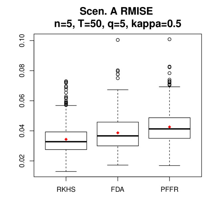
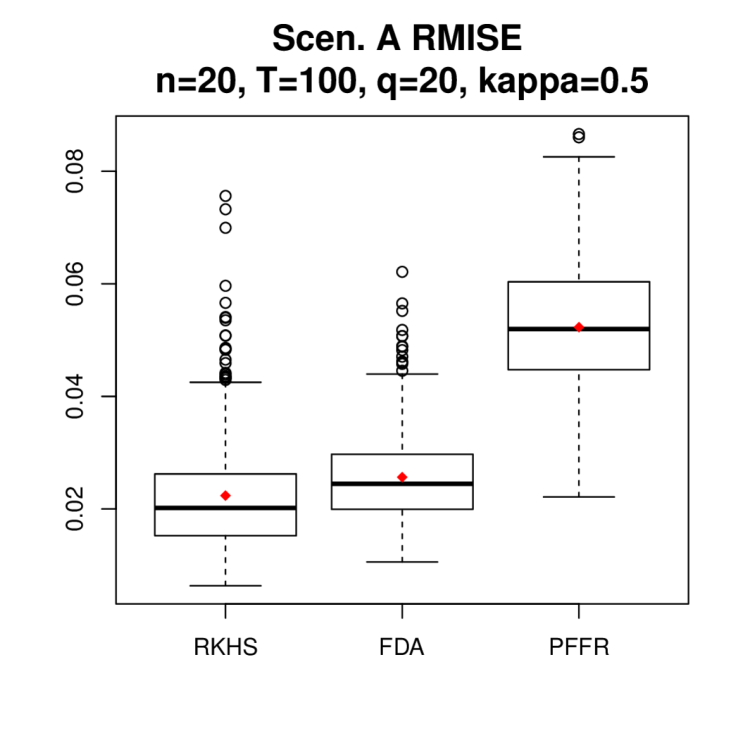
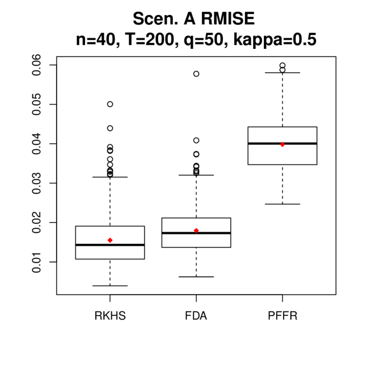
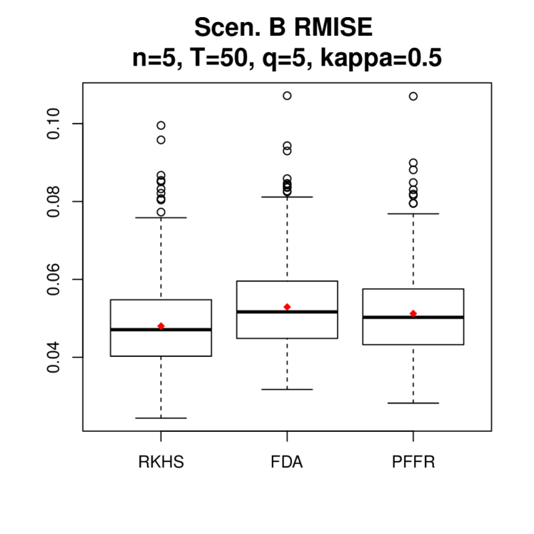
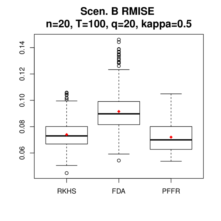
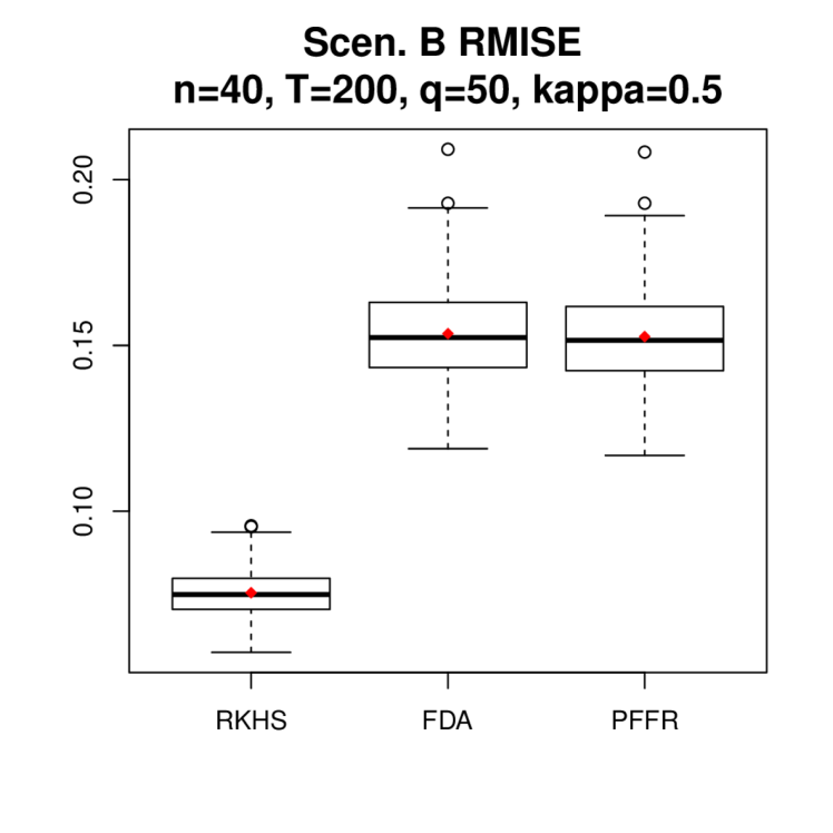
Figure 7: Boxplot of RMISE of RKHS, FDA and PFFR across 500 experiments under function-on-function regression with $\kappa=0.5$. Red points denote the average RMISE.

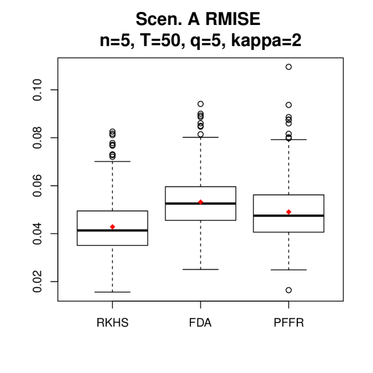
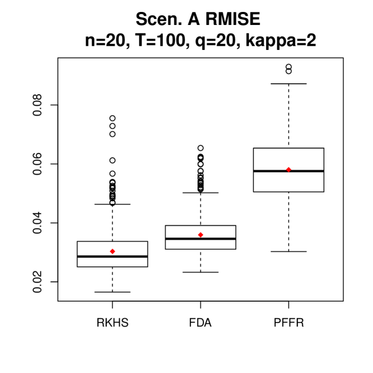
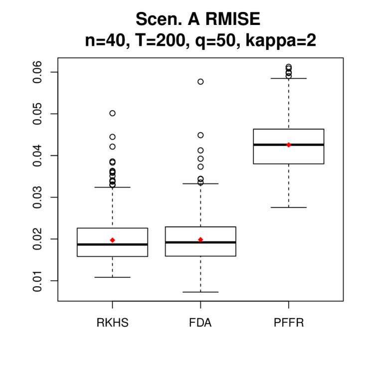
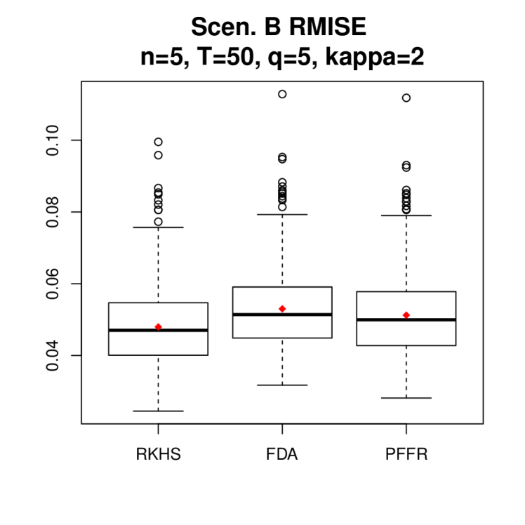
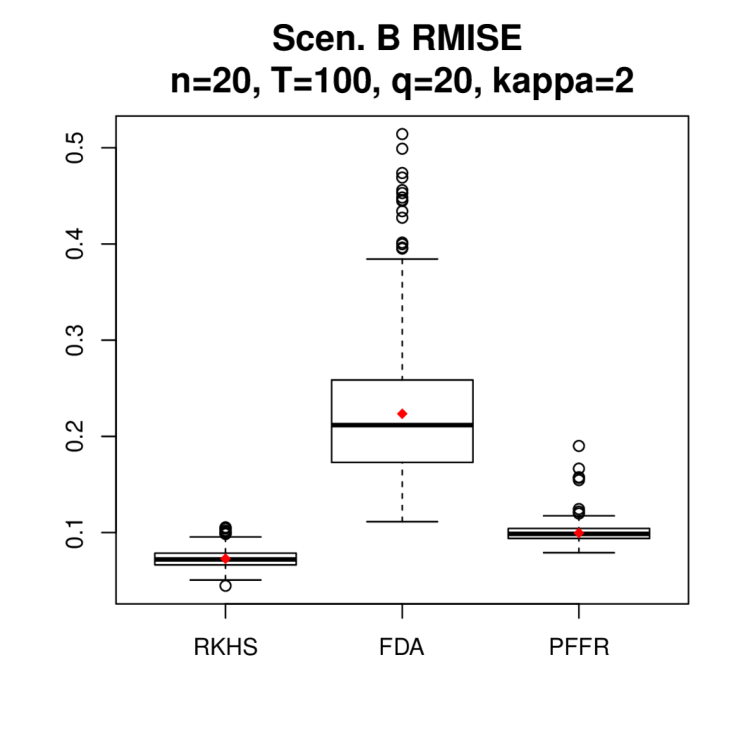
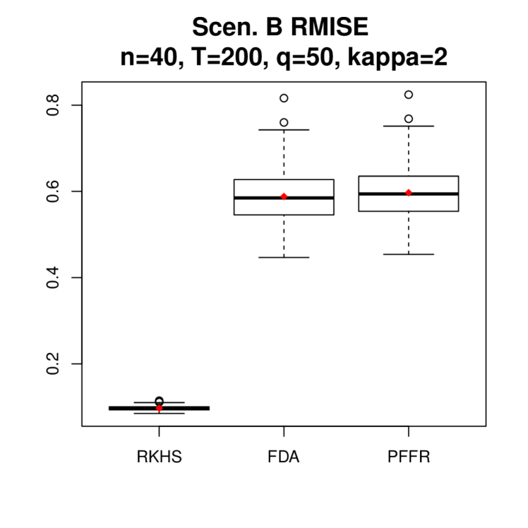
Figure 8: Boxplot of RMISE of RKHS, FDA and PFFR across 500 experiments under function-on-function regression with $\kappa=2$. Red points denote the average RMISE.

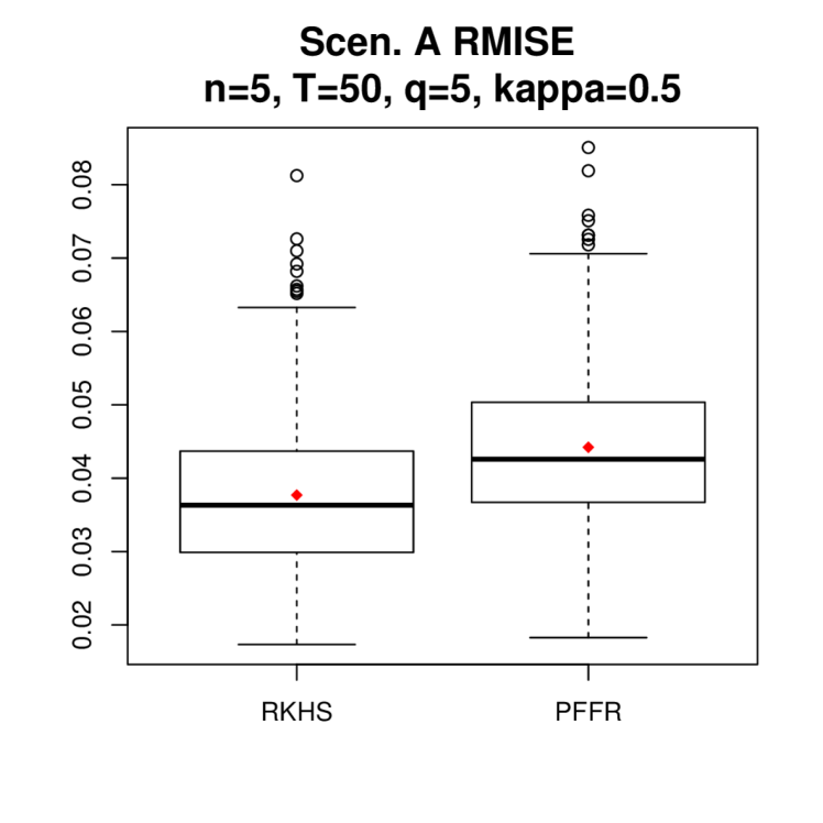
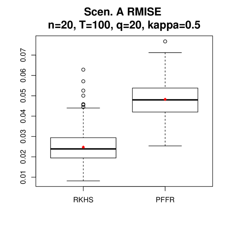
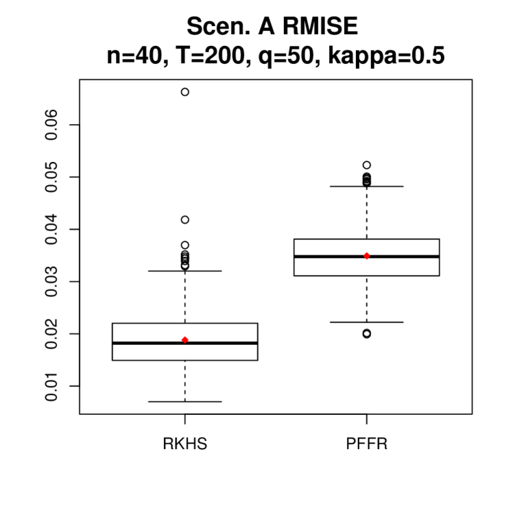
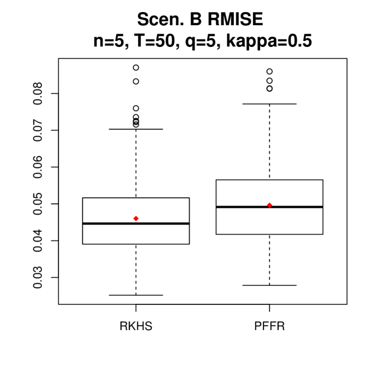
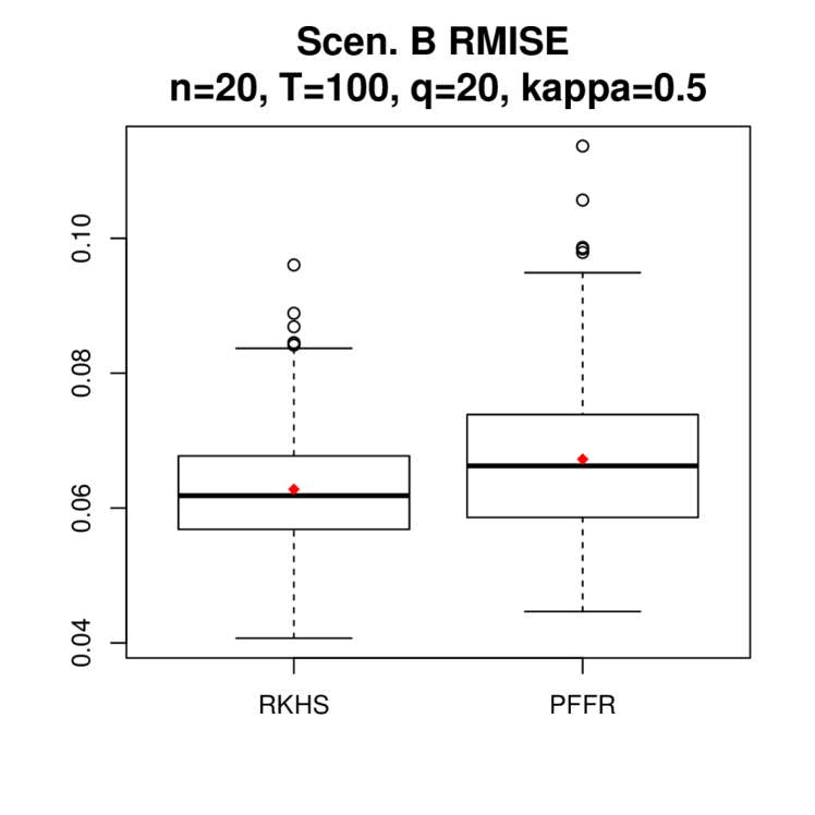
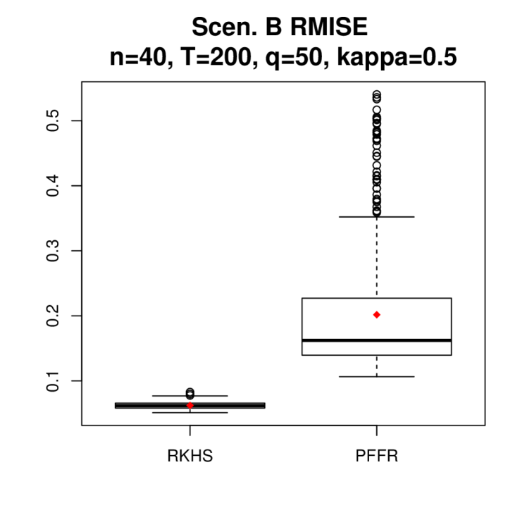
Figure 9: Boxplot of RMISE of RKHS and PFFR across 500 experiments under mixed functional regression with $\kappa=0.5$. Red points denote the average RMISE.

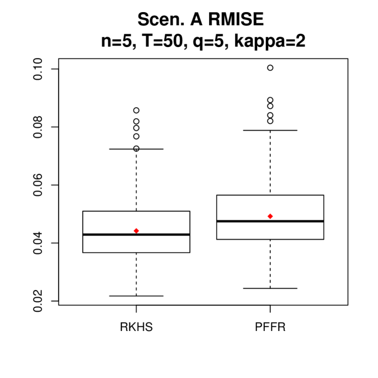
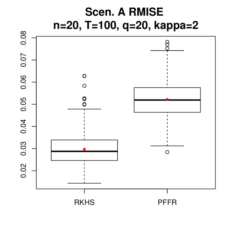
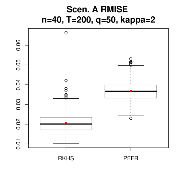
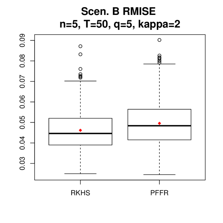
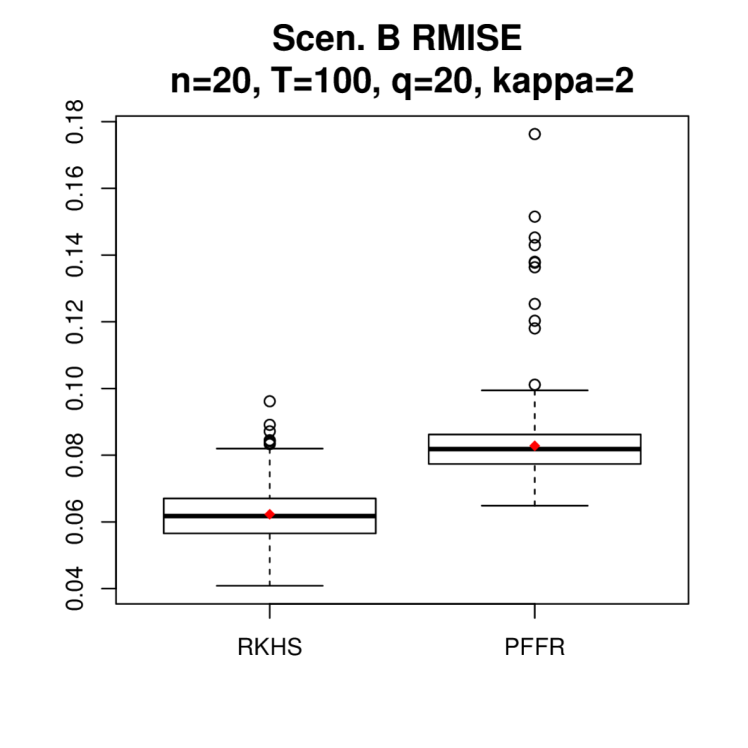
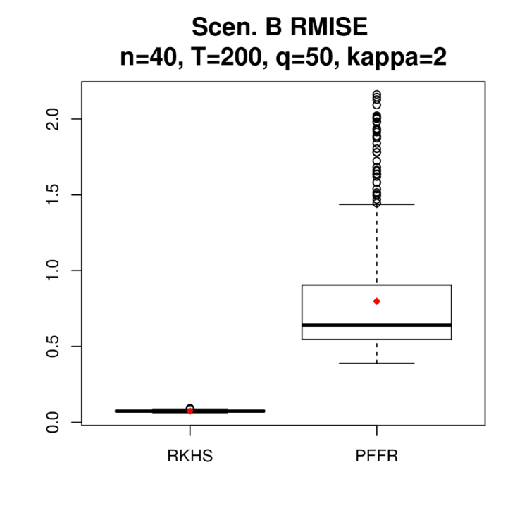
Figure 10: Boxplot of RMISE of RKHS and PFFR across 500 experiments under mixed functional regression with $\kappa=2$. Red points denote the average RMISE.

H Robustness check for real data analysis

In this section, we further provide a robustness check for the real data analysis presented in Section 5.4. Specifically, we repeat the two-fold CV procedure in Section 5.4 independently for 100 times for RKHS, FDA and PFFR. In addition, we also implement FDA with 50 basis functions (FDA50) and PFFR with 30 basis functions (PFFR30). We further compare with the popular functional PCA based regression method (FPCA) proposed in Yao et al. (2005).

Thus, for every method (RKHS, FDA, PFFR, FPCA), on each prediction day $s\in\{7,8,9,\cdots,20\}$, we have 100 RMSE_s and 100 MAE_s obtained from the 100 times two-fold CV. We refer to Section 5.4 for more detailed definition of RMSE and MAE.

Figure 12 visualizes the average RMSE_s and MAE_s over the 100 times CV achieved by different functional regression methods across $s\in\{7,8,9,\cdots,20\}$. As can be seen clearly, the pattern exhibited in Figure 12 is the same as the one in Figure 5 in Section 5.4 and RKHS is the winner by a notable margin. Note that FDA20 and FDA50 give essentially the same performance, while PFFR30 indeed gives worse performance than PFFR20. This suggests that 20 basis dimension is sufficient for the current real data application.

Table 3 further gives the number of two-fold CV (out of 100 times) where RKHS achieves the smallest RMSE_s and MAE_s for each $s\in\{7,8,9,\cdots,20\}$. As can be seen, RKHS is almost always the winner for every $s\in\{7,8,9,\cdots,20\}$ except for $s=19$, where RKHS still provides the best performance more than two thirds of the time.

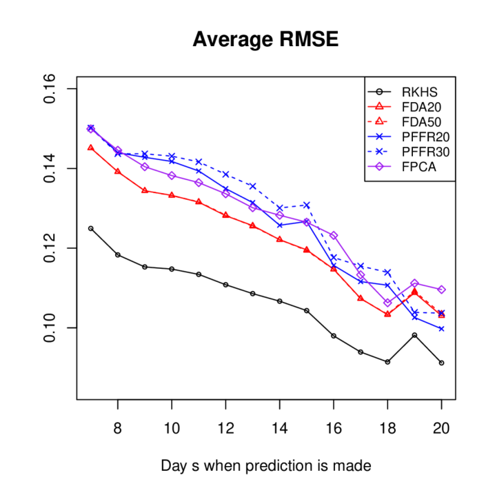
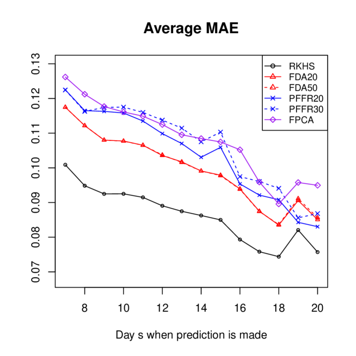
Figure 12: RMSE_s and MAE_s achieved by different functional regression methods averaged over 100 two-fold cross-validations for each $s\in\{7,8,9,\cdots,20\}$.

$s$	7	8	9	10	11	12	13	14	15	16	17	18	19	20
RMSEs	100	100	100	100	100	100	100	100	100	100	100	100	77	97
MAEs	100	100	100	100	100	100	100	100	100	100	100	100	66	96

Table 3: Number of two-fold cross-validations (out of 100 times) where RKHS achieves the smallest RMSE_s and MAE_s for each $s\in\{7,8,9,\cdots,20\}$.

I Numerical results for observations with measurement error

In this section, we conduct simulation experiments to examine the performance of different methods, including FDA, PFFR and the proposed RKHS, under the setting where the observed functional responses are additionally corrupted with measurement error.

The simulation analysis is done under the function-on-function regression setting as in Section 5.2. Specifically, for the ease of comparison, we use exactly the same simulation setting that generates Table 1 in Section 5.2. The only difference is that we assume we do not observe the functional response $Y_{t}(r_{j})$ directly but instead a noisy version of it, denoted by $y_{tj}$, corrupted with measurement error such that

$$y_{tj}=Y_{t}(r_{j})+\mathfrak{E}_{tj},$$

where $\mathfrak{E}_{tj}$ are independent Gaussian random variable with mean 0 and variance $\sigma^{2}_{\mathfrak{E}}$ for $t=1,\ldots,T$ and $j=1,\ldots,n_{2}.$ Note that for $\sigma^{2}_{\mathfrak{E}}=0$, we get back to the identical setting as in Section 5.2. It is easy to derive that the overall variability of the functional noise (i.e. $\mathbb{E}\int_{[0,1]}\epsilon_{t}(r)^{2}\,\mathrm{d}r$) under the simulation setting in Section 5.2 is around $0.4^{2}/12\approx 0.115^{2}$, which can be calculated easily using the fact that $\epsilon_{t}(r)=\sum_{i=1}^{q}e_{ti}u_{i}(r)$. We refer to Sections 5.1 and 5.2 for more details.

Thus, in the following, we set the variance of the measurement error as $\sigma^{2}_{\mathfrak{E}}=0.12^{2}$ such that the variability of the functional noise and the measurement error are comparable. For each setting, we conduct 500 experiments. We again use RMISE to evaluate the excess risk of each estimator. Due to limited space, we only report the result for the case where the spectral norm $\kappa=1$. The results for $\kappa=0.5$ and $\kappa=2$ are similar and omitted.

For each method, Table 4 reports its average nRMISE across 500 experiments under all simulation settings. Note that Table 4 is directly comparable with Table 1 in Section 5.2 (for $\kappa=1$), which reports the performance of each method for $\sigma_{\mathfrak{E}}^{2}=0.$ Thus, for ease of comparison, we copy the result reported in Table 1 (for $\kappa=1$) to Table 4 under the name $\sigma_{\mathfrak{E}}^{2}=0$.

Examining Table 4, it can be seen clearly that, compared to the case of no measurement error (i.e. $\sigma^{2}_{\mathfrak{E}}=0$), the performance of all three estimators (RKHS, FDA and PFFR) only worsen slightly when the variability of the measurement error and functional noise are comparable (i.e. $\sigma^{2}_{\mathfrak{E}}=0.12^{2}$), suggesting that functional noise is more difficult to handle than the independent measurement error. This can also be viewed as numerical support for the result in Theorem 4, i.e. the convergence rate of RKHS is not affected when the functional response is corrupted by independent mean zero measurement errors with a bounded variance.

	Scenario A: $n=5,T=50,q=5$					Scenario B: $n=5,T=50,q=5$
$\sigma_{\mathfrak{E}}^{2}$	RKHS	FDA	PFFR	Ravg(%)	Rw (%)	RKHS	FDA	PFFR	Ravg(%)	Rw (%)
$0$	9.14	10.31	10.98	12.81	68	10.42	11.50	11.12	6.63	71
$0.12^{2}$	10.14	11.40	12.20	12.45	64	12.61	13.87	13.23	4.96	64
	Scenario A: $n=20,T=100,q=20$					Scenario B: $n=20,T=100,q=20$
$\sigma^{2}_{\mathfrak{E}}$	RKHS	FDA	PFFR	Ravg(%)	Rw (%)	RKHS	FDA	PFFR	Ravg(%)	Rw (%)
$0$	5.89	6.75	12.84	14.66	81	18.39	32.41	22.32	21.37	92
$0.12^{2}$	5.87	6.86	12.44	16.93	84	22.09	34.67	25.22	14.17	83
	Scenario A: $n=40,T=200,q=50$					Scenario B: $n=40,T=200,q=50$
$\sigma^{2}_{\mathfrak{E}}$	RKHS	FDA	PFFR	Ravg(%)	Rw (%)	RKHS	FDA	PFFR	Ravg(%)	Rw (%)
$0$	3.98	4.41	9.68	10.96	75	20.75	76.74	77.40	269.73	100
$0.12^{2}$	4.02	4.47	9.75	11.32	77	23.71	76.95	77.52	224.49	100

Table 4: Numerical performance of RKHS, FDA and PFFR under function-on-function regression with no measurement error ($\sigma^{2}_{\mathfrak{E}}=0$) and with measurement error ($\sigma^{2}_{\mathfrak{E}}=0.12^{2}$). The reported nRMISE_avg is multiplied by 100 in scale. R_avg reflects the percent improvement of RKHS over the best performing competitor, and R_w reflects the percentage of experiments in which RKHS achieves the lowest RMISE.

J FDA and PFFR with larger number of basis functions

As discussed in Section 5.2, the performance of the penalized basis function approaches, such as FDA and PFFR, may be sensitive to the hyper-parameter $N_{b}$, which is the number of basis dimension used in the estimation.

In this section, we further examine the performance of FDA and PFFR with a larger $N_{b}.$ Specifically, we use the identical simulation setting as that in Section 5.2. We keep the implementation of RKHS the same and the only difference is that we implement FDA with $N_{b}=50$ and PFFR with $N_{b}=30$ instead of $N_{b}=20$. (For PFFR we can only do $N_{b}=30$ as the computational cost of PFFR with $N_{b}>30$ is practically forbidden for large-scale comparison. See later for more details.)

For each method, Table 5 reports the average nRMISE (nRMISE_avg) across 500 experiments under all simulation settings. Table 5 is directly comparable with Table 1 in Section 5.2. Cross-examining Table 5 and Table 1, we have the following observations. For Scenario A, where the bivariate function $A^{*}(r,s)$ is a simple exponential function, FDA50 and PFFR30 give essentially the same performance as $N_{b}=20$. The same applies to Scenario B with $q=5$ and with $q=20$ (for low SNR parameter $\kappa=0.5$). This indicates that $N_{b}=20$ is sufficient for simulation settings with low model complexity. On the other hand, for Scenario B with $q=20$ (for high SNR parameter $\kappa=1,2$) and $q=50$, compared to $N_{b}=20$, FDA50 and PFFR30 give much improved performance due to lower approximation bias, though still having a notable performance gap compared to RKHS. We further give the boxplot of RMISE for each method in Figure 13 under $\kappa=1$. The general pattern is the same as that exhibited in Figure 2 for $N_{b}=20$, where RKHS provides the best overall performance.

	Scenario A: $n=5,T=50,q=5$					Scenario B: $n=5,T=50,q=5$
$\kappa$	RKHS	FDA50	PFFR30	Ravg(%)	Rw (%)	RKHS	FDA50	PFFR30	Ravg(%)	Rw (%)
$0.5$	15.98	17.98	19.77	12.41	64	20.86	22.97	22.30	6.88	64
$1$	9.14	10.32	10.97	12.74	68	10.42	11.51	11.12	6.66	71
$2$	4.99	6.17	5.69	14.22	72	5.21	5.75	5.55	6.69	74
	Scenario A: $n=20,T=100,q=20$					Scenario B: $n=20,T=100,q=20$
$\kappa$	RKHS	FDA50	PFFR30	Ravg(%)	Rw (%)	RKHS	FDA50	PFFR30	Ravg(%)	Rw (%)
$0.5$	10.61	11.94	25.93	12.55	77	37.41	40.65	40.53	8.34	58
$1$	5.89	6.77	13.32	14.96	81	18.39	20.63	19.75	7.43	73
$2$	3.60	3.89	6.98	7.99	72	9.19	11.75	9.98	8.52	87
	Scenario A: $n=40,T=200,q=50$					Scenario B: $n=40,T=200,q=50$
$\kappa$	RKHS	FDA50	PFFR30	Ravg(%)	Rw (%)	RKHS	FDA50	PFFR30	Ravg(%)	Rw (%)
$0.5$	7.37	8.54	21.00	15.86	82	39.22	48.27	72.42	23.40	94
$1$	3.98	4.40	10.70	10.75	75	20.75	35.82	70.61	76.05	100
$2$	2.34	2.34	5.57	0.11	47	12.59	29.77	70.20	151.92	100

Table 5: Numerical performance of RKHS, FDA and PFFR under function-on-function regression. The reported nRMISE_avg is multiplied by 100 in scale. R_avg reflects the percent improvement of RKHS over the best performing competitor, and R_w reflects the percentage of experiments in which RKHS achieves the lowest RMISE.

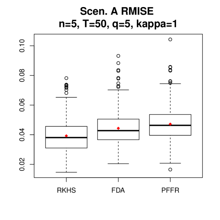
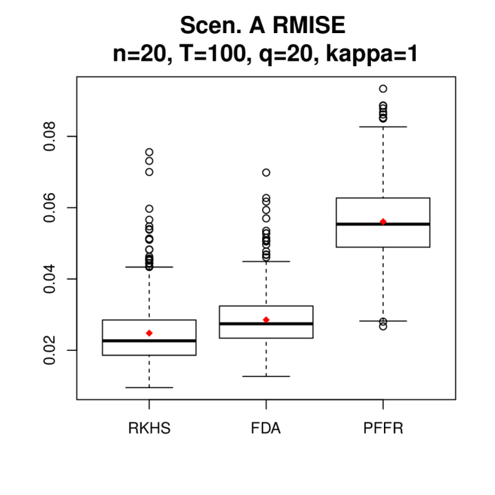
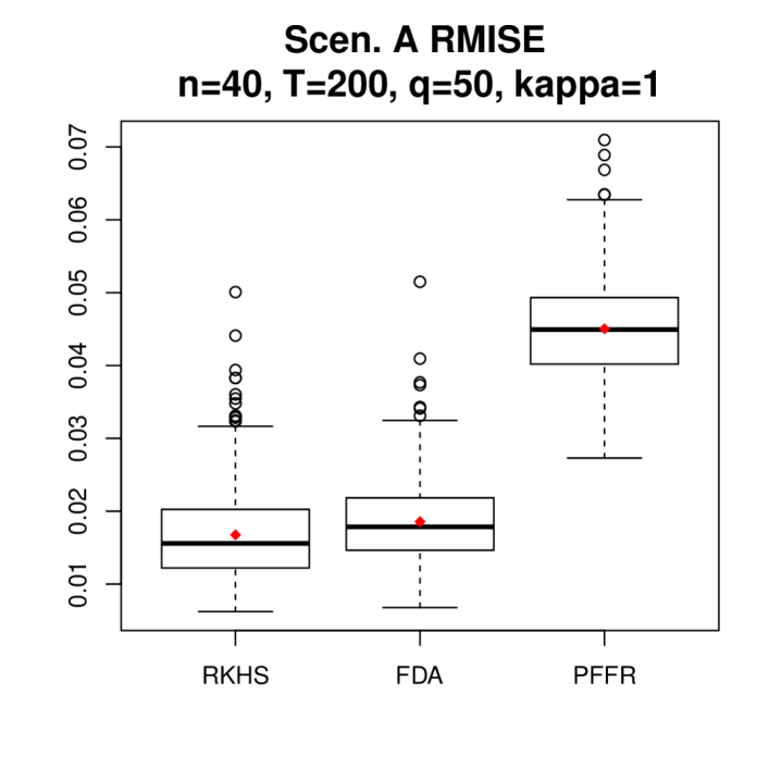
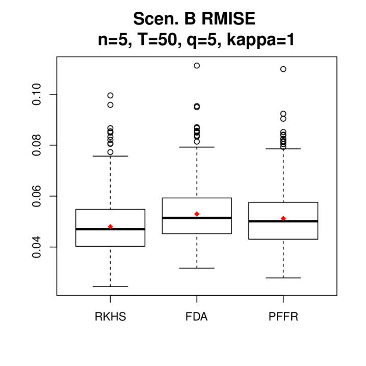
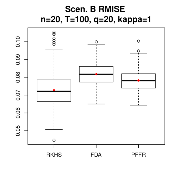
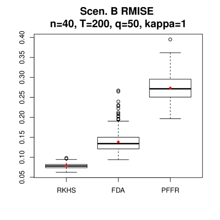
Figure 13: Boxplots of RMISE of RKHS, FDA50 and PFFR30 across 500 experiments under function-on-function regression with $\kappa=1$. Red points denote the average RMISE.

Computational Time: Note that a larger $N_{b}$ can significantly increase the computational cost of the penalized basis function approaches. For example, for FDA with the same number of basis functions $N_{b}$ for the first and second argument of the bivariate coefficient function $A(r,s)$, the computation of FDA involves inversion of an $N_{b}^{2}\times N_{b}^{2}$-dimension matrix (see equations (16.14) and (16.15) in Ramsay and Silverman (2005) for more details), which may not scale well with the number of basis $N_{b}$. PFFR uses restricted MLE (REML) for its model estimation by recasting the functional regression model as a penalized additive model with mixed effects (see Ivanescu et al. (2015) for more details), which seems to be slow in terms of computation and also does not scale well with $N_{b}$.

For illustration, Figure 14 gives the boxplot of computational time (in log-scale) for RKHS, FDA20, FDA50 with a fixed tuning parameter $(\lambda=10^{-15})$ and for PFFR20 and PFFR30 across 500 experiments. To conserve space, we present the case for Scenario B with $\kappa=1.$ Results under other settings are similar and thus omitted. Note that for FDA and RKHS, the computational time does not depend on $\lambda$ as we have closed-form solutions. For PFFR, it uses REML to automatically select the roughness penalty and does not require cross-validation. Thus, for fair comparison, if RKHS and FDA requires a 5-fold cross-validation to search for the best tuning parameters among 50 candidates, we need to add $\log(250)\approx 4.6$ to the log time for FDA and RKHS on Figure 14.

As can be seen from Figure 14, FDA50 incurs much higher computational cost compared to FDA20. Similarly, PFFR30 has noticeably higher computational cost than PFFR20. For the current simulation settings, RKHS has the lowest computational cost.

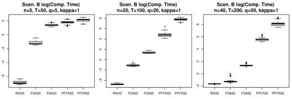
Figure 14: Boxplots of computational time (in log-scale) for RKHS, FDA20, FDA50 with a fixed tuning parameter $(\lambda=10^{-15})$ and for PFFR20 and PFFR30 across 500 experiments.

K Additional numerical comparison with FPCA

In this section, we further provide numerical comparison with the popular functional PCA based regression method (FPCA) proposed in Yao et al. (2005), which estimates the functional linear model based on Karhunen–Loéve expansion. FPCA is implemented via the Matlab package PACE (FPCreg function). We keep all tuning parameters as default values suggested in the PACE package.

Function-on-function regression: We first consider the function-on-function regression setting as in Section 5.2 of the main text. Specifically, we use the identical simulation setting that generates Figure 2 in Section 5.2. The only difference is that besides RKHS, FDA and PFFR, we further implement FPCA in the simulation.

For each setting, we conduct 500 experiments. We again use RMISE to evaluate the excess risk of each estimator. Due to limited space, we only report the result for the case where the spectral norm $\kappa=1$. The results for $\kappa=0.5$ and $\kappa=2$ are similar and omitted. For each method (RKHS, FDA, PFFR and FPCA), Figure 15 visualizes the boxplot of its RMISE across 500 experiments under each simulation setting. Note that the only different between Figure 2 and Figure 15 is that Figure 15 further includes the boxplot of RMISE for FPCA.

As can be seen, for Scenario A, where the coefficient function $A(s,t)$ is the simple exponential function, FPCA provides reasonable performance. However, its performance is not satisfactory when the coefficient function $A(s,t)$ becomes more complex as in Scenario B. This phenomenon is well-known in the literature as the functional space spanned by the eigenfunctions associated with the leading principle components may not be able to well approximate the coefficient function $A(s,t)$, see Cai and Yuan (2012) and Sun et al. (2018) for similar observations.

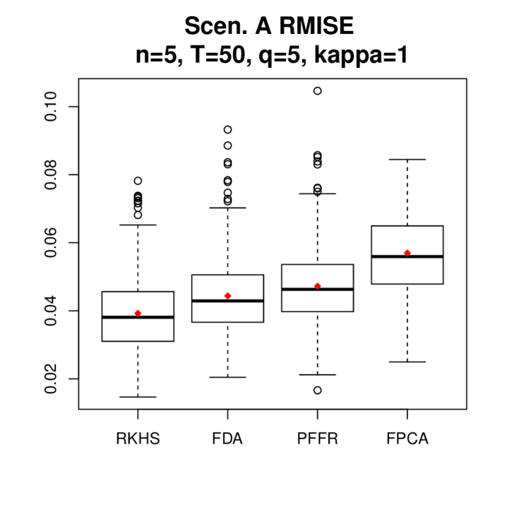
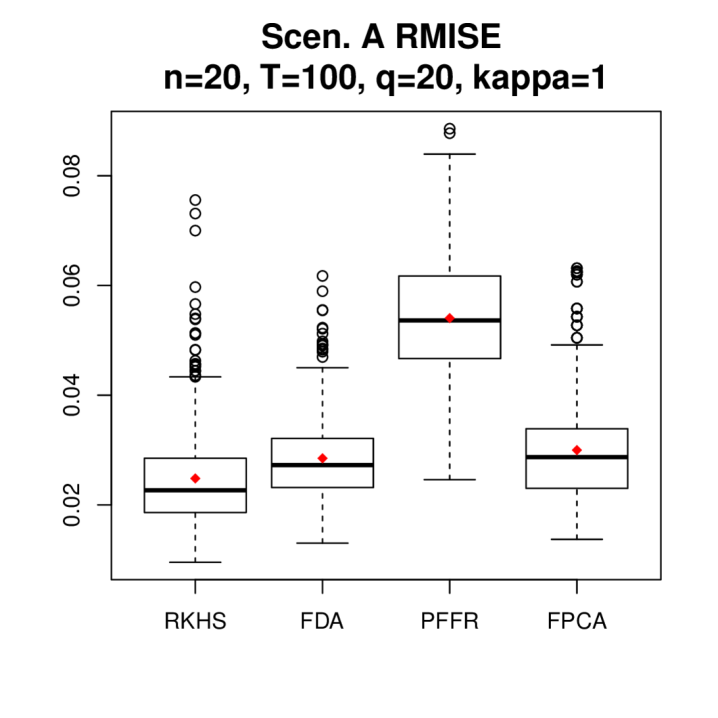
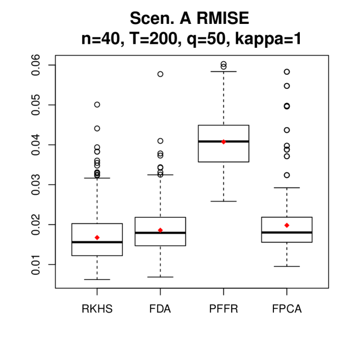
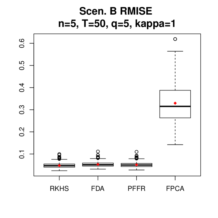
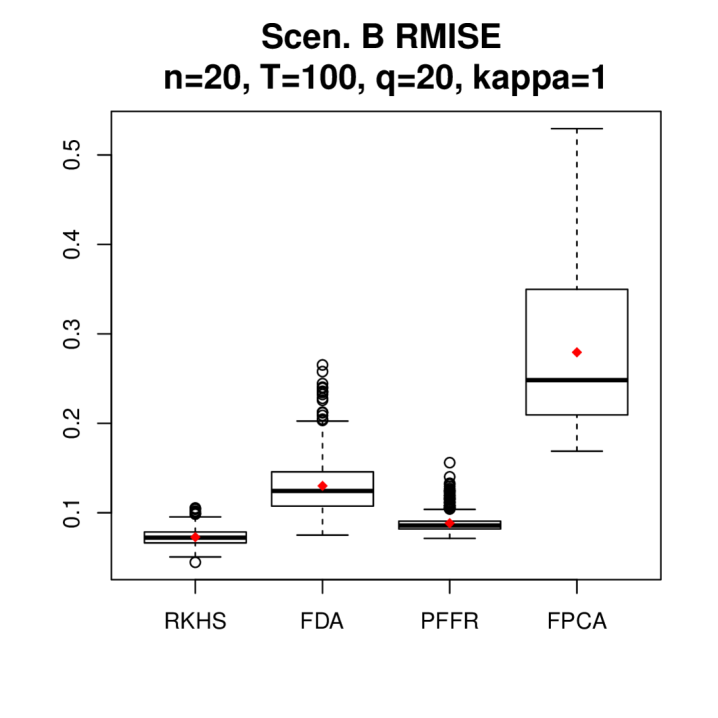
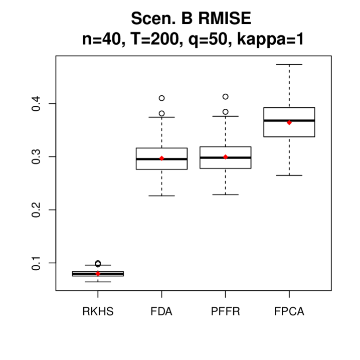
Figure 15: Boxplots of RMISE of RKHS, FDA, PFFR and FPCA across 500 experiments under function-on-function regression with $\kappa=1$. Red points denote the average RMISE.

Functional regression with mixed predictors: We then consider the functional regression with mixed covariates setting as in Section 5.3 of the main text. Specifically, we use the identical simulation setting that generates Figure 3 in Section 5.3. The only difference is that besides RKHS and PFFR, we further implement FPCA in the simulation.

Note that the original FPCreg function in the Matlab package PACE only supports function-on-function regression and does not support the general setting of functional regression with mixed covariates. Thus, we modify the original code in FPCreg to implement FPCA for functional regression with mixed covariates. The modification is straightforward, where we further include the observed scalar predictors $(Z_{t1},Z_{t2},Z_{t3})$ together with the estimated FPCs of the functional predictor $X_{t}$ to predict the FPCs of the functional response $Y_{t}.$

For each setting, we conduct 500 experiments. We again use RMISE to evaluate the excess risk of each estimator. Due to limited space, we only report the result for the case where the spectral norm $\kappa=1$. The results for $\kappa=0.5$ and $\kappa=2$ are similar and omitted. For each method (RKHS, PFFR and FPCA), Figure 16 visualizes the boxplot of its RMISE across 500 experiments under each simulation setting. Note that the only different between Figure 3 and Figure 16 is that Figure 16 further includes the boxplot of RMISE for FPCA.

As can be seen, the phenomenon is essentially the same as the one observed under the function-on-function regression setting. Specifically, for Scenario A, where the coefficient function $A(s,t)$ is the simple exponential function, FPCA provides reasonable performance. However, its performance is not satisfactory when the coefficient function $A(s,t)$ becomes more complex as in Scenario B. Again, this phenomenon is due to the fact that the functional space spanned by the eigenfunctions associated with the leading principle components may not be able to well approximate the coefficient function $A(s,t)$, see Cai and Yuan (2012) and Sun et al. (2018) for similar observations.

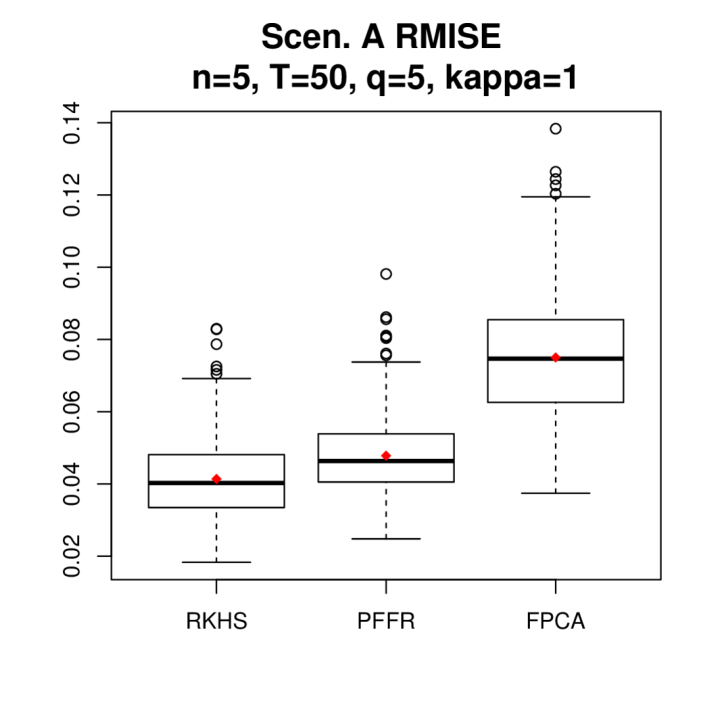
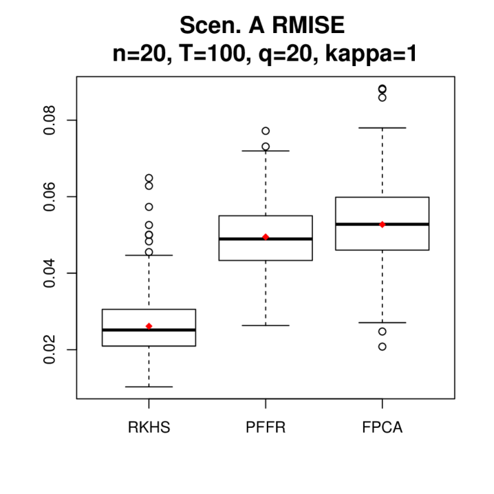
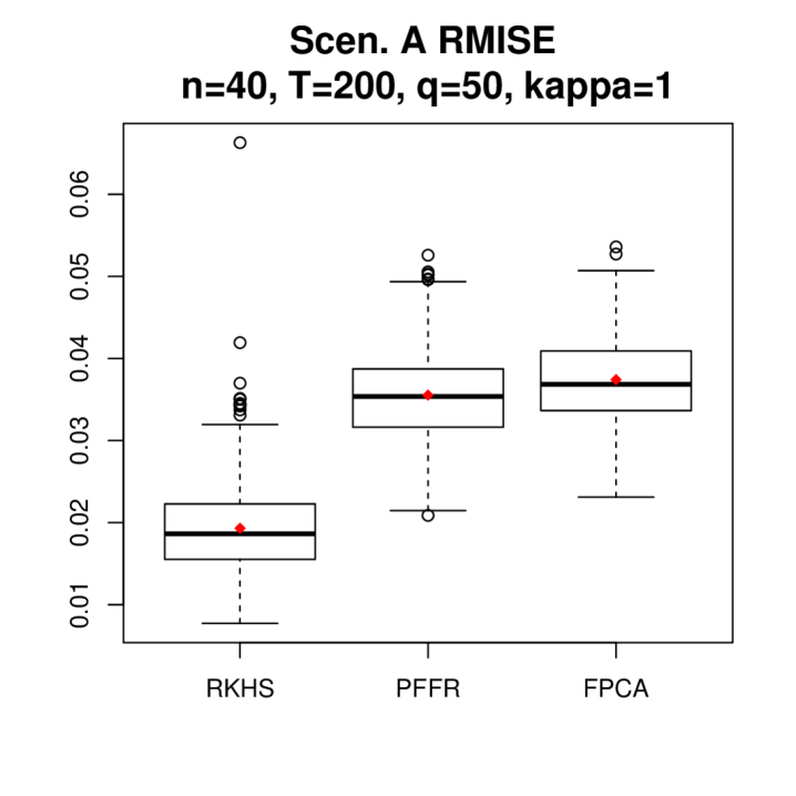
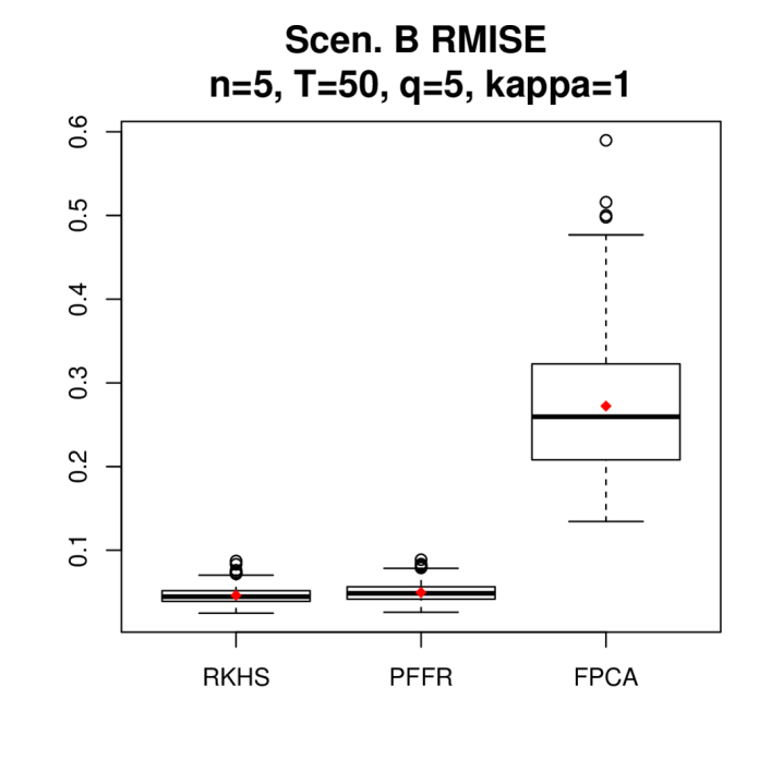
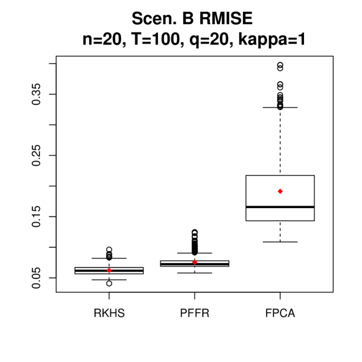
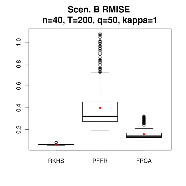
Figure 16: Boxplots of RMISE of RKHS, PFFR and FPCA across 500 experiments under functional regression with mixed predictors with $\kappa=1$. Red points denote the average RMISE.

L Illustration of phase transition

In this section, we provide an indirect numerical illustration for the phase transition phenomenon discovered in Theorem 2. Recall Theorem 2 suggests that putting aside the discretization error $\zeta_{n}$, there is a phase transition between a nonparametric rate $\delta_{T}$ and a high-dimensional parametric rate $\mathfrak{s}\log(p)/T$.

Here, the nonparametric rate $\delta_{T}$ takes the form $\delta_{T}=T^{-2r/(2r+1)}$ with some $r>1/2$ and is associated with the estimation of the bivariate coefficient function $A^{*}$. In other words, $\delta_{T}=T^{-c}$ for some $c>0$ and $c$ is strictly smaller than 1. The high-dimensional parametric rate $\mathfrak{s}\log(p)/T$ is associated with the estimation of the high-dimensional sparse univariate coefficient functions $\beta^{*}.$ In the following, we numerically verify these two rates by considering two special cases of the proposed functional linear model with mixed predictors.

Specifically, we follow the same simulation setting as Scenario B in Section 5.1 of the main text and simulate data from the functional linear regression model

$$Y_{t}(r)=\int_{[0,1]}A^{*}(r,s)X_{t}(s)\,\mathrm{d}s+\sum_{j=1}^{p}\beta^{*}_{j}(r)Z_{tj}+\epsilon_{t}(r),~{}r\in[0,1].$$ (87)

The functional predictor $X_{t}$, scalar predictor $Z_{t}$ and the functional error $\epsilon_{t}$ are generated using the same setting in Section 5.1. Following Scenario B, the coefficient functions $A^{*}$ and $\beta_{1}^{*},\ldots,\beta_{p}^{*}$ are generated from a $q$-dimensional subspace spanned by basis functions $\{u_{i}(s)\}_{i=1}^{q}$. We refer to Section 5.1 for more detailed description of Scenario B.

In the following, we fix the dimension $q=20$ and the SNR parameter $\kappa=2$. To minimize the impact of the discretization error $\zeta_{n}$, we set the discrete sample points $\{r_{j}\}_{j=1}^{n_{2}}$ for $Y_{t}$ and $\{s_{i}\}_{i=1}^{n_{1}}$ for $X_{t}$ to be evenly spaced dense grids on $[0,1]$ with a large number of grids $n=n_{1}=n_{2}=50$.

To evaluate the excess risk given by the RKHS estimator, we follow Section 5.1 and use the RMISE defined in (21). To match the result in Theorem 2, we compute MISE, which is the squared RMISE with MISE = RMISE².

Nonparametric rate $\delta_{T}$: We first focus on the nonparametric rate $\delta_{T}$ and consider the special case of (87) by setting $p=0$, i.e. the function-on-function regression. We vary the sample size $T=100,200,300,\ldots,2000$ and for each $T$ we conduct 500 experiments. For each sample size $T$, we compute the average MISE across the 500 experiments and Figure 17(A) gives the plot between $\log(\text{average MISE})$ and $\log(T)$, where the relationship is seen to be roughly linear. We further fit an ordinary least squared estimator (OLS) on the points, which gives an estimated slope of $-0.811$, confirming that $\delta_{T}$ takes the nonparametric rate $O(T^{-c})$ with $c$ being a positive constant less than 1.

High-dimensional parametric rate $\mathfrak{s}\log(p)/T$: We now focus on the high-dimensional parametric rate and consider the special case of (87) by setting $A^{*}=0$, i.e. we consider the functional linear regression with only scalar predictors $Z_{t1},Z_{t2},\cdots,Z_{tp}$.

We first fix $\mathfrak{s}=1$ and $T=200$, and vary the dimension $p=10,50,100,150,\ldots,450,500.$ In other words, the coefficient functions $\beta_{j}^{*}\equiv 0$ for $j=2,3,\ldots,p$ and $\beta_{1}^{*}$ is generated as in Scenario B of Section 5.1 (see more detailed description above). For each dimension $p$, we conduct 500 experiments and compute the average MISE. Figure 17(B) gives the plot between average MISE and $\log(p)$, where the relationship is seen to be roughly linear. This confirms that fixing the sparsity $\mathfrak{s}$ and sample size $T$, the excess risk increases in the order of $O\big{(}\log(p)\big{)}.$

We next fix $\mathfrak{s}=1$, $p=10$, and vary the sample size $T=100,200,300,\ldots,2000$. For each sample size $T$, we conduct 500 experiments and compute the average MISE. Figure 17(C) gives the plot between $\log(\text{average MISE})$ and $\log(T)$, where the relationship is seen to be roughly linear. We further fit an OLS on the points, which gives an estimated slope of $-1.012$, confirming that fixing the sparsity $\mathfrak{s}$ and dimension $p$, the excess risk decreases in the order of roughly $O(1/T).$

Finally, we fix $T=200$, $p=100$, and vary the sparsity $\mathfrak{s}=1,2,5,10,15,20.$ In other words, the coefficient functions $\beta_{j}^{*}\equiv 0$ for $j=\mathfrak{s}+1,\mathfrak{s}+2,\ldots,p$ and $\beta_{1}^{*}=\beta_{2}^{*}=\cdots=\beta_{\mathfrak{s}}^{*}$ are generated as in Scenario B of Section 5.1. For each sparsity $\mathfrak{s}$, we conduct 500 experiments and compute the average MISE. Figure 17(D) gives the plot between $\log(\text{average MISE})$ and $\log(\mathfrak{s})$, where the relationship is seen to be roughly linear. We further fit an OLS on the points, which gives an estimated slope of $1.087$, confirming that fixing the sample size $T$ and dimension $p$, the excess risk increases in the order of roughly $O(\mathfrak{s}).$

Thus, we numerically illustrate that the prediction error associated with the estimation of the high-dimensional sparse univariate coefficient functions $\beta^{*}$ is of order $O\big{(}\mathfrak{s}\log(p)/T\big{)}$. Putting these two cases together, we can conclude that there is a phase transition phenomenon between a nonparametric rate $O(T^{-c})$ and a high-dimensional parametric rate $O\big{(}\mathfrak{s}\log(p)/T\big{)}$.

Figure 17: Numerical illustration of the nonparametric rate (A) and the high-dimensional parametric rate (B-D).

References

- Aue et al. (2015) Alexander Aue, Diogo Dubart Norinho, and Siegfried Hörmann. On the prediction of stationary functional time series. Journal of the American Statistical Association, 110(509):378–392, 2015.
- Bartlett et al. (2005) Peter L Bartlett, Olivier Bousquet, and Shahar Mendelson. Local rademacher complexities. The Annals of Statistics, 33(4):1497–1537, 2005.
- Bathia et al. (2010) Neil Bathia, Qiwei Yao, and Flavio Ziegelmann. Identifying the finite dimensionality of curve time series. The Annals of Statistics, 38(6):3352–3386, 2010.
- Benko (2007) Michal Benko. Functional data analysis with applications in finance. Humboldt-Universität zu Berlin, Wirtschaftswissenschaftliche Fakultät, 2007.
- Bonner et al. (2014) Simon J Bonner, Nathaniel K Newlands, and Nancy E Heckman. Modeling regional impacts of climate teleconnections using functional data analysis. Environmental and ecological statistics, 21(1):1–26, 2014.
- Brezis (2010) Haim Brezis. Functional analysis, Sobolev spaces and partial differential equations. Springer Science & Business Media, 2010.
- Bühlmann and van de Geer (2011) Peter Bühlmann and Sara van de Geer. Statistics for high-dimensional data: methods, theory and applications. Springer Science & Business Media, 2011.
- Cai and Hall (2006) T Tony Cai and Peter Hall. Prediction in functional linear regression. The Annals of Statistics, 34(5):2159–2179, 2006.
- Cai and Yuan (2011) T Tony Cai and Ming Yuan. Optimal estimation of the mean function based on discretely sampled functional data: Phase transition. The annals of statistics, 39(5):2330–2355, 2011.
- Cai and Yuan (2012) T Tony Cai and Ming Yuan. Minimax and adaptive prediction for functional linear regression. Journal of the American Statistical Association, 107(499):1201–1216, 2012.
- Cai and Yuan (2010) Tony Cai and Ming Yuan. Nonparametric covariance function estimation for functional and longitudinal data. University of Pennsylvania and Georgia inistitute of technology, 2010.
- Cardot et al. (2003) Hervé Cardot, Frédéric Ferraty, and Pascal Sarda. Spline estimators for the functional linear model. Statistica Sinica, pages 571–591, 2003.
- Chen et al. (2017) Kehui Chen, Pedro Francisco Delicado Useros, and Hans-Georg Müller. Modelling function-valued stochastic processes, with applications to fertility dynamics. Journal of the Royal Statistical Society. Series B, Statistical Methodology, 79(1):177–196, 2017.
- Chiou et al. (2014) Jeng-Min Chiou, Yi-Chen Zhang, Wan-Hui Chen, and Chiung-Wen Chang. A functional data approach to missing value imputation and outlier detection for traffic flow data. Transportmetrica B: Transport Dynamics, 2(2):106–129, 2014.
- Dai et al. (2019) Xiongtao Dai, Hans-Georg Müller, Jane-Ling Wang, and Sean CL Deoni. Age-dynamic networks and functional correlation for early white matter myelination. Brain Structure and Function, 224(2):535–551, 2019.
- Evans (2010) Lawrence C Evans. Partial differential equations. second. vol. 19. Graduate Studies in Mathematics. American Mathematical Society, 2010.
- Fan et al. (2014) Yingying Fan, Natasha Foutz, Gareth M James, and Wolfgang Jank. Functional response additive model estimation with online virtual stock markets. The Annals of Applied Statistics, 8(4):2435–2460, 2014.
- Fan et al. (2015) Yingying Fan, Gareth M James, and Peter Radchenko. Functional additive regression. The Annals of Statistics, 43(5):2296–2325, 2015.
- Faraway (1997) Julian J Faraway. Regression analysis for a functional response. Technometrics, 39(3):254–261, 1997.
- Ferraty and Vieu (2009) Frédéric Ferraty and Philippe Vieu. Additive prediction and boosting for functional data. Computational Statistics & Data Analysis, 53(4):1400–1413, 2009.
- Fraiman et al. (2014) Ricardo Fraiman, Ana Justel, Regina Liu, and Pamela Llop. Detecting trends in time series of functional data: A study of antarctic climate change. Canadian Journal of Statistics, 42(4):597–609, 2014.
- Friedman et al. (2010) Jerome H. Friedman, Trevor Hastie, and Robert Tibshirani. A note on the group lasso and a sparse group lasso. arXiv:1001.0736, 2010.
- Gu (2013) Chong Gu. Smoothing Spline ANOVA Models. Springer-Verlag, New York, 2 edition, 2013.
- Hadjipantelis et al. (2015) Pantelis Z Hadjipantelis, John AD Aston, Hans-Georg Müller, and Jonathan P Evans. Unifying amplitude and phase analysis: A compositional data approach to functional multivariate mixed-effects modeling of mandarin chinese. Journal of the American Statistical Association, 110(510):545–559, 2015.
- Hall and Horowitz (2007) Peter Hall and Joel L Horowitz. Methodology and convergence rates for functional linear regression. The Annals of Statistics, 35(1):70–91, 2007.
- Hastie et al. (2009) Trevor Hastie, Robert Tibshirani, and Jerome H. Friedman. The Elements of Statistical Learning. Springer-Verlag New York, 2 edition, 2009.
- Ivanescu et al. (2015) Andrada E Ivanescu, Ana-Maria Staicu, Fabian Scheipl, and Sonja Greven. Penalized function-on-function regression. Computational Statistics, 30(2):539–568, 2015.
- Jiang et al. (2014) Ci-Ren Jiang, Wei Yu, Jane-Ling Wang, et al. Inverse regression for longitudinal data. The Annals of Statistics, 42(2):563–591, 2014.
- Kneip et al. (2016) Alois Kneip, Dominik Poß, and Pascal Sarda. Functional linear regression with points of impact. The Annals of Statistics, 44(1):1–30, 2016.
- Koltchinskii and Yuan (2010) Vladimir Koltchinskii and Ming Yuan. Sparsity in multiple kernel learning. The Annals of Statistics, 38(6):3660–3695, 2010.
- Laird and Ware (1982) Nan M Laird and James H Ware. Random-effects models for longitudinal data. Biometrics, pages 963–974, 1982.
- Li and Hsing (2010) Yehua Li and Tailen Hsing. Uniform convergence rates for nonparametric regression and principal component analysis in functional/longitudinal data. The Annals of Statistics, 38(6):3321–3351, 2010.
- Liang et al. (2003) Hua Liang, Hulin Wu, and Raymond J Carroll. The relationship between virologic and immunologic responses in aids clinical research using mixed-effects varying-coefficient models with measurement error. Biostatistics, 4(2):297–312, 2003.
- Lin and Yuan (2006) Yi Lin and Ming Yuan. Convergence rates of compactly supported radial basis function regularization. Statistica Sinica, pages 425–439, 2006.
- Loh and Wainwright (2012) Po-Ling Loh and Martin J Wainwright. High-dimensional regression with noisy and missing data: Provable guarantees with nonconvexity. The Annals of Statistics, 40(3):1637–1664, 2012.
- Mendelson (2002) Shahar Mendelson. Geometric parameters of kernel machines. In International Conference on Computational Learning Theory, pages 29–43. Springer, 2002.
- Mercer (1909) James Mercer. Xvi. functions of positive and negative type, and their connection the theory of integral equations. Philosophical transactions of the royal society of London. Series A, containing papers of a mathematical or physical character, 209(441-458):415–446, 1909.
- Morris (2015) Jeffrey S Morris. Functional regression. Annual Review of Statistics and Its Application, 2:321–359, 2015.
- Park et al. (2018) Byeong U Park, Chun-Jui Chen, Wenwen Tao, and Hans-Georg Müller. Singular additive models for function to function regression. Statistica Sinica, 28(4):2497–2520, 2018.
- Petersen et al. (2019) Alexander Petersen, Sean Deoni, and Hans-Georg Müller. Fréchet estimation of time-varying covariance matrices from sparse data, with application to the regional co-evolution of myelination in the developing brain. The Annals of Applied Statistics, 13(1):393–419, 2019.
- Ramsay and Ramsey (2002) James O Ramsay and James B Ramsey. Functional data analysis of the dynamics of the monthly index of nondurable goods production. Journal of Econometrics, 107(1-2):327–344, 2002.
- Ramsay and Silverman (2005) J.O. Ramsay and B.W. Silverman. Functional Data Analysis. Springer-Verlag, New York, 2005.
- Raskutti et al. (2010) Garvesh Raskutti, Martin J Wainwright, and Bin Yu. Restricted eigenvalue properties for correlated gaussian designs. The Journal of Machine Learning Research, 11:2241–2259, 2010.
- Raskutti et al. (2011) Garvesh Raskutti, Martin J Wainwright, and Bin Yu. Minimax rates of estimation for high-dimensional linear regression over lq -balls. IEEE transactions on information theory, 57(10):6976–6994, 2011.
- Raskutti et al. (2012) Garvesh Raskutti, Martin J Wainwright, and Bin Yu. Minimax-optimal rates for sparse additive models over kernel classes via convex programming. Journal of machine learning research, 13(2), 2012.
- Ratcliffe et al. (2002) Sarah J Ratcliffe, Gillian Z Heller, and Leo R Leader. Functional data analysis with application to periodically stimulated foetal heart rate data. ii: Functional logistic regression. Statistics in medicine, 21(8):1115–1127, 2002.
- Reimherr et al. (2018) Matthew Reimherr, Bharath Sriperumbudur, Bahaeddine Taoufik, et al. Optimal prediction for additive function-on-function regression. Electronic Journal of Statistics, 12(2):4571–4601, 2018.
- Reimherr et al. (2019) Matthew Reimherr, Bharath Sriperumbudur, and Hyun Bin Kang. Optimal function-on-scalar regression over complex domains. arXiv preprint arXiv:1902.07284, 2019.
- Sun et al. (2018) Xiaoxiao Sun, Pang Du, Xiao Wang, and Ping Ma. Optimal penalized function-on-function regression under a reproducing kernel hilbert space framework. Journal of the American Statistical Association, 113(524):1601–1611, 2018.
- Tavakoli et al. (2019) Shahin Tavakoli, Davide Pigoli, John AD Aston, and John S Coleman. A spatial modeling approach for linguistic object data: Analyzing dialect sound variations across great britain. Journal of the American Statistical Association, 114(527):1081–1096, 2019.
- Valencia and Yuan (2013) Carlos Valencia and Ming Yuan. Radial basis function regularization for linear inverse problems with random noise. Journal of Multivariate Analysis, 116:92–108, 2013.
- van Delft et al. (2017) Anne van Delft, Vaidotas Characiejus, and Holger Dette. A nonparametric test for stationarity in functional time series. arXiv preprint arXiv:1708.05248, 2017.
- Vershynin (2018) Roman Vershynin. High-dimensional probability: An introduction with applications in data science, volume 47. Cambridge university press, 2018.
- Wagner-Muns et al. (2017) Isaac Michael Wagner-Muns, Ivan G Guardiola, VA Samaranayke, and Wasim Irshad Kayani. A functional data analysis approach to traffic volume forecasting. IEEE Transactions on Intelligent Transportation Systems, 19(3):878–888, 2017.
- Wahba (1990) Grace Wahba. Spline models for observational data. SIAM, 1990.
- Wang et al. (2020a) Daren Wang, Zifeng Zhao, Rebecca Willett, and Chun Yip Yau. Functional autoregressive processes in reproducing kernel hilbert spaces. arXiv preprint arXiv:2011.13993, 2020a.
- Wang et al. (2016) Jane-Ling Wang, Jeng-Min Chiou, and Hans-Georg Müller. Functional data analysis. Annual Review of Statistics and Its Application, 3:257–295, 2016.
- Wang et al. (2020b) Jiayi Wang, Raymond KW Wong, and Xiaoke Zhang. Low-rank covariance function estimation for multidimensional functional data. Journal of the American Statistical Association, pages 1–14, 2020b.
- Wang et al. (2014) Yu-Xiang Wang, Alex Smola, and Ryan Tibshirani. The falling factorial basis and its statistical applications. In International Conference on Machine Learning, pages 730–738. PMLR, 2014.
- Wright (2015) Stephen J. Wright. Coordinate descent algorithms. Mathematical Programming, 151:3–34, 2015.
- Wu and Chiang (2000) Colin O Wu and Chin-Tsang Chiang. Kernel smoothing on varying coefficient models with longitudinal dependent variable. Statistica Sinica, pages 433–456, 2000.
- Wu et al. (1998) Colin O Wu, Chin-Tsang Chiang, and Donald R Hoover. Asymptotic confidence regions for kernel smoothing of a varying-coefficient model with longitudinal data. Journal of the American statistical Association, 93(444):1388–1402, 1998.
- Yan (2007) Ming-Yi Yan. Economic data analysis: an approach based on functional viewpoint of data [j]. Modern Economic Science, 1, 2007.
- Yao et al. (2005) Fang Yao, Hans-Georg Müller, and Jane-Ling Wang. Functional linear regression analysis for longitudinal data. The Annals of Statistics, pages 2873–2903, 2005.
- Yu (1997) Bin Yu. Assouad, fano, and le cam. In Yang G.L. Pollard D., Torgersen E., editor, Festschrift for Lucien Le Cam, pages 423–435. Springer, New York, NY, 1997.
- Yuan and Cai (2010) Ming Yuan and T Tony Cai. A reproducing kernel hilbert space approach to functional linear regression. The Annals of Statistics, 38(6):3412–3444, 2010.