DERAIL: Diagnostic Environments for Reward And Imitation Learning

Abstract

The objective of many real-world tasks is complex and difficult to procedurally specify. This makes it necessary to use reward or imitation learning algorithms to infer a reward or policy directly from human data. Existing benchmarks for these algorithms focus on realism, testing in complex environments. Unfortunately, these benchmarks are slow, unreliable and cannot isolate failures. As a complementary approach, we develop a suite of simple diagnostic tasks that test individual facets of algorithm performance in isolation. We evaluate a range of common reward and imitation learning algorithms on our tasks. Our results confirm that algorithm performance is highly sensitive to implementation details. Moreover, in a case-study into a popular preference-based reward learning implementation, we illustrate how the suite can pinpoint design flaws and rapidly evaluate candidate solutions. The environments are available at https://github.com/HumanCompatibleAI/seals.

1 Introduction

Reinforcement learning (RL) optimizes a fixed reward function specified by the designer. This works well in artificial domains with well-specified reward functions such as games (Silver et al., 2016; Vinyals et al., 2019; OpenAI et al., 2019). However, in many real-world tasks the agent must interact with users who have complex and heterogeneous preferences. We would like the AI system to satisfy users’ preferences, but the designer cannot perfectly anticipate users’ desires, let alone procedurally specify them. This challenge has led to a proliferation of methods seeking to learn a reward function from user data (Ng and Russell, 2000; Ziebart et al., 2008; Christiano et al., 2017; Fu et al., 2018; Cabi et al., 2019), or imitate demonstrations (Ross et al., 2011; Ho and Ermon, 2016; Reddy et al., 2020). Collectively, we say algorithms that learn a reward or policy from human data are Learning from Humans (LfH).

LfH algorithms are primarily evaluated empirically, making benchmarks critical to progress in the field. Historically, evaluation has used RL benchmark suites. In recognition of important differences between RL and LfH, recent work has developed imitation learning benchmarks in complex simulated robotics environments with visual observations (Memmesheimer et al., 2019; James et al., 2020).

In this paper, we develop a complementary approach using simple diagnostic environments that test individual aspects of LfH performance in isolation. Similar diagnostic tasks have been applied fruitfully to RL (Osband et al., 2020), and diagnostic datasets have long been popular in natural language processing (Johnson et al., 2017; Sinha et al., 2019; Kottur et al., 2019; Liu et al., 2019; Wang et al., 2019). Diagnostic tasks are analogous to unit-tests: while less realistic than end-to-end tests, they have the benefit of being fast, reliable and able to isolate failures (Myers et al., 2011; Wacker, 2015). Isolating failure is particularly important in machine learning, where small implementation details may have major effects on the results (Islam et al., 2017).

This paper contributes the first suite of diagnostic environments designed for LfH algorithms. We evaluate a range of LfH algorithms on these tasks. Our results in section 4 show that, like deep RL (Henderson et al., 2018; Engstrom et al., 2020), imitation learning is very sensitive to implementation details. Moreover, the diagnostic tasks isolate particular implementation differences that affect performance, such as positive or negative bias in the discriminator. Additionally, our results suggest that a widely-used preference-based reward learning algorithm (Christiano et al., 2017) suffers from limited exploration. In section 5, we propose and evaluate several possible improvements using our suite, illustrating how it supports rapid prototyping of algorithmic refinements.

Figure 1: RiskyPath: The agent can either take a long but sure path to the goal ($s_{0}\to s_{1}\to s_{2}$), or attempt to take a shortcut ($s_{0}\to s_{2})$, with the risk of receiving a low reward ($s_{0}\to s_{3}$).

Figure 2: EarlyTerm+ (top) or EarlyTerm- (bottom): The agent can either alternate between the first two states until the horizon ends, or end the episode early by moving to the terminal state (far right).

2 Designing Diagnostic Tasks

In principle, LfH algorithms can be evaluated in any Markov decision process. Designers of benchmark suites must reduce this large set of possibilities to a small set of tractable tasks that discriminate between algorithms. We propose three key desiderata to guide the creation of diagnostic tasks.

Isolation. Each task should test a single dimension of interest. The dimension could be a capability, such as robustness to noise; or the absence of a common failure mode, such as episode termination bias Kostrikov et al. (2018). Keeping tests narrow ensures failures pinpoint areas where an algorithm requires improvement. By contrast, an algorithm’s performance on more general tasks has many confounders.

Parsimony. Tasks should be as simple as possible. This maintains compatibility with a broad range of algorithms. Furthermore, it ensures the tests run quickly, enabling a more rapid development cycle and sufficient replicas to achieve low-variance results. However, tasks may need to be computationally demanding in special cases, such as testing if an algorithm can scale to high-dimensional inputs.

Coverage. The benchmark suite should test a broad range of capabilities. This gives confidence that an algorithm passing all diagnostic tasks will perform well on general-purpose tasks. For example, a benchmark suite might want to test categories as varied as exploration ability, the absence of common design flaws and bugs, and robustness to shifts in the transition dynamics.

3 Tasks

In this section, we outline a suite of tasks we have developed around the guidelines from the previous section. Some of the tasks have configuration parameters that allow the difficulty of the task to be adjusted. A full specification of the tasks can be found in appendix A.

3.1 Design Flaws and Implementation Bugs

First, we describe tasks that check for fundamental issues in the design and implementation of algorithms.

3.1.1 RiskyPath: Stochastic Transitions

Many LfH algorithms are derived from Maximum Entropy Inverse Reinforcement Learning (Ziebart et al., 2008), which models the demonstrator as producing trajectories with probability $p(\tau)\propto\exp R(\tau)$. This model implies that a demonstrator can “control” the environment well enough to follow any high-reward trajectory with high probability (Ziebart, 2010). However, in stochastic environments, the agent cannot control the probability of each trajectory independently. This misspecification may lead to poor behavior.

To demonstrate and test for this issue, we designed RiskyPath, illustrated in Figure 2. The agent starts at $s_{0}$ and can reach the goal $s_{2}$ (reward $1.0$) by either taking the safe path $s_{0}\to s_{1}\to s_{2}$, or taking a risky action, which has equal chances of going to either $s_{3}$ (reward $-100.0$) or $s_{2}$. The safe path has the highest expected return, but the risky action sometimes reaches the goal $s_{2}$ in fewer timesteps, leading to higher best-case return. Algorithms that fail to correctly handle stochastic dynamics may therefore wrongly believe the reward favors taking the risky path.

3.1.2 EarlyTerm: Early Termination

Many implementations of imitation learning algorithms incorrectly assign a value of zero to terminal states (Kostrikov et al., 2018). Depending on the sign of the learned reward function in non-terminal states, this can either bias the agent to end episodes early or prolong them as long as possible. This confounds evaluation as performance is spuriously high in tasks where the termination bias aligns with the task objective. Kostrikov et al. demonstrate this behavior with a simple example, which we adapt here as the tasks EarlyTerm+ and EarlyTerm-.

The environment is a 3-state MDP, in which the agent can either alternate between two initial states until reaching the time horizon, or they can move to a terminal state causing the episode to terminate early. In EarlyTerm+, the rewards are all $+1$, while in EarlyTerm-, the rewards are all $-1$. Algorithms that are biased towards early termination (e.g. because they assign a negative reward to all states) will do well on EarlyTerm- and poorly on EarlyTerm+. Conversely, algorithms biased towards late termination will do well on EarlyTerm+ and poorly on EarlyTerm-.

3.2 Core Capabilities

In this subsection, we consider tasks that focus on a core algorithmic capability for reward and imitation learning.

(a) Underlying state space

(b) Observation vector

Figure 3: NoisyObs: Agent starts at a random corner and gets a reward for staying at the center of the grid. The observation consists of the agent’s $x$-$y$ coordinates concatenated with Gaussian noise.

Figure 4: Branching: Hard-exploration problem. Agent must follow a long path without taking any wrong actions; the agent only gets a non-zero reward by performing the optimal trajectory.

3.2.1 NoisyObs: Robust Learning

NoisyObs, illustrated in Figure 4, tests for robustness to noise. The agent randomly starts at the one of the corners of an $M\times M$ grid (default $M=5$), and tries to reach and stay at the center. The observation vector consists of the agent’s $(x,y)$ coordinates in the first two elements, and $L$ “distractor” samples of Gaussian noise as the remaining elements (default $L=20$). The challenge is to select the relevant features in the observations, and not overfit to noise (Guyon and Elisseeff, 2003).

3.2.2 Branching: Exploration

We include the Branching task to test LfH algorithms’ exploration ability. The agent must traverse a specific path of length $L$ to reach a final goal (default $L=10$), with $B$ choices at each step (default $B=2$). Making the wrong choice at any of the $L$ decision points leads to a dead end with zero reward.

Figure 5: Parabola: A random parabola is sampled at the start of the episode; the agent moves horizontally at a constant speed, and must adjust its $y$ coordinate to match the curve.

Figure 6: LargestSum: Simple linear classification problem. The state is a high-dimensional vector and the goal is to output which half of the vector has the largest sum.

3.2.3 Parabola: Continuous Control

Parabola tests algorithms’ ability to learn in continuous action spaces, a challenge for $Q$-learning methods in particular. The goal is to mimic the path of a parabola $p(x)=Ax^{2}+Bx+C$, where $A$, $B$ and $C$ are constants sampled uniformly from $[-1,1]$ at the start of the episode. The state at time $t$ is $s_{t}=(x_{t},y_{t},A,B,C)$. Transitions are given by $x_{t+1}=x_{t}+dx$ (default $dx=0.05$) and $y_{t+1}=y_{t}+a_{t}$. The reward at each timestep is the negative squared error, $-\left(y_{t}-p(x_{t})\right)^{2}$.

3.2.4 LargestSum: High Dimensionality

Many real-world tasks are high-dimensional. LargestSum evaluates how algorithms scale with increasing dimensionality. It is a classification task with binary actions and uniformly sampled states $s\in[0,1]^{2L}$ (default $L=25$). The agent is rewarded for taking action $1$ if the sum of the first half $x_{0:L}$ is greater than the sum of the second half $x_{L:2L}$, and otherwise is rewarded for taking action $0$.

3.3 Ability to Generalize

In complex real-world tasks, it is impossible for the learner to observe every state during training, and so some degree of generalization will be required at deployment. These tasks simulate this challenge by having a (typically large) state space which is only partially explored at training.

3.3.1 InitShift: Distribution Shift

Many LfH algorithms learn from expert demonstrations. This can be problematic when the environment the demonstrations were gathered in differs even slightly from the learner’s environment.

To illustrate this problem, we introduce InitShift, a depth-2 full binary tree where the agent moves left or right until reaching a leaf. The expert starts at the root $s_{0}$, whereas the learner starts at the left branch $s_{1}$ and so can only reach leaves $s_{3}$ and $s_{4}$. Reward is only given at the leaves. The expert always move to the highest reward leaf $s_{6}$, so any algorithm that relies on demonstrations will not know whether it is better to go to $s_{3}$ or $s_{4}$. By contrast, feedback such as preference comparison can disambiguate this case.

3.3.2 ProcGoal: Procedural Generation

In this task, the agent starts at a random position in a large grid, and must navigate to a goal randomly placed in a neighborhood around the agent. The observation is a 4-dimensional vector containing the $(x,y)$ coordinates of the agent and the goal. The reward at each timestep is the negative Manhattan distance between the two positions. With a large enough grid, generalizing is necessary to achieve good performance, since most initial states will be unseen.

3.3.3 Sort: Algorithmic Complexity

In Sort, the agent must sort a list of random numbers by swapping elements. The initial state is a vector $x$ sampled uniformly from $[0,1]^{n}$ (default $n=4$), with actions $a=(i,j)$ swapping $x_{i}$ and $x_{j}$. The reward is given according to the number of elements in the correct position. To perform well, the learned policy must compare elements, otherwise it will not generalize to all possible randomly selected initial states.

Figure 7: InitShift: Expert starts at root $s_{0}$, learner starts at $s_{0}^{*}$. Optimal expert demonstrations go to lower branch and so are uninformative about the uppper branch $s_{0}^{*}$.

Figure 8: ProcGoal: Agent (robot) and goal (green cell) are randomly positioned in a large grid. The agent sees only a small fraction of possible states during training.

Figure 9: Sort: The agent has to sort a list by swapping elements; to perform well, policies and rewards must learn to perform comparisons between elements.

4 Benchmarking Algorithms

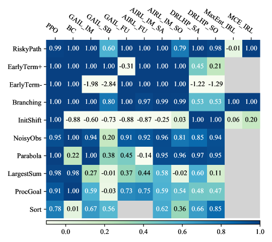
Figure 10: Mean episode return (across 15 seeds) of policy learned by each algorithm ($x$-axis) on each task ($y$-axis). Returns are normalized between $0.0$ for a random policy and $1.0$ for an optimal policy. Grey cells denote the algorithm being unable to run on that task (e.g. MaxEnt_IRL and MCE_IRL only run on small tabular tasks). See appendix C for full results and confidence intervals.

4.1 Experimental Setup

We evaluate a range of commonly used LfH algorithms: Maximum Entropy IRL (MaxEnt_IRL; Ziebart et al., 2008), Maximum Causal Entropy IRL (MCE_IRL; Ziebart, 2010), Behavioral Cloning (BC), Generative Adversarial Imitation Learning (GAIL; Ho and Ermon, 2016), Adversarial IRL (AIRL; Fu et al., 2018) and Deep Reinforcement Learning from Human Preferences (DRLHP; Christiano et al., 2017). We also present an RL baseline using Proximal Policy Optimization (PPO; Schulman et al., 2017).

We test several variants of these algorithms. We compare multiple implementations of AIRL (AIRL_IM and AIRL_FU) and GAIL (GAIL_IM, GAIL_FU and GAIL_SB). We also vary whether the reward function in AIRL_IM and DRLHP is state-only (AIRL_IM_SO and DRLHP_SO) or state-action (AIRL_IM_SA and DRLHP_SA). All other algorithms use state-action rewards.

We train DRLHP using preference comparisons from the ground-truth reward, and train all other algorithms using demonstrations from an optimal expert policy. We compute the expert policy using value iteration in discrete environments, and procedurally specify the expert in other environments. See appendix B for a complete description of the experimental setup and implementations.

4.2 Experimental Results

For brevity, we highlight a few notable findings, summarizing our results in Figure 10. See appendix C for the full results and a more comprehensive analysis.

Implementation Matters. Our results show that GAIL_IM and GAIL_SB are biased towards prolonging episodes: they achieve worse than random return on EarlyTerm-, where the optimal action is to end the episode, but match expert performance in EarlyTerm+. By contrast, GAIL_FU is biased towards ending the episode, succeeding in EarlyTerm- but failing in EarlyTerm+. This termination bias can be a major confounder when evaluating on variable-horizon tasks.

We also observe several other differences between implementations of the same algorithm. GAIL_SB achieves significantly lower return than GAIL_IM and GAIL_FU on NoisyObs, Parabola, LargestSum and ProcGoal. Moreover, AIRL_IM attains near-expert return on Parabola while AIRL_FU performs worse than random. These results confirm that implementation matters (Islam et al., 2017; Henderson et al., 2018; Engstrom et al., 2020), and illustrate how diagnostic tasks can pinpoint how performance varies between implementations.

Rewards vs Policy Learning. Behavioral cloning (BC), fitting a policy to demonstrations using supervised learning, exhibits bimodal performance. BC often attains near-optimal returns. However, in tasks with large continuous state spaces such as Parabola and Sort, BC performs close to random. We conjecture this is because BC has more difficulty generalizing to novel states than reward learning algorithms, which have an inductive bias towards goal-directed behavior.

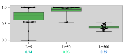
Figure 11: DRLHP_SA return on NoisyObs for varying numbers of noise dimensions $L$ (grid size $M=7$). We evaluate across 24 seeds trained for 3M timesteps. Mean returns are depicted as horizontal lines inside the boxes and reported underneath $x$-axis labels. Boxes span the 95% confidence intervals of the means; whiskers span the range of returns.

Exploration in Preference Comparison. We find DRLHP, which learns from preference comparisons, achieves lower returns in Branching than algorithms that learn from demonstrations. This is likely because Branching is a hard-exploration task: a specific sequence of actions must be taken in order to achieve a reward. For DRLHP to succeed, it must first discover this sequence, whereas algorithms that learn from demonstrations can simply mimic the expert.

While this problem is particularly acute in Branching, exploration is likely to limit the performance of DRLHP in other environments. To investigate this further, we varied the number of noise dimensions $L$ in NoisyObs from $5$ to $500$, reporting the performance of DRLHP_SA in Figure 11. Increasing $L$ decreases both the maximum and the variance of the return. This causes a higher mean return in $L=50$ than in $L=5$ (high variance) or $L=500$ (low maximum).

We conjecture this behavior is partly due to DRLHP comparing trajectories sampled from a policy optimized for its current best-guess reward. If the policy becomes low-entropy too soon, then DRLHP will fail to sufficiently explore. Adding stochasticity stabilizes the training process, but makes it harder to recover the true reward.

5 Case Study: Improving Implementations

In the previous section, we showed how DERAIL can be used to compare existing implementations of reward and imitation learning algorithms. However, benchmarks are also often used during the development of new algorithms and implementations. We believe diagnostic task suites are particularly well-suited to rapid prototyping. The tasks are lightweight so tests can be conducted quickly. Yet they are sufficiently varied to catch a wide range of bugs, and give a glimpse of effects in more complex environments. To illustrate this workflow, we present a case study refining an implementation of Deep Reinforcement Learning from Human Preferences (Christiano et al., 2017, DRLHP).

As discussed in section 4.2, the implementation we experimented with, DRLHP, has high-variance across random seeds. We conjecture this problem occurs because the preference queries are insufficiently diverse. The queries are sampled from rollouts of a policy, and so their diversity depends on the stochasticity of the environment and policy. Indeed, we see in Figure 11 that DRLHP is more stable when environment stochasticity increases.

The fundamental issue is that DRLHP’s query distribution depends on the policy, which is being trained to maximize DRLHP’s predicted reward. This entanglement makes the procedure liable to get stuck in local minima. Suppose that, mid-way through training, the policy chances upon some previously unseen, high-reward state. The predicted reward at this unseen state will be random – and so likely worse than a previously seen, medium-reward state. The policy will thus be trained to avoid this high-reward state – starving DRLHP of the queries that would allow it to learn in this region.

In an attempt to address this issue, we experiment with a few simple modifications to DRLHP:

• DRLHP_SLOW. Reduce the learning rate for the policy. The policy is initially high-entropy; over time, it learns to only take actions with high predicted reward. By slowing down policy learning, we maintain a higher-entropy query distribution.

• DRLHP_GREEDY. When sampling trajectories for preference comparison, use an $\epsilon$-greedy version of the current policy (with $\epsilon=0.1$). This directly increases the entropy of the query distribution.

• DRLHP_BONUS. Add an exploration bonus using random network distillation (Burda et al., 2019). Distillation steps are performed only on trajectories submitted for preference comparison. This has the effect of giving a bonus to state-action pairs that are uncommon in preference queries (even if they occurred frequently during policy training).

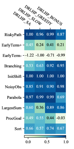
Figure 12: Return of DRLHP_SA and three variants: DRLHP_SLOW, slower policy training; DRLHP_GREEDY, $\epsilon$-greedy exploration; DRLHP_BONUS, exploration bonus (see section 5). Mean episode return (across 15 seeds) of policy learned by each algorithm ($x$-axis) on each task ($y$-axis). Returns are normalized between $0.0$ for a random policy and $1.0$ for an optimal policy.

We report the return achieved with these modifications in Figure 12. DRLHP_GREEDY produces the most stable results: the returns are all comparable to or substantially higher than the original DRLHP_SA. However, all modifications increase returns on hard-exploration task Branching, although for DRLHP_SLOW the improvement is modest. DRLHP_GREEDY and DRLHP_BONUS also enjoy significant improvements on high-dimensional classification task LargestSum, which likely benefits from more balanced labels. DRLHP_BONUS performs poorly on Parabola and ProcGoal: we conjecture that the large state space caused DRLHP_BONUS to explore excessively.

This case study shows how DERAIL can help rapidly test new prototypes, quickly confirming or discrediting a hypothesis of a how a change will affect a given algorithm. Moreover, we can gain a fine-grained understanding of performance along different axes. For example, we could conclude that DRLHP_BONUS does increase exploration (higher return on Branching) but may over-explore (lower return on ProcGoal). It would be difficult to disentangle these distinct effects in more complex environments.

6 Discussion

We have developed, to the best of our knowledge, the first suite of diagnostic environments for reward and imitation learning algorithms. We find that by isolating particular algorithmic capabilities, diagnostic tasks can provide a more nuanced picture of individual algorithms’ strengths and weaknesses than testing on more complex benchmarks. Our results confirm that reward and imitation learning algorithm performance is highly sensitive to implementation details. Furthermore, we have demonstrated the fragility of behavioral cloning, and obtained qualitative insights into the performance of preference-based reward learning. Finally, we have illustrated in a case study how DERAIL can support rapid prototyping of algorithmic refinements.

In designing the task suite, we have leveraged our personal experience as well as past work documenting design flaws and implementation bugs (Ziebart, 2010; Kostrikov et al., 2018). We expect to refine and extend the suite in response to user feedback, and we encourage other researchers to develop complementary tasks. Our environments are open-source and available at https://github.com/HumanCompatibleAI/seals.

Appendix A Full specification of tasks

A.1 RiskyPath

• State space: $\mathcal{S}{}=\{0,1,2,3\}$

• Action space: $\mathcal{A}{}=\{0,1\}$

• Horizon: $5$

• Dynamics:

  • $0\xrightarrow[]{0}1$, $0\xrightarrow[]{1}\begin{cases}1,&\text{50\% probability;}\\ 2,&\text{50\% probability.}\end{cases}$

  • $1\xrightarrow[]{0}2$, $1\xrightarrow[]{1}1$

  • $2\xrightarrow[]{a}2$ for all $a\in\mathcal{A}{}$

  • $3\xrightarrow[]{a}3$ for all $a\in\mathcal{A}{}$

• Rewards: $R(0)=R(1)=0,R(2)=1,R(3)=-100$

Figure A.1: RiskyPath

A.2 EarlyTerm$\pm$

• State space: $\mathcal{S}{}=\{0,1,2\}$

• Action space: $\mathcal{A}{}=\{0,1\}$

• Horizon: $10$

• Dynamics:

  • $0\xrightarrow[]{a}1$ for all $a\in\mathcal{A}{}$

  • $1\xrightarrow[]{0}0$, $1\xrightarrow[]{1}2$

• Rewards: $R(s)=1.0$ in EarlyTerm+
  and $R(s)=-1.0$ in EarlyTerm-

Figure A.2: EarlyTerm+

Figure A.3: EarlyTerm-

A.3 NoisyObs

• Configurable parameters: size $M=5$, noise length $L=20$

• State space: grid $\mathcal{S}{}=\mathbb{Z}_{M}\times\mathbb{Z}_{M}$, where $\mathbb{Z}_{M}=\{0,1,\cdots,M-1\}$

• Observations: $(x,y,z_{1},\cdots,z_{L})$, where:

  • $(x,y)\in\mathcal{S}{}$ are the state coordinates

  • $z_{i}$ are i.i.d. samples from the Gaussian $\mathcal{N}(0,1)$

• Action space: $\mathcal{A}{}=\{U,D,L,R,S\}$ for moving Up, Down, Left, Right or Stay (no-op).

• Horizon: $3M$

• Dynamics: Deterministic gridworld; attempting to move beyond boundary of world is a no-op.

• Rewards: $R(s)=\mathbbm{1}\left[s=\left(\lfloor\frac{M}{2}\rfloor,\lfloor\frac{M}{2}\rfloor\right)\right]$

• Initial state: $(0,0)$

Figure A.4: NoisyObs

A.4 Branching

• Configurable parameters: path length $L=10$, branching factor $B=2$

• State space: $\mathcal{S}{}=\{0,1,\cdots,LB\}$

• Action space: $\mathcal{A}{}=\{0,\cdots,B-1\}$

• Horizon: $L$

• Dynamics: $s\xrightarrow[]{a}s+(a+1)\cdot\mathbbm{1}[s\equiv 0\mod B]$

• Rewards: $R(s)=\mathbbm{1}\left[s=LB\right]$

• Initial state: $0$

Figure A.5: Branching

A.5 Parabola

• Configurable parameters: x-step $dx=0.05$, horizon $h=20$

• State space: $\mathcal{S}{}=\mathbbm{R}^{2}\times[-1,1]^{3}$

• Actions: $a\in(-\infty,+\infty)$

• Horizon: $h$

• Dynamics:

  $$\left((x,y),(c_{2},c_{1},c_{0})\right)\xrightarrow[]{a}\left((x+dx,y+a),(c_{2},c_{1},c_{0})\right)$$

• Rewards: $R(s)=(c_{2}x^{2}+c_{1}x+c_{0}-y)^{2}$

• Initial state: $(0,c_{0},c_{0},c_{1},c_{2})$, where $c_{i}\sim\operatorname{Unif}([-1,1])$

Figure A.6: Parabola

A.6 LargestSum

• Configurable parameters: half-length $L=25$

• State space: $\mathcal{S}{}=[0,1]^{2L}$

• Action space: $\mathcal{A}{}=\{0,1\}$

• Horizon: $1$

• Rewards: $R(s,a)=\mathbbm{1}\left[a=\mathbbm{1}\left[\sum_{j=1}^{L}s_{j}\leq\sum_{j=L+1}^{2L}s_{j}\right]\right]$

• Initial state: $s_{0}\sim\operatorname{Unif}\left([0,1]^{2L}\right)$

Figure A.7: LargestSum

A.7 InitShift

• State space: $\mathcal{S}{}=\{0,1,..,6\}$

• Action space: $\mathcal{A}{}=\{0,1\}$

• Horizon: $2$

• Dynamics: $s\xrightarrow[]{a}2s+1+a$

• Rewards:

  $$R(s)=\begin{dcases*}+1&if $s=3$\\ -1&if $s\in\{4,5\}$\\ +2&if $s=6$\\ 0&otherwise\end{dcases*}$$

• Initial state:
  

  • Expert: $0$

  • Learner: $1$

Figure A.8: InitShift

A.8 ProcGoal

• Configurable prameters: initial state bound $B=100$, goal distance $D=10$

• State space: $\mathcal{S}{}=\mathbb{Z}^{2}\times\mathbb{Z}^{2}$, where $(p,g)\in\mathcal{S}$ consists of agent position $p$ and goal position $g$

• Action space: $\mathcal{A}{}=\{U,D,L,R,S\}$ for moving Up, Down, Left, Right or Stay (no-op).

• Horizon: $3D$

• Dynamics: Deterministic gridworld on $p$; $g$ is fixed at start of episode.

• Rewards: $R((p,g))=-\lVert p-g\rVert_{1}$

• Initial state:

  • Position $p$ uniform over $\{p\in\mathbb{Z}^{2}:\lVert p\rVert_{1}\leq B\}$

  • Goal $g$ uniform over $\{g\in\mathbb{Z}^{2}:\lVert p-g\rVert_{1}=D\}$

Figure A.9: ProcGoal

A.9 Sort

• Configurable parameters: length $L=4$

• State space: $\mathcal{S}{}=[0,1]^{L}$

• Action space: $\mathcal{A}{}=\mathbb{Z}_{L}\times\mathbb{Z}_{L}$ where $\mathbb{Z}_{L}=\{0,..,L-1\}$

• Horizon: $2L$

• Dynamics: $a=(i,j)$ swaps elements $i$ and $j$

• Rewards: $R(s,s^{\prime})=\mathbbm{1}\left[c(s^{\prime})=n\right]+c(s^{\prime})-c(s)$, where $c(s)$ is the number of elements in the correct sorted position.

• Initial state: $s\sim\operatorname{Unif}([0,1]^{L})$

Figure A.10: Sort

Appendix B Experimental setup

B.1 Algorithms

The exact code for running the experiments and generating the plots can be found at https://github.com/HumanCompatibleAI/derail.

Imitation learning and IRL algorithms are trained using rollouts from an optimal policy. The number of expert timesteps provided is the same as the number of timesteps each algorithm runs for. For DRLHP, trajectories are compared using the ground-truth reward. The trajectory queries are generated from the policy being learned jointly with the reward.

We used open source implementations of these algorithms, as listed in Table B.1. We did not perform hyperparameter tuning, and relied on default values for most hyperparameters.

Source Code	Algorithms
Hill et al. [2018]	PPO, BC, GAIL_SB
Fu [2018]	AIRL_FU, GAIL_FU
Wang et al. [2020]	AIRL_IM_SA, AIRL_IM_SO, GAIL_IM, MCE_IRL, MaxEnt_IRL
Gleave [2020]	DRLHP_SA, DRLHP_SO

Table B.1: Sources of algorithm implementations (some of which were slightly adapted).

B.2 Evaluation

We run each algorithm with 15 different seeds and 500,000 timesteps. To evaluate a policy, we compute the exact expected episode return in discrete state environments. In other environments, we compute the average return over 1000 episodes. The score in a task is the mean return of the learned policy, normalized such that a policy taking random actions gets a score of 0.0 and the expert gets a score of 1.0. For EarlyTerm-, poor policies can reach values smaller than -3.0; to keep scores in a similar range to other tasks, we truncate negative values at -1.0.

Appendix C Complete experimental results

We provide results and analysis grouped around individually tasks (section C.1) and algorithms (section C.2). The results are presented using boxplot graphs, such as Figure C.1. The y-axis represents the return of the learned policy, while the $x$-axis contains different algorithms or tasks. Each point corresponds to a different seed. The means across seeds are represented as horizontal lines inside the boxes, with the boxes spanning bootstrapped $95\%$ confidence intervals of the means; the whiskers show the full range of returns. Each box is assigned a different color to aid in visually distinguishing the tasks; they do not have any semantic meaning.

C.1 Tasks

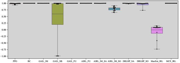
Figure C.1: RiskyPath: MaxEnt_IRL performs poorly as expected, while MCE_IRL performs well. Other algorithms evaluated look at state-action pairs individually, instead of looking at trajectories, avoiding the problem of risky behavior.

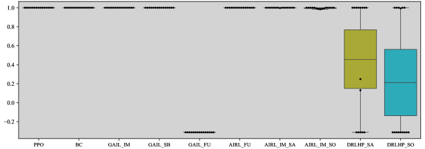
(a) EarlyTerm+

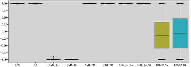
(b) EarlyTerm-

Figure C.2: EarlyTerm$\pm$: GAIL_FU performs worse than random in EarlyTerm+ and at expert level at EarlyTerm-, and we see the opposite behavior with GAIL_IM and GAIL_SB. This indicates that GAIL_FU has a negatively biased reward that favors episode termination, while GAIL_IM and GAIL_SB have a positively biased reward that favors survival. DRLHP also has extremely high variance, achieving both expert and random performance across different runs. This is because the implementation tested looks at segments of trajectories of the same length, without accounting for the fact that some segments will cause early termination. Instead, every segment is assigned the same reward, and the agent keeps their randomly initialized reward throughout the training process (which might by chance induce expert performance in such a simple environment).

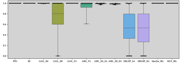
Figure C.3: Branching: algorithms that learn from expert demonstrations tend to perform well, since they require limited exploration. On the other hand, DRLHP can struggle to perform enough exploration to consistently find the goal and learn the correct reward. Note that DRLHP needs to find the goal multiple times in order to update the reward significantly.

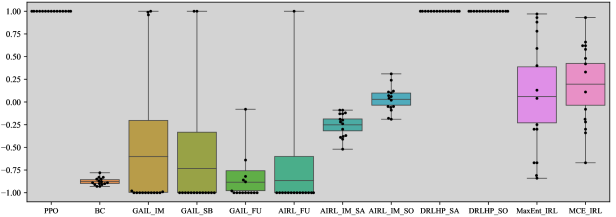
Figure C.4: InitShift: unlike Branching, in InitShift algorithms based on expert demonstrations fail, since the expert trajectories do not include the new initial state. By contrast, the task is trivial for DRLHP, which can compare trajectories generated at train time. Moreover, algorithms that learn state-action rewards from demonstrations perform worse than random. This is because the expert trajectories only contain action 1, and thus rewards tend to assign a positive weight to action $1$. However, the optimal action under the learners initial state distribution is to take action $0$. AIRL_IM_SO, MaxEnt_IRL and MCE_IRL learn state-only reward functions, and perform closer to the random policy.

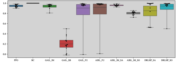
Figure C.5: NoisyObs: we see that BC achieves near-optimal performance, demonstrating that supervised learning can be more robust and sample-efficient in the presence of noise than other LfH algorithms. We also see that GAIL_SB performs poorly relative to GAIL_IM and GAIL_FU, which underscores the importance of the subtle differences between these implementations.

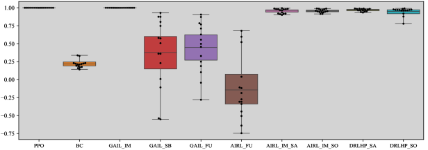
Figure C.6: Parabola: most algorithms perform well, except for BC, GAIL_SB and AIRL_FU.

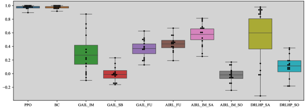
Figure C.7: LargestSum: Most algorithms fail to achieve expert performance, while BC does match expert performance, suggesting scaling algorithms like GAIL and AIRL to high-dimensional tasks may be a fruitful direction for future work. Methods using state-only reward functions, AIRL_SO and DRLHP_SO, perform poorly since the reward for this task depends on the actions taken.

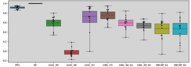
Figure C.8: ProcGoal: BC achieves expert performance, while most other algorithms get a reasonable, but lower score, while also exhibiting high variance between seeds. While this task requires generalization, the fact that the states and actions are discrete might make it easier for BC to generalize, compared to Parabola or Sort, where it performs poorly. One interesting result is AIRL_FU performing better than AIRL_IM_SA, while AIRL_IM_SA performs better than AIRL_FU in other tasks.

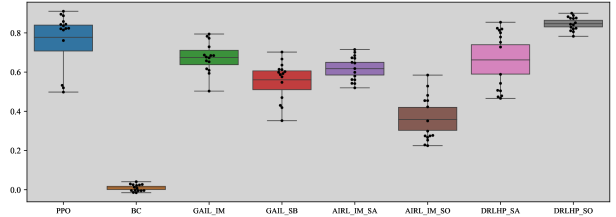
Figure C.9: Sort: Most algorithms achieve reasonable (but sub-expert) performance. Intriguingly DRLHP_SO achieves higher returns than most algorithms, with low-variance. Learning a good policy in this task is challenging, given that even PPO did not get at expert performance in all seeds. BC fails to get any reward. We also have that DRLHP_SO performs better than DRLHP_SA, while AIRL_IM_SA performs better than AIRL_IM_SO. Having a state-only reward might be easier to learn because there are less parameters and the groundtruth reward is indeed state-only, but state-action rewards can also incentivize the right policy by giving higher rewards to the correct action, making planning easier.

C.2 Algorithms

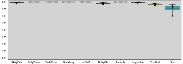
Figure C.10: PPO: serves as an RL baseline. We would expect most reward and imitation learning algorithms to obtain lower return, since they must learn a policy without knowing the reward. Most seeds achieve close to expert performance.

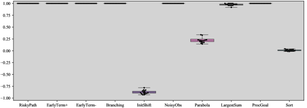
Figure C.11: BC: exhibits bimodal performance, either attaining near-expert return ($1.0$, normalized) in an environment or close to random ($0.0$). The return is similar across seeds. Behavioral cloning attains relatively low returns in Parabola and Sort, which have continuous observation spaces that require generalization and sequential decision making.

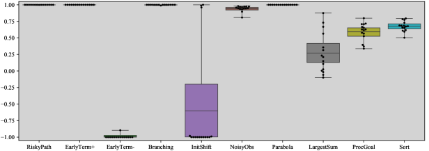
(a) GAIL_IM

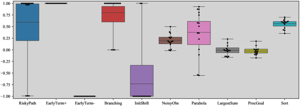
(b) GAIL_SB

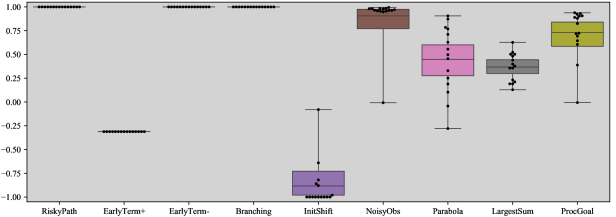
(c) GAIL_FU

Figure C.12: GAIL: GAIL_IM and GAIL_SB is positively biased, while GAIL_FU is negatively biased, in the sense discussed in Kostrikov et al. [2018]. We also see that GAIL_IM results dominate GAIL_SB, with GAIL_IM performing better on every task. There are no Sort results for GAIL_FU because this implementation did not support the pair action space used in Sort.

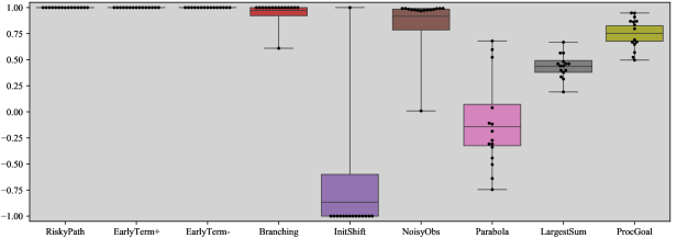
(a) AIRL_FU

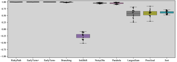
(b) AIRL_IM_SA

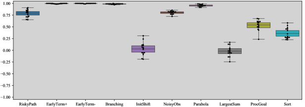
(c) AIRL_IM_SO

Figure C.13: AIRL: AIRL_IM_SA achieves higher returns than AIRL_IM_SO and AIRL_FU on the majority of environments. AIRL_FU obtains particularly low returns on Parabola. AIRL_IM_SA performs particularly well overall, with lower variance episode return than most algorithms while attaining high return in most tasks.

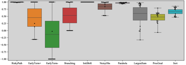
(a) DRLHP_SA

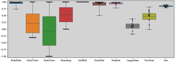
(b) DRLHP_SO

Figure C.14: DRLHP: achieves reasonable mean return, but exhibits high variance between seeds: some achieve expert performance while others are little better than random. Notably, DRLHP_SO is the highest scoring LfH algorithm we have tested in Sort. DRLHP performs poorly in Branching because of the difficulty of exploration, and in EarlyTerm$\pm$ because the implementation does not account for episode termination. It is the only algorithm we tested that succeeds in InitShift, as expected.

(a) DRLHP_SLOW

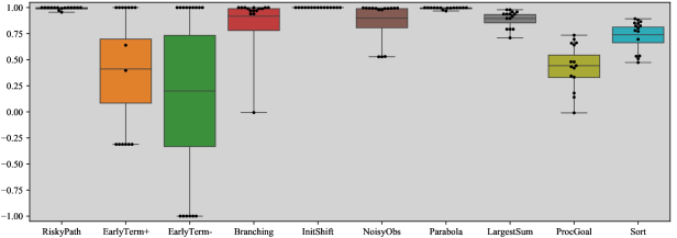
(b) DRLHP_GREEDY

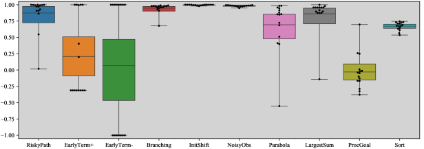
(c) DRLHP_BONUS

Figure C.15: DRLHP modifications: all versions improve the scores on NoisyObs; DRLHP_GREEDY and DRLHP_BONUS get better scores on Branching and LargestSum. DRLHP_GREEDY achives greater or similar scores to DRLHP_SA in all tasks. Further discussion of these results can be found in Section 5.

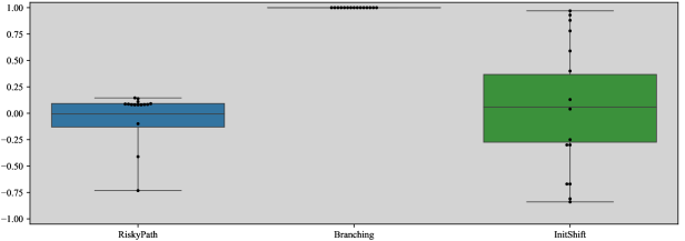
Figure C.16: Tabular IRL: executed only on tasks with discrete state and action spaces and fixed horizon. As expected, MaxEnt_IRL obtains a low return in RiskyPath. For InitShift, the expert demonstrations do not provide information to choose between the subset of states accessible during learning, and so the algorithm gets a random score that depends on the randomly initialized initial reward.

References

- Burda et al. [2019] Yuri Burda, Harrison Edwards, Amos Storkey, and Oleg Klimov. Exploration by random network distillation. In International Conference on Learning Representations, 2019. URL https://openreview.net/forum?id=H1lJJnR5Ym.
- Cabi et al. [2019] Serkan Cabi, Sergio Gómez Colmenarejo, Alexander Novikov, Ksenia Konyushkova, Scott Reed, Rae Jeong, Konrad Zolna, Yusuf Aytar, David Budden, Mel Vecerik, Oleg Sushkov, David Barker, Jonathan Scholz, Misha Denil, Nando de Freitas, and Ziyu Wang. A framework for data-driven robotics. arXiv: 1909.12200v1 [cs.RO], 2019.
- Christiano et al. [2017] Paul F Christiano, Jan Leike, Tom Brown, Miljan Martic, Shane Legg, and Dario Amodei. Deep reinforcement learning from human preferences. In NIPS, pages 4299–4307, 2017.
- Engstrom et al. [2020] Logan Engstrom, Andrew Ilyas, Shibani Santurkar, Dimitris Tsipras, Firdaus Janoos, Larry Rudolph, and Aleksander Madry. Implementation matters in deep RL: A case study on PPO and TRPO. In ICLR, 2020. URL https://openreview.net/forum?id=r1etN1rtPB.
- Fu [2018] Justin Fu. Inverse RL: Implementations for imitation learning/IRL algorithms in rllab. https://github.com/justinjfu/inverse_rl, 2018.
- Fu et al. [2018] Justin Fu, Katie Luo, and Sergey Levine. Learning robust rewards with adverserial inverse reinforcement learning. In ICLR, 2018.
- Gleave [2020] Adam Gleave. Evaluating rewards: comparing and evaluating reward models. https://github.com/humancompatibleai/evaluating-rewards, 2020.
- Guyon and Elisseeff [2003] Isabelle Guyon and André Elisseeff. An introduction to variable and feature selection. JMLR, pages 1157–1182, 3 2003.
- Henderson et al. [2018] Peter Henderson, Riashat Islam, Philip Bachman, Joelle Pineau, Doina Precup, and David Meger. Deep reinforcement learning that matters. In AAAI, 2018.
- Hill et al. [2018] Ashley Hill, Antonin Raffin, Maximilian Ernestus, Adam Gleave, Anssi Kanervisto, Rene Traore, Prafulla Dhariwal, Christopher Hesse, Oleg Klimov, Alex Nichol, Matthias Plappert, Alec Radford, John Schulman, Szymon Sidor, and Yuhuai Wu. Stable Baselines. https://github.com/hill-a/stable-baselines, 2018.
- Ho and Ermon [2016] Jonathan Ho and Stefano Ermon. Generative adversarial imitation learning. In NIPS, pages 4565–4573, 2016.
- Islam et al. [2017] Riashat Islam, Peter Henderson, Maziar Gomrokchi, and Doina Precup. Reproducibility of benchmarked deep reinforcement learning tasks for continuous control. arXiv preprint arXiv:1708.04133, 2017.
- James et al. [2020] Stephen James, Zicong Ma, David Rovick Arrojo, and Andrew J. Davison. Rlbench: The robot learning benchmark learning environment. IEEE Robotics and Automation Letters, 5(2):3019–3026, 2020.
- Johnson et al. [2017] Justin Johnson, Bharath Hariharan, Laurens van der Maaten, Li Fei-Fei, C. Lawrence Zitnick, and Ross Girshick. CLEVR: A diagnostic dataset for compositional language and elementary visual reasoning. In CVPR, 2017.
- Kostrikov et al. [2018] Ilya Kostrikov, Kumar Krishna Agrawal, Debidatta Dwibedi, Sergey Levine, and Jonathan Tompson. Discriminator-actor-critic: Addressing sample inefficiency and reward bias in adversarial imitation learning. arXiv preprint arXiv:1809.02925, 2018.
- Kottur et al. [2019] Satwik Kottur, José M. F. Moura, Devi Parikh, Dhruv Batra, and Marcus Rohrbach. CLEVR-Dialog: A diagnostic dataset for multi-round reasoning in visual dialog. In NAACL-HLT, 2019.
- Liu et al. [2019] Runtao Liu, Chenxi Liu, Yutong Bai, and Alan L. Yuille. CLEVR-Ref+: Diagnosing visual reasoning with referring expressions. In CVPR, 2019.
- Memmesheimer et al. [2019] Raphael Memmesheimer, Ivanna Kramer, Viktor Seib, and Dietrich Paulus. Simitate: A hybrid imitation learning benchmark. In IROS, pages 5243–5249, 2019.
- Myers et al. [2011] Glenford J Myers, Corey Sandler, and Tom Badgett. The art of software testing, chapter 5. John Wiley & Sons, 2011.
- Ng and Russell [2000] Andrew Y. Ng and Stuart Russell. Algorithms for inverse reinforcement learning. In ICML, 2000.
- OpenAI et al. [2019] OpenAI, Ilge Akkaya, Marcin Andrychowicz, Maciek Chociej, Mateusz Litwin, Bob McGrew, Arthur Petron, Alex Paino, Matthias Plappert, Glenn Powell, Raphael Ribas, Jonas Schneider, Nikolas Tezak, Jerry Tworek, Peter Welinder, Lilian Weng, Qiming Yuan, Wojciech Zaremba, and Lei Zhang. Solving Rubik’s Cube with a robot hand. arXiv: 1910.07113v1 [cs.LG], 2019.
- Osband et al. [2020] Ian Osband, Yotam Doron, Matteo Hessel, John Aslanides, Eren Sezener, Andre Saraiva, Katrina McKinney, Tor Lattimore, Csaba Szepesvari, Satinder Singh, Benjamin Van Roy, Richard Sutton, David Silver, and Hado Van Hasselt. Behaviour suite for reinforcement learning. In ICLR, 2020.
- Reddy et al. [2020] Siddharth Reddy, Anca D. Dragan, and Sergey Levine. SQIL: Imitation learning via reinforcement learning with sparse rewards. In ICLR, 2020.
- Ross et al. [2011] Stephane Ross, Geoffrey Gordon, and Drew Bagnell. A reduction of imitation learning and structured prediction to no-regret online learning. In AISTATS, 2011.
- Schulman et al. [2017] John Schulman, Filip Wolski, Prafulla Dhariwal, Alec Radford, and Oleg Klimov. Proximal policy optimization algorithms. arXiv:1707.06347v2 [cs.LG], 2017.
- Silver et al. [2016] David Silver, Aja Huang, Chris J. Maddison, Arthur Guez, Laurent Sifre, George van den Driessche, Julian Schrittwieser, Ioannis Antonoglou, Veda Panneershelvam, Marc Lanctot, Sander Dieleman, Dominik Grewe, John Nham, Nal Kalchbrenner, Ilya Sutskever, Timothy Lillicrap, Madeleine Leach, Koray Kavukcuoglu, Thore Graepel, and Demis Hassabis. Mastering the game of Go with deep neural networks and tree search. Nature, 529(7587):484–489, 2016.
- Sinha et al. [2019] Koustuv Sinha, Shagun Sodhani, Jin Dong, Joelle Pineau, and William L. Hamilton. CLUTRR: A diagnostic benchmark for inductive reasoning from text. In EMNLP, 2019.
- Vinyals et al. [2019] Oriol Vinyals, Igor Babuschkin, Wojciech M. Czarnecki, Michaël Mathieu, Andrew Dudzik, Junyoung Chung, David H. Choi, Richard Powell, Timo Ewalds, Petko Georgiev, Junhyuk Oh, Dan Horgan, Manuel Kroiss, Ivo Danihelka, Aja Huang, Laurent Sifre, Trevor Cai, John P. Agapiou, Max Jaderberg, Alexander S. Vezhnevets, Rémi Leblond, Tobias Pohlen, Valentin Dalibard, David Budden, Yury Sulsky, James Molloy, Tom L. Paine, Caglar Gulcehre, Ziyu Wang, Tobias Pfaff, Yuhuai Wu, Roman Ring, Dani Yogatama, Dario Wünsch, Katrina McKinney, Oliver Smith, Tom Schaul, Timothy Lillicrap, Koray Kavukcuoglu, Demis Hassabis, Chris Apps, and David Silver. Grandmaster level in StarCraft II using multi-agent reinforcement learning. Nature, 575(7782):350–354, 2019.
- Wacker [2015] Mike Wacker. Just say no to more end-to-end tests. Google Testing Blog, 2015. URL https://testing.googleblog.com/2015/04/just-say-no-to-more-end-to-end-tests.html.
- Wang et al. [2019] Alex Wang, Amanpreet Singh, Julian Michael, Felix Hill, Omer Levy, and Samuel R. Bowman. GLUE: A multi-task benchmark and analysis platform for natural language understanding. In ICLR, 2019.
- Wang et al. [2020] Steven Wang, Adam Gleave, and Sam Toyer. imitation: implementations of inverse reinforcement learning and imitation learning algorithms. https://github.com/humancompatibleai/imitation, 2020.
- Ziebart [2010] Brian D Ziebart. Modeling purposeful adaptive behavior with the principle of maximum causal entropy. PhD thesis, Carnegie Mellon University, 2010.
- Ziebart et al. [2008] Brian D. Ziebart, Andrew Maas, J. Andrew Bagnell, and Anind K. Dey. Maximum entropy inverse reinforcement learning. In AAAI, 2008.