When Will an Elevator Arrive?

Abstract

We present and analyze a minimalist model for the vertical transport of people in a tall building by elevators. We focus on start-of-day operation in which people arrive at the ground floor of the building at a fixed rate. When an elevator arrives on the ground floor, passengers enter until the elevator capacity is reached, and then they are transported to their destination floors. We determine the distribution of times that each person waits until an elevator arrives, the number of people waiting for elevators, and transition to synchrony for multiple elevators when the arrival rate of people is sufficiently large. We validate many of our predictions by event-driven simulations.

1 Introduction

How long until the next elevator arrives? Many of us ponder this question as we wait in the lobby of a tall building before getting to our destination floor. The impact of waiting for elevators is increasing because of the continued expansion of cities and high-rise buildings. In Tokyo, New York, and Hong Kong, for example, there are currently about 190,000 [1], 84,000 [2], and 69,000 [3] elevators, respectively. In the extraordinarily vertical city of Hong Kong, their number is increasing at a rate of about 1500 per year [3]. Thus the carrying capabilities of building elevators necessarily represents an important feature of building design.

Despite the considerable development of electric elevators since their inception in the 1880s, as well as their increasing importance in contemporary society, our understanding of the transport properties of elevators is incomplete. There has been much work from the engineering and operations research perspectives on elevators, including their control and scheduling in tall buildings (see, e.g., [4, 5, 6, 7, 8, 9, 10, 11, 12]). Studies of this genre typically focus either on simulations of realistic scenarios or on the control mechanisms for multi-elevator systems. However, such investigations do not provide insights on the performance of such systems as a function of basic parameters, such as the passenger demand, as well as elevator and building characteristics. The physics-based literature on the dynamics of elevators has been either primarily numerical in character [13] or invokes analogies to dynamical systems theory [14, 15].

In this work, we present a simple-minded probabilistic approach to treat a demand-driven elevator system and develop insights about the performance of such a system. We focus on the start of a workday, in which people enter a building lobby at a given rate and want to get to their destination floors. This scenario is sufficiently simple that some analytical results can be obtained, yet this case still reflects realistic aspects of elevator operation. Within a minimal model to be defined in the next section, we determine the distribution of times that one has to wait for an elevator and its dependence on the arrival rate of individuals, the number of elevators, and the capacity of each elevator. We validate many of our predictions by event-driven simulations. We also examine the conditions under which multiple elevators tend to synchronize. This latter property bears some resemblance to the clustering phenomenon that occurs in subways and along bus routes [16], where many full vehicles arrive in quick succession at a subway station or a bus stop, followed by a long period with no vehicles arriving.

In the next section, we outline our model. In Sec. 3, we treat the dynamics in the simplifying case of a single infinite-capacity elevator. We derive the time of a single elevator cycle and its distribution, as well as the distribution of the number of passengers in the elevator. We then turn to the case of a single finite-capacity elevator in Sec. 4, where we first discuss the condition for a steady state, and then present basic dynamical properties, such as the “clearing” time—the time interval between events where all waiting passengers are accommodated in the elevator that is currently loading—and the clearing probability, as well as the occupancy distributions in the lobby and in the elevator. In Sec. 5, we treat the realistic situation of many finite-capacity elevators. We determine the steady-state condition and then investigate how synchronization can occur. Some concluding remarks are given in Sec. 6

2 Model

Our model is based on the following assumptions (Fig. 1):

1. Start-of-day operation: the building is initially unoccupied, and individuals arrive at the ground floor lobby according to a Poisson process at rate $\lambda$.

2. When an elevator reaches the lobby, it is filled on a first-come/first-serve basis until either all passengers are accommodated or the elevator reaches its capacity $C$.

3. The building has $F$ floors and $k$ identical elevators that can access all floors.

4. Each person has a distinct destination floor that is uniformly distributed in $[1,F]$.

5. The time for an elevator to travel one floor is $\tau_{e}$.

6. Each elevator stop requires a time $\tau_{s}$ per entering and exiting person that is independent of the elevator occupancy.

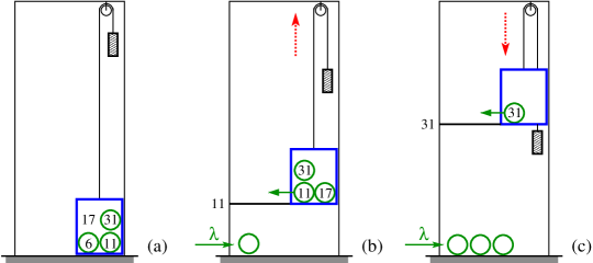
Figure 1: Cartoon of single-elevator transport during start-of-day operation where passengers arrive at rate $\lambda$: (a) Passengers (circles) just after entering the elevator; the numbers indicate destination floors. (b) A passenger leaves the elevator at her/his destination ($11^{\rm th}$) floor. (c) After the last passenger leaves, the elevator returns to the ground floor.

While most of these features of the model accord with everyday experience, various approximations have been made and other relevant attributes have been neglected. These include: (a) In some tall buildings, some elevators only stop at a subset of all floors. This restriction vaguely resembles staging in a multistage rocket [17, 18], a device that leads to greater efficiency. (b) The time to enter and exit an elevator is not constant, but is clearly an increasing function of its occupancy. (c) Most skyscrapers have a smaller floor area in the higher stories, so the distribution of destination floors is not uniform. (d) Travel between different building floors or from an upper floor back to the lobby is not treated. Incorporating all these features would be more realistic, but such a generalization would greatly complicate theoretical modeling. For both parsimony and tractability, we only include the elements (i)–(vi) listed above. Another desirable feature of this minimalist model is that it can be simulated with great efficiency by an event-driven approach (see A for details).

3 Single Infinite-Capacity Elevator

We first investigate the idealized case of a building with a single unlimited-capacity elevator. While patently unrealistic, this situation provides the starting point for treating finite-capacity elevators and multi-elevator buildings. With a single infinite-capacity elevator, a steady state is eventually achieved in which the average time for the elevator to complete a single cycle, i.e., return to the ground floor, equals the average number of people who arrive in the lobby during a cycle. Note that the infinite-capacity case is equivalent to the individual arrival rate $\lambda$ being sufficiently small that a finite elevator capacity is never reached. We now determine basic features of this steady state.

3.1 The cycle time

A single cycle of an elevator involves the following steps (Figs. 1 & 2):

1. The elevator arrives on the ground (lobby) floor.

2. Waiting passengers in the lobby enter the elevator.

3. The elevator delivers each passenger to her/his destination floor in ascending order and passengers with this destination floor exit.

4. When the elevator empties, it returns to the ground floor and a cycle begins anew.

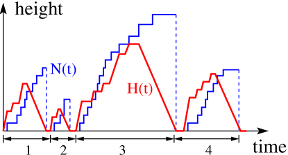
Figure 2: Schematic time dependence of the number of passengers, $N(T)$, in the lobby (blue) and the elevator height, $H(t)$ (red). Four elevator cycles are indicated.

We first determine the time for a single elevator cycle when $N$ passengers have entered the elevator. This cycle time is obviously an increasing function of $N$, and two factors contribute to this $N$ dependence. First, the total time that the elevator is stopped to pick up and discharge passengers in a single cycle in $2N\tau_{s}$. Second, for increasing $N$, it is more likely that the elevator goes to a higher floor to discharge the last passenger with the highest destination floor. For $N\gg 1$ passengers, we use extreme-value statistics [19, 20] to find that the expected highest destination floor among $N\gg 1$ passengers is given by

$$F_{\rm max}=F\,\frac{N}{N+1}\,.$$

Consequently, the expected time for the elevator to complete a single cycle is

$$T(N) =2F_{\rm max}\,\tau_{e}+2N\tau_{s}=2F\tau_{e}\,\frac{N}{N+1}+2N\tau_{s}\,.$$ (1)

To obtain a rough estimate of the cycle time, we use that $\tau_{e}=1\,$sec, $\tau_{s}=2.5\,$sec, and $F=100$ floors; these are representative numbers for elevators in a tall building [21]. The cycle time is then $T(N)=200N/(N\!+\!1)+5N$. For $N=20$ passengers, which is typical for a high-capacity elevator, the expected time for one elevator cycle is $T(20)\approx 290\,$sec $\approx 5\,$min. Henceforth, we fix $\tau_{e}=1$ for simplicity, so that $\tau_{s}$ becomes the ratio of the single-passenger entrance/exit time to the single-floor travel time.

3.2 The steady state

In a single cycle of duration $T$, $\lambda T$ new passengers typically arrive after the elevator leaves before is returns. The steady-state occupancy of an elevator, $N_{\rm ss}$, is determined by equating $\lambda T(N)$ in Eq. (1) with $N$. This gives

$$\lambda\left[2F\Big{(}\frac{N_{\rm ss}}{N_{\rm ss}+1}\Big{)}+2N_{\rm ss}\tau_{s}\right]=N_{\rm ss}\,,$$

from which

$$N_{\rm ss}=\frac{2\lambda F}{1-2\lambda\tau_{s}}-1\,.$$ (2)

A basic consequence of this simple calculation is the existence of a critical arrival rate $\lambda_{c}=1/2\tau_{s}$. When the arrival rate exceeds $\lambda_{c}$, progressively more passengers will be waiting for the elevator after each successive cycle and no steady state is possible.

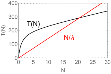
Figure 3: Dependence of the elevator cycle time $T(N)$ in Eq. (1) on $N$ for $\tau_{e}=1\,$sec, $\tau_{s}=2.5\,$sec and $F=100$ floors. A steady state arises when $T(N)$ intersects the line $N/\lambda$, which occurs for $\lambda<\lambda_{c}=1/5$ for these parameters. In this example $\lambda=0.07<\lambda_{c}$

It may be surprising at first sight that the critical arrival rate does not depend on the building height. This independence occurs because of the infinite elevator capacity and because the travel time, $2NF/(N\!+\!1)$, becomes a constant contribution to the total cycle time for large $N$, which becomes negligible for $N\to\infty$. Consequently, the dependence on building height disappears. As a numerical example, for $F=100$ and $\tau_{s}=2.5$, $N_{\rm ss}=200\lambda/(1-5\lambda)-1$. For a steady-state elevator occupancy of $N_{\rm ss}=20$, $\lambda=21/305\approx 0.07$ (the intersection point in Fig. 3). Thus this single-elevator system is not close to its transport limit of $\lambda_{c}=1/5$ when $N_{\rm ss}=20$. Since all waiting passengers can fit on the elevator, the longest that any passenger has to wait is one complete cycle; this occurs when the next passenger arrives just after the elevator has departed.

3.3 Cycle and occupancy distributions

To compute the distribution of cycle times, we use Eq. (1) to write the maximum floor reached by the elevator in terms of $N$ and the cycle time: $F_{\rm max}=\frac{1}{2}(T-2N\tau_{s})$. When the distribution of destination floors is uniformly distributed in $[1,F]$, the probability that the maximum floor reached by an elevator with $N$ passengers is [19, 20]

$$M(F_{\rm max})=\frac{N}{F}\left[\frac{F_{\rm max}}{F}\right]^{N-1}\,.$$ (3)

Since we are considering tall buildings, the assumption $F\gg 1$ is implicit.

We now use $M(F_{\rm max})\,dF_{\rm max}=P(T)\,dT$, with $P(T)$ defined as the cycle-time distribution, to eliminate $F_{\rm max}$ in favor of $T$ to determine $P(T)$. To compute the distribution of times for the $i^{\rm th}$ cycle, $P_{i}(T)$, we must sum over the possible values of $N$ in a given cycle. This leads to

$$P_{i}(T)=\sum_{N=1}^{T/2\tau_{s}}\frac{N}{2F}\left[\frac{\frac{1}{2}(T-N\tau_{s})}{F}\right]^{N-1}Q_{i}(N)\,,$$ (4a)

where $$Q_{i}(N) N i^{\rm th}$$ is the probability that the elevator has passengers in the cycle. The upper limit on the sum corresponds to all occupants of the elevator having the smallest possible destination floor. Equivalently, this limit corresponds to the maximum number of passengers that can be accommodated for a given cycle time.

Because new passengers arrive at rate $\lambda$, the probability $Q_{i}(N)$ is given by the Poisson distribution that is integrated over all possible values of the previous cycle time:

$$Q_{i}(N)=\int dT\,e^{-\lambda T}\,\frac{(\lambda T)^{N}}{N!}\,P_{i-1}(T)\,.$$ (4b)

That is, the number of passengers waiting for the $i^{\rm th}$ cycle of the elevator depends on the $(i-1)^{\rm st}$ cycle time. In turn, the parameters in the $(i-1)^{\rm st}$ cycle depend on the parameters in the $(i-2)^{\rm nd}$ cycle. Thus the distributions $P_{i}(T)$ and $Q_{i}(N)$ have to be determined iteratively.

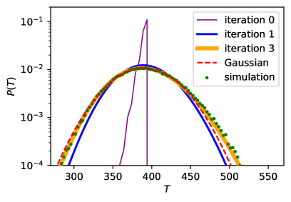
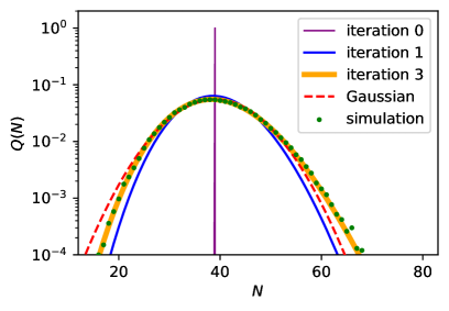
Figure 4: (a) The cycle time distribution $P(T)$ (binned to eliminate artificial spikes) and (b) the occupancy distribution $Q(N)$ for the case of arrival rate $\lambda=\lambda_{c}$/2, with $\tau_{s}=2.5$ for all passengers. For rapid convergence, the initial condition is chosen to be the steady-state occupancy, $N_{0}=N_{ss}=39$.

To illustrate this iterative approach, suppose that initially there are $N_{0}$ passengers waiting for the elevator. Then the probability distribution for the time of this zeroth cycle is

$$P_{0}(T)=\frac{N_{0}}{2F}\left[\frac{\frac{1}{2}(T-N_{0}\tau_{s})}{F}\right]^{N_{0}-1}\,.$$

Correspondingly, the probability that $N$ passengers waiting for the elevator at the start of the first cycle is

$$Q_{1}(N)=\int dT\,e^{-\lambda T}\,\frac{(\lambda T)^{N}}{N!}\,\frac{N_{0}}{F}\left[\frac{\frac{1}{2}(T-N_{0}\tau_{s})}{F}\right]^{N_{0}-1}\,.$$

Using Eqs. (4), we iterate to give the distributions of $N$ and $T$ in successive elevator cycles. Numerically, this iteration quickly converges to a steady state (Fig. 4). By making the assumption of a steady state, we may write closed equations for the distributions $P$ and $Q$ by dropping the subscript and eliminating $Q$ in the equation for $P$ (and vice versa). We thereby find the implicit solutions:

$$\begin{split}P(T)&=\int_{0}^{T/2\tau_{s}}dx\,\,\frac{x}{2F}\left[\frac{\frac{1}{2}(T-x\tau_{s})}{F}\right]^{x-1}\int_{0}^{\infty}dy\,\,\!e^{-\lambda y}\,\,\frac{(\lambda y)^{x}}{x!}\,P(y)\,,\\[5.69054pt] Q(N)&=\int_{0}^{\infty}dy\,e^{-\lambda y}\int_{0}^{T/2\tau_{s}}dx\,\,\frac{x}{2F}\left[\frac{\frac{1}{2}(T-x\tau_{s})}{F}\right]^{x-1}\!\frac{(\lambda y)^{x}}{x!}\,Q(x)\,.\end{split}$$ (5)

In our numerical solutions, we found it simpler, however, to iterate Eqs. (4) to find the steady-state distributions, the results of which are shown in Fig. 4.

In terms of the cycle time distribution, we can now determine the more relevant distribution of times that an individual has to wait before an elevator arrives. Since an individual arrives equiprobably during an elevator cycle, her/his waiting time is uniformly distributed in the range $[0,T]$ for a given elevator cycle time $T$. We now average this uniform distribution over all cycle times of duration $t$ or larger to obtain the individual waiting time distribution, which we define as $\mathcal{W}(t)$:

$$\mathcal{W}(t)=\int_{t}^{\infty}\frac{P(T)}{T}\,dT\,.$$ (6)

For the peaked and close-to-Gaussian cycle time distribution in Fig. 4(a), the waiting time distribution resembles the Fermi-Dirac distribution at low temperatures—nearly constant for small times and then rapidly cut off beyond the average cycle time.

3.4 Fluctuations

As shown in previous section, the cycle time and occupancy distributions quickly converge to steady-state forms with well-localized peaks. We can determine the widths of these two distributions by using the mean values $T_{ss}$ and $N_{ss}$ from Sec. 3.2, exploiting the Poissonian nature of the distribution for $N$, and also making use the law of total variance [22].

We denote $E(x)=\langle x\rangle$ as the mean value of the variable $x$ and ${\rm Var}(x)=\langle x^{2}\rangle-\langle x\rangle^{2}$ as its variance. Because the distribution of $N$ is Poissonian with mean value $\lambda T$ for a given value of the travel time $T$, ${\rm Var}(N|T)=\lambda T$. The law of total variance states that ${\rm Var}(N)={\rm E}\big{(}{\rm Var}(N|T)\big{)}+{\rm Var}\big{(}{\rm E}(N|T)\big{)}$ [22]. For the elevator system, this gives

$${\rm Var}(N) ={\rm E}\big{(}{\rm Var}(N|T)\big{)}+{\rm Var}\big{(}{\rm E}(N|T)\big{)}$$

$$=\lambda{\rm E}(T)+{\rm Var}(\lambda T)$$

$$=N_{ss}+\lambda^{2}{\rm Var}(T)\ .$$ (7)

Since the elevator cycle time equals $T=2F_{\rm max}+2N\tau_{s}$ for a given value of $N$, the law of total variance for $T$ now leads to

$${\rm Var}(T) ={\rm E}\big{(}{\rm Var}(T|N)\big{)}+{\rm Var}\big{(}{\rm E}(T|N)\big{)}$$

$$={\rm E}\big{(}{\rm Var}(2F_{\rm max})+2N\tau_{s}\big{)}+{\rm Var}(2F_{\rm max}+2N\tau_{s})$$

$$=4{\rm E}\big{(}{\rm Var}(F_{\rm max})\big{)}+4\tau_{s}^{2}\,{\rm Var}(N)\ .$$

We now use the distribution (3) for $F_{\rm max}$ to compute the $\text{Var}(F_{\rm max})$ and obtain

$${\rm Var}(F_{\rm max})={{NF^{2}}/\big{[}{(N+1)^{2}(N+2)}\big{]}}~{}\underset{N\to\infty}{\longrightarrow}~{}\left({F}/{N}\right)^{2}\,.$$

Thus

$${\rm Var}(T)=4\left({F}/{N_{ss}}\right)^{2}+4\tau_{s}^{2}\,{\rm Var}(N)\ .$$ (8)

Substituting (8) in (7) and also using (8) itself, we finally have

$$\begin{split}{\rm Var}(T)&=4\left(\frac{F}{N_{ss}}\right)^{2}+4\tau_{s}^{2}\big{[}\lambda T_{ss}+\lambda^{2}{\rm Var}(T)\big{]}=\frac{4(F/N_{ss})^{2}+4\tau_{s}^{2}N_{ss}}{1-4\tau_{s}^{2}\lambda^{2}}\ ,\\ {\rm Var}(N)&=N_{ss}+\frac{4\lambda^{2}(F/N_{ss})^{2}+4\lambda^{2}\tau_{s}^{2}N_{ss}}{1-4\tau_{s}^{2}\lambda^{2}}\ .\end{split}$$ (9)

We now numerically estimate Var$(T)$ and Var$(N)$ and compare with Fig. 4. In this figure, $\lambda=\lambda_{c}/2$, which leads to $N_{ss}=39$. The cycle time from (1) then is $T(39)=390$. Using $\tau_{s}=2.5$ and $F=100$, we obtain ${\rm Var}(T)\approx 1335$ and ${\rm Var}(N)\approx 53$. Consequently, the waiting time between successive arrivals of the elevator will typically be in the range 390 sec $\pm$ 36 sec, while the number of passengers in the elevator will be 39 $\pm$ 7. These numbers are in accord with the simulated distributions in Fig. 4. Thus fluctuations in the cycle time and occupancy are substantial, but do not dominate the steady-state behavior.

4 Single Finite-Capacity Elevator

We now turn to the slightly more realistic case of a single elevator with a finite capacity $C$. This discussion serves as a starting point to treat multiple identical elevators.

4.1 The steady state

For a single elevator in the steady state, the average number of passengers waiting when the elevator arrives at the ground floor must be less than or equal to $C$. At the stability limit, the elevator should be filled to capacity. Thus a steady state should arise whenever $\lambda T(C)\leq C$, where $T(C)$ is the cycle time for an elevator filled to capacity and $\lambda$ is again the passenger arrival rate. Using Eq. $\eqref{TN}$ for $T(C)$, we have

$$\lambda\leq\lambda_{c}=\frac{1}{2\tau_{s}+2F/(C+1)}\,.$$ (10)

For an elevator of capacity $C=20$ and using $\tau_{s}=2.5\,$sec, $F=100$, the steady-state criterion gives $\lambda\leq 0.0689$. Thus, for a single elevator, the critical arrival rate is reduced by nearly a factor of 3 compared to an infinite-capacity elevator, where $\lambda_{c}=1/5$ (Sec. 3.2). A critical rate of $\lambda_{c}\approx 0.07$ corresponds to an unrealistically small arrival rate of approximately 1 passenger every 15 seconds. Clearly, and as we all have experienced, many elevators are needed to service a tall office building, as will be discussed in Sec. 5

4.2 The clearing time

A basic characteristic of single-elevator dynamics is the “clearing” time, defined as the time interval between the successive events where the lobby is emptied when the elevator leaves the ground floor (Fig. 5). When the elevator takes on passengers, the number of waiting passengers $N(t)$ suddenly decreases by $C$, if the number of waiting passengers exceeds the elevator capacity, or by $N(t)$, otherwise. For the example shown in the figure, there is a transient buildup of waiting passengers who have to wait more than one cycle, under the first come/first serve assumption, before boarding an elevator. Eventually, the situation arises in the sixth cycle where $N(t)<C$, at which point the lobby is cleared when the elevator leaves.

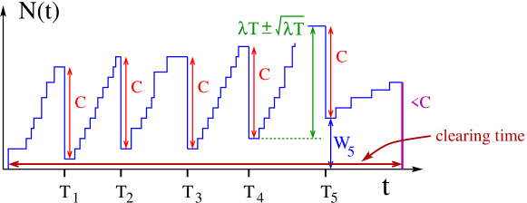
Figure 5: Schematic illustration of the time dependence of the number of people $N(t)$ waiting on the ground floor over six elevator cycles, with clearing occurring at the sixth cycle. The number of new passengers accumulated in each cycle is $\lambda T\pm\sqrt{\lambda T}$, while at most $C$ passengers are removed in each cycle.

To determine the clearing time, we appeal to an equivalence between the buildup and removal of passengers in the lobby and a random walk process. Consider first the case where the arrival rate equals its critical value, for which $\lambda_{c}T=C$. Thus the buildup of passengers in the lobby during one elevator cycle and the removal of waiting passengers when an elevator is loaded are, on average, equal. Let $W_{n}$ denote the number of people still waiting in the lobby after the $n^{\rm th}$ cycle. Note that whenever the lobby is not cleared, the elevator will be at its capacity of $C$ passengers. Therefore, the cycle time is almost a constant and is narrowly distributed about the value $T=2F\tau_{e}\,\frac{C}{C+1}+2C\tau_{s}$. For simplicity, in this and in the following subsection only, we define $T$ as the cycle time of a full elevator, in which the maximum floor reached by the elevator is deterministic and equal to its average value of $C/(C+1)$.

For $\lambda=\lambda_{c}$, $W_{n}$ equiprobably increases or decreases by an amount of typical magnitude $\sqrt{\lambda T}$ (Fig. 5). That is, $W_{n}$ undergoes an unbiased random walk of step size $\sqrt{\lambda T}$, subject to an absorbing boundary condition whenever $W_{n}=0$. This latter condition corresponds to the lobby being cleared. Consequently, by the connection to the one-dimensional first-passage process, we know that the average clearing time is infinite and its distribution asymptotically decays as $n^{-3/2}$ [23], as illustrated in Fig. 6(a).

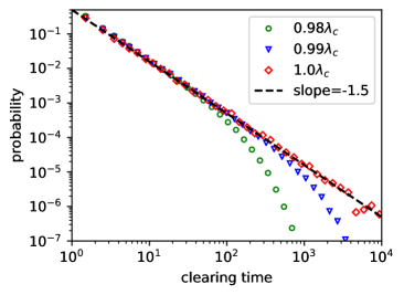
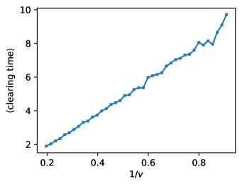
Figure 6: Simulation results for: (a) the clearing time probability for various $\lambda$ values, and (b) the average clearing time versus $1/v$ with $\lambda$ between $0.9\lambda_{c}$ and $0.98\lambda_{c}$, for a single elevator with capacity 50.

In the realistic case of $\lambda\mathrel{\raise 1.29167pt\hbox{$<$\kern-7.5pt\lower 4.30554pt\hbox{$\sim$}}}\lambda_{c}$, the average number of passengers waiting in the lobby will typically decreases by $C-\lambda T\equiv v$ in each cycle. We are primarily interested in the case where this systematic decrease is smaller than the random-walk step size, $\sqrt{\lambda T}$. The opposite limit is wasteful from a practical viewpoint, because it would correspond to a large excess of elevator capacity. Thus we treat the limit where the bias $v$ is small but negative during the start of the day rush. In this case $W_{n}$ undergoes a weakly biased random walk, again with a typical step size of $\sqrt{\lambda T}$. Now the distribution of clearing times will have the same $n^{-3/2}$ tail as in the critical case, but with a exponential cutoff due to the bias, which leads to the average clearing time scaling as $1/v$ [23]. This latter behavior is illustrated in Fig. 6(b).

4.3 The clearing probability

In addition to the clearing time, another useful indicator of the efficiency of the elevator system is the clearing probability $\mathbf{P}$, which we define as the probability that the lobby is cleared of all waiting passengers when the elevator leaves. We compute this probability in the current cycle in terms of the state of the system in the previous cycle. There are two cases that need to be considered: either the lobby was (a) cleared or (b) not cleared in the previous cycle. For case (a), we further require that the number of newly arriving passengers before the elevator next arrives does not exceed the elevator capacity $C$. In case (b), the number $W$ of remaining waiting passengers from last cycle plus the number of newly arriving passengers cannot exceed $C$. Under the assumption of a steady state, we have

$$\mathbf{P}=\mathbf{P}\,\mathcal{Q}(C|{\rm cleared})+(1-\mathbf{P})\sum_{W}R(W)\,\mathcal{Q}(C-W|{\rm not\,cleared})\,.$$ (11)

Here $\mathcal{Q}(X|\cdot)=\sum_{N}^{X}Q(N|\cdot)$ in the cumulative conditional probability that the number of new arriving passengers is $X$ or less, given that last cycle is either cleared or not cleared. The first term in (11) gives the contribution due to case (a) and the second term accounts for case (b). In this second term, $R(W)$ is the probability that $W$ passengers remain in the lobby after the elevator leaves, given that the lobby was not cleared in the previous cycle. Subsequently $C-W$ or fewer new passengers can arrive before the elevator next arrives so that the lobby will be cleared in the current cycle.

We now determine the factors in (11). We compute the stationary distribution $R(W)$ from the biased random-walk description of Sec. 4.2 for the number of people waiting in the lobby. For this random walk, the step size is $\delta x=\sqrt{\lambda T}$ and the bias is $v=C-\lambda T$. Since the unit of time in this random walk process is one elevator cycle, the single-step time is $\delta t=1$, from which the diffusion constant is $D=\delta x^{2}/(2\delta t)=\lambda T/2$. The stationary probability distribution of this biased random walk, subject to a absorbing boundary condition at $W=0$, is (see, e.g., [24])

$$R(W)=\frac{v}{D}\,e^{-vW/D}=2(\lambda_{c}/\lambda-1)e^{-2(\lambda_{c}/\lambda-1)W}\,,$$

with $v/D=(C-\lambda T)/(\lambda T/2)=2(\lambda_{c}/\lambda-1)$.

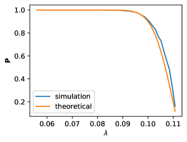
Figure 7: Comparison of the theoretical and simulation results for the clearing probability $\mathbf{P}$ for a single elevator with capacity 50.

We also replace the steady-state occupancy distribution $Q(N)$ by the infinite-capacity expression in Eq. (5). We further approximate $Q(N)$ by a Gaussian distribution with mean $N_{ss}$ and variance Var$(N)$ given in Eq. (9); this form compares well with our simulation results in Fig. 4. Thus the summation in (11) represents the cumulative of the convolution of an exponential and Gaussian distribution. This operation gives rise to the exponentially modified Gaussian distribution [25]. Thus we have

$$\sum_{W}R(W)\,\mathcal{Q}(C-W|{\rm not\,cleared})=\Psi(u,0,v)-e^{-u+v^{2}/2+\log[\Psi(u,v^{2},v)]}\,,$$

where the right-hand side is the cumulative of the exponentially modified Gaussian distribution [25], and $\Psi(u,0,v)$ is the cumulative Gaussian distribution itself, with arguments $u=2(\lambda_{c}/\lambda-1)(C-\lambda T)$, mean value $0$, and standard deviation $v=2\sqrt{\lambda T}(\lambda_{c}/\lambda-1)$.

Thus, Eq. (11), which determines the clearing probability $\mathbf{P}$ becomes

$$\mathbf{P}=\mathbf{P}\,\Psi(C,N_{ss},\sqrt{{\rm Var}(N_{ss})})+(1-\mathbf{P})\left\{\Psi(u,0,v)-e^{-u+v^{2}/2+\log[\Psi(u,v^{2},v)]}\right\}\,,$$ (12)

from which $\mathbf{P}$ can be immediately obtained. The resulting prediction for $\mathbf{P}$ closely matches our simulations shown in Fig. 7.

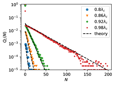
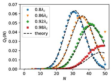
Figure 8: The distributions of (a) the number passengers still waiting in lobby, $Q_{L}(N)$, and (b) the number of passengers transported by elevator, $Q_{E}(N)$. Both cases correspond to a single elevator with capacity $C=50$.

For a finite capacity elevator, we can now determine both the number of passengers waiting in the lobby when the elevator departs and the number carried away by the elevator. Let $Q_{L}(N)$ and $Q_{E}(N)$ denote the distributions for these two quantities. If the lobby is cleared, there will be no passengers waiting, so that

$$Q_{L}(N)=\mathbf{P}\,\delta_{0,N}+2(1-\mathbf{P})\,(\lambda_{c}/\lambda-1)e^{-2(\lambda_{c}/\lambda-1)N}\,.$$ (13a)

If the lobby is not cleared, there will be necessarily $$C$$ passengers inside the elevator, so that

$$Q_{E}(N)=\mathbf{P}\,Q(N|N<C)+(1-\mathbf{P})\,\delta_{C,N}\,,$$ (13b)

where

$$Q(N|N<C)=\begin{cases}{\displaystyle{Q(N)}\Big{/}\;{\sum_{k=0}^{C}Q(k)}}&\qquad\text{if }N<C\,,\\[11.38109pt] 0&\qquad\text{otherwise}\,,\end{cases}$$

with $Q(N)$ the occupancy distribution in an infinite elevator system, which we can well approximate by a Gaussian distribution. Both these predictions match our theoretical expectations, as shown in Fig. 8.

We can now determine the distribution of times that an individual has to wait until an elevator arrives. We again need to treat two distinct cases. If an individual is accommodated within a single cycle, the time (s)he needs to wait will be the same as that in the infinite capacity limit; that is, $\mathcal{W}(t)$ in Eq. (6). If the person needs to wait for more then a cycle, her/his waiting time depends both on when (s)he arrives and the number of people already waiting for the elevator. The former attribute determines the waiting time within a cycle whereas the latter determines how many cycles must elapse before the person can be accommodated. Since the former time is uniformly distributed in $[0,T]$ for a fixed cycle time $T$, the total waiting time will be uniformly distributed in $[mT,(m+1)T]$, with $m$ a positive integer that is determined by the condition that the number of people $N$ already waiting in the lobby is in range of $[mC,(m+1)T]$. Equivalently, the number of people remaining in the lobby after an elevator departs must be in $[(m-1)C,mT]$.

Taking into account these two cases, the distribution of waiting times, $\mathcal{W}_{C}(t)$, for an elevator of capacity $C$, is formally given by

$$\mathcal{W}_{C}(t)=\mathbf{P}_{\mathcal{W}}\mathcal{W}(t)+\Theta(t-T)\,(1-\mathbf{P}_{\mathcal{W}})\;\frac{1}{T}\;\int_{(m-1)C}^{mC}Q_{L}(N)\,dN\,.$$ (14a)

Here $$\mathbf{P}_{\mathcal{W}} \Theta(\cdot) m=\text{floor}(t/T) \mathcal{W}(t) Q_{L}(N) Q_{L}(N) N$$ is the probability that an individual waits less than a single cycle time, denotes the Heaviside step function, , is the waiting time distribution (6) for an infinite-capacity elevator, and is the distribution of the number of people waiting in the lobby (given by Eq. (13a)) when the elevator leaves, and we have integrated over the allowable range of .

To make (14a) explicit, we need $\mathbf{P}_{\mathcal{W}}$. Naively, one might anticipate that $\mathbf{P}_{\mathcal{W}}$ should be the same as clearing probability $\mathbf{P}$. However, we need to account for another possibility: even when the lobby is not cleared in the current cycle, if the number $N$ of stranded passengers from previous cycle is less than $C$, then $C-N$ out of the $C$ passengers that are transported by the elevator in the current cycle will wait less than a single cycle. By including the additional term that accounts for this situation, the final result for $\mathbf{P}_{\mathcal{W}}$ is

$$\mathbf{P}_{\mathcal{W}}=\mathbf{P}+\int_{1}^{C}\frac{C-N}{C}\;Q_{L}(N)\,dN=\mathbf{P}+(1-\mathbf{P})\,\frac{2C(\lambda_{c}/\lambda-1)-e^{-2(\lambda_{c}/\lambda-1)C}+1}{2C(1-\lambda_{c}/\lambda)}\,,$$ (14b)

where we have substituted in the expression (13a) for $Q_{L}(N)$.

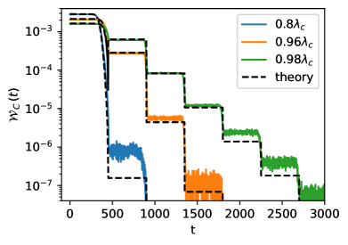
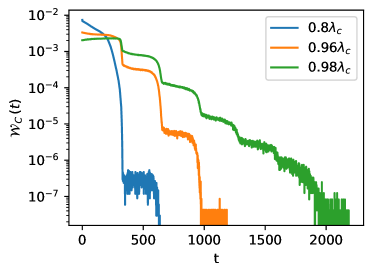
Figure 9: The distribution of times $\mathcal{W}_{C}(t)$ that a passenger waits until being able to board the elevator for: (a) for a single elevator of capacity $C=50$, and (b) for two elevators of capacity $C=25$.

Within each cycle, the waiting time distribution is Fermi-Dirac like, and multiple copies of these Fermi-Dirac-like distributions constitute the full waiting time distribution $\mathcal{W}_{C}(t)$ (Fig. 9(a)). Qualitatively, $\mathcal{W}_{C}(t)$ follows an overall exponential decay with time with a substructure that consists of these Fermi-Dirac steps. Since the elevator must be full if the lobby is not cleared, these steps beyond the first are much sharper than the first one. Figure 9(a) shows a close correspondence between our prediction (14) and the simulation data.

5 Multiple Finite-Capacity Elevators

Finally, we now turn to the realistic situation of a building that contains $k$ identical elevators, each of capacity $C$. We investigate two basic characteristics of the transport dynamics—the steady state and synchronization.

5.1 The steady state

Under the assumption that the elevators are uncorrelated, the steady-state criterion derived in Sec. 4.1 now becomes $\lambda T(C)\leq kC$. Again using Eq. $\eqref{TN}$ for $T(C)$, the steady-state condition is

$$\lambda\leq\lambda_{c}=\frac{k}{2\tau_{s}+2F/(C+1)}\,.$$ (15)

For elevators with capacity $C=20$ and using $\tau_{s}=2.5\,$sec, $F=100$, the steady-state criterion now gives $\lambda\leq 0.0689\,k$. As long as the elevators are uncorrelated, the overall transport capacity is simply proportional to the number of elevators.

It is instructive to estimate the number of elevators of capacity $C=20$ that are needed to service the start-of-day “rush” in an office building of 100 floors without having a pileup of passengers waiting in the lobby. We assume that each floor accommodates 100 people, so that $10^{4}$ people need to reach their offices at the start of a workday. With 20 people in each elevator, 500 elevator trips are needed. Each trip takes roughly 5 minutes for a total of 2500 elevator minutes. If the morning rush spans a two-hour period, these 2500 elevator minutes have to fit in a 120-minute window, which requires 21 elevators. These 21 elevators can accommodate a total passenger arrival rate of $\Lambda_{c}=21\,\lambda_{c}\approx 1.5$ passengers arriving per second and still remain in the steady state. This total arrival rate over a two-hour period also corresponds to accommodating all $10^{4}$ occupants of the building. If the elevators are uncorrelated, the time interval between successive events where an elevator reaches the ground floor should equal the single-elevator cycle time divided by the number of elevators, which is roughly 15 seconds. These numbers accord with common experience.

5.2 Synchronization

As passenger demand increases, it is not uncommon for a set of elevators to synchronize. This leads to the annoying feature that a large number of passengers build up in the lobby and then multiple elevators return to the lobby at nearly the same time. This clustering is analogous to what occurs in the bus-route model [16]. In this latter example, a circular bus route is serviced by multiple buses, with passengers arriving at a fixed rate at a set of bus stops. If a bus spends a time longer than usual at a stop because more passengers than usual are either loading or disembarking, the following bus will tend to catch up. Consequently, there is less time for passengers to accumulate at stops after the leading bus has departed. Since the number passengers waiting at stops will be less than average for the trailing bus, it will continue to catch up to the leading bus. If the trailing bus is allowed to pass the leading bus, the same instability arises in which there are fewer passengers than average waiting at each stop for the new trailing bus. Overall, this instability leads to an effective attraction between buses that tends to reduce their separation.

A similar instability occurs in a multi-elevator building when the arrival rate of passengers in the lobby is sufficiently large. Although each elevator runs on its own independent track, so that elevators can effectively “pass” each other, the same effective attraction between elevators occurs, which leads to the clustering of waiting passengers waiting in the lobby. To quantify this synchronization, let us first treat the much simpler case of deterministic dynamics and suppose that all elevators are already synchronized. Because of the deterministic dynamics, the number of waiting passengers in the lobby when all the elevators reach the ground floor equals $\lambda$ times the cycle time. We also suppose that $F_{\rm max}$ is deterministic and equal to its average value of $NF/(N+1)$, where $N$ is the number of passengers in each elevator (which is the same for each elevator). If the number of waiting passengers is large enough to trigger the movement of all $k$ elevators, then these elevators will again return at the same time in the next cycle. In turn, there will be a sufficient number of new waiting passengers to trigger the next cycle and lock the system in a synchronized state. Thus within deterministic dynamics, synchronization is locked in once it is achieved.

To trigger all $k$ elevators in the building, the number of waiting passengers should be greater than the capacity of $k-1$ elevators. That is,

$$\lambda T(N)>(k-1)C\,.$$

In this deterministic picture, the cycle time for all the elevators is $T(N)=2F_{\rm max}+2N\tau_{s}$, with $N=\eta C$ and $\eta$ in the range $(1-\frac{1}{k})$ to 1. At the lower limit case, $\lambda$ is just large enough that the number of waiting passengers, $\lambda T(N)$, just exceeds the capacity of $k-1$ elevators. At the upper limit, the number of waiting passengers completely fills all elevators. For simplicity we take $\eta=1$ henceforth. Using the expression $\lambda_{c}T=kC$, the lower bound for synchronization becomes

$$\lambda>\lambda_{c}\,(k-1)/k\,.$$ (16)

According to this deterministic picture, synchronization occurs in a narrow window of arrival rates that lies between $\lambda_{c}(k-1)/k$ and $\lambda_{c}$. This prediction is only approximate because we have not accounted for the randomness in the cycle times of each elevator.

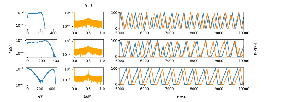
Figure 10: The inter-arrival time distribution $F(\Delta T)$ versus $\Delta T$ (left panels), the discrete Fourier transform $f(\omega)$ of the inter-arrival time series versus the normalized frequency $\omega/M$, where $M$ is the total number of intervals (middle panels), and representative late-time plots of the vertical positions of two elevators versus time for $\lambda=0.5\lambda_{c},0.8\lambda_{c}$, and $0.98\lambda_{c}$ for elevators with $C=50$

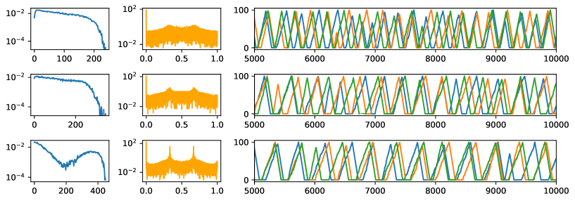
Figure 11: The same as in Fig. 10 for a three-elevator system.

Figure 12: The same as in Fig. 10 for a six-elevator system.

Illustrations of the vertical positions of each elevator versus time for a two-elevator, three-elevator, and six-elevator system are shown in the right panels of Figs. 10–12. Each row consists of data for the same value of $\lambda$. For these cases, the elevator trajectories tend to cluster when $\lambda\mathrel{\raise 1.29167pt\hbox{$>$\kern-7.5pt\lower 4.30554pt\hbox{$\sim$}}}0.9\lambda_{c}$. For $\lambda=0.8\lambda_{c}$, there are hints of synchronization for $k=2$ and $k=3$, but not for $k=6$. This behavior is expected from the deterministic picture of Eq. (16), in which synchronization requires $k\leq 5$ when $\lambda=0.8\lambda_{c}$.

A useful characteristic of the many-elevator system is the time $\Delta T$ between successive elevator arrivals. These inter-arrival times play an analogous role to successive cycle times in the single elevator system. When elevators become synchronized, there should be a repetitive pattern of a long time interval whose value is close to the single elevator cycle time, followed by $k-1$ short time intervals that correspond to the subsequent arrivals of nearly synchronized elevators (left panel of each figure). Because of the near periodicity of the elevators, it is helpful to study the Fourier transform of the ordered inter-arrival time series,

$$f(\omega)=\sum_{m=0}^{M-1}\Delta T_{m}\;e^{-2\pi im\omega/M}\,,$$

where $\Delta T_{m}$ is the $m^{\rm th}$ inter-arrival time and $M$ is the total number of time intervals in the dataset. In the synchronized state, this discrete Fourier transform should have $k-1$ peaks in addition to the component at zero frequency; this feature is illustrated in the middle panels of each figure.

Finally, we investigate the waiting time distribution for multiple elevators. We focus on the simplest case of the waiting-time distribution two elevators, and simulation results are shown in Fig. 9(b). The step-like form of the waiting-time distribution is a result of the synchronization of the two elevators. When the elevators become synchronized, we can treat one cycle of the two-elevator cluster as a single time unit for the biased random walk picture for the dynamics of number of passengers in the lobby. This leads to the long-time exponential decay of the waiting-time distribution, as in the single-elevator case. For times that are less than a single cycle, the waiting time distribution can be again deduced using (6) after replacing the cycle-time distribution $P(T)$ by the inter-arrival times distribution $F(\Delta T)$.

6 Concluding Comments

We investigated the transport of people by elevators in a tall building during the start-of-the-day operation within the framework of a minimal probabilistic model. For a single infinite-capacity elevator, we computed the expected time for one elevator cycle and the condition for a steady-state to arise. In this steady state, we determined the distribution of the elevator cycle times and occupancy distribution of the elevator. We constructed a rapidly converging iterative procedure that determined these distributions. The resulting distributions have well-defined peaks; thus fluctuations about the average are noticeable but do not overwhelm the dynamics.

For a single finite-capacity elevator, a new aspect of the dynamics is the clearing time, defined as the time interval between two successive events where all waiting passengers are accommodated by the elevator. We argued that this clearing time can be determined by invoking a random-walk picture for the number of passengers that remain in the lobby when the elevator departs. From this picture, we computed the average clearing time and its distribution. We also determined the distribution of the number of passengers who are stranded in the lobby when the elevator leaves and the number of passengers in the elevator. We then turned to the realistic situation of a fixed number of finite-capacity elevators. Again, we determined the condition for the steady state. Finally, we investigated the conditions under which a set of elevators will synchronize.

Our naive approach represents a small step in developing a physical understanding elevator transport. There are also many natural generalizations of the basic model that are worth considering within a our physics-based perspective. Perhaps the simplest is to study the situation where the cross-sectional area $A(h)$ of the building decreases with height $h$. A logical question now is: does there exist an optimal profile for $A(h)$ that minimizes the waiting time, but also optimizes available office space? Another relevant issue to investigate is that of elevator staging; that is, some fraction of the elevators services floors 0 through $F/2$ and another fraction services floors $F/2$ through $F$. Is this configuration better—in that the average waiting time and/or average total travel time is shorter—than two elevators that service all floors?

It should also be worthwhile to study the case of end-of-day operation, when occupants are leaving the building and nobody is entering. That is, passengers start their floor of occupancy and call for an elevator to take them to the ground floor. This case is not merely the time-reversed version of start-of-day operation and it would be interesting to understand the difference between these two cases.

ZFs Undergraduate Research Experience at the Santa Fe Institute was funded by the General Collaboration Agreement for the ASU-SFI Center for Biosocial Complex Systems. SRs research was partially supported by NSF grant DMR-1910736.

Appendix A Event-driven simulation algorithm

Our numerical results are based on an event-driven simulational approach, in which we only monitor the (variable) time interval for the next elevator to reach the ground floor. We describe our algorithm below, first for a single elevator of capacity $C$, and then for multiple elevators, each of the same capacity $C$.

One elevator

• If no passengers are waiting when an empty elevator reaches lobby, advance the time by an exponentially distributed random number $\delta t$ whose average value equals to the inter-arrival time between successive passengers. We then set $N=1$, since one new passenger is in the lobby.

• If $N\geq 1$ passengers are waiting when an elevator arrives, then:

  1. The waiting passengers enter the elevator until either all $N<C$ are accommodated or the elevator is full. The number of waiting passengers is decreased by $\text{min}(N,C)$.

  2. From the passenger destination floors, which are all chosen independently from a uniform distribution in $[1,F]$, determine the cycle time $T$ by setting $T=2F_{\rm max}\,+2N\tau_{s}$, where $F_{\rm max}$ is the maximum destination floor among the $N$ passengers and $\tau_{s}$ is randomly chosen from any well-behaved (i.e., no long tails) continuous distribution with mean value 2.5. In our simulations, we use a uniform distribution.

  3. Increment the time by $T$ and populate the lobby with $N$ new passengers, with $N$ chosen from a Poisson distribution with mean value $\lambda T$. The passengers currently in the elevator are erased.

  4. The elevator picks up the waiting passengers and a new cycle begins.

$k>1$ elevators

We need to now track the return time of each of the $k$ elevators and an event is defined by the return of the elevator with the shortest current return time.

• If no passengers are waiting when an empty elevator reaches the ground floor, advance the time by a random number $\delta t$ whose average value equals is the inter-arrival time between successive passengers, and then set $N=1$. Decrement the return times of all other elevators by $\delta t$.

• If $N\geq 1$ passengers are waiting when an elevator arrives, then:

  1. Passengers enter the elevator until either all $N<C$ passengers are accommodated or the elevator is full. The number of waiting passengers is decreased by $\text{min}(N,C)$.

  2. From the set of passenger destination floors, determine the return time $T$.

  3. Increment the time by $T_{\rm min}\equiv\text{min}\{T_{i}\}$, where $T_{i}$ is the current travel time of the $i^{\rm th}$ elevator to reach the lobby and $i$ runs from $1$ to $k$. Decrement the travel times of all other elevators by $T_{\rm min}$. Populate the lobby with $N$ new passengers, with $N$ chosen from a Poisson distribution with mean value $\lambda T_{\rm min}$.

  4. The elevator with the minimum return time picks up the waiting passengers and a new cycle begins.

  Note that loading an elevator, elevator travel, and elevator unloading are combined into a single event in this algorithm. Consequently, there is no possibility for a second elevator to arrive in the lobby during the time that one is currently loading passengers.

References

- [1] 2019 2018 Survey Report on the number of elevators installed URL https://www.n-elekyo.or.jp/about/elevatorjournal/pdf/Journal26_01_20191218.pdf
- [2] 2017 Elevator Report URL https://www1.nyc.gov/assets/buildings/html/elevator_report_2017.html
- [3] 2020 Overview of the Latest Regulatory Control For Lift and Escalator Safety in Hong Kong URL https://cibse.org.hk/wp-content/uploads/2020/01/Overview-of-the-latest-regulatory-control-for-lift-and-escalator-safety-in-Hong-Kong-EMSD.pdf
- [4] Pepyne D L and Cassandras C G 1997 IEEE transactions on control systems technology 5 629–643
- [5] Hikihara T and Ueshima S 1997 IEICE Transactions on Fundamentals of Electronics, Communications and Computer Sciences 80 1548–1533
- [6] Schlemmer M and Agrawal S K 2002 IEEE transactions on control systems technology 10 105–111
- [7] Bertsekas D P and DP B 1976
- [8] Bartz-Beielstein T, Preuss M and Markon S 2005 Validation and optimization of an elevator simulation model with modern search heuristics Metaheuristics: Progress as Real Problem Solvers (Springer) pp 109–128
- [9] Siikonen M L 1993 Simulation 61 257–267
- [10] Lee Y, Kim T S, Cho H S, Sung D K and Choi B D 2009 Mathematical and Computer modelling 49 423–431
- [11] Barney G and Al-Sharif L 2015 Elevator traffic handbook: theory and practice (Routledge)
- [12] Al-Kodmany K 2015 Buildings 5 1070–1104 ISSN 2075-5309 URL https://www.mdpi.com/2075-5309/5/3/1070
- [13] Pöschel T and Gallas J A 1994 Physical Review E 50 2654
- [14] Nagatani T 2003 Physica A: Statistical Mechanics and its Applications 326 556–566
- [15] Nagatani T 2004 Physica A: statistical mechanics and its applications 333 441–452
- [16] O’Loan O, Evans M R and Cates M E 1998 Physical Review E 58 1404
- [17] Hall H and Zambelli E 1958 Journal of Jet Propulsion 28 463–465
- [18] Burghes D N 1974 International Journal of Mathematical Education in Science and Technology 5 3–10 (Preprint https://doi.org/10.1080/0020739740050101) URL https://doi.org/10.1080/0020739740050101
- [19] Gumbel E J 2012 Statistics of extremes (Courier Corporation)
- [20] Galambos J 1978 The asymptotic theory of extreme order statistics Tech. rep.
- [21] 2020 Elevator URL https://en.wikipedia.org/wiki/Elevator
- [22] Weiss N A 2006 A course in probability (Addison-Wesley)
- [23] Redner S 2001 A guide to first-passage processes (Cambridge University Press)
- [24] Crank J 1979 The mathematics of diffusion (Oxford university press)
- [25] 2020 Exponential modified Gaussian distribution URL https://en.wikipedia.org/wiki/Exponentially_modified_Gaussian_distribution
- [26] 2019 Willis Tower History & Facts URL https://www.willistower.com/history-and-facts