Self-Explaining Structures Improve NLP Models

Abstract

Existing approaches to explaining deep learning models in NLP usually suffer from two major drawbacks: (1) the main model and the explaining model are decoupled: an additional probing or surrogate model is used to interpret an existing model, and thus existing explaining tools are not self-explainable; (2) the probing model is only able to explain a model’s predictions by operating on low-level features by computing saliency scores for individual words but are clumsy at high-level text units such as phrases, sentences, or paragraphs.

To deal with these two issues, in this paper, we propose a simple yet general and effective self-explaining framework for deep learning models in NLP. The key point of the proposed framework is to put an additional layer, as is called by the interpretation layer, on top of any existing NLP model. This layer aggregates the information for each text span, which is then associated with a specific weight, and their weighted combination is fed to the softmax function for the final prediction.

The proposed model comes with the following merits: (1) span weights make the model self-explainable and do not require an additional probing model for interpretation; (2) the proposed model is general and can be adapted to any existing deep learning structures in NLP; (3) the weight associated with each text span provides direct importance scores for higher-level text units such as phrases and sentences. We for the first time show that interpretability does not come at the cost of performance: a neural model of self-explaining features obtains better performances than its counterpart without the self-explaining nature, achieving a new SOTA performance of 59.1 on SST-5 and a new SOTA performance of 92.3 on SNLI.

1 Introduction

A long-term criticism against deep learning models is the lack of interpretability Simonyan et al. (2013); Bach et al. (2015a); Montavon et al. (2017); Kindermans et al. (2017). The black-box nature of neural models not only significantly limits the scope of applications of deep learning models (e.g., in biomedical or legal domains), but also hinders model behavior analysis and error analysis.

To enhance neural models’ interpretability, various approaches to rationalize neural models’ predictions have been proposed (details see Section 2). Existing interpretation models have two major drawbacks. Firstly, they are not self-explainable and require a probing model to be additionally built to interpret the original model. Building the probing model is not only an additional burden, but more importantly, the intrinsic decoupling nature of the two models makes the probing model only able to provide approximate interpretation results. Take the gradient-based saliency model Simonyan et al. (2013); Li et al. (2015); Selvaraju et al. (2017) as an example, the derivative of the target probability (or the logit) w.r.t. the input dimensions is only an approximate feature weight in the first-order Taylor expansion, with all higher order items omitted.

Secondly, interpretation models mostly focus on learning word-level importance scores assigned by the the main model and are hard to be adapted to higher-level text units such as phrases, sentences, or paragraphs. A straightforward way to compute the saliency score for a phrase or a sentence could be averaging the scores for its constituent words. Unfortunately, this over-simplified strategy is inadequate to capture the semantic composition in language, which involves multiple layers of highly non-linear operations in neural nets, and can thus result in high risk of misinterpretation. As pointed by Murdoch et al. (2018), interpreting neural net predictions should go beyond word level.

We raise the following question: what makes a good interpretation method for NLP? Firstly, the method should be self-explainable and no additional probing model is needed. Secondly, the model should offer precise and clear saliency scores for any level of text units. Thirdly, the self-explainable nature does not tradeoff performances.

Towards these three purposes, in this paper, we propose a self-explainable framework for deep neural models in the context of NLP. The key point of the proposed framework is to put an additional layer, as is called the interpretation layer on top of any existing NLP model, and this layer aggregates the information for all (i.e., $\mathcal{O}(n^{2})$) text spans. Each text span is associated with a specific weight, and their weighted combination is fed to the softmax function for the final prediction. The proposed structure offers following advantages: (1) the model is self-explainable: the interpretation layer is trained along with the objective, with no probing model needed. Weights at the interpretation layer can directly be used as saliency scores for corresponding text spans; (2) since the saliency score for any text span can be straightforwardly derived from the interpretation layer, the model offers direct, precise and clear saliency scores for any level of text units beyond word level. (3) the interpretation layer collects information for each text span in the form of representations, and forwards the weighted sum to the final prediction layer. Therefore, no additional information is incorporated, nor any information is lost at the interpretation layer. This makes the model not come at the cost of performances.

The proposed framework is general, and can be adapted to any prevalent deep learning structure in NLP. We show that the proposed framework (1) offers clear model interpretations; (2) facilitates error analysis; (3) can help downstream NLP tasks such as adversarial example generation; and (4) most importantly, for the first time proves that self-explainable nature does not come at the cost of performances, but rather, leads to better results in NLP, achieving a new SOTA performance of 59.1 on SST-5 and a new SOTA performance of 92.3 on SNLI.

2 Related Work

Rationalizing model predictions is of growing interest (Ribeiro et al., 2016; Shrikumar et al., 2017; Bach et al., 2015b; Kindermans et al., 2017; Montavon et al., 2017; Schwab and Karlen, 2019; Arrieta et al., 2020). In NLP, approaches to interpret neural models include extracting pieces of input text, called “rationales”, as justifications to model predictions (Lei et al., 2016; Chang et al., 2019; DeYoung et al., 2020; Jain et al., 2020), studying the efficacy and dynamics of hidden states in recurrent networks (Karpathy et al., 2015; Shi et al., 2016; Greff et al., 2016; Strobelt et al., 2016), and applying variants of the attention mechanism (Bahdanau et al., 2014) to interpret model behaviors Jain and Wallace (2019); Serrano and Smith (2019); Wiegreffe and Pinter (2019); Vashishth et al. (2019); Rogers et al. (2020). Lei et al. (2016) proposed to extract text snippets as model explanations. Rajani et al. (2019) collected human rationales for commonsense reasoning. Other works (Chen et al., 2019; Lehman et al., 2019; Chai et al., 2020) trained independent models to extract supporting sentences as auxiliary guidelines for downstream tasks. Using attentions as a tool for model interpretation, Ghaeini et al. (2018) visualized attention heatmaps to understand how natural language inference models build interactions between two sentences; Vig and Belinkov (2019); Tenney et al. (2019); Clark et al. (2019); Htut et al. (2019) analyzed the attention structures by plotting heatmaps, and found that meaningful linguistic patterns exist in different heads and layers. Despite the interpretability the attention mechanism offers, Serrano and Smith (2019); Jain and Wallace (2019) observed the highly inconsistency between attentions and predictors, and suggested that attentions should not be treated as justification for a decision.

Saliency methods are widely used in computer vision (Simonyan et al., 2013; Zeiler and Fergus, 2014; Springenberg et al., 2014; Adler et al., 2018; Datta et al., 2016; Srinivas and Fleuret, 2019) and NLP Denil et al. (2015); Li et al. (2015, 2016); Arras et al. (2016); Ebrahimi et al. (2017); Feng et al. (2018); Meng et al. (2020) for model interpretation. The key idea is to find the salient features responsible for a model’s prediction. Simonyan et al. (2013); Srinivas and Fleuret (2019) visualized the contributions of input pixels by compute the derivatives of the label logit in the output layer with respect to the input pixel. Adler et al. (2018); Datta et al. (2016) explained neural models by perturbing different parts of the input, and compared the performance change in downstream tasks to measure the importance of perturbed features. In the context of NLP, Denil et al. (2015) used saliency maps to identify and extract task-specific salient sentences from documents to maximally preserve document topics and semantics; Li et al. (2015) visualized word-level saliency maps to understand how individual words affect model predictions; Ebrahimi et al. (2017) crafted white-box adversarial examples to find the most salient text-editing operations (flip, insertion and deletion) to trick models by computing derivatives w.r.t. these editing operations; Meng et al. (2020) combined the saliency method and the influence function (Koh and Liang, 2017) to interpret model predictions from both learning history and inputs.

Our work is inspired by Melis and Jaakkola (2018), which achieves “self-explaining” by jointly training a deep learning model and a linear regression model with human-interpretable features. It is worth noting that the model in Melis and Jaakkola (2018) still requires a surrogate model, i.e., the linear regression model with human-interpretable features. Instead, the proposed framework does not require a surrogate model. Our work is also inspired by Selvaraju et al. (2017) in computer vision, which computes the gradient w.r.t. feature maps of the high-level convolutional layer to obtain high-level saliency scores.

3 The Self-Explaining Framework

3.1 Notations

Given an input sequence $\bm{x}=\{x_{1},x_{2},...,x_{N}\}$, where $N$ denotes the length of $\bm{x}$. Let $\bm{x}(i,j)$ denote the text span starting at index $i$, ending at index $j$, where $\bm{x}(i,j)=\{x_{i},x_{i+1},...,x_{j-1},x_{j}\}$. We wish to predict the label $y$ for $\bm{x}$ based on $p(y|\bm{x})$. Let $V$ denote vocabulary size, and word representations are stored in $\bm{W}\in\mathbb{R}^{V\times D}$. The input $\bm{x}$ is associated with the label $y\in\mathcal{Y}$.

3.2 Model

For illustration purposes, we use transformers Vaswani et al. (2017) as the backbone to show how the proposed framework works. The framework can be easily extended to other models such as BiLSTMs or CNNs. An overview of the proposed model is shown in Figure 1.

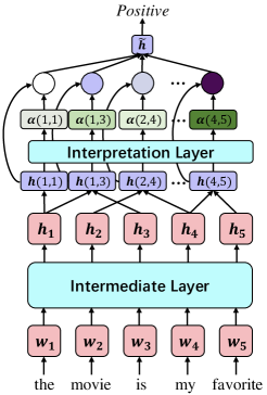
Figure 1: An overview of the proposed model.

Input Layer Similar to standard deep learning models in NLP, the input layer for the proposed model consists of the stack of word representations for words in the input sequence, where $x_{t}$ is represented as a $D$-dimensional vector $\bm{W}[x_{t},:]$.

Intermediate Layer On top of the input layer are the $K$ encoder stacks, where each stack consists of multi-head attentions, layer normalization and residual connections. The representation for $k$-th layer at position $t$ is denoted by $\bm{h}_{t}^{k}\in\mathbb{R}^{1\times D}$. Specially, the presentation for the last layer at position $t$ is denoted by $\bm{h}_{t}^{K}\in\mathbb{R}^{1\times D}$.

Span Infor Collecting Layer (SIC) To enable direct measurement for saliency of an arbitrary text span, we place a Span Infor Collecting Layer on top of intermediate layer. For an arbitrary text span $\bm{x}(i,j)$, we first obtain a dense representation $\bm{h}(i,j)$ to represent $\bm{x}(i,j)$, and $\bm{h}(i,j)$ needs to contain all semantic and syntactic information stored in $\bm{x}(i,j)$. Concretely, $\bm{h}(i,j)$ is obtained by taking the representation for the starting index at the last intermediate layer $\bm{h}^{K}_{i}$, and the representation for the ending index $\bm{h}^{K}_{j}$:

$$\bm{h}(i,j)=F(\bm{h}^{K}_{i},\bm{h}^{K}_{j})$$ (1)

where $F$ denotes the mapping function, which be FFN or other forms. The details of $F$ will be discussed in section 3.3. The strategy of using the starting and ending representations to represent a text span has been used in many recent works on span-level features in texts Li et al. (2019); Joshi et al. (2020); Wu et al. (2019). The SIC layer iterates over all text spans, and collects $\bm{h}(i,j)$ for all $i\in[1,N]$, $j\in[i,N]$, with the complexity being $\mathcal{O}(N^{2})$.

Interpretation Layer The interpretation layer aggregates information from all text spans $\bm{h}(i,j)$: this is achieved by first assigning weights $\alpha(i,j)$ to each span $\bm{x}(i,j)$ and combing these representations using weighted sum. The weight $\alpha(i,j)$ can be obtained by first mapping $\bm{h}(i,j)$ to a scalar, and then normalizing all $\alpha(i,j)$:

$$o(i,j) =\hat{\bm{h}}^{\top}\bm{h}(i,j)$$ (2)

$$\alpha(i,j) =\frac{\exp(o(i,j))}{\sum_{i\in[1,N],j\in[i,N]}\exp(o(i,j))}$$

where $\hat{\bm{h}}\in\mathbb{R}^{1\times D}$. The output $\tilde{\bm{h}}\in\mathbb{R}^{1\times D}$ from the interpretation layer is the weighted average of all span representations:

$$\tilde{\bm{h}}=\sum_{i\in[1,N],j\in[i,N]}\alpha(i,j)\bm{h}(i,j)$$ (3)

Output Layer Similar to the standard setup, the output layer of the proposed framework is the probability distribution over labels using the softmax function:

$$p(y|\bm{x})=\frac{\bm{u}_{y}^{\top}\tilde{\bm{h}}}{\sum_{y\in\mathcal{Y}}\bm{u}_{y}^{\top}\tilde{\bm{h}}}$$ (4)

where $\bm{u}_{y}\in\mathbb{R}^{D\times 1}$. As can be seen, $\alpha(i,j)$ measures how much $\bm{x}(i,j)$ contributes to the final representation $\tilde{\bm{h}}$, and thus indicates the importance of the text span $\bm{x}(i,j)$. The proposed strategy is similar to gradient-based interpretation methods Simonyan et al. (2013); Li et al. (2015). Using the chain rule, we have

$$\frac{\partial p(y|\bm{x})}{\partial\bm{h}(i,j)}=\frac{\partial p(y|\bm{x})}{\partial\tilde{\bm{h}}}\frac{\partial{\tilde{\bm{h}}}}{\partial{\bm{h}(i,j)}}$$ (5)

$$=\frac{\partial p(y|\bm{x})}{\partial\tilde{\bm{h}}}\left[\alpha(i,j)+\bm{h}(i,j)\frac{\partial{\alpha(i,j)}}{\partial\bm{h}(i,j)}\right]$$

Omitting the second part, ${\partial p(y|\bm{x})}/{\partial\tilde{\bm{h}}}$ is approximately in proportion to $\alpha(i,j)$. There is also a key advantage of the proposed framework over existing gradient-based interpretation methods, where the interpretation layer allows gradients to be straightforwardly computed with respect to an arbitrary text span. This is not feasible for vanilla gradient-based methods: because of the highly entanglement of neural networks, it’s impossible to filter out the information of a specific text span from intermediate layers. Only gradients w.r.t. the input layer offers non-disentangling saliency scores, making the model only able to perform word-level explanations.

3.3 Efficient Computing

A practical issue with Eq.1 is the computation cost. If $F$ takes the form of FFN, the computational complexity for one single text span is $\mathcal{O}(D^{2})$, leading to a final complexity of $\mathcal{O}(N^{2}D^{2})$ if all spans are iterated over. This is computationally unaffordable for long texts. Towards efficient computations, we propose that $F$ takes the following form:

$$F(\bm{h}_{i},\bm{h}_{j})=\tanh[\bm{W}(\bm{h}_{i},\bm{h}_{j},\bm{h}_{i}-\bm{h}_{j},\bm{h}_{i}\otimes\bm{h}_{j})]$$ (6)

where $\bm{W}=[\bm{W}_{1},\bm{W}_{2},\bm{W}_{3},\bm{W}_{4}]$, $\bm{W}_{i}\in\mathbb{R}^{D\times D}$. $\otimes$ denotes the pairwise dot between two vectors. Elements in $(\bm{h}_{i},\bm{h}_{j},\bm{h}_{i}-\bm{h}_{j},\bm{h}_{i}\otimes\bm{h}_{j})$ respectively captures concatenation, element-wise difference and element-wise closeness between the two vectors, the strategy of which is been used in recent work to model interactions between two semantic representations Mou et al. (2015); Seo et al. (2016).

In Eq.6, $\bm{W}_{1}\bm{h}_{i}$, $\bm{W}_{2}\bm{h}_{j}$, $\bm{W}_{3}\bm{h}_{i}$ and $\bm{W}_{3}\bm{h}_{j}$ can be computed in advance for all $i$ and $j$, leading to a computational complexity of $\mathcal{O}(ND)$. For $\bm{W}_{4}\bm{h}_{i}\otimes\bm{h}_{j}$, it can be factorized as $\sqrt{\bm{W}_{4}}\bm{h}_{i}\otimes\sqrt{\bm{W}_{4}}\bm{h}_{j}$, with each of the two parts being computed in advance. The final computational complexity of $\bm{W}(\bm{h}_{i},\bm{h}_{j},\bm{h}_{i}-\bm{h}_{j},\bm{h}_{i}\otimes\bm{h}_{j})$ is thus $\mathcal{O}(ND)$. The element-wise tanh operation for all $N^{2}$ spans leads to a cost of $\mathcal{O}(N^{2}D)$, giving a complexity of $\mathcal{O}(N^{2}D)+\mathcal{O}(ND)=\mathcal{O}(N^{2}D)$ for the SIC layer, which significantly cuts the cost. The computational cost for the interpretation layer, which requires the dot product between $\hat{\bm{h}}$ and all $\bm{h}(i,j)$, is also $\mathcal{O}(N^{2}D)$, leading to the final computational complexity $\mathcal{O}(N^{2}D)$. In this way, we reduce the computation cost from $\mathcal{O}(N^{2}D^{2})$ to $\mathcal{O}(N^{2}D)$.

3.4 Training

The training objective is the standard cross entropy loss. An additional regularization on $\bm{\alpha}$ is needed: the model should only focus on a very small number of text spans. We thus wish the distribution of $\bm{\alpha}$ to be sharp. We thus propose the following training objective:

$$\mathcal{L}=\log p(y|\bm{x})+\lambda\sum_{i,j}\alpha^{2}(i,j)$$ (7)

which uses $\sum_{i,j}\alpha^{2}(i,j)$ as the regularizer. Under the constraint of $\sum_{i,j}\alpha(i,j)=1$, $\sum_{i,j}\alpha^{2}(i,j)$ achieves the highest value with one element of $\alpha$ being 1 and the rest being 0, and the lowest value if all $\alpha(i,j)$ have the same value. The model can be trained in an end-to-end fashion.

4 Evaluation

We would like an automatic evaluation method that is both flexible in evaluating the quality of model explanations under any task and dataset, and able to offer the ability of accurately reflecting the faithfulness of model explanations, i.e., the extracted rationales ought to semantically influence the model’s prediction for the same instance, as suggested by DeYoung et al. (2020).

Intuitively, if extracted rationales can faithfully represent, in other words, be equivalent to, their corresponding text inputs with respect to model predictions, the following should hold: (1) a model trained on the original inputs should perform comparably well when tested on the extracted rationales; (2) a model trained on the extracted rationales should perform comparably well when tested on the original inputs; (3) a model trained on the extracted rationales should perform comparably well when tested on other extracted rationales. Higher performances on these three aspects indicate more faithful extracted rationales, and consequently better interpretation models. These strategies are inspired by Lei et al. (2016), who trained a rationale generator to extract text pieces as explanations for different sentiment aspects for the task of sentiment analysis, achieving high precision based on sentence-level aspect annotations.

More formally, we use full to refer to the situation of training or testing a model on the original texts, and span to refer to the situation of training or testing a model on the extracted rationales. By denoting the original full dataset by $D_{\text{train}}$, $D_{\text{dev}}$ and $D_{\text{test}}$, and the newly constructed rationale-based dataset by $D^{\prime}_{\text{train}}$, $D^{\prime}_{\text{dev}}$ and $D^{\prime}_{\text{test}}$, the settings described above are as follows:

• FullTrain-SpanTest: The model is trained on $D_{\text{train}}$ and tested on $D^{\prime}_{\text{test}}$, with hyperparameters selected on $D_{\text{dev}}$.

• SpanTrain-FullTest: The model is trained on $D^{\prime}_{\text{train}}$ and tested on $D_{\text{test}}$, with hyperparameters selected on $D^{\prime}_{\text{dev}}$.

• SpanTrain-SpanTest: The model is trained on $D^{\prime}_{\text{train}}$ and tested on $D^{\prime}_{\text{test}}$, with hyperparameters selected on $D^{\prime}_{\text{dev}}$.

To construct the new rationale-based dataset, we train a rationale-extraction model on $D_{\text{train}}$ to extract rationales from the original text in $D_{\text{train}}$, $D_{\text{dev}}$ and $D_{\text{test}}$, and then replace the original full input text with the corresponding extracted rationales, with the labels remaining unchanged.

It is also worthing that the proposed three evaluation metrics are far from perfect: the system can be gamed if the extracted plan is just the same as the original span. The proposed evaluations thus need to be combined with other evaluations for complement.

5 Experiments

5.1 Tasks and Datasets

We conduct experiments on three NLP tasks: text classification on the SST-5 dataset Socher et al. (2013), natural language inference on the SNLI dataset Bowman et al. (2015) and machine translation on the IWSLT2014 En$\rightarrow$De dataset. Please refer to the appendix section for descriptions of the three datasets and training details.

For text classification and natural language inference, we use RoBERT (Liu et al., 2019b) as the model backbone. For reference purposes, we also train a self-explaining model with $\bm{\alpha}$ set to be uniform, i.e., $\alpha(i,j)=1/M$, where $M$ is the total number of text spans. This model is denoted by AvgSelf-Explaining. For neural machine translation, we use the Transformer-base (Vaswani et al., 2017) model for evaluation.

Model	Accuracy$\uparrow$
SST-5
BCN+SuBiLSTM+CoVe (Brahma, 2018)	56.2
BERT-base (Cheang et al., 2020)	54.9
BERT-large (Cheang et al., 2020)	56.2
SentiBERT (Yin et al., 2020)♭	56.9
SentiLARE (Ke et al., 2020)♭†	58.6
1-2 RoBERTa-base+AvgSelf-Explaining	56.2
RoBERTa-base (Liu et al., 2019b)	56.4
RoBERTa-base+Self-Explaining	57.8 (+1.4)
1-2 RoBERTa-large (Liu et al., 2019b)	57.9
RoBERTa-large+Self-Explaining	59.1 (+1.2)
SNLI
BERT-base (Zhang et al., 2019)	89.2
BERT-large (Zhang et al., 2019)	90.4
SJRC (Zhang et al., 2019)†	91.3
NILE (Kumar and Talukdar, 2020)♭	91.5
MT-DNN (Liu et al., 2019a)†	91.6
SemBERT (Zhang et al., 2020b)†	91.9
CA-MTL (Pilault et al., 2020)♮†	92.1
1-2 RoBERTa-base+AvgSelf-Explaining	90.8
RoBERTa-base (Liu et al., 2019b)	90.7
RoBERTa-base+Self-Explaining	91.7 (+1.0)
1-2 RoBERTa-large (Liu et al., 2019b)	91.4
RoBERTa-large+Self-Explaining	92.3 (+0.9)

Table 1: Performances of different models on the SST-5 and SNLI datasets. ^♭ denotes using RoBERTa-base as the model backbone, ^♮ denotes using RoBERTa-large as the model backbone, and ^† denotes using external training resources.

Model	BLEU$\uparrow$
IWSLT 2014 En$\rightarrow$De
Transformer-base (Vaswani et al., 2017)	28.4
Transformer-base+Self-Explaining	28.9

Table 2: Performances of different models on the IWSLT 2014 En$\rightarrow$De dataset.

5.2 Main Results

Table 1 shows the results for the SST-5 and SNLI datasets, and Table 2 shows the results for IWSLT 2014 En$\rightarrow$De. We can see from the tables that the proposed Self-Explaining method significantly boosts performances over strong RoBERTa baselines on SST-5 and SNLI. Using RoBerta-large, we achieve a new SOTA performance of 59.1 on SST-5 and a new SOTA performance of 92.3 on SNLI. A surprising observation is that in spite of using the SIC layer and the interpretation layer, AvgSelf-Explaining still underperforms RoBERTa, which indicates that the learned attention weights $\bm{\alpha}$ are important for model performances.

5.3 Interpretability Evaluation

We compare our proposed Self-Explaining model with the following three widely used interpretation models:

• AvgGradient: The method of averaging word saliency scores within a text span (Li et al., 2015; Feng et al., 2018). The saliency score of a word $w$ is computed as the derivative of the probability of the ouput label with respect to the word embedding: $s_{y}(w)=\|\nabla_{\bm{w}}p(y|\bm{x})\|_{1}$, where $p(y|\bm{x})$ is the predicted probability of the ground-truth label $y$, $\bm{w}$ is the corresponding word embedding of word $w$ and $\|\cdot\|_{1}$ is the L1 norm. We take the average of saliency scores of all words within a text span as the span-level saliency score. We select the span with the highest span-level saliency score as the rationale.

• AvgAttention: The method of averaging attention scores within a text span (Vig and Belinkov, 2019; Tenney et al., 2019; Clark et al., 2019). The attention score for each word $w$ is the normalized attentive probability of the special token [CLS] with respect to word $w$ in the last intermediate layer. We take the average of attention scores of all words within a text span as the span-level attention score. The span with the highest span-level attention score is selected as the rationale.

• Rationale: The rationale extraction model proposed by Lei et al. (2016). One encoder is used to encode input texts into representative features, and one generator is used to extract text spans as rationales. These two models are jointly trained to minimize the expected cost function using the REINFORCE algorithm (Williams, 1992).

All models use RoBERTa (Liu et al., 2019b) as the backbone and are trained separately for comparison.

Results are shown in Table 4. For all the three setups FullTrain-SpanTest, SpanTrain-FullTest and SpanTrain-SpanTest, we can observe that the proposed Self-Explaining outperforms other interpretation methods by a large margin on both SST-5 and SNLI. On SST, Self-Explaining outperforms Rationale by +3.2, +5.0 and +6.7 respectively for the F-S, S-F and S-S setup. On SNLI, Self-Explaining outperforms Rationale by +3.5, +10.0 and 7.3 respectively for the F-S, S-F and S-S setup. Comparing AvgGradient, AvgAttention and Rationale, we can see that there is no method that shows consistent superiority to the other two. For example, Rationale outperforms AvgGradient and AvgAttention under the F-S and S-F setup, but underperforms AvgGradient under the S-S setup. Instead, Self-Explaining consistently achieves significantly better results compared to all baselines under all setups. These results demonstrate the better interpretability of the proposed Self-Explaining method.

Model	IOU F1	Token F1
Movie Review
AvgGradient	0.075	0.175
AvgAttention	0.067	0.142
Rationale (Lei et al., 2016)	0.132	0.281
Self-Explaining	0.152	0.314
SNLI
AvgGradient	0.251	0.349
AvgAttention	0.301	0.435
Rationale (Lei et al., 2016)	0.381	0.459
Self-Explaining	0.454	0.571

Table 3: Performances of different models on Movie Review and SNLI of the ERASER benchmark.

Model	F-S	S-F	S-S
SST-5
AvgGradient	34.1	45.6	36.9
AvgAttention	32.5	40.6	35.8
Rationale (Lei et al., 2016)	35.2	49.9	36.2
Self-Explaining	38.4	54.9	42.9
SNLI
AvgGradient	70.7	74.5	73.1
AvgAttention	64.5	72.5	70.4
Rationale (Lei et al., 2016)	71.0	78.5	71.9
Self-Explaining	74.5	88.5	79.2

Table 4: Performances of different models on the three evaluation methods defined in Section 4. “F” refers to Full and “S” refers to Span. Accuracy is reported in each cell.

Label	Model	Text
Very Negative	(1)	this overproduced and generally disappointing effort isn’t likely to rouse the rush hour crowd
	(2)	this overproduced and generally disappointing effort isn’t likely to rouse the rush hour crowd
	(3)	this overproduced and generally disappointing effort isn’t likely to rouse the rush hour crowd
Negative	(1)	However, it lacks grandeur and that epic quality often associated with Stevenson’s tale as well as with earlier Disney efforts
	(2)	However, it lacks grandeur and that epic quality often associated with Stevenson’s tale as well as with earlier Disney efforts
	(3)	However, it lacks grandeur and that epic quality often associated with Stevenson’s tale] as well as with earlier Disney efforts
Negative	(1)	Though everything might be literate and smart, it never took off and always seemed static
	(2)	Though everything might be literate and smart, it never took off and always seemed static
	(3)	Though everything might be literate and smart, it never took off and always seemed static
Very Positive	(1)	One of the greatest family-oriented, fantasy-adventure movies ever
	(2)	One of the greatest family-oriented, fantasy-adventure movies ever
	(3)	One of the greatest family-oriented, fantasy-adventure movies ever

Table 5: Examples of correctly classified texts and the corresponding extracted text spans by different models. (1): Self-Explaining; (2): AvgGradient; (3): AvgAttention.

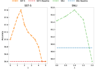
Figure 2: Performances of the proposed model with respect to different values of $\lambda$. Accuracy is reported for comparison.

5.4 The Effect of $\lambda$

We would like to explore the effect of $\lambda$ in the additional regularization term in Eq.7. A larger $\lambda$ has a stronger effect on sharpening the distribution of $\bm{\alpha}$, leading to the preference to a small fraction of text spans. Intuitively, a reasonable value of $\lambda$ is crucial for model performances: too small $\lambda$ means the selected text spans are not confident enough to support model predictions, while too large $\lambda$ means the model only attends to a single text span for its prediction. The former may cause over-numbered selected text spans, which incurs more noise for model predictions. The latter may force the model the attend to a single span that is not important for predictions. Therefore, a sensible $\lambda$ should be neither too small nor too large, balancing the number of attended text spans.

Figure 2 shows the results. As we can see from the figure, $\lambda=1.5$ leads to the best result on SST-5 and $\lambda=1.0$ gives the best result on SNLI, significantly outperforming models with small $\lambda$ and large $\lambda$, as well as the baseline. As the value of $\lambda$ keeps increasing, the performance drastically drops. When $\lambda=5.0$ for SST-5 and $\lambda=2.0$ for SNLI, the accuracies are respectively 56.4 and 90.3, even underperforming baselines without self-explaining structures. To our surprise, though the model performance with $\lambda=0$ is worse than the best model with $\lambda=1.5$ and $\lambda=1.0$, it still achieves better results compared to baselines (57.0 vs. 56.4 on SST-5 and 91.4 vs. 90.7 on SNLI). This observation verifies that the proposed method can actually improve NLP models in terms of both performance and interpretability.

True	Predicted	Text
Negative	Positive	the story is naturally poignant, but first - time screen-writer paul pender overloads it with sugary bits ofbusiness
Negative	Neutral	a well acted and well intentioned snoozer
Negative	Positive	george, hire a real director and good writers forthe next installment, please
Positive	Negative	It ’s like a poem
Positive	Very Negative	There isn’t a weak or careless performance amongst them

Table 6: Examples of mis-classified texts and the corresponding extracted text spans.

Label	Text
Positive $\hookrightarrow$Negative	In the film, Lumumba, we see the faces behind the monumental shift in the Congo’s history after it is reclaimed from the Belgians, and we see the motives behind those men into whose hands the raped and starving country fell. Lumumba is not a movie for the hyper masses; it demands the attention of its viewers with raw, truthful acting and intricate, packed dialogue. Little of the main plot is shown through action, it relies almost solely on words, but there is a recurring strand that is only action, and it is the stroke of genius that makes the film an enlightening and powerful panorama of the tense political struggle that the Congo’s independence gave birth to.This film is real. It is raw inits depiction of those in power, and those on the streets. It is eye-opening in its content. And it is moving in the passions and emotions of its superbly portrayed characters. Whether you are a history fan, a film buff, or simply like good stories, Lumumba is a must-see [Whether you are a history fan, a cinephile or just love good stories, Lumumba is a must-have]   .
Negative $\hookrightarrow$Positive	I’m a huge Zack Allan fan and was disappointed that he only got one scene in the movie [I’m a huge fan of Zack Allan and I was disappointed that he only has one scene in the film]. This was also my favourite scene where he confiscates a character’s weapons and directs her to Down Below. Unfortunately unlike Thirdspace & River of Souls, most of the action took place off station. I didn’t care much for Garibaldi after the first three seasons and think Sheridan is okay but no Sinclair. I like Lochley but she only had limited screen time. If you like Crusade or space battles you should enjoy it.

Table 7: Examples of generated adversarial text spans on the SST-5 dataset. The extracted and back-translated text spans are in bold. The text in parentheses [$\cdot$] is the corresponding paraphrase to flip the prediction.

6 Analysis

6.1 Examples

Table 5 lists several examples to illustrate how different methods extract text spans to interpret model predictions. Extracted spans are in bold.

As can be seen from the table, all methods including Self-Explaining are able to extract corresponding text spans as evidential explanation for the model prediction. For example, both AvgAttention and the proposed Self-Explaining are able to extract “overproduced and generally disappointing” as rationale for predicting the label Very Negative, and AvgGradient selects the key term “disappointing”, which also makes sense in this case. However, compared to AvgGradient and AvgAttention, Self-Explaining can select more global and comprehensive text spans. For example, Self-Explaining extracts “it lacks grandeur and that epic quality often associated with Stevenson’s tale” for predicting the Negative label, while AvgAttention and AvgGradient only extract “lacks grandeur”, which may not be comprehensive for making the decision. Self-Explaining is able to extract “Though everything might be literate and smart” as rationale for predicting Negative, while AvgAttention and AvgGradient only extract local text spans “smart” and “literate and smart”, respectively. Although they all make correct predictions, the rationales provided by AvgAttention and AvgGradient can not explain their behaviors of making the decision. By contrast, Self-Explaining successfully captures the conjunction “though”, a word that reverses the sentiment from positive to negative.

6.2 Error Analysis

By examining extracted text spans from erroneously classified examples, the model provides a direct way for performing error analysis. The biggest advantage of the proposed model over previous interpretability methods is that, instead of focusing merely on word-level features as in Li et al. (2015, 2016), the proposed model operates at arbitrary levels of text units, providing more direct and accurate views of why models make mistakes. By examining erroneously classified examples shown in Table 6, we can clearly identify a few patterns that make neural models fail: (1) the model emphasizes the part of sentences that should not be attended to in the contrast conjunction, e.g., “ [the story is naturally poignant], but first - time screenwriter paul pender overloads it with sugary bits of business”; (2) the model cannot recognize a word used in a context that changes its sentiment, e.g., “ [a well acted and well intention] ed snoozer” and “There [isn’t a weak or careless performance] amongst them”; (3) the model cannot recognize irony: “george, [hire a real director] and good writers for the next installment, please”; (4) the model cannot recognize analogy: “It’s [like a poem]”, etc.

Model	IMBD	Yahoo!Answers
Original	84.86	92.00
1-3[0.8pt/2pt] Random	37.79	74.50
Gradient	14.57	73.80
TiWo	3.57	62.50
WS	3.93	62.50
PWWS	2.00	53.00
Self-Explaining+Paraphrase	0.86	43.14

Table 8: Classification accuracy of each model on the original datasets (the first row) and the perturbed datasets using different adversarial methods. A lower classification accuracy corresponds to a more effective attacking method.

6.3 Span-based Adversarial Example Generation

There has been a growing interest in generating adversarial examples to attack a neural network model in NLP (Alzantot et al., 2018; Ren et al., 2019; Zhang et al., 2020a). The current protocol for adversarial example generation is based on word substitution (Liang et al., 2017; Ebrahimi et al., 2017; Samanta and Mehta, 2017; Ren et al., 2019), where an important word is selected by saliency and then replaced by its synonym if the replacement can flip the prediction. The shortcoming for current approaches is that it can only operate at the word level and perform word-level substitutions. This is rooted in the fact that saliency scores can only be reliably computed at the word level.

The proposed span-based model naturally addresses this issue: we first identify the most salient span in the input based on $\alpha$, replace it with its paraphrase if the replacement flips the label. To the best of our knowledge, this is the first feasible approach that operates at higher levels beyond words for adversarial example generation in NLP. Paraphrases are generated by back-translation (Sennrich et al., 2016; Edunov et al., 2018).

Following Ren et al. (2019), we use two datasets for test, IMDB (Maas et al., 2011) and Yahoo! Answers. The details of the two datasets are described in Appendix. For fair comparisons, we follow Ren et al. (2019) to use the Bi-LSTMs as the model backbone and compare our proposed Self-Explaining+Paraphrase model with the following attacking methods: (1) Random; (2) Gradient; (3) Traversing in Word Order (TiWO); (4) Word Saliency (WS); (5) Probability Weighted Word Saliency (PWWS). We refer readers to Ren et al. (2019) for more details of these methods.

Table 8 shows the classification accuracies of different methods on the original datasets and the adversarial samples generated by these attacking methods. Results show that our proposed Self-Explaining+Paraphrase method reduces the classification accuracy to the most extent. Compared to the original performance, Self-Explaining+Paraphrase reduces the classification accuracies on IMDB and Yahoo! Answers by 84% and 48.86%, respectively, indicating the effectiveness of the proposed Self-Explaining+Paraphrase method for generating adversarial samples.

Table 7 gives two examples of flipping model predictions by using the Self-Explaining+Paraphrase method to generate adversarial text spans. Through the examples, we can see that the selected text span is crucial for the model prediction and a slight perturbation injected to this span would flip the prediction.

7 Conclusion

In this work, we present a light but effective self-explainable structure to improve both performance and interpretability in the context of NLP. The idea of the proposed method is to introduce an interpretation layer, aggregating information for each text span, which is then assigned a specific weight representing its contribution to interpreting the model prediction. Extensive experiments show the effectiveness of the proposed method in terms of improving performances for the task of sentiment classification and natural language inference, as well as endowing the model with the ability of self-explaining, avoiding heavy recourse to additional external interpretation models such as probing models and surrogate models.

Appendix A Datasets and Training Details

The Stanford Sentiment Treebank (SST) (Socher et al., 2013) is a widely used benchmark for text classification. The task is to perform both fine-grained (very positive, positive, neutral, negative and very negative) and coarse-grained (positive and negative) sentiment classification at both the phrase and sentence level. We adopt the fine-grained setup in this work. We use Adam (Kingma and Ba, 2014) to optimize all modesl, with $\beta_{1}=0.9,\beta_{2}=0.98,\epsilon=10^{-8}$. All hyperparameters including batch size, dropout and learning rate are tuned on the validation set.

The Stanford Natural Language Inference (SNLI) Corpus (Bowman et al., 2015) is a collection of 570k human-written English sentence pairs for the task of natural language inference (NLI). It contains a balanced amount of sentence pairs with labels entailment, contradiction, and neutral. We follow the official train/dev/test splits for both datasets. We also use Adam (Kingma and Ba, 2014) for optimization. Hyperparameters including batch size, dropout and learning rate are tuned on the validation set

IWSLT2014 En$\rightarrow$De contains 160k training sequences pairs and 7k validation sentence pairs. We use the concatenation of dev2010, tst2010, tst2011 and tst2011 as the test set. A joint BPE vocabulary of about 10k tokens is constructed. We minimize the cross entropy loss with label smoothing of value 0.1 during training. Adam (Kingma and Ba, 2014) is used for optimization.

IMDB contains an even number of positive and negative reviews. The training and test sets respectively contain 25k and 25k examples. Yahoo! Answers is a large dataset for topic classification over ten largest main categories from Yahoo! Answers Comprehensive Questions and Answers v1.0. This dataset contains 1,400k training exmaples and 60k test examples respectively.

References

- Adler et al. (2018) Philip Adler, Casey Falk, Sorelle A Friedler, Tionney Nix, Gabriel Rybeck, Carlos Scheidegger, Brandon Smith, and Suresh Venkatasubramanian. 2018. Auditing black-box models for indirect influence. Knowledge and Information Systems, 54(1):95–122.
- Alzantot et al. (2018) Moustafa Alzantot, Yash Sharma, Ahmed Elgohary, Bo-Jhang Ho, Mani Srivastava, and Kai-Wei Chang. 2018. Generating natural language adversarial examples. arXiv preprint arXiv:1804.07998.
- Arras et al. (2016) Leila Arras, Franziska Horn, Grégoire Montavon, Klaus-Robert Müller, and Wojciech Samek. 2016. Explaining predictions of non-linear classifiers in nlp. arXiv preprint arXiv:1606.07298.
- Arrieta et al. (2020) Alejandro Barredo Arrieta, Natalia Díaz-Rodríguez, Javier Del Ser, Adrien Bennetot, Siham Tabik, Alberto Barbado, Salvador García, Sergio Gil-López, Daniel Molina, Richard Benjamins, et al. 2020. Explainable artificial intelligence (xai): Concepts, taxonomies, opportunities and challenges toward responsible ai. Information Fusion, 58:82–115.
- Bach et al. (2015a) Sebastian Bach, Alexander Binder, Grégoire Montavon, Frederick Klauschen, Klaus-Robert Müller, and Wojciech Samek. 2015a. On pixel-wise explanations for non-linear classifier decisions by layer-wise relevance propagation. PloS one, 10(7).
- Bach et al. (2015b) Sebastian Bach, Alexander Binder, Grégoire Montavon, Frederick Klauschen, Klaus-Robert Müller, and Wojciech Samek. 2015b. On pixel-wise explanations for non-linear classifier decisions by layer-wise relevance propagation. PLOS ONE, 10:1–46.
- Bahdanau et al. (2014) Dzmitry Bahdanau, Kyunghyun Cho, and Yoshua Bengio. 2014. Neural machine translation by jointly learning to align and translate.
- Bowman et al. (2015) Samuel R Bowman, Gabor Angeli, Christopher Potts, and Christopher D Manning. 2015. A large annotated corpus for learning natural language inference. arXiv preprint arXiv:1508.05326.
- Brahma (2018) Siddhartha Brahma. 2018. Improved sentence modeling using suffix bidirectional lstm. arXiv preprint arXiv:1805.07340.
- Chai et al. (2020) Duo Chai, Wei Wu, Qinghong Han, Fei Wu, and Jiwei Li. 2020. Description based text classification with reinforcement learning.
- Chang et al. (2019) Shiyu Chang, Yang Zhang, Mo Yu, and Tommi Jaakkola. 2019. A game theoretic approach to class-wise selective rationalization. In Advances in Neural Information Processing Systems, pages 10055–10065.
- Cheang et al. (2020) Brian Cheang, Bailey Wei, David Kogan, Howey Qiu, and Masud Ahmed. 2020. Language representation models for fine-grained sentiment classification. arXiv preprint arXiv:2005.13619.
- Chen et al. (2019) Sihao Chen, Daniel Khashabi, Wenpeng Yin, Chris Callison-Burch, and Dan Roth. 2019. Seeing things from a different angle:discovering diverse perspectives about claims. In Proceedings of the 2019 Conference of the North American Chapter of the Association for Computational Linguistics: Human Language Technologies, Volume 1 (Long and Short Papers), Minneapolis, Minnesota. Association for Computational Linguistics.
- Clark et al. (2019) Kevin Clark, Urvashi Khandelwal, Omer Levy, and Christopher D. Manning. 2019. What does bert look at? an analysis of bert’s attention.
- Datta et al. (2016) Anupam Datta, Shayak Sen, and Yair Zick. 2016. Algorithmic transparency via quantitative input influence: Theory and experiments with learning systems. In 2016 IEEE symposium on security and privacy (SP), pages 598–617. IEEE.
- Denil et al. (2015) Misha Denil, Alban Demiraj, and Nando de Freitas. 2015. Extraction of salient sentences from labelled documents.
- DeYoung et al. (2020) Jay DeYoung, Sarthak Jain, Nazneen Fatema Rajani, Eric Lehman, Caiming Xiong, Richard Socher, and Byron C. Wallace. 2020. ERASER: A benchmark to evaluate rationalized NLP models. In Proceedings of the 58th Annual Meeting of the Association for Computational Linguistics, Online. Association for Computational Linguistics.
- Ebrahimi et al. (2017) Javid Ebrahimi, Anyi Rao, Daniel Lowd, and Dejing Dou. 2017. Hotflip: White-box adversarial examples for text classification. arXiv preprint arXiv:1712.06751.
- Edunov et al. (2018) Sergey Edunov, Myle Ott, Michael Auli, and David Grangier. 2018. Understanding back-translation at scale. arXiv preprint arXiv:1808.09381.
- Feng et al. (2018) Shi Feng, Eric Wallace, Alvin Grissom II, Mohit Iyyer, Pedro Rodriguez, and Jordan Boyd-Graber. 2018. Pathologies of neural models make interpretations difficult. arXiv preprint arXiv:1804.07781.
- Ghaeini et al. (2018) Reza Ghaeini, Xiaoli Z Fern, and Prasad Tadepalli. 2018. Interpreting recurrent and attention-based neural models: a case study on natural language inference. arXiv preprint arXiv:1808.03894.
- Greff et al. (2016) Klaus Greff, Rupesh K Srivastava, Jan Koutník, Bas R Steunebrink, and Jürgen Schmidhuber. 2016. Lstm: A search space odyssey. IEEE transactions on neural networks and learning systems, 28(10):2222–2232.
- Htut et al. (2019) Phu Mon Htut, Jason Phang, Shikha Bordia, and Samuel R. Bowman. 2019. Do attention heads in bert track syntactic dependencies?
- Jain and Wallace (2019) Sarthak Jain and Byron C. Wallace. 2019. Attention is not explanation.
- Jain et al. (2020) Sarthak Jain, Sarah Wiegreffe, Yuval Pinter, and Byron C. Wallace. 2020. Learning to faithfully rationalize by construction. In Proceedings of the 58th Annual Meeting of the Association for Computational Linguistics, Online. Association for Computational Linguistics.
- Joshi et al. (2020) Mandar Joshi, Danqi Chen, Yinhan Liu, Daniel S Weld, Luke Zettlemoyer, and Omer Levy. 2020. Spanbert: Improving pre-training by representing and predicting spans. Transactions of the Association for Computational Linguistics, 8:64–77.
- Karpathy et al. (2015) Andrej Karpathy, Justin Johnson, and Li Fei-Fei. 2015. Visualizing and understanding recurrent networks. arXiv preprint arXiv:1506.02078.
- Ke et al. (2020) Pei Ke, Haozhe Ji, Siyang Liu, Xiaoyan Zhu, and Minlie Huang. 2020. SentiLARE: Sentiment-aware language representation learning with linguistic knowledge. In Proceedings of the 2020 Conference on Empirical Methods in Natural Language Processing (EMNLP), pages 6975–6988, Online. Association for Computational Linguistics.
- Kindermans et al. (2017) Pieter-Jan Kindermans, Kristof T. Schütt, Maximilian Alber, Klaus-Robert Müller, Dumitru Erhan, Been Kim, and Sven Dähne. 2017. Learning how to explain neural networks: Patternnet and patternattribution.
- Kingma and Ba (2014) Diederik P Kingma and Jimmy Ba. 2014. Adam: A method for stochastic optimization. arXiv preprint arXiv:1412.6980.
- Koh and Liang (2017) Pang Wei Koh and Percy Liang. 2017. Understanding black-box predictions via influence functions. In Proceedings of the 34th International Conference on Machine Learning-Volume 70, pages 1885–1894. JMLR. org.
- Kumar and Talukdar (2020) Sawan Kumar and Partha Talukdar. 2020. Nile: Natural language inference with faithful natural language explanations. arXiv preprint arXiv:2005.12116.
- Lehman et al. (2019) Eric Lehman, Jay DeYoung, Regina Barzilay, and Byron C. Wallace. 2019. Inferring which medical treatments work from reports of clinical trials. In Proceedings of the 2019 Conference of the North American Chapter of the Association for Computational Linguistics: Human Language Technologies, Volume 1 (Long and Short Papers), Minneapolis, Minnesota. Association for Computational Linguistics.
- Lei et al. (2016) Tao Lei, Regina Barzilay, and Tommi Jaakkola. 2016. Rationalizing neural predictions. arXiv preprint arXiv:1606.04155.
- Li et al. (2015) Jiwei Li, Xinlei Chen, Eduard Hovy, and Dan Jurafsky. 2015. Visualizing and understanding neural models in nlp. arXiv preprint arXiv:1506.01066.
- Li et al. (2016) Jiwei Li, Will Monroe, and Dan Jurafsky. 2016. Understanding neural networks through representation erasure. arXiv preprint arXiv:1612.08220.
- Li et al. (2019) Xiaoya Li, Jingrong Feng, Yuxian Meng, Qinghong Han, Fei Wu, and Jiwei Li. 2019. A unified mrc framework for named entity recognition. arXiv preprint arXiv:1910.11476.
- Liang et al. (2017) Bin Liang, Hongcheng Li, Miaoqiang Su, Pan Bian, Xirong Li, and Wenchang Shi. 2017. Deep text classification can be fooled. arXiv preprint arXiv:1704.08006.
- Liu et al. (2019a) Xiaodong Liu, Pengcheng He, Weizhu Chen, and Jianfeng Gao. 2019a. Multi-task deep neural networks for natural language understanding. In Proceedings of the 57th Annual Meeting of the Association for Computational Linguistics, pages 4487–4496, Florence, Italy. Association for Computational Linguistics.
- Liu et al. (2019b) Yinhan Liu, Myle Ott, Naman Goyal, Jingfei Du, Mandar Joshi, Danqi Chen, Omer Levy, Mike Lewis, Luke Zettlemoyer, and Veselin Stoyanov. 2019b. Roberta: A robustly optimized bert pretraining approach. arXiv preprint arXiv:1907.11692.
- Maas et al. (2011) Andrew Maas, Raymond E Daly, Peter T Pham, Dan Huang, Andrew Y Ng, and Christopher Potts. 2011. Learning word vectors for sentiment analysis. In Proceedings of the 49th annual meeting of the association for computational linguistics: Human language technologies, pages 142–150.
- Melis and Jaakkola (2018) David Alvarez Melis and Tommi Jaakkola. 2018. Towards robust interpretability with self-explaining neural networks. In Advances in Neural Information Processing Systems, pages 7775–7784.
- Meng et al. (2020) Yuxian Meng, Chun Fan, Zijun Sun, Eduard Hovy, Fei Wu, and Jiwei Li. 2020. Pair the dots: Jointly examining training history and test stimuli for model interpretability. arXiv preprint arXiv:2010.06943.
- Montavon et al. (2017) Grégoire Montavon, Sebastian Lapuschkin, Alexander Binder, Wojciech Samek, and Klaus-Robert Müller. 2017. Explaining nonlinear classification decisions with deep taylor decomposition. Pattern Recognition, 65:211–222.
- Mou et al. (2015) Lili Mou, Rui Men, Ge Li, Yan Xu, Lu Zhang, Rui Yan, and Zhi Jin. 2015. Natural language inference by tree-based convolution and heuristic matching. arXiv preprint arXiv:1512.08422.
- Murdoch et al. (2018) W James Murdoch, Peter J Liu, and Bin Yu. 2018. Beyond word importance: Contextual decomposition to extract interactions from lstms. arXiv preprint arXiv:1801.05453.
- Pilault et al. (2020) Jonathan Pilault, Amine Elhattami, and Christopher Pal. 2020. Conditionally adaptive multi-task learning: Improving transfer learning in nlp using fewer parameters & less data.
- Rajani et al. (2019) Nazneen Fatema Rajani, Bryan McCann, Caiming Xiong, and Richard Socher. 2019. Explain yourself! leveraging language models for commonsense reasoning. arXiv preprint arXiv:1906.02361.
- Ren et al. (2019) Shuhuai Ren, Yihe Deng, Kun He, and Wanxiang Che. 2019. Generating natural language adversarial examples through probability weighted word saliency. In Proceedings of the 57th Annual Meeting of the Association for Computational Linguistics, pages 1085–1097, Florence, Italy. Association for Computational Linguistics.
- Ribeiro et al. (2016) Marco Tulio Ribeiro, Sameer Singh, and Carlos Guestrin. 2016. ”why should i trust you?”: Explaining the predictions of any classifier.
- Rogers et al. (2020) Anna Rogers, Olga Kovaleva, and Anna Rumshisky. 2020. A primer in bertology: What we know about how bert works.
- Samanta and Mehta (2017) Suranjana Samanta and Sameep Mehta. 2017. Towards crafting text adversarial samples. arXiv preprint arXiv:1707.02812.
- Schwab and Karlen (2019) Patrick Schwab and Walter Karlen. 2019. Cxplain: Causal explanations for model interpretation under uncertainty. In Advances in Neural Information Processing Systems, pages 10220–10230.
- Selvaraju et al. (2017) Ramprasaath R Selvaraju, Michael Cogswell, Abhishek Das, Ramakrishna Vedantam, Devi Parikh, and Dhruv Batra. 2017. Grad-cam: Visual explanations from deep networks via gradient-based localization. In Proceedings of the IEEE international conference on computer vision, pages 618–626.
- Sennrich et al. (2016) Rico Sennrich, Barry Haddow, and Alexandra Birch. 2016. Improving neural machine translation models with monolingual data. In Proceedings of the 54th Annual Meeting of the Association for Computational Linguistics (Volume 1: Long Papers), pages 86–96, Berlin, Germany. Association for Computational Linguistics.
- Seo et al. (2016) Minjoon Seo, Aniruddha Kembhavi, Ali Farhadi, and Hannaneh Hajishirzi. 2016. Bidirectional attention flow for machine comprehension. arXiv preprint arXiv:1611.01603.
- Serrano and Smith (2019) Sofia Serrano and Noah A Smith. 2019. Is attention interpretable? arXiv preprint arXiv:1906.03731.
- Shi et al. (2016) Xing Shi, Kevin Knight, and Deniz Yuret. 2016. Why neural translations are the right length. In Proceedings of the 2016 Conference on Empirical Methods in Natural Language Processing, pages 2278–2282, Austin, Texas. Association for Computational Linguistics.
- Shrikumar et al. (2017) Avanti Shrikumar, Peyton Greenside, and Anshul Kundaje. 2017. Learning important features through propagating activation differences. arXiv preprint arXiv:1704.02685.
- Simonyan et al. (2013) Karen Simonyan, Andrea Vedaldi, and Andrew Zisserman. 2013. Deep inside convolutional networks: Visualising image classification models and saliency maps. arXiv preprint arXiv:1312.6034.
- Socher et al. (2013) Richard Socher, Alex Perelygin, Jean Wu, Jason Chuang, Christopher D Manning, Andrew Y Ng, and Christopher Potts. 2013. Recursive deep models for semantic compositionality over a sentiment treebank. In Proceedings of the 2013 conference on empirical methods in natural language processing, pages 1631–1642.
- Springenberg et al. (2014) Jost Tobias Springenberg, Alexey Dosovitskiy, Thomas Brox, and Martin Riedmiller. 2014. Striving for simplicity: The all convolutional net. arXiv preprint arXiv:1412.6806.
- Srinivas and Fleuret (2019) Suraj Srinivas and François Fleuret. 2019. Full-gradient representation for neural network visualization. In Advances in Neural Information Processing Systems, pages 4124–4133.
- Strobelt et al. (2016) Hendrik Strobelt, Sebastian Gehrmann, Bernd Huber, Hanspeter Pfister, Alexander M Rush, et al. 2016. Visual analysis of hidden state dynamics in recurrent neural networks. arXiv preprint arXiv:1606.07461.
- Tenney et al. (2019) Ian Tenney, Dipanjan Das, and Ellie Pavlick. 2019. Bert rediscovers the classical nlp pipeline. arXiv preprint arXiv:1905.05950.
- Vashishth et al. (2019) Shikhar Vashishth, Shyam Upadhyay, Gaurav Singh Tomar, and Manaal Faruqui. 2019. Attention interpretability across nlp tasks. arXiv preprint arXiv:1909.11218.
- Vaswani et al. (2017) Ashish Vaswani, Noam Shazeer, Niki Parmar, Jakob Uszkoreit, Llion Jones, Aidan N Gomez, Łukasz Kaiser, and Illia Polosukhin. 2017. Attention is all you need. In Advances in neural information processing systems, pages 5998–6008.
- Vig and Belinkov (2019) Jesse Vig and Yonatan Belinkov. 2019. Analyzing the structure of attention in a transformer language model. arXiv preprint arXiv:1906.04284.
- Wiegreffe and Pinter (2019) Sarah Wiegreffe and Yuval Pinter. 2019. Attention is not not explanation. In Proceedings of the 2019 Conference on Empirical Methods in Natural Language Processing and the 9th International Joint Conference on Natural Language Processing (EMNLP-IJCNLP), pages 11–20, Hong Kong, China. Association for Computational Linguistics.
- Williams (1992) Ronald J. Williams. 1992. Simple statistical gradient-following algorithms for connectionist reinforcement learning. Machine Learning, 8:229–256.
- Wu et al. (2019) Wei Wu, Fei Wang, Arianna Yuan, Fei Wu, and Jiwei Li. 2019. Coreference resolution as query-based span prediction. arXiv preprint arXiv:1911.01746.
- Yin et al. (2020) Da Yin, Tao Meng, and Kai-Wei Chang. 2020. Sentibert: A transferable transformer-based architecture for compositional sentiment semantics.
- Zeiler and Fergus (2014) Matthew D Zeiler and Rob Fergus. 2014. Visualizing and understanding convolutional networks. In European conference on computer vision, pages 818–833. Springer.
- Zhang et al. (2020a) Wei Emma Zhang, Quan Z Sheng, Ahoud Alhazmi, and Chenliang Li. 2020a. Adversarial attacks on deep-learning models in natural language processing: A survey. ACM Transactions on Intelligent Systems and Technology (TIST), 11(3):1–41.
- Zhang et al. (2019) Zhuosheng Zhang, Yuwei Wu, Zuchao Li, and Hai Zhao. 2019. Explicit contextual semantics for text comprehension. In Proceedings of the 33rd Pacific Asia Conference on Language, Information and Computation (PACLIC 33).
- Zhang et al. (2020b) Zhuosheng Zhang, Yuwei Wu, Hai Zhao, Zuchao Li, Shuailiang Zhang, Xi Zhou, and Xiang Zhou. 2020b. Semantics-aware bert for language understanding. In Proceedings of the AAAI Conference on Artificial Intelligence, volume 34, pages 9628–9635.