Microscopic theory of the polarizability of transition metal dichalcogenides excitons: Application to WSe₂

Abstract

In this paper we develop a fully microscopic theory of the polarizability of excitons in transition metal dichalcogenides. We apply our method to the description of the excitation $2$p dark states. These states are not observable in absorption experiments but can be excited in a pump-probe experiment. As an example we consider $2$p dark states in WSe₂. We find a good agreement between recent experimental measurements and our theoretical calculations.

I Introduction

The optical properties of monolayer transition metal dichalcogenides (TMDs) are of considerable interest per se, but also from the point of view of applications Lv et al. (2015); Ma et al. (2020); Mueller and Malic (2018); Wang et al. (2018); Mak et al. (2018); Schneider et al. (2018). It is by now well known that the optically bright exciton absorption peaks correspond to the excitation of states in the $n$s series Schneider et al. (2018); Hsu et al. (2019), with the 1s being energy split due to the strong spin-orbit effect present in these systems. The excitons in the $n$p series are optically dark in TMDs and a very faint d-exciton line has also been predicted Chaves et al. (2017) but never observed to date. The dark excitons can, however, be controlled magnetically Zhang et al. (2017). The Berry phase-induced splitting of the 2p states in MoSe₂ was studied in Ref. Yong et al. (2019).

The dielectric response of TMDs has two different regimes. The first, named the interband, occurs when an electron in the valence band is promoted to the conduction band. Due to the attractive electrostatic interaction between the hole left in the valence band and the electron promoted to the conduction band, this excitation leads to the formation of excitonic states Steinleitner et al. (2017); Hsu et al. (2019). From those, the $ns$ are optically active and can be seen in absorption measurements Koperski et al. (2017). The other possible regime, which we call the intra-exciton transitions, consists of transitions between the occupied $1s$ state and the empty $np$ states of the excitonic energy levels Miyajima et al. (2016); Berghäuser et al. (2016). Each of the $1s\rightarrow np$ transitions Berghäuser et al. (2018); Yong et al. (2019); Hsu et al. (2019); Merkl et al. (2019) is characterized by an in-plane polarizability (a quantity shown relevant in other semiconductors Tian et al. (2020); Wang et al. (2006)), which in turn determines the dielectric response of the system in a pump-probe experiment, using lasers of different frequencies. In this work, we consider the case of the TMD WSe₂ with which experiments similar to the ones just described have been performed Poellmann et al. (2015). In Ref. Cha et al. (2016) MoS₂ was studied. Also, valley-selective physics has been measured in this system Sie et al. (2015); Mak et al. (2018). In Ref. Poellmann et al. (2015), a 90-fs laser pulse centered at $\lambda_{c}=742$ nm was shined on a WSe₂monolayer leading to the population of the $1s$ excitonic state. At a certain variable time delay, the low-energy dielectric response is probed by a phase-locked mid-infrared pulse.

The first experimental evidence of $1s\rightarrow np$ transitions between exciton levels of the associated Rydberg series Fröhlich et al. (1985) was found in the solid state system Cu₂O, at the temperature of 1.8 K Fröhlich et al. (1985). More recently, the experiment of Poellmann et al. Poellmann et al. (2015) showed that the same physics can be observed at room temperature in WSe₂, a work that sprung interest by other groups Zhang et al. (2015); Merkl et al. (2019). The results of Poellmann et al. are special due to the two-dimensional nature of this TMD, which entails a poorer electrostatic screening between the electron and the hole brought about by the reduced dimension of WSe₂ when compared to the three dimensional case of Cu₂O.

The field-resolved time-domain data allowed the retrieving of the full dielectric response of the excited sample Poellmann et al. (2015). The dielectric response is characterized by by the real and imaginary parts of dielectric function $\Delta\epsilon(\omega)=\epsilon_{1}(\omega)+i\epsilon_{2}(\omega)$. The real part follows a dispersive shape with a zero crossing at a photon energy of 180 meV, for a given exciton density (laser fluence). As the authors stress, this spectrum is in striking contrast to the Drude-like response of free electron–hole pairs observed after non-resonant above-band gap excitation, and is, therefore, a clear signature of the resonant excitation of intra-exciton transition $1$s$\rightarrow 2$p referred above. The authors have also mapped the real part of the optical conductivity, $\Delta\sigma_{1}$, which directly connects to the imaginary part of the dielectric function. The former quantity shows pronounced resonance at the frequency value of 180 meV. As we shall see further ahead, these two features can be retrieved from the polarizability Wang et al. (2006) of the excitonic states.

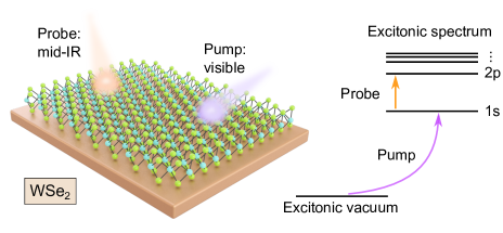
Figure 1: Pump-probe experiment for observing dark excitonic states in a transition metal dichalcogenide. The high intensity pump populates the $1$s ground state of the excitonic energy series, whereas the mid-IR low intensity probe induces transitions between the excitonic ground state ($1$s) and dark $n$p states, thus allowing to access this usually not accessible piece the of the dielectric response of the excitonic gas. This procedure is represented by the energy levels on the right part of the figure. In the left part of the figure, a sample of WSe₂ is depicted on which both the pump and the probe laser impinge.

The position of excitonic energy levels are known to depend on whether the system is confined. For example, it is well known that the Rydberg series of the two-dimensional Hydrogen atom, which in the infinite systems is given by $E_{n}=-1/[2(n-1/2)^{2}]$ with $n=1,2,3\ldots$, in atomic units, is strongly affected by confining the atom in a disk of radius $R$ Chao-Cador and Ley-Koo (2005). Recently, fabrication of transition metal dichalcogenide metamaterials with atomic precision Munkhbat et al. (2020) has opened the possibility of studying the dependence of the excitonic energy series of TMDs upon geometric confinement of different geometries. It is expected that in addition to negative energy bound states, positive ones will also appear. As we show ahead, our procedure may be applied to the study of excitons in circular boxes (which can actually be obtained, approximately, even in a hexagonal lattice).

In this paper we establish the connection between the polarizability of an exciton (a microscopic quantity) and the dielectric function, which is a macroscopic quantity characterizing many particles, when many excitons, considered non-interacting (and therefore, low density) form an excitonic gas. We show that our microscopic theory can account well for the experimental results of Poellmann et al. Poellmann et al. (2015). The paper is organized has follows: in section II we present the Fowler’s and Karplus’ method which will allow us to compute the optical polarizability without evaluating a sum over states (whose direct approach is doomed to fail). This method requires the solution of a differential equation, which is then used to compute the matrix elements that define the polarizability. Afterwards, we apply this technique to the simple case of the cylindrical potential well. The goal of this section is to benchmark the method. In section III we explore the problem of excitons in WSe₂, presenting a way of solving the Fowler’s and Karplus’ differential equation for excitonic problems, computing the polarizability and, from it, the dielectric function and conductivity of a macroscopic collection of excitons. This section ends with a comparison of our theoretical results with experimental data and a good agreement is found. In section IV we give our final remarks. An appendix showing how to solve the Wannier equation in log-grid closes the paper.

II Karplus’ and Fowler’s method

In this section we will briefly present the Karplus’ and Fowler’s Podolsky (1928); Karplus (1962); Karplus and Kolker (1963); Fowler (1984) method to compute the dynamical polarizability of different systems. After the essential features of this approach are laid out, we will explore the problem of the infinite cylindrical well. This serves two purposes: on the one hand it allows us to apply the formalism to a simple yet instructive case; and on the other, it sets the stage for the problem of two-dimensional excitons that will be treated in the subsequent section and involves the solution of the Wannier equation.

II.1 Theory

Let us begin our discussion considering the following Hamiltonian written in atomic units (a.u.; this system of units is used throughout the paper, except when stated otherwise) in the dipole approximation:

$$H =H_{0}-\mathbf{r}\cdot\mathbf{F}(t),$$ (1)

$$=-\frac{1}{2\mu}\nabla^{2}+V(\mathbf{r})-\mathbf{r}\cdot\mathbf{F}(t)$$ (2)

where $\mu$ is a mass term, $\nabla^{2}$ is the Laplacian, $V(\mathbf{r})$ is a potential energy term and $\mathbf{F}(t)$ is an external time dependent harmonic electric field:

$$\mathbf{F}(t)=F\left[e^{-i\omega t}+e^{i\omega t}\right],$$ (3)

with $\omega$ the field’s frequency and $F$ its amplitude. This general Hamiltonian can be used to describe the interaction of different systems with an external electric field. Two examples which will be treated in this work are the interaction of an electric field with a particle trapped inside a cylindrical well, and the interaction of light with excitons in 2D materials. The first will be treated ahead in the present section as an introductory problem, while the latter is the main subject of this work and will be studied in the following section.

Now, for simplicity, we consider the electric field to be applied along the $-x$ direction. With this assumption, the time dependent Schrödinger equation reads:

$$\left[H_{0}+xF(t)\right]|\psi(t)\rangle=i\frac{\partial}{\partial t}|\psi(t)\rangle,$$ (4)

where $|\psi(t)\rangle$ is the state vector describing the wave function of the system in the presence of the electric field. Following Fowler’s and Karplus’ approach, we expand the state vector in powers of $F$ as:

$$|\psi(t)\rangle =e^{-iE_{0}t}|\psi_{0}\rangle$$

$$+Fe^{-i(E_{0}-\omega)t}|\psi_{1}^{+}\rangle+Fe^{-i(E_{0}+\omega)t}|\psi_{1}^{-}\rangle+\mathcal{O}\left(F^{2}\right)$$ (5)

where $E_{0}$ and $|\psi_{0}\rangle$ are the energy and state vector, respectively, of the unperturbed system and $|\psi_{1}^{\pm}\rangle$ are the first order corrections to the state vector. Inserting this expansion in Eq. (4), and keeping only terms up to first order in $F$, we find:

$$H_{0}|\psi_{0}\rangle =E_{0}|\psi_{0}\rangle$$ (6)

$$H_{0}|\psi_{1}^{\pm}\rangle+x|\psi_{0}\rangle =\left(E_{0}\mp\omega\right)|\psi_{1}^{\pm}\rangle,$$ (7)

where the first equation is nothing more than the Schrödinger equation of the unperturbed system, and the second equation defines the first order correction $|\psi_{1}^{\pm}\rangle.$ The dynamical polarizability $\alpha(\omega)$ is defined as Karplus and Kolker (1963):

$$\alpha(\omega)=-\left(\langle\psi_{0}|x|\psi_{1}^{+}\rangle+\langle\psi_{0}|x|\psi_{1}^{-}\rangle\right),$$ (8)

such that:

$$E(\omega)=E_{0}-\frac{1}{2}\alpha(\omega)F^{2}.$$ (9)

We note that no term proportional to $F$ appears in systems with inversion symmetry (like the ones we will be considering). Note that we have departed here from the traditional Rayleigh-Schrödinger perturbation theory, which goes a step further and expands $|\psi_{1}^{\pm}\rangle$ in the basis of the unperturbed Hamiltonian.

As just said, if Rayleigh-Schrödinger time-dependent perturbation theory had been used to compute the dynamical polarizability, the final result would consist in a sum over states which, in principle, could not be exactly computed, since it would require the computation of an arbitrary large number of matrix elements whose form is unknown analytically. Also, a numerical approach to the sum over states would fail, because of the difficulty of describing the wave functions of the continuum of states. Usually, these sums are truncated and only the first terms are considered. The quality of this approximation depends on how fast the sum over states converges to a given value Henriques and Peres (2020). In comparison, the presented approach bypasses the sum over states, and requires the computation of only two matrix elements in order to obtain the dynamical polarizability, as described by Eq. (8), and, at the same time, accomplishes the summation over all states.

II.2 The infinite cylindrical well

In order to test Eq. (8), we will now explore a simple example: a particle trapped inside a 2D cylindrical potential well. For simplicity let us consider the particle to be an electron, such that $\mu=1$ (in atomic units) in Eq. (2). The potential term reads:

$$V(r)=\begin{cases}0,&r<R\\ \infty,&r>R\end{cases},$$ (10)

where $R$ is the radius of the cylindrical potential well.

Before the dynamical polarizability can be computed, the unperturbed system has to be studied. Although this is a simple system with a well established solution, we will give, for completeness, a brief description of the necessary steps to find the wave functions, and the respective energies, of the cylindrical potential well. First, the Schrödinger equation is written in cylindrical coordinates $(r,\theta)$, and a solution by separation of variables is proposed. After this is done, two equations arise. The angular equation is satisfied by a complex exponential $e^{im\theta},$ where $m$ is the angular quantum number. The radial equation yields Bessel functions of the first kind. After these two solutions are combined, the boundary condition is imposed, that is, the requirement that the wave function must vanish when $r=R$. This condition, similarly to what happens in the 1D infinite well, defines the energy spectrum. In summary, the wave functions are:

$$\psi_{nm}(r,\theta)=\frac{\mathcal{C}_{nm}}{\sqrt{2\pi}}J_{m}\left(\frac{q_{mn}r}{R}\right)e^{im\theta},$$ (11)

where $J_{m}$ is a Bessel function of the first kind, $q_{mn}$ is the $n-$th zero of $J_{m}(x)$ and $\mathcal{C}_{nm}=\sqrt{2}\left[\left|J_{m+1}(q_{mn})\right|R\right]^{-1}$ is a normalization constant. The energy spectrum reads:

$$E_{nm}=\frac{1}{2}\left(\frac{q_{mn}}{R}\right)^{2}.$$ (12)

In Table 1 we present the numerical value of a few energy levels for a system with $R=2$ a.u..

$m=0$			$m=1$
$n=1$	$n=2$	$n=3$	$n=1$	$n=2$	$n=3$
0.723	3.809	9.361	1.835	6.152	12.937

Table 1: Numerical values of the energies (in atomic units) of the infinite cylindrical potential well, for the first three states with $m=0$ and $m=1$. Transitions from the ground state $(n=1$, $m=0)$ to the states with $m=1$ require the energies: 1.112, 5.429 and 12.214.

Now that we are in possession of the unperturbed wave functions and energy spectrum, the computation of the dynamical polarizability due to the presence of a time dependent external field can be performed. In agreement with the previous section, we will consider a harmonic electric field aligned along the $x-$direction. Furthermore, we will be concerned with the polarizability of the ground state, which in this case corresponds to the state with $m=0$ and $n=1$. To compute $\alpha(\omega)$ we will have to compute the matrix elements $\langle\psi_{10}|x|\psi_{1}^{\pm}\rangle$. To do so we must first solve Eq. (7) and find $|\psi_{1}^{\pm}\rangle$. For $0<r<R$ we have:

$$\left(\frac{\mathbf{p}^{2}}{2}-E_{10}\pm\omega\right)\psi_{1}^{\pm}(\mathbf{r})=-r\cos\theta\psi_{10}(\mathbf{r}).$$ (13)

We now set $\psi_{1}^{\pm}(\mathbf{r})$ as $\left[\mathcal{P_{\pm}}(r)/\sqrt{r}\right]\cos\theta$. This transformation has two advantages, as it takes care of the angular part of the differential equation, while simultaneously eliminating any term proportional to a first derivative in $r$. With this assumption we find:

$$8r^{7/2}\psi_{10}(r)+\left[3+8r^{2}(-E_{0}\pm\omega)\right]\mathcal{P}_{\pm}(r)=4r^{2}\mathcal{P_{\pm}}^{\prime\prime}(r),$$ (14)

subject to the boundary conditions $\mathcal{P}(0)=0$ and $\mathcal{P}(R)=0$. A numerical solution to this differential equation can be easily obtained, and once this is done, computing the polarizability is a trivial step, amounting to a numerical quadrature. In Fig. 2 we plot the polarizability obtained after the differential equation was solved numerically. In order to obtain the real and imaginary parts of the polarizability, a small imaginary term was subtracted to $\omega$, that is $\omega\rightarrow\omega-i\delta$, with $\delta\ll\omega$; this parameter controls the linewidth of the resonances, and should be chosen to match experimental results. Since our goal is not to compare this simple example with experimental data we simply set $\delta=0.05$ a.u.. Inspecting the results in Fig. 2, we find that, as expected, clear resonances appear at energies corresponding to transitions from the ground state to states with $m=1$, as can be confirmed by recalling the values presented in Table 1. The first resonance, corresponding to a transition from the ground state to the state with $n=m=1$ is by far the dominant one, being orders of magnitude more intense than the second and third peaks. Although not depicted, at higher energies other peaks with even smaller oscillator strengths appear.

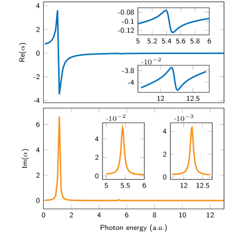
Figure 2: Plot of the real (top) and imaginary (bottom) parts of the dynamical polarizability for an infinite cylindrical well, obtained using Eq. (8), and with $\psi_{1}^{\pm}$ computed numerically. Both plots present three resonances whose positions exactly coincide with the energies associated with transitions from the state with $m=0$ and $n=1$, to the three states with $m=1$ presented in Table 1. In order to obtain the real and imaginary parts of the polarizability, a small imaginary term, $\delta=0.05$ a.u., was subtracted to $\omega$. We considered the particle to be an electron, confined to a disk of radius $R=2$ a.u..

III Application to two-dimensional excitons

In the present section we will apply the same theoretical ideas developed so far to compute the optical polarizability of excitons in 2D materials. Contrary to the case of the infinite cylindrical potential well, the existence of a Coulomb-like potential combined with an infinite geometry transforms this problem into a rather involved one. To cope with the inherent difficulties, we will consider the problem to be confined on a finite disk, and solve the Fowler-Karplus’ differential equation using a variational approach. In the end we will consider the radius of the disk to be sufficiently large so that the obtained results are numerically identical to the ones we would obtain with an infinite geometry, allowing us to compare our predictions with the experimental results of Poellmann et al Poellmann et al. (2015).

III.1 Relation between polarizability, dielectric function, and optical conductivity

Consider a gas with $N_{X}$ excitons per unit area in a two dimensional material. The concentration $N_{X}$ is controlled by the interband excitation process (fluence of the laser), the exciton recombination, and disorder. If the electric field creating the exciton gas is weak, the excitons’ concentration is small and the gas can be considered non interacting. The polarization of a 2D material due to intra-exciton transitions is defined as

$$\mathbf{P}_{{\rm ex}}^{{\rm intr.}}=N_{X}\mathbf{p}=N_{X}\alpha\mathbf{E},$$ (15)

where $\mathbf{p}$ is the dipole moment of the exciton, in units of charge times length and $\alpha$ is the polarizability, in unites of $\epsilon_{0}$ times volume, with $\epsilon_{0}$ the dielectric vacuum permittivity. The susceptibility of the exciton gas associated with intra-excitons transitions is defined has

$$\chi_{{\rm ex}}^{{\rm intra.}}=\frac{\mathbf{P}_{{\rm ex}}^{{\rm intr.}}}{\epsilon_{0}\mathbf{E}}=N_{X}\alpha/\epsilon_{0},$$ (16)

and has units of length. We note that, in addition to $\chi_{{\rm ex}}^{{\rm intra.}}$, there are other terms contributing to the total susceptibility of the excitons gas: transition from the exciton vacuum to the $n$s levels and to other even parity states, and the background susceptibility, accounting for transitions to higher-energy bands, as well as other processes contributing to the total dielectric function of a TMD Gu et al. (2019). These, however, are not the focus of this paper and have been addressed elsewhere Epstein et al. (2020). Thus, we introduce the dielectric function associated with intra-exciton transition in a diluted medium (that is, low exciton density) as,

$$\Delta\epsilon(\omega)=\chi_{{\rm ex}}^{{\rm intra.}}/d=\alpha\frac{N_{X}}{\epsilon_{0}d}\frac{1}{g_{s}g_{v}},$$ (17)

where $d$ is the effective thickness of the TMD layer and $g_{s}$ and $g_{v}$ are the spin and valley degeneracy factors.The real and imaginary parts of the dielectric function due to intra-exciton transitions follow from this equation. The relation between the dielectric function and the conductivity, $\sigma$, follows from Kaindl et al. (2009) $\Delta\epsilon=i\sigma/(\epsilon_{0}\omega)$, and we obtain

$$\sigma=-i\epsilon_{0}\omega\Delta\epsilon.$$ (18)

The computation of these two quantities, $\Delta\epsilon(\omega)$ and $\sigma$, for the $1$s$\rightarrow n$p excitonic transitions is our main goal. (It would be interesting to derive a Clausius-Mossotti Ryazanov and Tishchenko (2006), relation for two-dimensional excitons, although this is not the focus of our work.)

III.2 The variational wave function to the ground state of the exciton

In what follows we will compute the optical polarizability of the excitonic ground state ($1$s state). In order to do so, we need to first determine its wave function. Finding an analytical expression for the $1s$ exciton state is not a simple task Henriques et al. (2020a, b), and because of that we will consider the following double exponential variational ansatz to describe the ground state Pedersen (2016) (see also Quintela and Peres (2020)):

$$\psi_{0}=\mathcal{N}\left(e^{-ar}-be^{-\gamma ar}\right),$$ (19)

where $\mathcal{N}$ is a normalization constant and $a,$ $b$, and $\gamma$ are variational parameters obtained from energy minimization. This variational ansatz is considerably more accurate than if a single exponential is used. In the context of the excitonic problem, the Hamiltonian given in Eq. (2) becomes:

$$H=-\frac{1}{2\mu}\nabla^{2}+V_{{\rm RK}}(r)-\mathbf{r}\cdot\mathbf{F}(t),$$ (20)

where $\mu$ is the reduced mass of the electron-hole system, $\mathbf{F}(t)$ is the external field previously defined in Eq. (3), and $V_{{\rm RK}}(r)$ is the Rytova-Keldysh potential Rytova (1967); Keldysh (1979):

$$V_{{\rm RK}}(r)=-\frac{\pi}{2r_{0}}\left[\mathbf{H}_{0}\left(\frac{\kappa r}{r_{0}}\right)-Y_{0}\left(\frac{\kappa r}{r_{0}}\right)\right],$$ (21)

with $\kappa$ the mean dielectric constant of the media above and below the TMD, $r_{0}$ is an intrinsic parameter of the 2D material which can be related to the effective layer thickness $d$ Poellmann et al. (2015), and $\mathbf{H}_{0}$ and $Y_{0}$ are the Struve $H$-function of zero-th order and the Bessel function of the second kind of the same order, respectively. This potential is the solution of the Poisson equation for a charge embedded in a thin film. For large distances the Rytova-Keldysh potential presents a Coulomb tail, and diverges logarithmically near the origin.

Having determined a way to compute the excitonic ground state wave function and binding energy, we turn our attention to solving the Fowler’s and Karplus’ Fowler (1984); Karplus and Kolker (1963) differential equation introduced in Eq. (7). Comparing the excitonic problem with the simple example treated in the previous section, we stress two key differences. While in the case of the cylindrical well our problem had a bounded geometry, that is, the domain of our problem was necessarily restricted to $r<R$, in the present scenario we find an unbounded problem, whose domain extends up to infinity. Moreover, in the previous section no potential term appeared in our calculations, while in the present case we find the Rytova-Keldysh potential which, as previously noted, presents a Coulomb$-1/r$ tail at large distance and a $\ln(r)$ divergence at short distances. This slow decaying behavior is known to be problematic in numerical calculations. Considering these two remarks, it is clear that finding the solution to the differential equation will not be as straight forward a process as it was before.

The first step we take in order to proceed with the calculations is to confine our system on a finite disk with large radius $R$. In practice, when numerical values are introduced, we will consider $R$ to be sufficiently large in order to obtain results which are numerically identical to the ones that one would find for an unbounded problem, and thus be able to compare our results with those from Ref. Poellmann et al. (2015). This approach would also prove its usefulness if a genuinely finite system was studied. The confinement is reflected on the wave function of the ground state by the introduction of an additional multiplicative term $(r-R)$, that is:

$$\psi_{0}^{{\rm fin.}}(r)=\mathcal{N}^{{\rm fin}}\left(e^{-ar}-be^{-\gamma ar}\right)\left(r-R\right).$$ (22)

For a sufficiently large $R$ one finds:

$$\lim_{R\rightarrow\infty}\psi_{0}^{{\rm fin.}}(r)=\psi_{0}(r).$$ (23)

As before, the parameters $a,$ $b$ and $\gamma$ are determined from energy minimization. This transformation does not allow us to immediately solve the differential equation. However, it unlocks a new way of approaching the problem.

III.3 The dynamic variational method

Since we are now effectively working on a finite disk, and we saw in the previous section that Bessel functions are an appropriate complete set of functions to describe a problem in such a geometry, we propose that $\psi_{1}^{\pm}(\mathbf{r})$ can be written as:

$$\psi_{1}^{\pm}(\mathbf{r})=\cos\theta\sum_{n=1}^{N}c_{n}^{\pm}J_{1}\left(\frac{z_{1n}r}{R}\right),$$ (24)

where $J_{1}(z)$ is a Bessel function of the first kind, $z_{1n}$ is the $n-$th zero of $J_{1}(z)$, $R$ is the radius of the disk, $N$ is the number of Bessel function we choose to use, and $\left\{c_{n}^{\pm}\right\}$ are a set of coefficients yet to be determined. As proposed in Ref. Karplus and Kolker (1963); Montgomery and Rubenstein (1978); Yaris (1963, 1964) the values of $\left\{c_{n}^{\pm}\right\}$ are determined from the minimization of the following functional:

$$\mathcal{J}_{\pm} =\int d\mathbf{r}\psi_{1}^{\pm}(\mathbf{r})\left[H_{0}-E_{0}\pm\hbar\omega\right]\psi_{1}^{\pm}(\mathbf{r})$$

$$+2\int d\mathbf{r}\psi_{1}^{\pm}(\mathbf{r})r\cos\theta\psi_{0}(\mathbf{r}).$$ (25)

We now recall the following relation regarding the orthogonality of Bessel functions on a finite disk of radius $R$ Jeffrey and Zwillinger (2014):

$$\int_{0}^{R}J_{\nu}\left(\frac{\alpha_{\nu m}r}{R}\right)J_{\nu}\left(\frac{\alpha_{\nu n}r}{R}\right)rdr=\frac{R^{2}}{2}\delta_{nm}\left[J_{\nu+1}(\alpha_{\nu m})\right]^{2},$$ (26)

where $\alpha_{\nu m}$ is the $m-$th zero of $J_{\nu}(z).$ Using this relation, one easily shows that the functional can be rewritten as:

$$\mathcal{J}_{\pm} =\frac{\pi R^{2}}{2}\sum_{n=1}\left(c_{n}^{\pm}\right)^{2}\left[\frac{\hbar^{2}}{2\mu}\frac{z_{1n}^{2}}{R^{2}}-E_{0}\pm\hbar\omega\right]\left[J_{2}\left(z_{1n}\right)\right]^{2}$$

$$+\pi\sum_{n=1}\sum_{k=1}c_{n}^{\pm}c_{k}^{\pm}\mathcal{I}_{kn}+2\pi\sum_{n=1}c_{n}^{\pm}\mathcal{S}_{n},$$ (27)

where $\mathcal{S}_{n}$ and $\mathcal{I}_{kn}$ refer to the following integrals involving one and two Bessel functions, respectively:

$$\mathcal{I}_{kn} =\int J_{1}\left(\frac{z_{1k}r}{R}\right)V_{{\rm RK}}(r)J_{1}\left(\frac{z_{1n}r}{R}\right)rdr$$ (28)

$$\mathcal{S}_{n} =\int J_{1}\left(\frac{z_{1n}r}{R}\right)\psi_{0}^{{\rm fin.}}(r)r^{2}dr.$$ (29)

Remembering our goal of minimizing the functional $\mathcal{J}_{\pm}$, we must now differentiate it with respect to the different $c_{n}^{\pm}$ with $n\in\left\{1,2,...,N\right\}$. Doing so, and noting in passing that $\mathcal{I}_{kn}=\mathcal{I}_{nk}$, one finds:

$$c_{j}^{\pm}\left\{\frac{R^{2}}{2}\left[\frac{1}{2\mu}\frac{z_{1j}^{2}}{R^{2}}-E_{0}\pm\omega\right]\left[J_{2}\left(z_{1j}\right)\right]^{2}+\mathcal{I}_{jj}\right\}$$

$$+\sum_{n\neq j}^{N}c_{n}^{\pm}\mathcal{I}_{jn}=-\mathcal{S}_{j}$$ (30)

with $j\in\left\{1,2,...,N\right\}$. It is now clear that this defines a linear system of equations whose solution determines the values of the coefficients $c_{n}^{\pm}$. Moreover, we can write this concisely using matrix notation, as follows:

$$\mathbb{M}\cdot\mathbf{c}^{\pm}=-\mathbf{S},$$ (31)

where $\mathbf{c}^{\pm}$ and $\mathbf{S}$ are column vectors defined as:

$$\left[\mathbf{c}^{\pm}\right]^{{\rm T}} =\left(c_{1}^{\pm},c_{2}^{\pm},\ldots,c_{N}^{\pm}\right)$$ (32)

$$\mathbf{S}^{{\rm T}} =\left(\mathcal{S}_{1},\mathcal{S}_{2},\ldots,\mathcal{S}_{N}\right),$$ (33)

and $\mathbb{M}$ is an $N\times N$ matrix with:

$$\left(\mathbb{M}\right)_{ij}=\begin{cases}g_{i}^{\pm}(\omega)+\mathcal{I}_{ii}&i=j\\ \mathcal{I}_{ij}&i\neq j\end{cases},$$ (34)

where $g_{i}^{\pm}(\omega)=R^{2}\left[z_{1i}^{2}/(2\mu R^{2})-E_{0}\pm\omega\right]/2$. After $\mathbb{M}$ and $\mathbf{S}$ are computed using Eqs. (28) and (29), respectively, the coefficients that determine $\psi_{1}^{\pm}(\mathbf{r})$ are readily obtained:

$$\mathbf{c}^{\pm}=-\mathbb{M}^{-1}\cdot\mathbf{S},$$ (35)

and the solution of the differential equation is found. As was previously mentioned, when specific values are introduced in the problem, the radius $R$ must be chosen large enough in order to produce results which are identical to the ones of an unbounded system. As the value of $R$ increases, the value of $N$ must also increase in order to accurately describe the desired physical system. At first, this may seem problematic, since for each value of $\omega$ we would have to compute $\mathbb{M}$ (with $N^{2}$ entries) and solve the linear system associated with it. However, two aspects prevent this approach of becoming inadequately inefficient as $N$ increases: i) the matrix $\mathbb{M}$ is symmetric, reducing the number of independent entries from $N^{2}$ to $N(N+1)/2$; ii) more importantly, the most time consuming part of the calculation, computing all the relevant $\mathcal{I}_{ij}$, is independent of $\omega$, and does not need to be reevaluated every time a new energy is used.

$\mu/m_{0}$	$r_{0}$ /$a_{0}$	$\kappa$	$N_{X}$ (cm-2)	$d/a_{0}$	$R$ /$a_{0}$	$N$
0.167	$54$	3.32	1.8$\times 10^{12}$	6.04	800	35

Table 2: Parameters used to describe excitons in WSe₂. The value of $R$ was chosen in such a way that the wave functions of the first excited states are effectively zero even before $r=R$. Inspecting Figure 4, we observe that the states with $m=1$ and $n=2,3$ have wave functions which essentially vanish for $r\sim 400a_{0}$, where $a_{0}\sim 0.53$ $\AA$ is the Bohr radius. The number of Bessel functions ($N$) was chosen as the minimum number which upon addition of more functions leaves the final result unchanged. The parameters related with WSe₂were taken from Ref. Poellmann et al. (2015). The reduced mass $\mu$ is given in units of the bare electron mass $m_{0}$.

At last, to compute the dynamical polarizability we look back at Eqs. (8) and (24) and write:

$$\alpha(\omega)=-2\pi\left(\mathbf{c}^{+}(\omega)+\mathbf{c}^{-}(\omega)\right)\cdot\mathbf{S},$$ (36)

Now, to put together everything we developed so far to the test, let us consider the specific case of excitons in WSe₂. The different parameters that characterize this problem are shown in Table 2. Note that the value of the radius was chose as $R=800a_{0},$ with $a_{0}\sim 0.53$ $\AA$, the Bohr radius. The choice of this value is understood from the inspection of Fig 4, in the Appendix, where we present numerically obtained wave functions for the first excited states of WSe₂ (considering an unbounded system). There we observe that the wave functions are essentially zero for $r\sim 400a_{0}$, and thus the choice of $R=800a_{0}$ renders our problem effectively infinite. Moreover, in Table 2 we also observe that $N=35$ Bessel functions were used. This value was chosen since it corresponds to the minimum value of functions upon which addition of more functions leaves the final result invariant. Inspection of the values of $\mathbf{c}^{\pm}$ allowed us to conclude that the method converged.

III.4 Results

In Fig. 3 we depict the real part of the dielectric function and the optical conductivity, obtained from the real and imaginary parts of the the polarizability using Eqs. (17) and (18), for two different linewidths, 10 meV and 50 meV, and compare our theoretical prediction with experimental results for the latter case. The linewidths are introduced in the problem by subtracting a small imaginary part (10 or 50 meV in the present case) to the photon energy. This is also what allows us to extract both the real and imaginary parts from Eq. (17). To model the problem the values of Table 2 are used.

Let us start by looking at the cases where a broadening of 10 meV was used. Similarly to what was found for the cylindrical well, we observe two clearly visible resonances at the energies corresponding to transitions from the excitonic ground state to the first two excited states with $m=1$, that is the $2$p and $3$p states. As expected, the resonance associated with the $1s\rightarrow 2p$ transition is significantly more intense than the others. More resonances exist after the second one, but are not resolved due to the value of the broadening parameter and their smaller oscillator strength. No resonances appear above the excitonic ground state energy. If the value of $R$ was chosen smaller this may not have been the case due to the appearance of states with positive energy as a consequence of the confinement Aquino et al. (2005), however, these extra resonances would be barely visible due to the smaller oscillator strengths. The values of the binding energies of the different excitonic states were computed numerically using the Numerov-shooting method described in the Appendix.

When $\Delta=50$ meV is used (a value fixed by the phenomenological fit performed in Ref. Poellmann et al. (2015)) we observe a different scenario from the previous one. Due to the increased value of the linewidth, and the way we introduced this parameter in the calculations, the $1s\rightarrow 2p$ resonance is shifted away from its theoretical value (computed numerically using the shooting method described in the Appendix). This artifact needs to be manually corrected. Contrary to the previous case, this time only the main resonance is resolved. This is a consequence of the high value of the broadening parameter considered, as well as the proximity of the different resonances and their small oscillator strength when compared to the 1s$\rightarrow$2p transition. Moreover, for this specific scenario, we also depict the experimental results measured in Ref. Poellmann et al. (2015), where the authors found that the resonance is well described by phenomenologically modeling the $1s\rightarrow 2p$ transition with a Lorentzian oscillator. A good agreement between our theoretical prediction and the experimental result is visible. Our microscopic theory captures both the position and magnitude of the measured resonances.

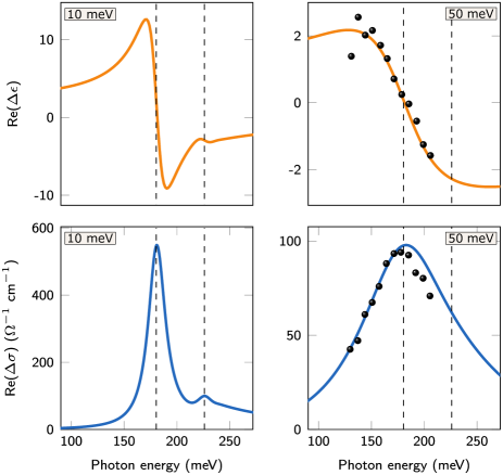
Figure 3: Real part of the dielectric function (top) and optical conductivity (bottom) for two different linewidths. 10meV (left) and 50meV (right). When a broadening of 10 meV is considered two resonances are clearly visible, appearing at energies corresponding to transitions from the ground state (1$s$) to the states $2p$ and $3p$. When a broadening of 50 meV is used, only the main resonance is resolved. For this case we also depict the experimental values measured in Ref. Poellmann et al. (2015) (large black dots). The agreement between our theoretical prediction and the experimental points is remarkable. The parameters of Table 2 were used. The energies corresponding to the transitions above mentioned are given in Table 3. The vertical dashed lines represent the energy difference $E=E_{n{\rm p}}-E_{1{\rm s}}$ as determined from the solution of the Wannier equation. As shown in the experiments Poellmann et al. (2015), the there is a relation between the level broadening and the exciton’s concentration. Therefore, the panels on the left-hand side of this figure do not represent a realistic experimental situation but rather show the role that reducing the broadening has in revealing higher energy dark states.

IV Conclusions

In this paper we have used Fowler’s and Karplus’ methods to access the polarizability of 2D excitons when transitions from bright ($n$s) states to dark ($n$p) states take place.

For benchmarking this method we first applied it to a single particle in a two dimensional disk of radius $R$ with vanishing Dirichlet boundary conditions (we note that the optical properties of condensed matter systems are sensitive to the boundary conditions Montgomery and Pupyshev (2016)). We showed that the peaks in the polarizability are in good agreement with the energy difference between the ground state and the excited states of the particle in the disk.

Afterwards, we applied Fowler’s and Karplus’ method to the central problem of our work, that of finding the dielectric function of the exciton gas. To do so, we looked for the transitions from bright ($n$s) to dark ($n$p) states, which can be accessed in pump-probe experiments. We chose the transition metal dichalcogenide WSe₂ as our test subject, since measurements of the dielectric function due to the exciton gas have been made recently Poellmann et al. (2015). We found a good agreement between the results obtained from our microscopic theory and the experimental data. Indeed the Fowler-Karplus approach allows us to access the excitonic response of the system without much work, only requiring the knowledge of the ground state of the excitonic problem. This is a major advantage over the overwhelming fully computational calculations based on ab-initio methods. For making our work mostly analytical, we use an analytical variational wave function to describe the ground state of the exciton problem. The numerical part of the calculation consists on computing and solving a well behaved linear system of equations. The role of disorder on the visibility of $1$s$\rightarrow n$p transitions was also discussed. We showed that for small disorder, $\Delta=10$ meV, several transitions to different $n$p states are visible in the polarizability spectrum, whereas for large disorder, $\Delta=50$ meV, the first transition $1$s$\rightarrow 2$p is rather broad, as seen in the experiments, and higher order transition are masked by the linewidth of the peak.

Finally, we speculate that a similar experiment made on WSe₂ encapsulated in boron-nitride will allow the revealing of the transition to higher $n$p rather than just the $1$s$\rightarrow 2$p transition. The nonlinear response of the exciton gas Mossman et al. (2016); Kocherzhenko et al. (2019) will be the subject of a future work.

Appendix A Numerov shooting method and the Schrödinger equation in a log-grid

In this appendix we give a description of the method used to compute the binding energies of excitons in WSe₂. To compute these energies one needs to solve the Wannier equation (in atomic units):

$$-\frac{1}{2\mu}\nabla^{2}\psi(\mathbf{r})+V_{{\rm RK}}(r)\psi(\mathbf{r})=E\psi(\mathbf{r}),$$ (37)

where, as in the main text, $\mu$ is the reduced mass of the electron-hole system, $V_{{\rm RK}}$ is the Rytova-Keldysh potential defined in Eq. (21), $\psi(\mathbf{r})$ is the exciton wave function, and $E$ its binding energies.

In order to solve this equation, we propose the usual solution by separation of variables, such that $\psi(\mathbf{r})=R(r)\Theta(\theta)$. The angular contribution trivially yields:

$$\Theta(\theta)=\frac{e^{im\theta}}{\sqrt{2\pi}},$$ (38)

where $m=0,\pm 1,\pm 2,...$ is the angular quantum number, and the $\sqrt{2\pi}$ is a normalization factor. Considering the definition $u(r)=R(r)\sqrt{r}$, the radial equation becomes:

$$-\frac{1}{2\mu}\frac{d^{2}u}{dr^{2}}+\left[\frac{m^{2}}{2\mu r^{2}}-\frac{1}{8\mu r^{2}}+V_{{\rm RK}}(r)\right]u(r)=Eu(r).$$ (39)

Now, we found it useful to introduce the following change of variable:

$$x=\ln r,$$ (40)

which effectively transforms our problem from a linear to a logarithmic one. This transformation proved to be useful in the stabilization of the numerical calculations due to the divergent behavior of the Rytova-Keldysh potential at the origin. Moreover, we introduce an auxiliary function, $f,$ defined as:

$$u(x)=f(x)e^{x/2}.$$ (41)

Doing so, the radial differential equation is transformed into:

$$-\frac{1}{2\mu}f^{\prime\prime}(x)+\left[\frac{m^{2}}{2\mu}+e^{2x}V_{{\rm RK}}(e^{x})\right]f(x)=e^{2x}Ef(x),$$ (42)

with boundary conditions $f(\pm\infty)=0$. This is the equation that, when solved, defines the binding energies for the excitons in WSe₂. This equation performs outstandingly for the usually problematic $m=0$ energy levels, where the centrifugal barrier is absent.

To solve this equation we use the shooting method coupled to a Numerov algorithm Izaac and Wang (2018); Berghe et al. (1989); Johnson (1978, 1977); Pillai et al. (2012). Given an initial energy guess, we integrate Eq. (39) from left to right, and from right to left, and match the logarithmic derivatives of two solutions somewhere sufficiently away from the edges. The matched wave function will only represent a true bound state, with a correct binding energy, when both the wave function itself as well as its derivative are continuous across the whole domain. If this condition is not satisfied, a new energy guess must be used and the process repeated. The choice of the starting points of integration is of crucial importance to obtain faithful results. The staring point on the left should be chosen as negative as possible in order to accurately capture the behavior near $r=0$ (or $x\rightarrow-\infty$). In practice, values such as $x_{{\rm min}}=-10$ already produce excellent results. The starting point on the right should be chosen such that the wave function has effectively reached zero significantly before $x_{{\rm max}}.$ Using semi-analytical methods, such as the one studied in Ref. Henriques et al. (2020a), allows one to compute a first guess of the wave function, and thus determine what value of $x_{{\rm max}}$ should be chosen in the application of the shooting-Numerov method. The method of Ref. Henriques et al. (2020a) is also a good starting point for the initial guesses of the binding energies. In Ref. Izaac and Wang (2018) an efficient algorithm to find the binding energies of Coulomb-like problems is described. The method is numerically stable and fast.

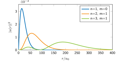
Figure 4: Probability radial density of the the ground state ($n=1$ and $m=0$) and the first excited states with $m=1$, of excitons in WSe₂, obtained using the shooting method. The parameters of Table 2 were used. The radius is given in units of Bohr’s radius $a_{0}\approx 0.53$ $\AA$.

Using the previously described method, and the parameters presented in Table 2 of the main text, we were able to compute the wave functions of the ground state, and the first two excited states with $m=1$, of excitons in WSe₂ depicted in Figure 4. As expected, these wave functions resemble those one would obtain with the Coulomb potential. However, since the Rytova-Keldysh potential originates states with smaller binding energies than the Coulomb potential, these wave functions are more spread out in space. Although only three wave functions are presented, this method also allows the computation of higher excited states.

$m=0$	$m=1$
$n=1$	$n=2$	$n=3$	$n=4$	$n=5$
$-255$	$-75$	$-29$	$-15$	$-9$

Table 3: Binding energies (in meV) of a few excitonic states in WSe₂, obtained with the shooting method. The parameters of Table 2 were used. The energy difference $\Delta E=-75+255=180$ meV coincides very well with the value observed in the experiment at moderate densities of the exciton gas.

The binding energies of the ground state, as well as the first states with $m=1$, are presented in Table 3. These energies, and in particular those corresponding to the transitions $1s\rightarrow 2p$ and $1s\rightarrow 3p$, are in agreement with Figure 3 of the main text.

References

- Lv et al. (2015) R. Lv, J. A. Robinson, R. E. Schaak, D. Sun, Y. Sun, T. E. Mallouk, and M. Terrones, Accounts of Chemical Research 48, 56 (2015).
- Ma et al. (2020) Q. Ma, G. Ren, K. Xu, and J. Z. Ou, Advanced Optical Materials , 2001313 (2020).
- Mueller and Malic (2018) T. Mueller and E. Malic, npj 2D Materials and Applications 2, 1 (2018).
- Wang et al. (2018) G. Wang, A. Chernikov, M. M. Glazov, T. F. Heinz, X. Marie, T. Amand, and B. Urbaszek, Reviews of Modern Physics 90, 021001 (2018).
- Mak et al. (2018) K. F. Mak, D. Xiao, and J. Shan, Nature Photonics 12, 451 (2018).
- Schneider et al. (2018) C. Schneider, M. M. Glazov, T. Korn, S. Höfling, and B. Urbaszek, Nature Communications 9, 2695 (2018).
- Hsu et al. (2019) W.-T. Hsu, J. Quan, C.-Y. Wang, L.-S. Lu, M. Campbell, W.-H. Chang, L.-J. Li, X. Li, and C.-K. Shih, 2D Materials 6, 025028 (2019).
- Chaves et al. (2017) A. J. Chaves, R. M. Ribeiro, T. Frederico, and N. M. R. Peres, 2D Materials 4, 025086 (2017).
- Zhang et al. (2017) X.-X. Zhang, T. Cao, Z. Lu, Y.-C. Lin, F. Zhang, Y. Wang, Z. Li, J. C. Hone, J. A. Robinson, D. Smirnov, S. G. Louie, and T. F. Heinz, Nature Nanotechnology 12, 883 (2017).
- Yong et al. (2019) C.-K. Yong, M. I. B. Utama, C. S. Ong, T. Cao, E. C. Regan, J. Horng, Y. Shen, H. Cai, K. Watanabe, T. Taniguchi, S. Tongay, H. Deng, A. Zettl, S. G. Louie, and F. Wang, Nature Materials 18, 1065 (2019).
- Steinleitner et al. (2017) P. Steinleitner, P. Merkl, P. Nagler, J. Mornhinweg, C. Schüller, T. Korn, A. Chernikov, and R. Huber, Nano Letters 17, 1455 (2017).
- Koperski et al. (2017) M. Koperski, M. R. Molas, A. Arora, K. Nogajewski, A. O. Slobodeniuk, C. Faugeras, and M. Potemski, Nanophotonics 6, 1289 (01 Nov. 2017).
- Miyajima et al. (2016) K. Miyajima, K. Sakaniwa, and M. Sugawara, Physical Review B 94, 195209 (2016), publisher: American Physical Society.
- Berghäuser et al. (2016) G. Berghäuser, A. Knorr, and E. Malic, 2D Materials 4, 015029 (2016).
- Berghäuser et al. (2018) G. Berghäuser, P. Steinleitner, P. Merkl, R. Huber, A. Knorr, and E. Malic, Physical Review B 98, 020301 (2018).
- Merkl et al. (2019) P. Merkl, F. Mooshammer, P. Steinleitner, A. Girnghuber, K.-Q. Lin, P. Nagler, J. Holler, C. Schüller, J. M. Lupton, T. Korn, S. Ovesen, S. Brem, E. Malic, and R. Huber, Nature Materials 18, 691 (2019).
- Tian et al. (2020) T. Tian, D. Scullion, D. Hughes, L. H. Li, C.-J. Shih, J. Coleman, M. Chhowalla, and E. J. G. Santos, Nano Letters 20, 841 (2020).
- Wang et al. (2006) F. Wang, J. Shan, M. A. Islam, I. P. Herman, M. Bonn, and T. F. Heinz, Nature Materials 5, 861 (2006).
- Poellmann et al. (2015) C. Poellmann, P. Steinleitner, U. Leierseder, P. Nagler, G. Plechinger, M. Porer, R. Bratschitsch, C. Schüller, T. Korn, and R. Huber, Nature Materials 14, 889 (2015).
- Cha et al. (2016) S. Cha, J. H. Sung, S. Sim, J. Park, H. Heo, M.-H. Jo, and H. Choi, Nature Communications 7, 10768 (2016).
- Sie et al. (2015) E. J. Sie, J. W. McIver, Y.-H. Lee, L. Fu, J. Kong, and N. Gedik, Nature Materials 14, 290 (2015).
- Fröhlich et al. (1985) D. Fröhlich, A. Nöthe, and K. Reimann, Physical Review Letters 55, 1335 (1985).
- Zhang et al. (2015) X.-X. Zhang, Y. You, S. Y. F. Zhao, and T. F. Heinz, Physical Review Letters 115, 257403 (2015).
- Chao-Cador and Ley-Koo (2005) L. Chao-Cador and E. Ley-Koo, International Journal of Quantum Chemistry 103, 369 (2005).
- Munkhbat et al. (2020) B. Munkhbat, A. B. Yankovich, D. G. Baranov, R. Verre, E. Olsson, and T. O. Shegai, Nature Communications 11, 4604 (2020).
- Podolsky (1928) B. Podolsky, Proceedings of the National Academy of Sciences 14, 253 (1928).
- Karplus (1962) M. Karplus, The Journal of Chemical Physics 37, 2723 (1962).
- Karplus and Kolker (1963) M. Karplus and H. J. Kolker, The Journal of Chemical Physics 39, 1493 (1963).
- Fowler (1984) P. W. Fowler, Molecular Physics 53, 865 (1984).
- Henriques and Peres (2020) J. C. G. Henriques and N. M. R. Peres, Phys. Rev. B 101, 035406 (2020).
- Gu et al. (2019) H. Gu, B. Song, M. Fang, Y. Hong, X. Chen, H. Jiang, W. Ren, and S. Liu, Nanoscale 11, 22762 (2019).
- Epstein et al. (2020) I. Epstein, B. Terres, A. J. Chaves, V.-V. Pusapati, D. A. Rhodes, B. Frank, V. Zimmermann, Y. Qin, K. Watanabe, T. Taniguchi, H. Giessen, S. Tongay, J. C. Hone, N. M. R. Peres, and F. H. L. Koppens, Nano Letters 20, 3545 (2020).
- Kaindl et al. (2009) R. A. Kaindl, D. Hägele, M. A. Carnahan, and D. S. Chemla, Phys. Rev. B 79, 045320 (2009).
- Ryazanov and Tishchenko (2006) M. I. Ryazanov and A. A. Tishchenko, Journal of Experimental and Theoretical Physics 103, 539 (2006).
- Henriques et al. (2020a) J. C. G. Henriques, G. B. Ventura, C. D. M. Fernandes, and N. M. R. Peres, Journal of Physics: Condensed Matter 32 (2020a), 10.1088/1361-648X/ab47b3.
- Henriques et al. (2020b) J. C. G. Henriques, G. Catarina, A. T. Costa, J. Fernández-Rossier, and N. M. R. Peres, Phys. Rev. B 101, 045408 (2020b).
- Pedersen (2016) T. G. Pedersen, Physical Review B 94, 125424 (2016).
- Quintela and Peres (2020) M. F. C. M. Quintela and N. M. R. Peres, The European Physical Journal B 93, 222 (2020).
- Rytova (1967) S. Rytova, Moscow University Physics Bulletin 22 (1967).
- Keldysh (1979) L. Keldysh, Sov. J. Exp. and Theor. Phys. Lett. 29, 658 (1979).
- Montgomery and Rubenstein (1978) H. E. Montgomery and T. G. Rubenstein, Chemical Physics Letters 58, 295 (1978).
- Yaris (1963) R. Yaris, The Journal of Chemical Physics 39, 2474 (1963).
- Yaris (1964) R. Yaris, The Journal of Chemical Physics 40, 667 (1964).
- Jeffrey and Zwillinger (2014) A. Jeffrey and D. Zwillinger, eds., Table of Integrals, Series, and Products, 8th ed. (Academic Press, Amsterdam ; Boston, 2014).
- Aquino et al. (2005) N. Aquino, G. Campoy, and A. Flores-Riveros, International Journal of Quantum Chemistry 103, 267 (2005).
- Montgomery and Pupyshev (2016) H. E. Montgomery and V. I. Pupyshev, Physica Scripta 92, 015401 (2016).
- Mossman et al. (2016) S. Mossman, R. Lytel, and M. G. Kuzyk, JOSA B 33, E31 (2016).
- Kocherzhenko et al. (2019) A. A. Kocherzhenko, S. V. Shedge, X. Sosa Vazquez, J. Maat, J. Wilmer, A. F. Tillack, L. E. Johnson, and C. M. Isborn, The Journal of Physical Chemistry C 123, 13818 (2019).
- Izaac and Wang (2018) J. Izaac and J. Wang, Computational Quantum Mechanics, Undergraduate Lecture Notes in Physics (Springer International Publishing, 2018).
- Berghe et al. (1989) G. V. Berghe, V. Fack, and H. E. D. Meyer, Journal of Computational and Applied Mathematics 28, 391 (1989).
- Johnson (1978) B. R. Johnson, The Journal of Chemical Physics 69, 4678 (1978).
- Johnson (1977) B. R. Johnson, The Journal of Chemical Physics 67, 4086 (1977).
- Pillai et al. (2012) M. Pillai, J. Goglio, and T. G. Walker, American Journal of Physics 80, 1017 (2012).