A series of spectral gaps for the almost Mathieu operator with a small coupling constant

Abstract.

For the almost Mathieu operator with a small coupling constant $\lambda$, for a series of spectral gaps, we describe the asymptotic locations of the gaps and get lower bounds for their lengths. The number of the gaps we consider can be of the order of $\ln 1/\lambda$, and the length of the $k$-th gap is roughly of the order of $\lambda^{k}$.

1. Introduction

We consider the almost Mathieu operator acting in $l^{2}({\mathbb{Z}})$ by the formula

(1.1) $$(H_{\theta}f)_{k}=f_{k+1}+f_{k-1}+2\lambda\cos(2\pi(\theta+hk))f_{k},\quad k\in{\mathbb{Z}},$$

where $\lambda>0$,  $0\leq\theta<1$, and $0<h<1$ are parameters. The parameter $\lambda$ is called a coupling constant. The operator (1.1) arises when studying an electron in a crystal submitted to a constant magnetic field when the field is weak, when it is strong, in semiclassical regime etc, see, e.g., [15] and references therein. This operator attracts attention of mathematicians as well as physicists thanks to its rich and unusual properties. One of the most difficult and interesting problems is the problem of describing the geometry of the spectrum of $H_{\theta}$. During three decades, efforts of many mathematicians have been aimed at proving that for irrational $h$ the spectrum is a Cantor set. Among them are A. Avila, J. Bellissard, B. Helffer, S.Zhitomirskaya, R. Krikorian, Y. Last, J. Puig, B. Simon, J. Sjöstrand and many others, see [1], where the proof was completed. We mention also [17, 18, 19] that are ones of the latest papers on the geometry of the spectrum.

Among the papers of physicists explaining the cantorian structure of the spectrum, we single out the paper [23] containing heuristic analysis clear for mathematicians. In the semiclassical approximation, the author has successively described sequences of shorter and shorter spectral gaps, i.e., obtained a constructive description of the spectrum as a Cantor set. According to [23], the spectrum located on certain intervals of the real line, being “put under a microscope”, looks like the spectrum of the almost Mathieu operator with new parameters. That is why the approach described by Wilkinson is called a renormalization method. Using methods of the pseudodifferential operator theory, B. Helffer and J. Sjöstrand have developed a rigorous asymptotic renormalization method, and turned the heuristic results into mathematical theorems.
Let us note that the asymptotic renormalization methods are used when the parameter $h$ can be represented as a continued fraction with sufficiently large elements.
Later, V. Buslaev and A. Fedotov suggested the monodromization method, one more renormalization approach that arose when trying to use the Bloch-Floquet theory ideas to study the geometry of the spectrum of difference operators in $L^{2}(\mathbb{R})$. The method was further developed by A.Fedotov and F.Klopp when studying adiabatic quasiperiodic operators. More details can be found in review [10]. The monodromization method can be used for one-dimensional two-frequency difference and differential quasiperiodic operators independently of any assumptions on the continued fraction. If such an equation contains an asymptotic parameter, one can effectively describe the asymptotic geometry of the spectrum. In [10] we described how to apply the monodromization method to get a constructive asymptotic description of the spectrum as a Cantor set in the case studied by B. Helffer and J. Sjöstrand. The present paper is the first step to a similar constructive asymptotic description in the case of a small coupling constant. Here, we make only the first renormalization. This allows to describe asymptotically a series of the longest spectral gaps. We get asymptotic formulas for the gap centers and lower bounds for the gap lengths. Note that, the number of the gaps we describe can be of the order of $\ln(1/\lambda)$, and the length of the $k$-th gap is roughly of the order of $\lambda^{k}$. So, it can be difficult to get such results by means of standard perturbation methods.
The results we prove in this paper were partially announced in the short note [13].

Below $C$ denotes positive constants independent of any parameters, variables and indices, $H$ denotes expressions of the form $Ce^{C/h}$. When writing $a=O(b)$, we mean that $|a|\leq C|b|$, and when writing $a=O_{H}(b)$, we mean that $|a|\leq e^{C/h}|b|$.
Furthermore, for $z\in\mathbb{C}$, we often use the notations $x={\rm Re}\,z$ and $y={\rm Im}\,z$.
For $v_{1},\,v_{2}\in\mathbb{C}^{2}$, we denote by $V=(v_{1}\;v_{2})$ the matrix with the columns $v_{12}$ and $v_{2}$.

2. Main results

It is well known, see, for example, [16], that for the irrational $h$, as a set, the spectrum of the almost Mathieu operator is independent of the parameter $\theta$ and coincides with the spectrum of the Harper operator acting in $L^{2}({\mathbb{R}})$ by the formula $H\psi(x)=\psi(x+h)+\psi(x-h)+2\lambda\cos(2\pi x)\psi(x)$. It is a difference Schrödinger operator with a $1$-periodic potential. Below we discuss only it.
As for the one-dimensional periodic differential operators, for the operator $H$ one can define a monodromy matrix. Here, we describe asymptotics of a monodromy matrix and spectral results obtained by means of these asymptotics.

2.1. Monodromy matrix

2.1.1.

Let us consider the Harper equation

(2.1) $$\psi(x+h)+\psi(x-h)+2\lambda\cos(2\pi x)\psi(x)=E\psi(x),\quad x\in{\mathbb{R}},$$

where $E\in{\mathbb{C}}$ is a spectral parameter. Its solution space is invariant with respect to translation by one. Let us fix a basis in the solution space. The corresponding monodromy matrix represents the restriction of the translation operator to the solution space. Equation (2.1) is a second order difference equation on $\mathbb{R}$, and its solution space is a two-dimensional modul over the ring of $h$-periodic functions, see, e.g. [6]. Thus, the monodromy matrix is a $2\times 2$ matrix $h$-periodic in $x$. When defining a monodromy matrix, it is convenient to make a linear change of variables, for it to be $1$-periodic. The formal definitions can be found in sections 3.1.1 and 3.1.3.
The following two theorems describe the functional structure of one of the monodromy matrices.

Theorem 2.1.

In the solution space of (2.1), there exists a basis such that the corresponding monodromy matrix is of the form

(2.2) $${\mathcal{M}}(x)=\left(\begin{array}[]{cc}a-2\lambda_{1}\cos(2\pi x)&s+t\,e^{\textstyle-2\pi ix}\\ {}\hfil\\ -s-t\,e^{\textstyle 2\pi ix}&st/\lambda_{1}\end{array}\right),\ \ a=\lambda_{1}\frac{1-s^{2}-t^{2}}{st},\ \ \lambda_{1}=\lambda^{\frac{1}{h}},$$

where the coefficients $s$ and $t$ are independent of $x$ and meromorphic in $E$.

This theorem is a part of Theorem 7.3 from  [6]. The basis solutions are minimal entire solutions, i.e., solutions that are entire functions of $z=x+iy$ growing the most slowly as $|y|\to\infty$. These minimal solutions are meromorphic in $E$.

Remark 2.1.

It follows from the proof of this theorem that if, for given $h=h_{0}\in(0,1)$, $\lambda=\lambda_{0}\in(0,\infty)$, and $E=E_{0}\in\mathbb{C}$, the coefficients $s$ and $t$ are finite, then they are continuous in $(h,\lambda,E)$ in a neighborhood of $(h_{0},\lambda_{0},E_{0})$.

In Section 6, we check

Theorem 2.2.

If for an $E\in{\mathbb{R}}$ the coefficient $t$ is finite, then, for this $E$,

(2.3) $$t\in i{\mathbb{R}},\quad|s|=\lambda_{1}\sqrt{\frac{1+|t|^{2}}{\lambda_{1}^{2}+|t|^{2}}},$$

and the zeroth Fourier coefficient of the trace of the monodromy matrix equals

(2.4) $$L=\frac{2i}{t}\sqrt{(1+|t|^{2})(\lambda_{1}^{2}+|t|^{2})}\cos({\rm arg}\,(is)).$$

Relations  (2.3) and (2.4) reflect the self-adjointness of the Harper operator.

2.1.2.

Pick $a\in(0,\pi)$. The asymptotics of the coefficients $s$ and $t$ as $\lambda\to 0$ are described in terms of a meromorphic function $\sigma_{a}$ satisfying the equation

(2.5) $$\sigma_{a}(z+a)=(1+e^{-iz})\sigma_{a}(z-a),\quad z\in{\mathbb{C}}.$$

Let $S=\{z\in{\mathbb{C}}\,:\,|{\rm Re}\,z|<\pi+a\}$. The function $\sigma_{a}$ is uniquely characterized by the following properties. In the strip $S$, it is analytic, does not vanish, tends to one as $y\to-\infty$ and has the minimal possible growth as $y\to+\infty$. This function and functions related to it arose in different areas of mathematical physics, see, e.g., [6, 2, 3, 8, 12, 20, 22]. We discuss $\sigma_{a}$ in section 8. Let

(2.6) $$F_{0}(p)=\sigma_{\pi h}(4\pi p-\pi+\pi h)\,\overline{\sigma_{\pi h}(4\pi\overline{p}-\pi+\pi h)}.$$

To describe the asymptotics of $t$ and $s$, we also use the parameter $p$ related to $E$ by the equation

(2.7) $$E=2\cos(2\pi p),$$

and the notation $\xi=\frac{1}{2\pi}\ln\lambda$.

Theorem 2.3.

Fix $\beta\in(0,1/2)$. There exists $c>0$ such that if $\lambda<e^{-c/h}$, then, for $p$ satisfying the inequalities $|{\rm Im}\,p|\leq h$ and $h/4<{\rm Re}\,p<1/2-h/4$, one has

(2.8) $$t=\frac{ie^{\frac{4\pi(1/2-p)\xi}{h}}F_{0}(p)}{2\sin(2\pi p)}\,(1+O_{H}(\lambda^{\beta})),\quad s=\frac{-2i\,e^{\frac{4\pi p\xi}{h}+\frac{2\pi ip}{h}}\,\sin(2\pi p)}{F_{0}(p)}\,(1+O_{H}(\lambda^{\beta})).$$

Note that, in the case of this theorem, one has $st/\lambda_{1}=e^{\frac{2\pi ip}{h}}(1+O_{H}(\lambda^{\beta}))$.
The asymptotics of $s$ and $t$ near the points $p=0$ and $p=1/2$ are more complicated. They are described by Theorem 7.1.

To get the asymptotics of $s$ and $t$, we obtain asymptotics of minimal entire solutions to equation (2.1) as $\lambda\to 0$. For this, first, we construct entire solutions to the auxiliary equations $\psi(x+h)+\psi(x-h)+\lambda e^{\mp 2\pi ix}\psi(x)=E\psi(x)$. Next, in the half-planes ${\mathbb{C}}_{\pm}$ respectively, for sufficiently small $\lambda$, we construct analytic solutions to the Harper equation that are close to the solutions to the auxiliary equations. Finally, with the help of a Riemann-Hilbert problem, we make of these analytic solutions the minimal entire solutions.

Our asymptotic method works if $\lambda<e^{-c/h}$. If $h$ is so small that $\lambda>>e^{-c/h}$, then the asymptotics of the solutions to the Harper equation can be obtained by semiclassical methods, see, e.g., [4].

2.2. Spectral gaps

The first renormalization of the monodromization method consists in replacing equation   (2.1) with the first monodromy equation

(2.9) $$\Psi_{1}(x+h_{1})=M_{1}(x)\Psi_{1}(x),\quad x\in{\mathbb{C}},\qquad h_{1}=\{1/h\},$$

where $M_{1}$ is a monodromy matrix, and $\{\cdot\}$ is the fractional part. Equations (2.1) and (2.9) simultaneously have pairs of linearly independent solutions such that one solution of a pair decays exponentially as $x\to+\infty$, and the other decays as $x\to-\infty$, see Corollary 3.1. This allows to find gaps in the spectrum of the Harper equation by studying solutions to the monodromy equation. In section 3.2 we prove

Theorem 2.4.

Let $I\subset{\mathbb{R}}$ be an open interval. There exists such a constant $C$ independent of $h$ and $E$ that if

(2.10) $$(L/2)^{2}\geq(1+C\lambda_{1})(1+|t|^{2}),\quad\lambda_{1}\leq|t|\leq 1,\qquad\forall E\in I,$$

then $I$ is in a gap of the Harper operator.

It is useful to compare this theorem with a well-known theorem from the theory of the one-dimensional periodic differential Schrödinger operators. The latter says that the spectrum of a periodic operator is located on the intervals where the absolute value of the trace of a monodromy matrix is less than or equal to two.

Using Theorem 2.4, formula (2.4) and the asymptotics $s$ and $t$ described in Theorem 2.3, one can describe a sequence of the longest gaps in the spectrum of the Harper operator. As its spectrum is symmetric with respect to zero, and as the spectra for the frequencies $h$ and $1-h$ coincide, we consider only the spectrum located on ${\mathbb{R}}_{+}$ in the case where $0<h<1/2$. Let $[\cdot]$ be the integer part. One has

Theorem 2.5.

Let $h\in(0,1/2)$ and $\beta\in(0,1/2)$. Let $\lambda\leq e^{-c/h}$ with a sufficiently large $c$. There exist points $E_{k}>0$,  $1\leq k\leq K$,   $K=[1/2h]$, such that

$$E_{k}=2\cos(\pi hk+O_{H}(\lambda^{p})),$$

and, if $1\leq k\leq K-1$ or if $k=K$ and $[1/h]$ is odd, then the point $E_{k}$ is located inside a gap $g_{k}$. The length of $g_{k}$ satisfies the estimate

(2.11) $$|g_{k}|\geq 4\left(\frac{\lambda}{4}\right)^{k}\;\frac{(1+O_{H}(\lambda^{\beta}))}{\sin^{2}(\pi h)\sin^{2}(2\pi h)\dots\sin^{2}(\pi h(k-1))}$$

where for $k=1$ the product of the sines has to be replaced with one.
If $[1/h]$ be even, and $\lambda^{h_{1}}\leq e^{-c/h}$, then the point $E_{K}$ also is located in a gap $g_{K}$, and the length of $g_{K}$ satisfies (2.11) with $\beta$ replaced with $p=\min\{h_{1},\beta\}$.

In the next paper, we will prove that the expression in the right hand side of (2.11) is the leading term of the asymptotics of the length of the $k$th gap.
Theorem 2.5 agree well with the results of computer calculations described in [15].
The $K$th gap in the case where where $[1/h]$ is even is the most difficult to describe. For small $hh_{1}$, it is located near zero that is a very special point. For $h\not\in\mathbb{Q}$, the complexity of the spectrum near zero is well-known. One can find a series of new results in [17].

The right hand side in (2.11) equals $\lambda^{k}e^{O(1/h)}$, see Corollary 3.4. Therefore, if $\lambda$ is small, and $h$ is of the order of $\frac{1}{|\ln\lambda|}$, then $|g_{K}|$, the length of the gap closest to zero, is of the order of $\lambda^{|\ln\lambda|+O(1)}$. So, it can be rather difficult to compute $|g_{K}|$ using standard perturbation methods.

According to [18], for the almost Mathieu equation with $\lambda<1$ and Diophantine frequencies, as the gap number, say, $k$ tends to infinity, the gap lengths are bounded from above and below by expressions of the form $C(\lambda,h,\epsilon)\lambda^{(1\pm\epsilon)k}$, where $\epsilon$ is a fixed positive number. And as we mentioned, in our case, one has $|g_{k}|\geq\lambda^{k}e^{O(1/h)}$.

It is interesting to compare our results with the results obtained in the case of small $h$ and $\lambda=1$, see [10]. In this case, there is a statement similar to Theorem 2.4. However, the asymptotics of the coefficients $t$ and $s$ turn out to be quite different, and, on the most of the interval $[-4,4]$ containing the spectrum, $L(E)$ oscillates with an amplitude that is exponentially large with respect to $h$ , whereas in our case, for most $E\in(0,2)$, one has $L\approx 2\cos(p/h)$. Thus, in the case of small $h$, the spectrum is located on a series of exponentially small intervals, and in the case of small $\lambda$, we observe small gaps in the spectrum.

2.3. Other gaps

Since the matrix $M_{1}$ is $1$-periodic, for equation (2.9), we can also define a monodromy matrix $M_{2}$ and consider the second monodromy equation that can be obtained from the first one by replacing $M_{1}$ with $M_{2}$ and $h_{1}$ with $h_{2}=\{1/h_{1}\}$. Continuing, we can construct an infinite sequence of difference equations. In the next paper, studying consequently the equations of this sequence, we will describe consequently series of shorter and shorter gaps. We also obtain upper bounds for the gaps lengths.

Note that, to prove Theorem 2.5, we use only the asymptotics of the coefficients $s$ and $t$ from Theorem 2.3, i.e., their asymptotics for $E$ being bounded away from $2$. However, the asymptotics of $s$ and $t$ for $E$ close to $2$ are crucial to study the geometry of the spectrum near its edge. All we need to get these asymptotics is prepared when proving Theorem 2.3, and they are obtained almost like the ones described in this theorem. So, omitting elementary details, we get them in section 7.4.

2.4. The plan of the paper

In section 3, we give the definition of a monodromy matrix, and prove Theorems 2.4 and 2.5. For this we use Theorems 2.1–2.3. The most of the remaining part of the paper is devoted to the proof of Theorem 2.3. In section 4, we construct and analyze analytic solutions to the model equation (4.1). In section 5, we show that, in the upper half-plane, there are analytic solutions to the Harper equation that are close to the solutions to the model equation. Recall that the monodromy matrix described in Theorem 2.1 corresponds to a basis of two minimal entire solutions to the Harper equation. In section 6, we recall the definition of minimal entire solutions and prove Theorem 2.2. In section 7, for sufficiently small $\lambda$, using the analytic solutions to the Harper equation constructed in section 5, we construct and study the minimal entire solutions, and prove Theorem 2.3. Section 7.4 is devoted to the asymptotics of $s$ and $t$ for $p$ close to zero (i.e., for $E$ close to 2). In Section 8, we describe the properties of $\sigma_{a}$ that are used in this paper.

3. Monodromy matrices, monodromy equation and spectral results

Here we remind the definition of a monodromy matrix, describe relations between solutions to a difference equation with periodic coefficients and solutions to a corresponding monodromy equation, and prove Theorems 2.4 and 2.5.

3.1. Monodromy matrices and monodromy equation

3.1.1. Definition and elementary properties of a monodromy matrix

Here, following [10] we discuss the difference equations of the form

(3.1) $$\Psi(x+h)=M(x)\Psi(x),$$

where $x$ is a real variable, $M:{\mathbb{R}}\to SL(2,{\mathbb{C}})$ is a given 1-periodic function, and $h\in(0,1)$ is a fixed number.
Obviously, for any solution $\Psi$ to (3.1), we have $\det\Psi(x+h)=\det\Psi(x)$, $x\in{\mathbb{R}}$.
We call $SL(2,\mathbb{C})$-valued solutions to (3.1) fundamental matrix solutions.
Note that, to construct a fundamental solution, it suffices to define it arbitrarily on the interval $0<x<h$, and then, to define its values outside of this interval directly with the help of equation (3.1).
It can be shown that $\tilde{\Psi}\mathbb{R}\mapsto M_{2}({\mathbb{C}})$ is a matrix-valued solution to (3.1) if and only if it can be represented in the form

$$\tilde{\Psi}(x)=\Psi(x)\;p(x),\quad x\in{\mathbb{R}},$$

where $p:{\mathbb{R}}\mapsto M_{2}({\mathbb{C}})$ is an $h$-periodic function, and $\Psi$ is a fundamental solution.
Note that this representation implies that the space of matrix-valued solutions to (3.1) is a module over the ring of $h$-periodic functions.
Let $\psi_{1},\ \psi_{2}:{\mathbb{R}}\to{\mathbb{C}}^{2}$ be two vector-valued solutions to (3.1). We say that they are linearly independent if $\det(\psi_{1},\;\psi_{2})$ does not vanish. In this case, a function $\psi:{\mathbb{R}}\to{\mathbb{C}}^{2}$ is a vector-valued solution to (3.1) if and only if it is a linear combination of $\psi_{1}$ and $\psi_{2}$ with $h$-periodic coefficients.
Let $\Psi$ be a fundamental solution. As $M$ is $1$-periodic, the function $x\mapsto\Psi(x+1)$ is also a solution to (3.1), and we can write

$$\Psi(x+1)=\Psi(x)\;p(x),\quad p(x+h)=p(x),\qquad x\in{\mathbb{R}}.$$

The matrix $M_{1}(x)=p^{t}(hx)$, where ^t denotes transposition, is called the monodromy matrix corresponding to the fundamental solution $\Psi$.
Note that, by construction, a monodromy matrix is 1-periodic and unimodular.
In early papers, the $h$-periodic matrix $p$ was called the monodromy matrix. It is more convenient to consider $1$-periodic monodromy matrices.

3.1.2. Monodromy equation

Let $M_{1}$ be the monodromy matrix corresponding to a fundamental solution $\Psi$ to (3.1). Let us consider the first monodromy equation (2.9). It appears that the behavior of solutions to (3.1) at infinity “copies” the behavior of solutions to (2.9). Let us formulate the precise statement.
Let $M$ be a $SL(2,{\mathbb{C}})$-valued function of real variable, and $h>0$. Let $k\in{\mathbb{Z}}$ and $x\in{\mathbb{R}}$. We put

$$P_{k}(M,x,h)=\begin{cases}M(x+h(k-1))\dots M(x+h)M(x),&k\geq 0,\\ M^{-1}(x+hk)\dots M^{-1}(x-2h)M^{-1}(x-h),&k<0.\end{cases}$$

Clearly, if $\psi\,:\,{\mathbb{R}}\to{\mathbb{C}}^{2}$ satisfies (3.1), then

$$\psi(x+hk)=P_{k}(M,x,h)\psi(x)$$

One has

Theorem 3.1.

[11] Let $\Psi$ be a fundamental solution to (3.1), and let $M_{1}$ be the corresponding monodromy matrix. Then, for all $N\in{\mathbb{Z}}$,

(3.2) $$P_{N}(M,h,x)=\Psi(\{x+Nh\})\sigma_{2}P_{N_{1}}(M_{1},h_{1},x_{1})\sigma_{2}\Psi^{-1}(x),$$

$$N_{1}=-[\theta+Nh],\qquad h_{1}=\left\{1/h\right\},\qquad x_{1}=\left\{x/h\right\},$$

where $\sigma_{2}$ is the Pauli matrix $\begin{pmatrix}0&-i\\ i&0\end{pmatrix}$.

In this paper we use

Corollary 3.1.

In the case of Theorem 3.1, we assume that $\Psi\in L_{loc}^{\infty}({\mathbb{R}},SL(2,{\mathbb{C}}))$, and that $\psi_{\pm}^{(1)}$ are two vector-valued solutions to the monodromy equation such that

(3.3) $$\|\psi_{\pm}^{(1)}(\pm x)\|_{{\mathbb{C}}^{2}}\leq C_{0}e^{\mp\varkappa\,x},\quad x\geq 0,$$

with some positive constants $C_{0}$ and $\varkappa$. Then there are two vector-valued solutions $\psi_{\pm}^{(0)}$ to equation (3.1) such that

(3.4) $$\det\left(\psi_{+}^{(0)}(x),\psi_{-}^{(0)}(x)\right)=\det\left(\psi_{+}^{(1)}(\{x/h\}),\psi_{-}^{(1)}(\{x/h\})\right),\quad\forall x\in{\mathbb{R}},$$

(3.5) $$\|\psi_{\pm}^{(0)}(\pm x)\|_{{\mathbb{C}}^{2}}\leq C_{1}e^{\mp\varkappa\,h_{1}x},\quad\forall x\geq 0,$$

with a positive constant $C_{1}$.

Proof.

As $P_{N}(M,h,x)\Psi(x)=\Psi(x+Nh)$, formula (3.2) implies that

(3.6) $$\Psi(x+Nh)\sigma_{2}=\Psi(\{x+Nh\})\sigma_{2}P_{N_{1}}(M_{1},h_{1},x_{1}).$$

Let us define the solutions $\psi_{\pm}^{(0)}\,:{\mathbb{R}}\to{\mathbb{C}}^{2}$ to (3.1) by the formulas

(3.7) $$\psi_{\pm}^{(0)}(x)=\Psi(x)\sigma_{2}\psi_{\mp}^{(1)}\left(\{x/h\}\right).$$

As $\det\Psi\equiv 1$, relation (3.4) is obvious. Furthermore, as $x_{1}=\{x/h\}$, and $N_{1}=-[x+Nh]$, formulas (3.7) and (3.6) lead to the relation

$$\psi_{\pm}^{(0)}(x+Nh)=\Psi(\{x+Nh\})\sigma_{2}\psi_{\mp}^{(1)}(x_{1}-[x+Nh]h_{1}),\quad N\in{\mathbb{Z}},$$

that can be rewritten in the form

$$\psi_{\pm}^{(0)}(x)=\Psi(\{x\})\sigma_{2}\psi_{\mp}^{(1)}(x_{1}-[x]h_{1}),\quad x\in{\mathbb{R}}.$$

This formula and estimates (3.3) imply (3.5). The proof is complete. ∎

3.1.3. Monodromy matrices for difference Schrödinger equations

Let $h>0$ and $v:{\mathbb{R}}\to{\mathbb{C}}$. The difference Schrödinger equation

(3.8) $$\psi(x+h)+\psi(x-h)+v(x)\psi(x)=E\psi(x),\quad x\in{\mathbb{R}},$$

is equivalent to (3.1) with

(3.9) $$M(z)=\begin{pmatrix}E-v(x)&-1\\ 1&0\end{pmatrix}.$$

More precisely, a function $\Psi:{\mathbb{R}}\mapsto C^{2}$ satisfies (3.1) with this matrix if and only if $\Psi(x)=\begin{pmatrix}\psi(x)\\ \psi(x-h)\end{pmatrix}$, and $\psi$ is a solution to (3.8). This allows to turn the observations made for (3.1) into observations for (3.8) .
Let $\psi_{1}$ and $\psi_{2}$ be two solutions to (3.1). The expression

$$\{\psi_{1}(x),\psi_{2}(x)\}=\psi_{1}(x+h)\psi_{2}(x)-\psi_{1}(x)\psi_{2}(x+h),$$

their Wronskian, is $h$-periodic in $x$.
Assume that the Wronskian is constant and nonzero. Then $\psi_{1,2}$ form a basis in the space of solutions, and a function $\psi$ satisfies (3.8) if and only if

(3.10) $$\psi(x)=a(x)\psi_{1}(x)+b(x)\psi_{2}(x),$$

where $a$ and $b$ are $h$-periodic coefficients. One easily proves that

(3.11) $$a(x)=\frac{\{\psi(x),\,\psi_{2}(x)\}}{\{\psi_{1}(x),\,\psi_{2}(x)\}},\quad b(x)=\frac{\{\psi_{1}(x),\,\psi\,(x)\}}{\{\psi_{1}(x),\,\psi_{2}(x)\}}.$$

If $v$ is $1$-periodic, the functions $x\to\psi_{1}(x+1)$ and $x\to\psi_{2}(x+1)$ are also solutions to (3.8), and one can write

(3.12) $$\Psi(x+1)=M_{1}(x/h)\Psi(x),\quad\Psi(x)=\begin{pmatrix}\psi_{1}(x)\\ \psi_{2}(x)\end{pmatrix},\quad x\in{\mathbb{R}},$$

where $M_{1}$ is a $1$-periodic $2\times 2$ matrix. It is the matrix monodromy corresponding to $\psi_{1}$ and $\psi_{2}$. It coincides with a monodromy matrix for (3.1) with the matrix (3.9).

3.2. Gaps in the spectrum of the Harper equation: proof of Theorem 2.4

Let us consider equation (2.9) with the matrix $M_{1}$ described in Theorem 2.1. Theorem 2.4, a sufficient condition for $E$ to be in gap, follows from

Proposition 3.1.

In the case of Theorem 2.4, for all $E\in I$, there exist two vector solutions $\psi_{\pm}^{(1)}$ to (2.9) such that $\det(\psi_{+}^{(1)}(x),\psi_{-}^{(1)}(x))$ is a nonzero constant, and, for $x\geq 0$,  $\|\psi_{\pm}^{(1)}(x)\|_{{\mathbb{C}}^{2}}\leq Ce^{\mp x\,\ln\frac{|L|}{2}}$.

This proposition implies

Lemma 3.1.

In the case of Theorem 2.4, for any $E\in I$, the only polynomially bounded solution to the Harper equation (2.1) is zero.

First, using these proposition and lemma, we prove Theorem 2.4.
Assume that the Harper operator has some spectrum on $I$. As it is a direct integral of the almost Mathieu operators with respect to $\theta$, then, for some $\theta$, the almost Mathieu operator, has a nontrivial spectrum on $I$, and on $I$ almost everywhere with respect to the spectral measure, the almost Mathieu equation

$$f_{k+1}+f_{k-1}+2\lambda\cos(2\pi(\theta+hk))f_{k}=Ef_{k},\quad k\in{\mathbb{Z}}.$$

has a polynomially bounded solution $f$ (see section 2.4 in [7]). One defines a solution $\psi$ to the Harper equation so that $\psi(x)=f_{k}(\theta)$ if $x=\theta+kh$ with $k\in\mathbb{Z}$, and $\psi(x)=0$ otherwise. The $\psi$ is a non-trivial polynomially bounded solution to the Harper equation. This contradicts Lemma 3.1.
Now, let us prove Lemma 3.1 and Proposition 3.1.
Proof of Lemma 3.1.   Let us assume that, for an $E\in I$, there is a nontrivial polynomially bounded solution $\psi$ to (2.1). For this $E$ we construct the solutions to the monodromy equation described in Proposition 3.1. Then, in terms of these solutions, we construct the solutions $\psi_{\pm}^{(0)}$ to equation (3.1) with matrix (3.9) as described in Corollary 3.1 (this is possible as the fundamental solution used to define the monodromy matrix from Theorem 2.1 is entire in $x$).
Let $\psi_{1}$ be the first entry of $\psi_{+}^{(0)}$, and $\psi_{2}$ be the one of $\psi_{-}^{(0)}$. One has

$$\{\psi_{1}(x),\,\psi_{2}(x)\}=\det(\psi_{+}^{(0)}(x),\,\psi_{-}^{(0)}(x))=\det(\psi_{+}^{(1)}(x),\,\psi_{-}^{(1)}(x)),$$

where we used Corollary 3.1. Thus, by Proposition 3.1, $\{\psi_{1}(x),\,\psi_{2}(x)\}$ is a nonzero constant. Therefore, one has (3.10)–(3.11). Now, it suffices to show that the Wronskians $\{\psi(x),\,\psi_{j}(x)\}$,  $j=1,2$, equal zero. But this is obvious, as these Wronskians are periodic and, on the other hand, $\{\psi(x),\,\psi_{\pm}(x)\}\to 0$ as $x\to\pm\infty$ since $\psi$ is polynomially bounded, and $\psi_{\pm}$ are exponentially decreasing as $x\to\pm\infty$. The proof of Lemma 3.1 is complete. ∎

Now, let us prove Proposition 3.1.

Proof.

Below we assume that $E\in I$, and that conditions (2.10) are satisfied.
In view of Theorem 2.1, we can represent the monodromy matrix in the form

(3.13) $$M_{1}(x)=M_{1}^{0}+\tilde{M}(x),\quad\tilde{M}(x)=O(t),\qquad M_{1}^{0}=\begin{pmatrix}\frac{\lambda_{1}}{st}(1-s^{2}-t^{2})&s\\ -s&\frac{st}{\lambda_{1}}\end{pmatrix}.$$

The plan of the proof is the following. First, we transform the monodromy equation with a matrix $M_{1}$ of the form (3.13) to the equation

(3.14) $$\phi(x+h)=p\left(D+\Delta(x)\right)\,\phi(x),\quad D=\begin{pmatrix}1/U&0\\ 0&U\end{pmatrix},\qquad x\in{\mathbb{R}},$$

where $p$ and $U$ are parameters, and $\Delta$ is a “sufficiently small” matrix. Then, we construct two solutions to (3.14) by means of

Proposition 3.2.

Let us consider equation (3.14) with parameters $h>0$, $p\geq 1$ and $U\in\mathbb{R}$, and a function $p\left(D+\Delta\right)\in L^{\infty}({\mathbb{R}},SL(2,{\mathbb{C}}))$. Let

(3.15) $$|U+U^{-1}|>2,\quad\text{and}\quad|U-U^{-1}|>4m,\qquad m=\max_{1\leq i,j\leq 2}\sup_{x\in{\mathbb{R}}}|\Delta_{ij}(x)|.$$

There exist $\phi_{\pm}\in L^{\infty}_{\rm loc}({\mathbb{R}},{\mathbb{C}}^{2})$, vector-valued solutions to (3.14), such that

(3.16) $$\|\phi_{\pm}(\pm x)\|_{{\mathbb{C}}^{2}}\leq Ce^{\mp\frac{x}{h}\ln\frac{p|U+U^{-1}|}{2}}\ \ \forall x\geq 0,\qquad\inf_{x\in{\mathbb{R}}}|\det(\phi_{+}(x),\phi_{-}(x))|>0.$$

Mutatis mutandis, the proof of Proposition 3.2 repeats the proof of Proposition 4.1 from [9] where we have considered the case of $p=1$.
The $\det(\phi_{+},\phi_{-})$ being $h$-periodic, the function $x\mapsto\phi_{+}(x)/\det(\phi_{+}(x),\phi_{-}(x))$ satisfies (3.14). We keep for this new function the old notation $\phi_{+}$. It belongs to $L^{\infty}_{\rm loc}({\mathbb{R}},{\mathbb{C}}^{2})$, satisfies estimate (3.16), and we have $\det(\phi_{+}(x),\phi_{-}(x))=1$.
To complete the proof of Proposition 3.1, we return from (3.14) to the monodromy equation constructing $\psi_{\pm}^{(1)}$ in terms of $\phi_{\pm}$.

Let us transform the monodromy equation to the form (3.14). Therefore, we compute the eigenvalues and eigenvectors of $M_{0}$. In view of Theorem 2.2, one has

$$t=i\tau,\quad\tau\in{\mathbb{R}},\qquad s=-i\lambda_{1}\sqrt{\frac{1+\tau^{2}}{\tau^{2}+\lambda_{1}^{2}}}\;e^{i\alpha},\quad\alpha\in{\mathbb{R}},$$

Let

$$p=\sqrt{1+\tau^{2}},\quad q=\frac{1}{\tau}\sqrt{\tau^{2}+\lambda_{1}^{2}},\quad Q=\sqrt{q^{2}\cos^{2}\alpha-1}.$$

Then

$${\rm tr}\,M_{1}^{0}=L=2pq\cos\alpha,\qquad\det M_{1}^{0}=p^{2}.$$

The eigenvalues $\nu_{\pm}$ and the corresponding eigenvectors $v_{\pm}$ are given by the formulae

$$\nu_{\pm}=p\left(q\cos\alpha\pm Q\right),\quad v_{\pm}=\begin{pmatrix}1\\ -\frac{p}{s}\left(q\cos\alpha-\frac{1}{q}e^{i\alpha}\mp Q\right)\end{pmatrix}.$$

Let $V=(v_{+}\;v_{-})$. We represent a vector-valued solution to (2.9) in the form

(3.17) $$\psi(x)=V\phi(x).$$

Then $\phi$ satisfies equation (3.14) with

(3.18) $$U=q\cos\alpha+Q\quad\text{and}\quad\Delta(x)=\frac{1}{p}\,V^{-1}\tilde{M}(x)V.$$

Let us determine the conditions under which $U$ and $\Delta$ from (3.18) satisfy the assumptions of Proposition 3.2. Let

(3.19) $$q^{2}\cos^{2}\alpha>1.$$

We can and do assume that $Q>0$ and consider the case where $q\cos\alpha>1$. The complementary case is analyzed similarly.
We have $U>1$, and the first condition in (3.15) is satisfied.
Now, let us estimate the entries of $\Delta$. One has

$$|\sin\alpha|=\sqrt{1-\cos^{2}\alpha}\leq\sqrt{1-\frac{1}{q^{2}}}\leq\left|\frac{\lambda_{1}}{\tau}\right|,\quad Q=\sqrt{\left(1+\frac{\lambda_{1}^{2}}{\tau^{2}}\right)\cos^{2}\alpha-1}\leq\left|\frac{\lambda_{1}}{\tau}\right|.$$

Therefore and as $\lambda_{1}\leq|\tau|$, the second entries of $v_{\pm}$ are uniformly bounded :

$$\left|\frac{p}{s}\left(q\cos\alpha-\frac{1}{q}e^{i\alpha}\mp Q\right)\right|=\left|\frac{p}{qs}\right|\left|\frac{\lambda_{1}^{2}}{\tau^{2}}\cos\alpha-i\sin\alpha\mp qQ\right|\leq C\left|\frac{p\lambda_{1}}{qs\tau}\right|=C.$$

As $\det V=-2pQ/s$, this estimate implies that, for all $i,j\in\{1,2\}$,

$$\max_{x\in{\mathbb{R}}}|\Delta_{ij}(x)|\leq C\left|\frac{s\tau}{p^{2}Q}\right|=C\left|\frac{\lambda_{1}}{pqQ}\right|<C\frac{\lambda_{1}}{Q}.$$

Therefore, the second condition from (3.15) is satisfied if

(3.20) $$\frac{U-U^{-1}}{2}=Q\geq C\frac{\lambda_{1}}{Q}\quad\Longleftrightarrow\quad q^{2}\cos^{2}\alpha\geq 1+C\lambda_{1}.$$

Clearly, this condition implies (3.19) and, as $L=2pq\cos\alpha$, it is equivalent to (2.10).
Let assume that (3.20) is satisfied. Then, using Proposition 3.2 and formula (3.17), we construct two vector-valued solutions $\psi_{\pm}=V\phi_{\pm}$ to the monodromy equation. As $p(U^{-1}+U)/2=pq\cos\alpha=L/2$, estimates (3.16) imply the estimates for $\psi_{\pm}$ from Proposition 3.1. Furthermore, one has

$$\det(\psi_{+}(x),\psi_{-}(x))=\det V\,\det(\phi_{+}(x),\phi_{-}(x))=\det V\neq 0.$$

The proof is complete. ∎

3.3. Gaps in the spectrum of the Harper equation: proof of Theorem 2.5

Theorem 2.5 describing a sequence of gaps in the spectrum of the Harper operator follows from Theorem 2.4, a sufficient condition for $E$ to be in a gap written in terms of the coefficients $s$ and $t$ of a monodromy matrix, and Theorem 2.3 describing the asymptotics of the monodromy matrix as $\lambda\to 0$.
Below we assume that

$$p\in I_{p}=[h/4,\;1/4].$$

where $p$ is the parameter related to $E$ by (2.7). In view of (2.4), condition (2.10) can be written in the form

(3.21) $$(1+X^{2})\cos^{2}\alpha\geq 1+C_{0}\lambda_{1},\quad X=\lambda_{1}/\tau=i\lambda_{1}/t,$$

where $\alpha=\arg{is}$,  $s$ and $t$ being the coefficients from Theorem 2.1, $\lambda_{1}=\lambda^{1/h}$, and $C_{0}$ is a certain positive constant.
Below, when analyzing (3.21), we assume that the following hypothesis is true.

Hypothesis 1.

One has $\lambda\leq e^{-c_{0}/h}$, where $c_{0}>0$ is a sufficiently large constant.

This hypothesis is needed in particular, to use Theorem 2.3 on the asymptotics of the monodromy matrix coefficients $s$ and $t$.
Also, we fix $\beta\in(0,1/2)$.

3.3.1. Locations of gaps

Inequality (3.21) can be rewritten as $\frac{X^{2}-C\lambda_{1}}{1+X^{2}}\geq\sin^{2}\alpha$, and assuming that $\lambda_{1}/X^{2}$ and $X^{2}$ are sufficiently small, we transform it to the form

(3.22) $$|X|\,(1+O(\lambda_{1}/X^{2})+O(X^{2}))\geq|\sin\alpha|,$$

and see that there are gaps containing the points $E_{k}$ defined by the relations

(3.23) $$E_{k}=2\cos(2\pi p_{k}),\quad\alpha(p_{k})=\pi k,\quad k\in\mathbb{Z}$$

To continue, we need the following two lemmas:

Lemma 3.2.

For $p\in I_{p}$, one has

(3.24) $$\alpha=\frac{2\pi p}{h}+O_{H}\big{(}\lambda^{\beta}\big{)}.$$

If $p>Ch>h/4$, the error term is analytic in $p$ and satisfies the estimate

(3.25) $$\Big{(}O_{H}\big{(}\lambda^{\beta}\big{)}\Big{)}^{\prime}_{p}=O_{H}\big{(}\lambda^{\beta}\big{)}.$$

Proof.

Pick $c$ sufficiently small. Let $V_{ch}$ be the $(ch)$-neighborhood of $I_{p}$.
Recall that $F_{0}$ is given by (2.6). The description of the zeros and poles of the function $\sigma_{a}$ from section 8.1.2 implies that in $V_{ch}$ the function $F_{0}$ is real analytic and does not vanish.
Formula (3.24) follows from the second formula in (2.8).
As the function $p\mapsto\sin(2\pi p)/F_{0}(p)$ from (2.8) is analytic and does not vanish in $V_{ch}$, and as $s$ is meromorphic in $E$, the second formula in (2.8) implies that $s$ is bounded and thus analytic in $p\in V_{ch}$. And the analyticity of $s$ and the same formula imply that the error term in (2.8) is also analytic in $V_{ch}$.
The estimate (3.25) follows from the analyticity of the error term and the Cauchy representation for the derivatives of analytic functions. ∎

Lemma 3.3.

For $p\in I_{p}$, one has

(3.26) $$X=X_{0}(p)\left(1+O_{H}\left(\lambda^{\beta}\right)\right),\qquad X_{0}(p)=e^{2p\ln\lambda/h}\frac{2\sin(2\pi p)}{F_{0}(p)},$$

(3.27) $$\ln X_{0}(p)=\frac{2p\ln\lambda}{h}+O\Big{(}\frac{1}{h}\Big{)},\qquad\left(O\Big{(}\frac{1}{h}\Big{)}\right)^{\prime}_{p}=O\Big{(}\frac{1}{h}\Big{)}.$$

Proof.

Formulas (3.26) follow from Theorem 2.3.
For $p\in I_{p}$, we get

(3.28) $$\ln X_{0}=\frac{2p\ln\lambda}{h}-\ln F_{0}(p)+\ln p+O(1),\quad\frac{dO(1)}{dp}=O(1),$$

where $\ln F_{0}(p)$ and $\ln p$ are real. It suffices to show that

$$\ln F_{0}(p)=O(1/h),\quad(\ln F_{0})(p)=O(1/h),\quad p\in I_{p}.$$

Let us fix $\delta\in(0,\pi)$. By Corollary 8.1 we get

(3.29) $$\ln F(p)=O\left(1/h\right)\quad\text{if}\quad|4\pi p+\pi h|\geq\delta,\ \ -h/4\leq{\rm Re}\,p\leq 1\text{ \ and \ }|{\rm Im}\,p|\leq 1.$$

This estimate and the Cauchy representations for the derivatives of analytic functions imply that, in any fixed subinterval of the interval $[\delta/4\pi-h/4,1]$, one has $(\ln F)^{\prime}(p)=O(1/h)$. However, as $\delta$ is chosen quite arbitrarily, we can write

(3.30) $$(\ln F)^{\prime}(p)=O(1/h),\quad\delta/4\pi-h/4\leq p\leq 1/4.$$

If $\max\{\delta/4\pi-h/4,\;h/4\}\leq p\leq 1/4$, estimates (3.29), (3.30), (3.28) imply (3.27).
Let us assume that $|4\pi p+\pi h|\leq\delta$ and $p\in I_{p}$. For $p\in I_{p}$, one has $2p/h>1/2$.
Theorem 8.2 implies that

$$\ln F(p)=\frac{4p\ln h}{h}+2\ln\Gamma\,\Big{(}\frac{2p}{h}+1\Big{)}+O\Big{(}\frac{1}{h}\Big{)},\quad\left(O\Big{(}\frac{1}{h}\Big{)}\right)^{\prime}_{p}=O\Big{(}\frac{1}{h}\Big{)},\quad p\in I_{p},$$

where the values of the logarithms are real. When deriving this formula, we have estimated the derivative of the error term from (8.7) arguing as when proving (3.30).
As $2p/h>1/2$, we estimate $\ln\Gamma(2p/h+1)$ using the Stirling formula $(\ln\Gamma)(x+1)=x(\ln x-1)+O(\ln x)$, where the error term satisfies the estimate $(O(\ln x))_{x}^{\prime}=O(1/x)$. We get

$$\ln F(p)=\frac{4p\ln p}{h}+O\Big{(}\frac{1}{h}\Big{)}=O\Big{(}\frac{1}{h}\Big{)},\quad\left(O\Big{(}\frac{1}{h}\Big{)}\right)^{\prime}_{p}=O\Big{(}\frac{1}{h}\Big{)},\qquad\frac{h}{4}\leq p\leq\frac{\delta}{4\pi}-\frac{h}{4},$$

and thus, in view of (3.28), estimate (3.27) . The proof is complete. ∎

Lemma 3.2 immediately implies

Corollary 3.2.

For $p_{k}\in I_{p}$, one has

(3.31) $$p_{k}=\frac{hk}{2}+O_{H}\big{(}\lambda^{\beta}\big{)}$$

where the error is uniform uniform in $k$

One can easily see that, for sufficiently small $\lambda$ $hk/2\in I_{p}$ if and only if

(3.32) $$1\leq k\leq K,\quad K=\left[\frac{1}{2h}\right],$$

where $[x]$ denotes the integer part of $x\in\mathbb{R}$. We note also that

$$\textstyle\frac{1}{4}-\frac{hK}{2}=\frac{h}{4}\cdot\begin{cases}h_{1}&\text{\rm\ if \ }[1/h]{\rm\ is\ even},\\ 1+h_{1}&\text{\rm\ if \ }[1/h]{\rm\ is\ odd}.\\ \end{cases}$$

For the points $p_{k}$ one has

Corollary 3.3.

Let us fix a positive constant $C_{1}$ so that the error terms in (3.24) and (3.25) be bounded by $\delta_{0}=\lambda^{\beta}e^{C_{1}/h}$. If $\delta_{0}/\pi\leq\min\{1/3,\,h_{1}/2\}$, and $k$ satisfies (3.32), then there is $p_{k}\in I_{p}$.

Proof.

By Lemma 3.2, the function $\alpha$ is monotonous on the interval $[h/3,\,1/4]$, and $[2\pi/3+\delta_{0},\,\pi/(2h)-\delta_{0}]\subset\alpha\big{(}[h/3,\,1/4]\big{)}$. Thus, for any $k$ satisfying

$$\frac{2}{3}+\frac{\delta_{0}}{\pi}\leq k\leq\frac{1}{2h}-\frac{\delta_{0}}{\pi},$$

the equation $\alpha(p_{k})=\pi k$ has a unique solution in $[h/3,\,1/4]$.
As $\delta_{0}/\pi\leq 1/3$, the the minimal possible value of $k$ equals 1. Recall that $1/h=[1/h]+h_{1}$,  $h_{1}\in(0,1)$. Thus, one has

$$\frac{1}{2h}=\begin{cases}\left[\frac{1}{2h}\right]+\frac{h_{1}}{2},&\text{\rm\ if \ }[1/h]{\rm\ is\ even},\\ \left[\frac{1}{2h}\right]+\frac{1+h_{1}}{2},&\text{\rm\ if \ }[1/h]{\rm\ is\ odd},\end{cases}$$

and as $\delta_{0}/\pi\leq h_{1}/2$, the maximal value of $k$ equals $\left[\frac{1}{2h}\right]$. The proof is complete. ∎

Remark 3.1.

As seen from the proof, either if $\left[\frac{1}{h}\right]$ is odd, or if $k<\left[\frac{1}{2h}\right]$, then the condition on $\delta_{0}$ can be weakened and replaced with $|\delta_{0}/\pi|\leq 1/2$.

One has

Lemma 3.4.

For any $k=1,2,\dots K-1$, the point $E_{k}=2\cos(2\pi p_{k})$ is located in a gap. The point $E_{K}$ is in a gap if either $\left[\frac{1}{h}\right]$ is odd, or $\left[\frac{1}{h}\right]$ is even, and $\lambda^{h_{1}}<e^{-\frac{c_{1}}{h}}$ where $c_{1}>0$ is a certain constant.

Proof.

In view of (3.21) and the definition of $p_{k}$, see (3.23), it suffices to prove that $X(p_{k})\geq C_{0}\lambda_{1}$, where $\lambda_{1}=\lambda^{1/h}$, and $C_{0}>0$ is certain constant. If the constant $c_{0}$ in Hypothesis 1 is sufficiently large, then using Lemma 3.3 and (3.31), we get

(3.33) $$X(p_{k})=e^{\frac{2p_{k}\ln\lambda}{h}+O\left(\frac{1}{h}\right)}=e^{k\ln\lambda+O_{H}(k\lambda^{\beta}\ln\lambda)+O\left(\frac{1}{h}\right)}=\lambda^{k}e^{O\left(\frac{1}{h}\right)}.\\$$

So, $\frac{\lambda_{1}}{X^{2}(p_{k})}\leq\lambda^{\frac{1}{h}-2k+\frac{C}{h}}$, and we get

(3.34) $$\frac{\lambda_{1}}{X^{2}(p_{k})}\leq e^{\frac{C}{h}}\cdot\begin{cases}\lambda^{2}&\text{\rm\ if \ }1\leq k\leq K-1,\\ \lambda^{1+h_{1}}&\text{\rm\ if \ }k=K,\text{\rm\ and \ }\left[\frac{1}{h}\right]{\rm\ is\ odd},\\ \lambda^{h_{1}}&\text{\rm\ if \ }k=K,\text{\rm\ and \ }\left[\frac{1}{h}\right]{\rm\ is\ even}.\end{cases}$$

This implies the needed. ∎

Below, we denote by $g_{k}$ the gap containing $E_{k}$. We have proved the statement of Theorem 2.5 on the location of $g_{k}$,  $k=1,2,\dots K$.

3.3.2. The lengths of gaps

Here we prove (2.11). Let us fix $1\leq k\leq K$. To get a lower bound for $|g_{k}|$, the length of $g_{k}$, we first assume that

$$|p-p_{k}|\leq ChX(p_{k})$$

and prove

Lemma 3.5.

Under hypothesis 1, one has

(3.35) $$X(p)=X_{0}(p_{k})(1+O_{H}(\lambda^{\beta})),\quad\sin\alpha(p)=\frac{2\pi(p-p_{k})}{h}\;(1+O_{H}(\lambda^{\beta})).$$

Proof.

As when proving Lemma 3.4, we see that $X(p_{k})=\lambda^{k}e^{O(1/h)}$. Therefore,

(3.36) $$|p-p_{k}|\leq h\lambda^{k}e^{C/h}.$$

Lemma 3.3 and (3.36) imply that one has

$$X(p)=X_{0}(p)(1+O_{H}(\lambda^{\beta}))=X_{0}(p_{k})e^{\ln\lambda\;\lambda^{k}e^{C/h}}(1+O_{H}(\lambda^{\beta})).$$

This implies the first formula in (3.35). Lemma 3.2 implies that $\alpha(p)=\frac{2\pi(p-p_{k})}{h}\;(1+O_{H}(\lambda^{\beta}))$. Thus, in view of (3.36), we get

$$\sin\alpha=\frac{2\pi(p-p_{k})}{h}\textstyle{\left(1+O\left(\frac{(p-p_{k})^{2}}{h^{2}}\right)\right)}(1+O_{H}(\lambda^{\beta}))=\frac{2\pi(p-p_{k})}{h}(1+O_{H}(\lambda^{\beta})).$$

We proved the second formula in (3.35). ∎

Now, we can readily prove

Proposition 3.3.

Let $1\leq k\leq K$, let $\lambda^{h_{1}}e^{c_{0}/h}$ be sufficiently small if $k=K$ and $\left[1/h\right]$ is even. Then (3.22) can be transformed to the form

(3.37) $$|p-p_{k}|\leq\frac{h}{2\pi}X_{0}(p_{k})(1+O_{H}(\lambda^{p}))$$

where $p=\beta$ if $1\leq k\leq K-1$ or $\left[1/h\right]$ is odd, and $p=\min\{h_{1},\beta\}$ if $k=K$ and $\left[1/h\right]$ is even.

Proof.

The statement follows from Lemma 3.5 and formulas (3.33) and (3.34). ∎

Now, to complete the proof of (2.11), we need to compute $X_{0}(p_{k})$ and to write (3.37) in terms of $E$. We begin with

Lemma 3.6.

For $1\leq k\leq K$, one has

(3.38) $$X_{0}(p_{k})=\left(\frac{\lambda}{4}\right)^{k}\frac{\sin(\pi hk)}{h\,\sin^{2}(\pi hk)\dots\sin^{2}(\pi h)}(1+O_{H}(\lambda^{\beta})).$$

Proof.

By the second estimate in (3.27),

$$\textstyle X_{0}(p_{k})=X_{0}\left(\frac{hk}{2}\right)\,(1+O_{H}(\lambda^{\beta}))$$

as $\beta$ in Lemma 3.3 can be chosen greater then in this lemma. Let us recall that $X_{0}$ is defined in (3.26) with $F_{0}$ given by (2.6). Using (2.5) and (8.5), we get

$$\textstyle F_{0}\left(\frac{hk}{2}\right)=\prod_{\kappa=1}^{k}|1+e^{-i(2\pi h\kappa-\pi)}|^{2}|\sigma_{\pi h}(\pi h-\pi)|^{2}=4^{k}\,h\,\prod_{\kappa=1}^{k}|\sin(\pi h\kappa)|^{2}.$$

This formula and formulas (3.26) and (2.6) imply (3.38). ∎

Finally, we rewrite (3.37) in terms of $E$. We denote the right hand side in (3.37) by $\Delta_{k}$. As $E=2\cos(2\pi p)$, we get

$$|g_{k}|\geq 2(\cos\big{(}2\pi(p_{k}-\Delta_{k})\big{)}-\cos\big{(}2\pi(p_{k}+\Delta_{k})\big{)}=4\sin(2\pi p_{k})\sin(2\pi\Delta_{k}).$$

As $X_{0}(p_{k})=O_{H}(\lambda^{k})$, we get $|\Delta_{k}|=O_{H}(\lambda^{k}),$ and, by means of (3.31), we obtain

$$|g_{k}|\geq 8\pi\Delta_{k}\,\sin(2\pi p_{k})(1+O_{H}(\lambda^{2k}))=8\pi\Delta_{k}\,\sin(\pi hk)(1+O_{H}(\lambda^{\beta})).$$

Substituting into this estimate instead of $\Delta_{k}$ the right hand side from (3.37) and using formula (3.38), we come to (2.11). This completes the proof Theorem 2.5.∎

We will use the following immediate corollary from the above proof:

Corollary 3.4.

The right hand side in (2.11) satisfies equals to $\lambda^{k}e^{O(1/h)}$.

Proof.

As $X_{0}(p_{k})=O_{H}(\lambda^{k})$, it suffices to compare (2.11) with (3.38).∎

4. Model equation

Entire solutions to the equation

(4.1) $$\mu\,(z+h)+\mu\,(z-h)+e^{-2\pi iz}\mu(z)=2\cos(2\pi p)\,\mu(z),\quad z\in{\mathbb{C}}.$$

were constructed in [14]. Here, we briefly recall construction of these solutions, and get for them estimates uniform in $h$.

4.1. Construction of solutions

4.1.1. Integral representation

We construct solutions in the form:

(4.2) $$\mu\,(z)=\frac{1}{\sqrt{h}}\int_{\gamma}e^{\frac{2\pi izk}{h}}\,v\,(k)\,dk,$$

where $\gamma$ is a curve in the complex plane that we describe later, and $v$ is a function analytic in a sufficiently large neighborhood of $\gamma$. The function $\mu$ satisfies (4.1) if

$$v(k+h)=2(\cos(2\pi p)-\cos(2\pi k))\,v(k).$$

We note that

$$2(\cos(2\pi p)-\cos(2\pi k))=-e^{2\pi ik}\,(1-e^{-2\pi i(k-p)})\,(1-e^{-2\pi i(k+p)}).$$

Therefore, one can choose

(4.3) $$v(k)=e^{\frac{i\pi k^{2}}{h}-\frac{\pi ik}{h}-\pi ik}\,\sigma_{\pi h}(2\pi(k-p-{\textstyle\frac{h}{2}-\frac{1}{2}}))\,\sigma_{\pi h}(2\pi(k+p-{\textstyle\frac{h}{2}-\frac{1}{2}})),$$

where $\sigma_{a}$ is a solution to (2.5). In this paper, we use the meromorphic solution described in Section 8.

4.1.2. Properties of the function $v$

As $\sigma_{a}$ the function $v$ is meromorphic. In Section 8.1.2 we list all the poles of $\sigma_{a}$. This description implies that the poles of $v$ are located at the points

(4.4) $$k=\pm p-lh-m,\quad l,m=0,1,2,3\dots.$$

Let $l_{\pm}=\pm p-(-\infty,0]$. The rays $l_{\pm}$ contain all the poles of $v$.
Below, for $k\in{\mathbb{C}}$, we write $r={\rm Re}\,k$ and $q={\rm Im}\,k$.
Let $|q|>C\,|r|$. Corollary 8.1 implies the uniform asymptotic representations

(4.5) $$v(k)=v_{-}\,e^{\frac{i\pi\left(k-{\textstyle\frac{1}{2}-\frac{h}{2}}\right)^{2}}{h}+o(1)},\quad v_{-}=-ie^{-\frac{i\pi}{4h}-\frac{\pi ih}{4}},\qquad q\to-\infty,$$

(4.6) $$v(k)=v_{+}\,e^{-\frac{i\pi\left(k-{\textstyle\frac{1}{2}-\frac{h}{2}}\right)^{2}}{h}+o(1)},\quad v_{+}=-ie^{-\frac{2\pi ip^{2}}{h}-\frac{i\pi}{12h}-\frac{\pi ih}{12}},\qquad q\to+\infty.$$

4.1.3. Integration path

We choose the integration path in (4.2) so that it does not intersect $l_{\pm}$, comes from infinity from bottom to top along the line $e^{i\pi/4}\,{\mathbb{R}}$ and goes to infinity upward along the line $e^{3i\pi/4}\,{\mathbb{R}}$. This completes the construction of $\mu$.

4.1.4. Notations

Fix $X>0$. We study $\mu$ in the strip $|x|\leq X$ assuming that $p\in P$,

$$P=\{p\in{\mathbb{C}}\,:\,0\leq{\rm Re}\,p\leq 1/2,\,|{\rm Im}\,p|\leq h\}.$$

4.2. Estimates in the upper half-plane

Let

$$\xi_{\pm}(z)=e^{\pm\frac{\pi iz^{2}}{h}+\frac{i\pi z}{h}+\pi iz}.$$

One has

Proposition 4.1.

Let us pick $X,Y>0$. Assume that $p\in P$. One has

(4.7) $$\mu=\nu_{+}\,\xi_{+}+\nu_{-}\,\xi_{-},\qquad\nu_{\pm}=\mp e^{\mp\frac{i\pi}{4}}\,v_{\pm}\,F_{\pm};$$

and for $|x|\leq X$ the functions $F_{\pm}$ satisfy the uniform in $x$ estimates:

(4.8) $$F_{\pm}=O(H)\ \text{ if }\ y\geq-Y,\qquad\text{and}\qquad F_{\pm}=1+o(1)\ \text{ as }\ y\to+\infty.$$

Proof.

In view of (4.5)– (4.6), as $q\to\pm\infty$ the behavior of the integrand in (4.2) is described by the exponentials

(4.9) $$e^{\frac{2\pi ikz}{h}}\,e^{\mp\frac{i\pi(k-{\textstyle\frac{1}{2}}-{\textstyle\frac{h}{2}})^{2}}{h}}=\xi_{\pm}(z)\,e^{\mp\frac{\pi i(k-k_{\pm}(z))^{2}}{h}},\quad\text{where}\quad k_{\pm}(z)=\pm z+{\textstyle\frac{h}{2}+\frac{1}{2}}.$$

Let us consider the straight lines

$$L_{\pm}(z)=k_{\pm}(z)+e^{\mp\pi i/4}{\mathbb{R}}.$$

The lines $L_{\pm}(z)$ are lines of steepest descent for the functions $k\mapsto|e^{\mp\frac{\pi i(k-k_{\pm}(z))^{2}}{h}}|$. They intersect one another at $k_{*}=y+ix+h/2+1/2$.

Let us pick $d_{0}>0$. There is an $Y>0$ such that if $y>Y$, then for all $(h,p,x)\in(0,1)\times P\times[-X,X]$, the distance from $L_{\pm}$ to $l_{\pm}$ is greater than $d_{0}$.

First, we assume that $y>Y$. In this case, we choose the integration path $\gamma$ in (4.2) so that it go upwards first along $L_{-}(z)$ from infinity to $k_{*}$ and then along $L_{+}(z)$ from $k_{*}$ to infinity. We denote by $\gamma_{-}$ ($\gamma_{+}$), the part of $\gamma$ below (resp., above) $k_{*}(z)$. We define two functions $\mu_{\pm}$ by same the formula as $\mu$, i.e. by (4.2), but with the integration path $\gamma$ replaced with $\gamma_{\pm}$. It suffices to show that

(4.10) $$\mu_{\pm}=\mp e^{\mp\frac{i\pi}{4}}\,v_{\pm}\,\xi_{\pm}\,F_{\pm},$$

with $F_{\pm}$ satisfying the estimates (4.8). We prove (4.10) only for $\mu_{-}$ ;  $\mu_{+}$ is estimated similarly. Substituting (4.3) into (4.2) and using (4.9), we get

(4.11) $$\mu_{-}=\xi_{-}(z)\,v_{-}\,\nu,\quad\quad\nu=\frac{1}{\sqrt{h}}\int_{\gamma_{-}}\,e^{\frac{\pi i(k-k_{-}(z))^{2}}{h}}\,F(k,p,h)\,dk,$$

where $F(k,p,h)=\sigma_{\pi h}(2\pi(k-p-{\textstyle\frac{h}{2}-\frac{1}{2}}))\,\sigma_{\pi h}(2\pi(k+p-{\textstyle\frac{h}{2}-\frac{1}{2}}))$.
We remind that $k=r+iq$,  $r,q\in{\mathbb{R}}$. Let $0<\kappa<1$. By Corollary 8.1, for $k\in\gamma_{-}$,

(4.12) $$F(k,p,h)=e^{O\left(h^{-1}e^{-2\pi\kappa\,|q|}\,(1+|r|)\right)}.$$

As along $\gamma_{-}$ one has

$$k-k_{-}(z)=\sqrt{2}e^{i\pi/4}{\rm Im}\,(k-k_{-}(z)),\quad{\rm Im}\,(k-k_{-}(z))=q+y,\quad|r|\leq C+|q+y|,$$

formulas (4.11) and (4.12) imply that

(4.13) $$\begin{split}\nu=e^{\frac{i\pi}{4}}\sqrt{\frac{2}{h}}\int_{-\infty}^{x}&e^{-\frac{2\pi(q+y)^{2}}{h}+O\left(\frac{e^{-2\pi\kappa|q|}\,(1+|q+y|)}{h}\right)}\,dq\\ &=e^{\frac{i\pi}{4}}\sqrt{\frac{2}{h}}\int_{-\infty}^{x+y}e^{-\frac{2\pi t^{2}}{h}+O\left(\frac{e^{-2\pi\kappa|t-y|}\,(1+|t|)}{h}\right)}\,dt.\end{split}$$

Therefore,

$$|\nu|\leq\frac{C}{\sqrt{h}}\int_{-\infty}^{\infty}e^{-\frac{2\pi t^{2}}{h}+\frac{C(1+|t|)}{h}}\,dt\leq H.$$

This proves the first estimate in (4.8) for $y>Y$. To prove the second one, we note that, for sufficiently large $y$, one has

$$e^{-2\pi\kappa|t-y|}\,(1+|t|)\leq Cy\begin{cases}e^{-\pi\kappa y}&\text{if \ }t\leq\frac{y}{2},\\ 1&\text{if \ }\frac{y}{2}\leq t\leq y+X.\end{cases}$$

So, representation (4.13) implies that as $y\to\infty$

$$\nu=e^{\frac{i\pi}{4}}\sqrt{\frac{2}{h}}\left(\int_{-\infty}^{\frac{y}{2}}e^{-\frac{2\pi t^{2}}{h}+O\left(e^{-\pi\kappa y}y/h\right)}\,dt+\int_{\frac{y}{2}}^{x+y}e^{-\frac{2\pi t^{2}}{h}+O(y/h)}\,dt\right)=e^{i\pi/4}+o(1).$$

This proves the second estimate in (4.8).

To complete the proof, it suffices to check that if $|x|\leq X$ and $|y|\leq Y$, then $\mu\leq H$. In this case, we pick $\delta,r>0$ and choose the integration path $\gamma$ in (4.2) that goes along $L_{-}(z)$ upwards from infinity to the circle $c_{r}$ with radius $r$ and center at $k_{*}$, then along $c_{r}$ in the anticlockwise direction to the upper point of intersection of $L_{+}(z)$ and $c_{r}$, and finally along $L_{+}(z)$ upwards from this point to infinity. We assume that $r$ is sufficiently large so that the distance between $\gamma$ and the rays $l_{\pm}$ be greater than $\delta$. In view of Corollary 8.1, on $\gamma\cap c_{r}$ the integrand in (4.2) is bounded by $H$. On $\gamma\setminus c_{r}$ it is estimated as when proving the first estimate in (4.8). ∎

4.3. Estimates in the lower half-plane

Set

(4.14) $$a(p)=e^{-\frac{i\pi}{12h}+\frac{i\pi}{4}-\frac{\pi ih}{12}}\ e^{\frac{\pi ip^{2}}{h}-\frac{ip\pi}{h}-\pi ip}\,\sigma_{\pi h}(4\pi p-\pi h-\pi)).$$

We note that $a$ is meromorphic in $p$, and its poles in $(-\infty,0]$ . One has

Proposition 4.2.

Pick positive $X$. Let $p\in P$. There is an $Y>0$ independent of $p$ and $h$ and such that, for $y\leq-Y$ and $|x|\leq X$, one has the following results
$\bullet$  Fix $\alpha$, $\beta$ so that $0<\beta<\alpha<1$. Then,

(4.15) $$\mu(z)=e^{\frac{2\pi ipz}{h}}\left(a(p)+O_{H}\big{(}\,e^{-2\pi\beta|y|}\,\big{)}\right),\quad{\rm if}\quad{\rm Re}\,p\geq\alpha h/2,\quad$$

$\bullet$  Fix $\alpha$ and $\beta^{\prime}$ so that $0<\alpha<1$ and $0<\beta^{\prime}<1$. Then

(4.16) $$\begin{split}\mu(z)=a(p)\,e^{\frac{2\pi ipz}{h}}+a(-p)\,e^{-\frac{2\pi ipz}{h}}&+O_{H}\left(\,e^{\frac{2\pi ipz}{h}-2\pi\beta^{\prime}|y|}\,\right),\\ &{\rm if}\quad 0\leq{\rm Re}\,p\leq\alpha h/2.\end{split}$$

Proof.

Let us begin with justifying (4.15). Remind that $\mu$ has the integral representation (4.2). For $y<0$, the behavior of $\mu$ appears to be determined by the rightmost poles of $v$.

The poles of $v$ are at the points listed in (4.4). As $p\in P$, they are inside the strip $|{\rm Im}\,k|\leq h$. As ${\rm Re}\,p\geq\alpha h/2$,  $0<\alpha<1$, we see that, to the right of the line ${\rm Re}\,k={\rm Re}\,p-\alpha h$, the function $v$ has only one simple pole; it is situated at $k=p$.

We deform $\gamma$, the integration contour in (4.2), to a curve that has the same asymptotes as $\gamma$, but, instead of staying to the right of all the poles of $v$, it goes between the pole at $k=p$ and the other ones (they stay to the left of this curve). We keep for the new integration curve the old notation $\gamma$. One has

(4.17) $$\begin{split}&\mu=A+B,\\ A=\frac{2\pi i}{\sqrt{h}}\,{\rm res}\,_{k=p}\,I(k),\quad&B=\frac{1}{\sqrt{h}}\,\int_{\gamma}I(k)\,dk,\qquad I=e^{\frac{2\pi ikz}{h}}\,v\,(k).\end{split}$$

Using the representation (4.3), the information on the poles of the function $\sigma_{\pi h}(z)$ from section 8.1.2, and formula (8.5), we get

$$A=a(p)\,e^{\frac{2\pi ipz}{h}}$$

with $a(p)$ given by (4.14).

Now, to complete the proof of the proposition, we need only to estimate the term $B$ in (4.17). Let $\gamma_{+}$ ($\gamma_{-}$) be the part of $\gamma$ located above (resp., below) the line ${\rm Im}\,k={\rm Im}\,p$. First, we choose $\gamma_{\pm}$, and then, we prove that

(4.18) $$\left|\int_{\gamma_{\pm}}I(k)\,dk\right|\leq H\,\left|e^{\frac{2\pi ipz}{h}}\right|\,e^{-2\pi\beta|y|}.$$

We begin with estimating the integral along $\gamma_{-}$. We remind that the exponential $e^{\frac{\pi i(k-k_{-}(z))^{2}}{h}}$ governs the behavior of $I(k)$, the integrand in (4.2), as ${\rm Im}\,k\to-\infty$, see the beginning of the proof of Proposition 4.1. We assume that $y<-Y$ with a positive $Y$. Therefore, ${\rm Im}\,k_{-}(z)>Y$.

For $\xi\in{\mathbb{C}}$, we denote by $H_{i}(\xi)$ the smooth curve described by an equation of the form ${\rm Im}\,(k-k_{-}(z))^{2}=c$,  $c\in{\mathbb{R}}$, and containing $\xi$. If $c=0$ this curve is one of the straight lines $k_{-}(z)+{\mathbb{R}}$ and $k_{-}(z)+i{\mathbb{R}}$, otherwise it is a hyperbola located in one of the sectors bounded by these lines. Its asymptotes are two half lines of these straight lines. Let $H_{r}(\xi)$ be the smooth curve described by an equation of the form ${\rm Re}\,(k-k_{-}(z))^{2}=c$,  $c\in{\mathbb{R}}$, and containing $\xi$. If $c=0$ this curve is one of the straight lines $k_{-}(z)+e^{\pm\frac{i\pi}{4}}{\mathbb{R}}$, otherwise it is a hyperbola located in one of the sectors bounded by these lines, and they are its asymptotes.

Set $k_{1}=p-\beta h$. As $0<\beta<\alpha<1$, the point $k_{1}$ is to the right of the line ${\rm Re}\,k=p-\alpha h$ and to the left of $p$. As $p\in P$, one has $|{\rm Im}\,k_{1}|\leq h<1$.

Let $Y$ be sufficiently large, and $y<-Y$. Then the hyperbola $H_{i}(k_{1})$ stays in the half plane ${\rm Im}\,k<{\rm Im}\,k_{-}(z)$ and intersects the line ${\rm Im}\,k=-2$ at a point $k_{2}$.We denote by $\gamma_{1}$ its segment of $H_{i}(k_{1})$ between $k_{1}$ and $k_{2}$.
Furthermore, if $Y$ is sufficiently large, $H_{r}(k_{2})$ is a hyperbola located below $k_{-}(z)$. We denote by $\gamma_{2}$ its segment between $k_{2}$ and $\infty$ along which ${\rm Re}\,k\to-\infty$ as $k\to\infty$. The curve $\gamma_{-}$ is the union of $\gamma_{1}$ and $\gamma_{2}$, see Fig. 1.

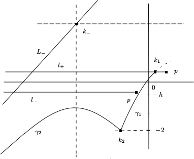
Figure 1. Curves $\gamma_{1}$ and $\gamma_{2}$

If $Y$ is sufficiently big, then (1) the curve $\gamma_{-}$ does stays between $p$ and all the other poles of $v$; (2) its segment $\gamma_{2}$ is located below the poles of the integrand at a distance greater than $1$.
Let us estimate $\int_{\gamma_{1}}I(p)\,dp$. We note that, by the definition of $H_{i}$ and by (4.9), the expression ${\rm Im}\,\left(2kz+k^{2}-k-kh\right)$ is constant on $H_{i}(k_{1})$. By (4.3) we get

(4.19) $$\left|\frac{1}{\sqrt{h}}\int_{\gamma_{1}}e^{\frac{2\pi izk}{h}}v(k)dk\right|\leq\frac{C\left|e^{-\frac{C(H_{i})}{h}}\right|}{\sqrt{h}}\times\\ \times\int_{\gamma_{1}}|\sigma_{\pi h}(2\pi(k+p-{\textstyle\frac{h}{2}-\frac{1}{2}}))\sigma_{\pi h}(2\pi(k-p-{\textstyle\frac{h}{2}-\frac{1}{2}}))dk|$$

where

$$C(H_{i})=\pi\left.{\rm Im}\,\left(2kz+k^{2}-k-kh\right)\right|_{H_{i}(k_{1})},\quad$$

Computing $C(H_{i})$ at the point $k_{1}$, we get

(4.20) $$\left|e^{-\frac{C(H_{i})}{h}}\right|\leq C\,\left|e^{\frac{2\pi ipz}{h}}\right|\,e^{-2\pi\beta|y|}.$$

Let us estimate the integrand in the right hand side of (4.19). Using (2.5), we get

$$\sigma_{\pi h}(2\pi(k-p-{\textstyle\frac{h}{2}-\frac{1}{2}}))=\frac{\sigma_{\pi h}(2\pi(k-p+{\textstyle\frac{h}{2}-\frac{1}{2}}))}{1-e^{-2\pi i(k-p)}}.$$

For $k\in\gamma_{1}$, one has

$$\begin{split}{\rm Re}\,(k+p-h/2-1/2)&\geq-1/2-h/2+2{\rm Re}\,p-\beta h-C(Y)|{\rm Im}\,(k-p)|\\ &\geq-1/2-h/2+(\alpha-\beta)h-C(Y)|{\rm Im}\,(k-p)|,\\ {\rm Re}\,(k-p+h/2-1/2)&\geq-1/2-h/2+(1-\beta)h-C(Y)|{\rm Im}\,(k-p)|.\end{split}$$

where $C(Y)>0$ tends to zero as $Y\to\infty$. These observations and Corollaries 8.1– 8.2 imply that, for sufficiently large $Y$ and $k\in\gamma_{1}$,

$$|\sigma_{\pi h}(2\pi(k+p-{\textstyle\frac{h}{2}-\frac{1}{2}}))\,\sigma_{\pi h}(2\pi(k-p-{\textstyle\frac{h}{2}-\frac{1}{2}}))|\leq H.$$

This estimate and (4.20) imply estimate (4.18) with $\gamma_{1}$ instead of $\gamma_{\pm}$.

Consider the integral $\int_{\gamma_{2}}I(k)\,dk$. As $\gamma_{2}$ stays below the poles of $I$, at a distance greater than $1$, by means of Corollary 8.1, one immediately obtains

$$|\sigma_{\pi h}(2\pi(k+p-{\textstyle\frac{h}{2}-\frac{1}{2}}))\,\sigma_{\pi h}(2\pi(k-p-{\textstyle\frac{h}{2}-\frac{1}{2}}))|\leq H,\quad k\in\gamma_{2},$$

and

$$\left|\int_{\gamma_{2}}I\,dk\right|\leq H\,\left|e^{\frac{\pi i}{h}\,\left.(2kz+k^{2}-k-kh)\right|_{k=k_{2}}}\right|\,\int_{\gamma_{2}}\left|e^{\frac{\pi i}{h}((k-k_{-}(z))^{2}-(k_{2}-k_{-}(z))^{2})}\,dk\right|.$$

Clearly,

$$\left|e^{\frac{\pi i}{h}\left.(2kz+k^{2}-k-kh)\right|_{k=k_{2}}}\right|=e^{-\frac{C(H_{i})}{h}}\leq C\,\left|e^{\frac{2\pi ipz}{h}}\right|e^{-2\pi\beta|y|}.$$

We remind that curve $\gamma_{2}\subset H_{r}(k_{2})$ goes to infinity approaching the asymptote $e^{i\pi/4}(-\infty,0]$. Integrating by parts, we get

$$\int_{\gamma_{2}}\left|e^{\frac{\pi i}{h}((k-k_{-}(z))^{2}-(k_{2}-k_{-}(z))^{2})}\,dk\right|\leq Ch/|k_{2}-k_{-}|.$$

These estimates imply that $\int_{\gamma_{2}}I\,dk$ satisfies an estimate of the form (4.18). This implies (4.18) with $\gamma_{-}$.

The estimates of the integral along $\gamma_{+}$, the part of $\gamma$ above the line ${\rm Im}\,k={\rm Im}\,p$ are similar. We omit the details and mention only that now the role of $e^{i\frac{(k-k_{-}(z))^{2}}{h}}$ is played by the exponential $e^{-i\frac{(k-k_{+}(z))^{2}}{h}}$. The obtained estimates and the formula for $A$ imply (4.15). This completes the proof of (4.15). Representation (4.16) is obtained similarly. ∎

4.4. Rough estimates

We shall need

Lemma 4.1.

Pick $X>0$. Let $p\in P$ and $|x|\leq X$. One has

(4.21) $$|\mu(z)|,\;|\mu^{\prime}(z)|\leq Hw(x,y),\quad w(x,y)=(1+|y|)\begin{cases}e^{\frac{2\pi(|x|-1/2)y}{h}-\pi y},&y\geq 0,\\ e^{\frac{2\pi{\rm Re}\,p|y|}{h}},&y\leq 0.\end{cases}$$

When proving this lemma we use

Lemma 4.2.

Pick $\alpha\in(0,1)$. For $p\in P$ one has

(4.22) $$|a(p)|\leq H\quad\text{if}\quad|p|\geq\alpha h/2,$$

(4.23) $$|a(p)+a(-p)|\leq H,\quad|pa(p)|\leq H\quad\text{if}\quad|p|\leq\alpha h/2.$$

Proof.

Let $|p|\geq\alpha h/2$ and $p\in P$. Corollaries 8.1 and 8.2 imply that $|\sigma_{\pi h}(4\pi p-\pi h-\pi))|\leq H$. This and (4.14) lead to (4.22).

Assume that $|p|\leq\alpha h/2$ ($p$ is not necessarily in $P$). In view of (4.14), it suffices to check that

$$|\sigma_{\pi h}(4\pi p-\pi h-\pi)+\sigma_{\pi h}(-4\pi p-\pi h-\pi)|\leq\frac{C}{h},\quad|p\sigma_{\pi h}(4\pi p-\pi h-\pi)|\leq C.$$

Both the functions $p\mapsto\sigma_{\pi h}(4\pi p-\pi h-\pi)+\sigma_{\pi h}(-4\pi p-\pi h-\pi)$ and $p\mapsto p\sigma_{\pi h}(4\pi p-\pi h-\pi)$ are analytic in $p$ in the $\frac{\alpha h}{2}$-neighborhood of zero (see section 8.1.2). By Theorem 8.2 $\sigma_{\pi h}(2\pi(2p-{\textstyle\frac{h}{2}-\frac{1}{2}}))$ is bounded by $C/h$ at the boundary of this neighborhood. This and the maximum principle imply the needed estimates. ∎

Now we can check Lemma 4.1.

Proof.

Let $p\in P$. Pick $Y$ sufficiently large. For $y\geq-Y$, the estimate for $\mu$ follows directly from Proposition 4.1. For $|y|\leq Y$, the estimate for $\mu^{\prime}$ follows from the estimate for $\mu$ and the Cauchy estimates for the derivatives of analytic functions (as $X$ and $Y$ were chosen rather arbitrarily). Let $y\geq Y$ and $|x|\leq X$. The first estimate in (4.21) implies that, in the $(h/y)$-neighborhood of $z$, $\mu$ is bounded by $Hw(x,y)$ (we again use the fact that $X$ and $Y$ were chosen rather arbitrarily). This and the Cauchy estimates for the derivatives of analytic functions lead then to the estimate $|\mu^{\prime}(z)|\leq yHw(x,y)$. This completes the proof of (4.21) for $y\geq-Y$.

Let us prove (4.21) for $y\leq-Y$. Pick $0<\alpha<1$. Let $|x|\leq X$,   $y\leq-Y$ and ${\rm Re}\,p\geq\alpha h/2$. Estimate (4.22) and Proposition 4.2 imply that

(4.24) $$|\mu(z)e^{-\frac{2\pi ipz}{h}}|\leq H.$$

By means of the Cauchy estimates for the derivatives of analytic functions we get the estimate

(4.25) $$\left|\frac{d}{dz}(\mu(z)e^{-\frac{2\pi ipz}{h}})\right|\leq H.$$

Estimates (4.24)–(4.25) lead to (4.21) for $|x|\leq X$, $y\leq-Y$ and ${\rm Re}\,p\geq\alpha h/2$. If $0\leq{\rm Re}\,p\leq\alpha h/2$, the estimates for $\mu$ and its derivative are deduced from (4.16) and (4.23) similarly. We omit further details. ∎

4.5. One more solution to the model equation

Let

(4.26) $$\tilde{\mu}\,(z,p)=e^{-i\pi z/h}\,\mu\,(z+1/2,1/2-p),$$

were we indicate the dependence of $\mu$ on $p$ explicitly. Together with $\mu$,  $\tilde{\mu}$ is a solution to (4.1). It is entire in $z$ and $p$. We use it to construct entire solutions to the Harper equation. Here, we compute the Wronskian $\{\mu,\,\tilde{\mu}\}=\mu(z+h)\tilde{\mu}(z)-\mu(z)\tilde{\mu}(z+h)$.

Lemma 4.3.

For all $p\in{\mathbb{C}}$,

(4.27) $$\{\mu,\,\tilde{\mu}\}=ie^{-\frac{2\pi ip^{2}}{h}-\frac{i\pi}{12h}-\frac{\pi ih}{3}}.$$

Proof.

Pick $X>0$ and $0<\alpha<\frac{1}{2}$. Assume that $\alpha h/2\leq p\leq 1/2-\alpha h/2$. Then, by means of (4.26), (4.15) and (4.22), we check that, uniformly in $x\in[-X,X]$, as $y\to-\infty$ the Wronskian $\{\mu,\,\tilde{\mu}\}$ tends to

(4.28) $$2ie^{\frac{i\pi}{2h}-\frac{i\pi p}{h}}\,a(1/2-p)a(p)\sin(2\pi p).$$

By means of (4.21), we check that, as $y\to+\infty$, uniformly in $x\in[-h,0]$,

$$|\{\mu(z),\,\tilde{\mu}(z)\}|\leq H|y|\left(e^{\frac{2\pi y}{h}(x-\frac{1}{2}+|x+1/2|)}+1\right)\leq H|y|.$$

The Wronskian being entire (as $\mu$ and $\tilde{\mu}$) and $h$-periodic in $z$ (as the Wronskian of any two solutions to a one-dimensional difference Schrödinger equation, see section 3.1.3), we conclude that it is independent of $z$ and equals the expression in (4.28). As the Wronskian is entire in $p$, this statement is valid for all $p$. Finally, using the definition of $a$, equation (2.5) and formula (8.3), we check that

(4.29) $$2i\,a(1/2-p)a(p)\sin(2\pi p)=ie^{-\frac{2\pi ip^{2}}{h}+\frac{i\pi p}{h}-\frac{7i\pi}{12h}-\frac{\pi ih}{3}}.$$

This leads to the statement of the lemma. ∎

5. Analytic solution to Harper equation

5.1. Preliminaries

For $Y\in{\mathbb{R}}$, we set ${\mathbb{C}}_{+}(Y)=\{y>Y\}$. Here, we pick $Y>0$ and for sufficiently small $\lambda>0$ construct a solution to (2.1) analytic in ${\mathbb{C}}_{+}(-Y)$.

Below, we represent the spectral parameter $E$ in the form $E=2\cos(2\pi p)$ and consider solutions to (2.1) as functions of the parameter $p$.

As $\lambda$ is small, then, when constructing solutions to (2.1) in ${\mathbb{C}}_{+}(-Y)$, it is natural to rewrite this equation in the form

(5.1) $$\psi\,(z+h)+\psi\,(z-h)+\lambda\,e^{-2\pi iz}\psi\,(z)-2\cos(2\pi p)\,\psi(z)=-\lambda\,e^{2\pi iz}\,\psi(z),$$

so that the term in the right hand side could be considered as a perturbation. Let $\xi=\frac{1}{2\pi}\ln\lambda$. Then $\mu(z+i\xi)$ is a solution to the unperturbed equation

(5.2) $$\psi\,(z+h)+\psi\,(z-h)+\lambda\,e^{-2\pi iz}\psi\,(z)-2\cos(2\pi p)\,\psi(z)=0.$$

We construct $\psi$, an analytic solution to equation (5.1) close to $\mu(z+i\xi)$. We prove

Theorem 5.1.

Pick positive $Y$. There exists $C$ such that if  $\lambda\leq e^{-\frac{C}{h}}$,  then:

$\bullet$   There is $\psi_{0}$, a solution to (2.1) analytic in $(z,p)\in{\mathbb{C}}_{+}(-Y)\times P$;

$\bullet$   Pick positive $X$. As $y\to+\infty$, uniformly in $x\in[-X,X]$

(5.3) $$\psi_{0}(z)=e^{\frac{i\pi}{4}}\,\xi_{-}(z+i\xi)\,v_{-}\,(1+\varkappa_{0}+o(1))-e^{-\frac{i\pi}{4}}\,\xi_{+}(z+i\xi)\,v_{+}\,(1+o(1)),$$

where $\varkappa_{0}$ is a constant satisfying the estimate

$$\textstyle|\varkappa_{0}|\leq H\lambda^{1+\nu(p)}(1+|\xi|)^{3},\quad\nu(p)=\min\left\{1,\frac{1-2{\rm Re}\,p}{h}\right\}.$$

$\bullet$   Fix $X>0$. For $|x|\leq X$ and $y\leq Y/2$, one has

(5.4) $$|\psi_{0}(z)-\mu(z+i\xi)|\leq H\lambda(1+|\xi|)^{3}\,e^{2\pi{\rm Re}\,p|\xi|/h}.$$

The rest of the section is devoted to the proof of Theorem 5.1.

Let us explain the idea of the proof of Theorem 5.1. Let $\gamma=\{z\in i{\mathbb{R}}\,:\,y\geq-Y\}$. We study the integral equation

(5.5) $$\psi\,(z)=\mu\,(z+i\xi)-(K\psi)(z),\quad K\psi(z)=\int_{\gamma}\kappa\,(z,\,z^{\prime})\psi\,(z^{\prime})\,dz^{\prime},\quad z\in\gamma.$$

The kernel $\kappa$ is constructed in terms of $\mu(\cdot+i\xi)$ and $\tilde{\mu}(\cdot+i\xi)$, two linearly independent solutions to the unperturbed equation (5.2),

$$\kappa\,(z,\,z^{\prime})=\frac{\lambda}{2ih}\,\Theta\,(z,\,z^{\prime})\,\frac{[\,\mu(z+i\xi)\,\tilde{\mu}\,(z^{\prime}+i\xi)-\mu\,(z^{\prime}+i\xi)\,\tilde{\mu}\,(z+i\xi)\,]}{\{\mu,\,\tilde{\mu}\}}\,e^{2\pi iz^{\prime}},$$

$$\Theta\,(z,\,z^{\prime})={\mathrm{c}ot}\,\frac{\pi(z^{\prime}-z)}{h}\,-i.$$

Similar integral operators have appeared in [5]. The kernel $\kappa$ can be considered as a difference analog of the resolvent kernel arising in the theory of differential equations. First, we construct a solution to the integral equation (5.5), and then, we check that it is analytic in $z$ and satisfies the difference equation (2.1). Finally, we obtain the asymptotics of this solution for $y\to+\infty$ and for $y\sim 0$.

5.2. Integral equation

Here, we prove the existence of a solution (continuous in $z$ and analytic in $p$) to the integral equation. Below,

$$q(y)=(1+|y|)\begin{cases}e^{-\frac{\pi y}{h}-\pi y},&y\geq 0,\\ e^{\frac{2\pi{\rm Re}\,p|y|}{h}},&y\leq 0,\end{cases}\quad\tilde{q}(y)=(1+|y|)\begin{cases}e^{+\frac{\pi y}{h}-\pi y},&y\geq 0,\\ e^{-\frac{2\pi{\rm Re}\,p|y|}{h}},&y\leq 0.\end{cases}$$

5.2.1. Estimates of $\mu$ and $\tilde{\mu}$

To estimate the norm of the integral operator, we use

Corollary 5.1.

On the curve $\gamma$, the functions $\mu$ and $\tilde{\mu}$ satisfy the estimates

(5.6) $$|\mu(z)|,\,|\mu^{\prime}(z)|\leq Hq(y),\qquad|\tilde{\mu}(z)|,\,|\tilde{\mu}^{\prime}(z)|\leq H\tilde{q}(y),$$

This Corollary follows directly from Lemma 4.1.

5.2.2. A solution to the integral equation

One has

Proposition 5.1.

Fix positive $\alpha<1$. There is a positive constant $C$ such that if $\lambda\leq e^{-\frac{C}{h}}$, then the integral equation (5.5) has a solution $\psi_{0}$ continuous in $z\in\gamma$, analytic in $p\in P$ and satisfying the estimate

(5.7) $$\left|\psi_{0}(z)-\mu(z+i\xi)\right|\leq\lambda^{\alpha}Hq(y+\xi),\quad z\in\gamma.$$

Proof.

Let $C(\gamma,q)$ be the space of functions defined and continuous on $\gamma$ and having the finite norm $\|f\|=\sup_{z\in\gamma}|q^{-1}(y+\xi)\,f(z)|$. The proof is based on

Lemma 5.1.

For $z,\,z^{\prime}\in\gamma$, one has

(5.8) $$|q^{-1}(y+\xi)\,\kappa\,(z,\,z^{\prime})\,q(y^{\prime}+\xi)|\leq\lambda\,H\,e^{-2\pi y^{\prime}}(1+\xi^{2}).$$

First, we prove the proposition, and then, we check estimate (5.8). This estimate implies that the norm of $K$ as an operator acting in $C(\gamma,q)$ is bounded by $\lambda\,H\,(1+\xi^{2})$. By Corollary 5.1, $\mu(.+\xi)\in C(\gamma,q)$. So, there is a positive constant $C$ such that, if $\lambda(1+\xi^{2})\,<e^{-C/h}$, then there is $\psi_{0}$, a solution to (5.5) from $C(\gamma,q)$. The estimate of the norm of the integral operator implies that

$$\left|\psi_{0}(z)-\mu(z)\right|\leq\lambda(1+\xi^{2})Hq(y+\xi),\quad z\in\gamma.$$

This implies (5.7) for any fixed positive $\alpha<1$. The analyticity of $\psi_{0}$ in $p$ follows from one of $\mu$ and the uniformity of the estimates. The proof is complete.∎

Let us prove Lemma 5.1. Below, $z,z^{\prime}\in\gamma$. We note that by (4.27), for $p\in P$ one has $C^{-1}\leq\{\mu(z),\tilde{\mu}(z)\}\leq C$.

First, we consider the case where $|y-y^{\prime}|\geq h$. In view of Corollary 5.1, we get

$$|q^{-1}(y+\xi)\,\kappa\,(z,\,z^{\prime})\,q(y^{\prime}+\xi)|\leq\lambda He^{-2\pi y^{\prime}}(E_{1}+E_{2}),$$

$$E_{1}=|\Theta(z,z^{\prime})|\,\tilde{q}(y^{\prime}+\xi)\,q(y^{\prime}+\xi),\qquad E_{2}=|\Theta(z,z^{\prime})|\,\frac{\tilde{q}(y+\xi)}{q(y+\xi)}\,q^{2}(y^{\prime}+\xi).$$

To justify (5.8), it suffices to check that $E_{1,2}\leq C\,(1+|\xi|)^{2}$. Note that

(5.9) $$|\Theta(z,z^{\prime})|\leq C\,\begin{cases}e^{-\frac{2\pi(y-y^{\prime})}{h}}&\text{ if }y-y^{\prime}\geq h,\\ 1&\text{ if }y^{\prime}-y\geq h.\end{cases}$$

Clearly, $E_{1}\leq C\,\tilde{q}(y^{\prime}+\xi)q(y^{\prime}+\xi)$. For $y^{\prime}\geq-Y$, we have

(5.10) $$\begin{split}\tilde{q}(y^{\prime}+\xi)q(y^{\prime}+\xi)&\leq(1+|y^{\prime}+\xi|)^{2}e^{-2\pi(y^{\prime}+\xi)}\leq C,\quad\text{if}\quad y^{\prime}+\xi\geq 0,\\ \tilde{q}(y^{\prime}+\xi)q(y^{\prime}+\xi)&\leq(1+|y^{\prime}+\xi|)^{2}\leq C\,(1+|\xi|)^{2}\quad\text{otherwise}.\end{split}$$

This implies that $E_{1}\leq C\,(1+|\xi|)^{2}$. To estimate $E_{2}$, we have to consider four cases. If $y+\xi,\,y^{\prime}+\xi\geq 0$, we have

$$E_{2}\leq|\Theta(z,z^{\prime})|\,(1+|y^{\prime}+\xi|)^{2}\,e^{\frac{2\pi(y-y^{\prime})}{h}-2\pi(y^{\prime}+\xi)}\leq C\,|\Theta(z,z^{\prime})|\,e^{\frac{2\pi(y-y^{\prime})}{h}}\leq C.$$

If $y+\xi\geq 0\geq y^{\prime}+\xi$, then

$$\begin{split}E_{2}\leq(1+|y^{\prime}+\xi|)^{2}\,&|\Theta(z,z^{\prime})|\,e^{\frac{2\pi(y+\xi)}{h}-\frac{4\pi{\rm Re}\,p(y^{\prime}+\xi)}{h}}\\ &\leq C\,(1+\xi^{2})\,e^{\frac{2\pi(1-2{\rm Re}\,p)(y^{\prime}+\xi)}{h}}\leq C\,(1+\xi^{2}).\end{split}$$

If $y^{\prime}+\xi\geq 0\geq y+\xi$, then

$$\begin{split}E_{2}\leq(1+|&y^{\prime}+\xi|)^{2}\,|\Theta(z,z^{\prime})|\,e^{\frac{4\pi{\rm Re}\,p(y+\xi)}{h}-\frac{2\pi(y^{\prime}+\xi)}{h}-2\pi(y^{\prime}+\xi)}\\ &\leq C\,|\Theta(z,z^{\prime})|\,e^{\frac{4\pi{\rm Re}\,p(y+\xi)}{h}-\frac{2\pi(y^{\prime}+\xi)}{h}}\leq C\,|\Theta(z,z^{\prime})|\leq C.\end{split}$$

Finally, if $y+\xi,\,y^{\prime}+\xi\leq 0$, we get

$$E_{2}\leq(1+|y^{\prime}+\xi|)^{2}\,|\Theta(z,z^{\prime})|\,e^{\frac{4\pi{\rm Re}\,p(y-y^{\prime})}{h}}\leq C\,(1+|\xi|)^{2}.$$

These estimates imply that $E_{2}\leq C\,(1+|\xi|)^{2}$. This completes the proof in the case where $|y-y^{\prime}|\geq h$.
Let us consider the case where $|y-y^{\prime}|\leq h$. Let $\eta={\rm Im}\,\zeta$. Using (4.21) we get

$$\begin{split}|\Theta(z,z^{\prime})\,(\mu(z+i&\xi)\,\tilde{\mu}\,(z^{\prime}+i\xi)-\mu\,(z^{\prime}+i\xi)\,\tilde{\mu}\,(z+i\xi)\,)|\\ &\leq Ch\,\max_{\zeta\in\gamma,\,|y-\eta|\leq h}\left|\mu(z+i\xi)\,\tilde{\mu}^{\prime}(\zeta+i\xi)-\mu^{\prime}(\zeta+i\xi)\,\tilde{\mu}\,(z+i\xi)\right|\\ &\leq H\left(q(y+\xi)\max_{|y-\eta|\leq h}\tilde{q}(\eta+\xi)+\tilde{q}(y+\xi)\max_{|y-\eta|\leq h}q(\eta+\xi)\right)\\ &\leq Hq(y+\xi)\tilde{q}(y+\xi),\end{split}$$

and, using (5.10), we again come to (5.8). This completes the proof. ∎

Note that Corollary 5.1 and Proposition 5.1 imply

Corollary 5.2.

In the case of Proposition 5.1, there is $C$ such that, for $\lambda\leq e^{-\frac{C}{h}}$,

(5.11) $$|\psi_{0}(z)|\leq Hq(y+\xi),\quad z\in\gamma.$$

5.3. Analytic continuation of the solution to the integral equation

Here, we prove the first point of Theorem 5.1. One has

Lemma 5.2.

The solution $\psi_{0}$ can be analytically continued in ${\mathbb{C}}_{+}(-Y)$.

Similar statements were checked in [5] and [6], we outline the proof only for the convenience of the reader.

Proof.

For $z^{\prime}\in\gamma$, the kernel $\kappa\,(z,\,z^{\prime})$ is analytic in $z\in S_{h}=\{|{\rm Re}\,z|<h,\,y>-Y\}$, and the function $K\psi_{0}$ can be analytically continued in $S_{h}$;   $\psi_{0}$, being a solution to (5.5), can be also analytically continued in $S_{h}$.

Having proved that $\psi_{0}$ is analytic in $S_{h}$, one can deform the integration contour in the formula for $K\psi_{0}$ inside $S_{h}$, and check that, in fact, $\psi_{0}$ can be analytically continued in $S_{2h}=\{|{\rm Re}\,z|<2h,y>-Y\}$. Continuing in this way, one comes to the statement of the Lemma. ∎

Below, we denote by $\psi_{0}$ also the analytic continuation of the old $\psi_{0}$.

5.3.1. Function $\psi_{0}$ and the difference equation

To check that $\psi_{0}$ satisfies (5.1), we again borrow an argument from [5] and [6].

We call a curve in ${\mathbb{C}}$ vertical if along it $x$ is a smooth function of $y$. For $z\in{\mathbb{C}}_{+}(-Y)$ we denote by $\gamma(z)$ a vertical curve that begins at $-iY$, goes upward to $z$, then comes back to the imaginary axis and goes along it to $+i\infty$. One can compute $K\psi_{0}(z)$ by the formula in (5.5) with the integration path $\gamma$ replaced with $\gamma(z)$.

Set $({\mathcal{H}}_{0}\,f)\,(z)=f\,(z+h)+f\,(z-h)+\lambda\,e^{-2\pi iz}f(z)-2\cos(2\pi p)\,f(z)$. Then, ${\mathcal{H}}_{0}\,\psi_{0}=-{\mathcal{H}}_{0}\,K\psi_{0}$. Using (5.5) with $\gamma$ replaced with $\gamma(z)$,  $z\in{\mathbb{C}}_{+}(-Y)$, we get

$$({\mathcal{H}}_{0}\,K\,\psi_{0})\,(z)=2\pi i\;{\rm res}\,_{z^{\prime}=z}\,\kappa\,(z+h,\,z^{\prime})\,\psi_{0}(z^{\prime})=\lambda\,e^{2\pi iz}\,\psi_{0}(z).$$

Thus, we come to

Lemma 5.3.

The solution $\psi_{0}$ satisfies equation (2.1) in ${\mathbb{C}}_{+}(-Y)$.

The last two lemmas imply the first point of the Theorem 5.1.

5.4. Asymptotics in the upper half-plane

We get asymptotics (5.3) using the integral equation for $\psi_{0}$. First, we pick $\delta\in(0,1)$ and sufficiently large $Y>0$, assume that $|x|\leq\delta h$ and $y>Y$, and represent $(K\psi_{0})(z)$ in the form

(5.12) $$(K\psi_{0})(z)=\textstyle\frac{\lambda}{2ih\{\mu,\,\tilde{\mu}\}}\,\left(\mu\,(z+i\xi)(I(\tilde{\mu})+J(\tilde{\mu}))-\tilde{\mu}\,(z+i\xi)(I(\mu)+J(\mu))\right),$$

where

(5.13) $$I(f)=\int_{\gamma,\,\,|y-y^{\prime}|\geq h}\Theta\,(z,\,z^{\prime})\,f\,(z^{\prime}+i\xi)\,e^{2\pi iz^{\prime}}\,\psi_{0}(z^{\prime})dz^{\prime},$$

(5.14) $$J(f)=\int_{\gamma,\,\,|y-y^{\prime}|\leq h}\Theta\,(z,\,z^{\prime})\,(f\,(z^{\prime}+i\xi)-f(z+i\xi))\,e^{2\pi iz^{\prime}}\,\psi_{0}(z^{\prime})dz^{\prime}.$$

Let us estimate $I(\mu)$, $I(\tilde{\mu})$, $J(\mu)$ and $J(\tilde{\mu})$. The first two are defined $\forall x$. One has

Lemma 5.4.

Let $p\in P$. We pick $X>0$. As $y\to+\infty$, uniformly in $x\in[-X,X]$

(5.15) $$I(\tilde{\mu})(z)=o(1),\qquad I(\mu)(z)=e^{\frac{2\pi i(z+i\xi)}{h}}(a+o(1)),$$

where

(5.16) $$a=2i\int_{\gamma}e^{-\frac{2\pi i(z^{\prime}+i\xi)}{h}}\mu\,(z^{\prime}+i\xi)\,e^{2\pi iz^{\prime}}\,\psi_{0}(z^{\prime})dz^{\prime}.$$

One has

(5.17) $$a=O\left((1+|\xi|)^{3}\lambda^{\nu(p)}H\right),\quad\textstyle\nu(p)=\min\left\{1,\frac{1-2{\rm Re}\,p}{h}\right\}.$$

Note that the integral in (5.16) converges in view of (5.6) and (5.11).

Proof.

Let us estimate $I(\tilde{\mu})$. We assume that $y+\xi>0$. Using (5.9),  (5.6) and (5.11), we get

$$|I(\tilde{\mu})(z)|\leq H\left(\int_{y}^{\infty}(1+|y^{\prime}+\xi|)^{2}e^{-2\pi(y^{\prime}+\xi)}e^{-2\pi y^{\prime}}dy^{\prime}\right.\\ \hskip 85.35826pt+\int_{-\xi}^{y}e^{-\frac{2\pi(y-y^{\prime})}{h}}(1+|y^{\prime}+\xi|)^{2}e^{-2\pi(y^{\prime}+\xi)}e^{-2\pi y^{\prime}}dy^{\prime}\\ \left.+\int_{-Y}^{-\xi}e^{-\frac{2\pi(y-y^{\prime})}{h}}(1+|y^{\prime}+\xi|)^{2}e^{-2\pi y^{\prime}}dy^{\prime}\right).$$

The expression in the brackets is bounded by

$$\int_{y}^{\infty}e^{-2\pi y^{\prime}}dy^{\prime}+\int_{-\xi}^{y}e^{-\frac{2\pi(y-y^{\prime})}{h}}e^{-2\pi y^{\prime}}dy^{\prime}+(1+|Y-\xi|^{2})\int_{-Y}^{-\xi}e^{-\frac{2\pi(y-y^{\prime})}{h}}e^{-2\pi y^{\prime}}dy^{\prime}.$$

As $h<1$, this implies the first estimate from (5.15).
Let us turn to $I(\mu)$. Arguing as when estimating $I(\tilde{\mu})$, we check that

(5.18) $$\left|\int_{\gamma,\,\,y^{\prime}>y+h}\Theta\,(z,\,z^{\prime})\,\mu\,(z^{\prime}+i\xi)\,e^{2\pi iz^{\prime}}\,\psi_{0}(z^{\prime})dz^{\prime}\right|\leq\\ \leq H\int_{y+h}^{\infty}(1+|y^{\prime}+\xi|)^{2}e^{-\frac{2\pi(y^{\prime}+\xi)}{h}-2\pi(y^{\prime}+\xi)}e^{-2\pi y^{\prime}}dy^{\prime}=o(e^{-\frac{2\pi y}{h}})$$

uniformly in $x$ as $y\to+\infty$. Then, using the estimate

$$\left|\Theta(z,z^{\prime})-2ie^{-\frac{2\pi i(z^{\prime}-z)}{h}}\right|\leq Ce^{-\frac{4\pi(y-y^{\prime})}{h}},\quad y-y^{\prime}\geq h,$$

and again arguing as before, we prove that as $y\to\infty$, uniformly in $x$

(5.19) $$\operatornamewithlimits{\int}_{\gamma,\,\,y>y^{\prime}+h}\Theta\,(z,\,z^{\prime})\,\mu\,(z^{\prime}+i\xi)\,e^{2\pi iz^{\prime}}\,\psi_{0}(z^{\prime})dz^{\prime}=e^{\frac{2\pi i(z+i\xi)}{h}}a+o\left(e^{-\frac{2\pi y}{h}}\right)$$

with $a$ from (5.16). Estimates (5.18)–(5.19) imply the second estimate in (5.15).

Let us prove (5.17). Using (5.16) and estimates (5.6) and (5.11), we get

$$|a|\leq H(1+|\xi|)^{2}\operatornamewithlimits{\int}_{-Y}^{-\xi}e^{\frac{2\pi(1-2{\rm Re}\,p)(y^{\prime}+\xi)}{h}-2\pi y^{\prime}}dy^{\prime}+H\operatornamewithlimits{\int}_{-\xi}^{+\infty}e^{-2\pi(2y^{\prime}+\xi)}(1+|y^{\prime}+\xi|)^{2}dy^{\prime}.$$

One has $\max_{0\leq y^{\prime}\leq-\xi}e^{\frac{2\pi(1-2{\rm Re}\,p)(y^{\prime}+\xi)}{h}-2\pi y^{\prime}}=e^{2\pi\nu(p)\xi}=\lambda^{\nu(p)}$ with $\nu(p)$ defined by the second formula in (5.17). Furthermore, the second integral in the last estimate for $a$ equals $\lambda\int_{0}^{+\infty}e^{-4\pi t}(1+t)^{2}dt$. These observations lead to (5.17). This completes the proof of the lemma. ∎

Let us turn to the terms $J(\mu)$ and $J(\tilde{\mu})$. One has

Lemma 5.5.

Fix $\delta\in(0,1)$. Let $p\in P$. As $y\to+\infty$, one has

(5.20) $$J(\tilde{\mu})(z)=o(1),\quad J(\mu)(z)=o(e^{-\frac{2\pi y}{h}}).$$

These estimates are uniform in $x\in[-\delta h,\delta h]$.

Proof.

Let $y+\xi\geq h$. Using estimates (4.21) for $d\mu/dz$ and estimate (5.11), we get

$$|J(\mu)|\leq H(1+|y+\xi|)^{2}e^{2\pi\delta(y+\xi)-\frac{2\pi(y+\xi)}{h}-2\pi(y+\xi)-2\pi y}(1+|y+\xi|)^{2}\leq He^{-\frac{2\pi(y+\xi)}{h}-2\pi y},$$

where we used the inequalities $|x|\leq\delta h$ and $0<\delta<1$. This implies the first estimate in (5.20). Similarly one proves the second one. ∎

Now we are ready to prove (5.3). We do it in three steps. Below we assume that $p\in P$. All the $o(1)$ are uniform in $x$.
1.   Fix $\delta\in(0,1)$. Let $|x|\leq\delta h$. Estimates (5.15) and (5.20) imply that as $y\to\infty$

(5.21) $$\psi_{0}=\mu(z+i\xi)-(K\psi_{0})(z)=\mu(z+i\xi)(1+o(1))+e^{\frac{2\pi i(z+i\xi)}{h}}\tilde{\mu}(z+i\xi)(\tilde{a}+o(1))$$

where $\tilde{a}=\lambda a/(2hi\{\mu,\,\tilde{\mu}\})$. Representation (5.21), and formulas (4.26) and (4.7) imply (5.3) with $\varkappa_{0}=ie^{\frac{i\pi}{4h}}\tilde{a}$. This completes the proof of (5.3) for $x\in[-\delta h,\delta h]$. We note that (5.3) implies that, for sufficiently large $y$,

(5.22) $$|\psi_{0}(z)|\leq C(1+|\varkappa_{0}|)e^{\frac{2\pi|x|(y+\xi)}{h}-\frac{\pi(y+\xi)}{h}-\pi(y+\xi)}.$$

2.   Now, we pick $\delta\in(1/2,1)$ and justify (5.3) assuming that $h\delta\leq x\leq h(1+\delta)$. Let $\epsilon\in(0,1-\delta)$. We denote by $\gamma(z)$ the curve that goes first along a straight line from $i(y-h)$ to the point $z-h+\epsilon h$ and next along a straight line from this point to $i(y+h)$. One obtains representation (5.12) with $J(f)$ defined by the new formula:

(5.23) $$J(f)(z)=\int_{\gamma(z)}\Theta\,(z,\,z^{\prime})\,f\,(z^{\prime}+i\xi)\,e^{2\pi iz^{\prime}}\,\psi_{0}(z^{\prime})dz^{\prime}.$$

We note that on $\gamma(z)$, one has $|\Theta\,(z,\,z^{\prime})|\leq C$. As

$$-\delta h\leq(\delta-1)h<x-h+\epsilon h\leq(\delta+\epsilon)h,$$

and as $\delta+\epsilon<1$, we can and do assume that on $\gamma(z)$ for sufficiently large $y$ solution $\psi_{0}$ satisfies (5.22). Using (5.22) and (4.21), we check that as $y\to+\infty$

$$|J(\mu)(z)|\leq H(1+|\varkappa_{0}|)e^{4\pi(\delta+\epsilon-1)(y+\xi)-\frac{2\pi(y+\xi)}{h}+2\pi\xi}(1+|y+\xi|)^{2}=o(e^{-\frac{2\pi(y+\xi)}{h}}).$$

Reasoning analogously, we also prove that $J(\tilde{\mu})(z)=o(1)$ as $y\to+\infty$. These two estimates and (5.15) lead again to (5.3). This completes the proof of (5.3) for $0\leq x\leq(1+\delta)h$. The case of $(1+\delta)h\leq x\leq 0$ is analyzed similarly.
3.  To justify (5.3) for larger $|x|$, one uses equation (5.1). We discuss only the case of $x\geq 0$ and omit further details. Pick $\delta\in(0,1)$ and $X>0$. In the case of Theorem 5.3, we can assume that $|\varkappa_{0}|\leq 1/2$. Then, $1+\varkappa_{0}\neq 0$ and for $x\in[\delta h,X]$ (5.3) actually means that

$$\psi_{0}(z)=A\xi_{-}(z+i\xi)(1+o(1)),\qquad A=e^{\frac{i\pi}{4}}(1+\varkappa_{0})v_{-}\,.$$

By (5.1), one can write

$$\psi_{0}(z)=-\lambda e^{-2\pi i(z-h)}\psi_{0}(z-h)\,\left(1+o(1)+e^{2\pi i(z+i\xi-h)}\,\psi_{0}(z-2h)/\psi_{0}(z-h)\right).$$

Let $(1+\delta)h\leq x\leq(2+\delta)h$. Then $\psi_{0}(z-h)=A\xi_{-}(z+i\xi-h)(1+o(1))$. This and (5.22) (that is valid on any given compact subinterval of $(-h,h)$) imply that $e^{2\pi iz}\psi_{0}(z-2h)/\psi_{0}(z-h)=o(1)$. Therefore,

$$\psi_{0}(z)=-\lambda\,e^{-2\pi i(z-h)}\psi_{0}(z-h)\,(1+o(1))=A\xi_{-}(z+i\xi)(1+o(1)).$$

So, we proved (5.3) for $x\in[0,(2+\delta)h]$. Continuing in this way, one proves (5.3) for all $x$ such that $0\leq x\leq X$. This completes the proof of (5.3).∎

5.5. Asymptotics in the lower half-plane

Here, we prove the third statement of Theorem 5.1, i.e., estimate (5.4). We pick $X>0$ and a sufficiently large $Y>0$ and assume that $|x|\leq X$ and $|y|\leq Y/2$. We also assume that $\lambda$ is so small (or $\lambda\leq e^{C/h}$ with $C$ so large) that $Y<-\xi$.

The proof follows the same plan and uses the same estimates for $\mu$, $\tilde{\mu}$ and $\psi_{0}$ as for studying $\psi_{0}$ as $y\to\infty$. So, we omit elementary details.
1.  First, we represent $K\psi_{0}$ in the form (5.12) with $I$ and $J$ given by (5.13)– (5.14). Then, using (5.6) and (5.11) and the rough estimate $|\Theta(z,z^{\prime})|\leq C$ for $|y-y^{\prime}|\geq h$, we get

(5.24) $$|I(\tilde{\mu})(z)|\leq H(1+|\xi|)^{2},\quad|I(\mu)(z)|\leq H(1+|\xi|)^{2}\,e^{4\pi{\rm Re}\,p|\xi|/h}.$$

2.  Let us turn to the terms $J(\mu)$ and $J(\tilde{\mu})$. We first fix a positive $\delta<1$, and consider the case where $|x|\leq\delta h$. By means of Lemma 4.1 and (5.11) , we get

(5.25) $$|J(\tilde{\mu})(z)|\leq H\,(1+|\xi|)^{2},\quad|J(\mu)(z)|\leq H\,(1+|\xi|)^{2}\,e^{4\pi{\rm Re}\,p|\xi|/h}.$$

3. We recall that $\psi_{0}(z)-\mu(z+i\xi)=K\psi_{0}(z)$. Estimating the right hand side by means of (5.24)–(5.25), the estimate from Lemma 4.1 for $\mu$ and (4.26), the definition of $\tilde{\mu}$, we get

(5.26) $$|\psi_{0}(z)-\mu(z+i\xi)|\leq\lambda H(1+|\xi|)^{3}\,e^{2\pi{\rm Re}\,p|\xi|/h},$$

i.e., representation (5.4) for $|x|\leq\delta h$
4.  Now, we pick $\delta\in(1/2,1)$ and justify (5.26) for $|x|\leq(1+\delta)h$.
As $|y|<Y/2$, we can assume that the point $z-h$ is above the lower end of $\gamma$. This allows to choose the curve $\gamma(z)$ as in section 5.4, and redefine $J$ by (5.23).

We can and do assume that estimate (5.26) is proved on $\gamma(z)$. This estimate and (4.21) imply that on $\gamma(z)$ one has $|\psi_{0}(z)|\leq H(1+|\xi|)e^{2\pi{\rm Re}\,p|\xi|/h}$. Using this and (4.21) we obtain for the new $J(\mu)$ and $J(\tilde{\mu})$ the old estimates (5.25), and, therefore, we come to (5.26) for $\delta h\leq x\leq(1+\delta)h$. The case of negative $x$ is treated similarly.
5.  Let us prove (5.26) for all $|x|\leq X$. Therefore, we use a difference analog of the Grönwall’s inequality. We discuss only the case where $x>0$. The case of $x<0$ is treated similarly.

Let $\delta(z)=\psi_{0}(z)-\mu(z+i\xi)$. Equations (2.1) and (4.1) for $\psi_{0}$ and $\mu$ imply that

$$\delta(z+h)+\delta(z-h)+2(\lambda\cos(2\pi z)-\cos(2\pi p))\delta(z)=-\lambda e^{2\pi iz}\mu(z+i\xi).$$

Therefore,

$$\Delta(z+h)=M(z)\Delta(z)-\lambda e^{2\pi iz}\mu(z+i\xi)\,e_{1},$$

where

$$\Delta(z)=\begin{pmatrix}\delta(z)\\ \delta(z-h)\end{pmatrix},\quad M(z)=\begin{pmatrix}2(\cos(2\pi p)-\lambda\cos(2\pi z))&-1\\ 1&0\end{pmatrix},\quad e_{1}=\begin{pmatrix}1\\ 0\end{pmatrix}.$$

Let $n(z)=\|\Delta(z)\|_{{\mathbb{C}}^{2}}$ and $A=\max_{|y|\leq Y}\|M(z)\|$, where $\|\cdot\|$ is the Hilbert-Schmidt norm. In view of (4.21) we obtain

(5.27) $$n(z)\leq B+A\,n(z-h),\quad B=\lambda(1+|\xi|)He^{2\pi{\rm Re}\,p|\xi|/h}.$$

Therefore, for $N\in{\mathbb{N}}$, we have

(5.28) $$n(z)\leq B\,(1+A+...A^{N-1})+A^{N}\,n(z-Nh)=B\frac{A^{N}-1}{A-1}+A^{N}\,n(z-Nh).$$

Assume that $\frac{3h}{2}\leq x\leq X$ and choose $N$ so that $\frac{h}{2}\leq x-Nh\leq\frac{3h}{2}$. Then,
$\bullet$   by (5.26),  $n(z-Nh)\leq\lambda H(1+|\xi|)^{3}\,e^{2\pi{\rm Re}\,p|\xi|/h}$;
$\bullet$  $1\leq N\leq C/h$, and $A^{N}\leq H$.
Using these observations and the estimate for $B$ from (5.27), we deduce from (5.28) estimate (5.26) for $0\leq x\leq X$. This completes the proof of Theorem 5.1.

6. A monodromy matrix for the Harper equation

Here we give a definition of the minimal entire solutions to the Harper equation and describe the monodromy matrix corresponding to a basis of two minimal entire solutions. This is the matrix described in Theorem 2.1. Then, we prove Theorem 2.2.

6.1. Minimal entire solutions and monodromy matrices

In [6] the authors studied entire solutions to equation (3.1) with an $SL(2,{\mathbb{C}})$-valued $2\pi$-periodic entire function $M$. Using the equivalence described in Section 3.1.3, we turn their results into results for the Harper equation.
Let $Y\in\mathbb{R}$. Below, $\mathbb{C}_{+}(Y)=\{z\in\mathbb{C}\,:\,y>Y\}$ and $\mathbb{C}_{-}(Y)=\{z\in\mathbb{C}\,:\,y<Y\}$.

6.1.1. Solutions with the simplest behavior as $y\to\pm\infty$

To characterize the behavior of an entire solution as $y\to\pm\infty$, we express it in terms of solutions having the simplest asymptotic behavior as $y\to\pm\infty$. Let us describe these solutions. The next theorem follows from Theorem 1.1a from [6].

Theorem 6.1.

If $Y_{1}>0$ is sufficiently large, there exist two solutions $u_{\pm}$ to (2.1) that are analytic in the half-plane ${\mathbb{C}}_{+}(Y_{1})$ and admit there the representations

(6.1) $$u_{\pm}(z)=e^{\textstyle\pm\frac{i\pi}{h}\,(z-\frac{1}{2}+i\xi)^{2}+i\pi z+o\,(1)},\quad y\to+\infty.$$

One has

(6.2) $$\{u_{+}(z),u_{-}(z)\}=\lambda.$$

Moreover, $u_{\pm}$ are Bloch solutions in the sense of [6], i.e., the ratios $u_{\pm}(z+1)/u_{\pm}(z)$ are $h$-periodic in $z$.

Remark 6.1.

The expressions $u_{\pm}^{0}(z)=e^{\textstyle\pm\frac{i\pi}{h}\,(z-\frac{1}{2}+i\xi)^{2}+i\pi z}$, the leading terms in (6.1), satisfy the equations $u^{0}_{\pm}(z\mp h)+\lambda e^{-2\pi iz}\,u^{0}_{\pm}(z)=0$ (compare it with the Harper equation!).

We construct two solutions with the simplest asymptotic behavior as $y\to-\infty$ by the formulas

(6.3) $$d_{\pm}(z)=-u_{\pm}(1-z),\qquad z\in\mathbb{C}_{-}(-Y_{1}).$$

We use

Lemma 6.1.

One has

(6.4) $$d_{\pm}^{*}(z)=\alpha_{\pm}(z)u_{\mp}(z),\qquad z\in\mathbb{C}_{+}(Y_{1}),$$

where $\alpha_{\pm}$ are analytic and $h$-periodic functions, and, as $y\to\infty$,   $\alpha(z)\to 1$ uniformly in $x$.

Proof.

We check (6.4) for $d_{+}$. Mutatis mutandis, for $d_{-}$, the analysis is the same.
As $\{u_{+}(z),u_{-}(z)\}$, the Wronskian of $u_{+}$ and $u_{-}$, does not vanish in $\mathbb{C}(Y_{1})$, one has (see section 3.1.3)

$$d_{+}^{*}(z)=\alpha(z)u_{-}(z)+\beta(z)u_{+}(z),\quad\alpha(z)=\frac{\{u_{+}(z),d_{+}^{*}(z)\}}{\{u_{+}(z),u_{-}(z)\}},\ \ \beta(z)=\frac{\{d_{+}^{*}(z),u_{-}(z)\}}{\{u_{+}(z),u_{-}(z)\}}.$$

The coefficients $\alpha$ and $\beta$ are $h$-periodic and analytic in ${\mathbb{C}}_{+}(Y_{1})$.
We recall that $u_{-}$ is a Bloch solution. It means that the ratio $r(z)=u_{-}(z+1)/u_{-}(z)$ is $h$-periodic. Using (6.1), we get the asymptotic representation

$$r(z)=-\lambda^{1/h}e^{-2\pi iz/h+o(1)},\quad y\to\infty,$$

where the error estimate is uniform in $x$. This implies that, for sufficiently large $y$, the solution $u_{-}$ tends to zero as $x\to-\infty$. Similarly one proves that $d_{+}^{*}$ does the same. Therefore, being periodic, the Wronskian $\{d_{+}^{*}(z),u_{-}(z)\}$ equals zero. This implies that $\beta=0$.
Using (6.1), we check that as $y\to\infty$ one has $\alpha(z)=1+o(1)$ uniformly in $x$. ∎

6.1.2. The minimal solutions

Let $\psi$ be an entire solution to (2.1), and let $Y_{1}$ be as in Theorem 6.1. Then, $\psi$ admits the representations:

(6.5) $$\psi(z)=A(z)\,u_{+}(z)+B(z)\,u_{-}(z),\quad z\in\mathbb{C}_{+}(Y_{1}),$$

(6.6) $$\psi(z)=C(z)d_{+}(z)+D(z)\,d_{-}(z),\quad z\in\mathbb{C}_{-}(-Y_{1}),$$

where $A$, $B$, $C$ and $D$ are analytic and $h$-periodic in $z$. The solution $\psi$ is called minimal if $A$, $B$, $C$ and $D$ are bounded and one of them tends to zero as $y$ tends to either $-\infty$ or $+\infty$.

Let $\psi$ be a minimal solution such that $\lim_{y\to-\infty}D(z)=0$ and $C(-i\infty)=\lim_{y\to-\infty}C(z)\neq 0$. We set $\psi_{D}(z)=\psi(z)/C(-i\infty)$. In section 7, for sufficiently small $\lambda$, we construct $\psi_{D}$ in terms of the solution $\psi_{0}$ from section 5.
Let $A$, $B$, $C$ and $D$ be defined for $\psi=\psi_{D}$ by (6.5) and (6.6). The limits

$$A_{D}=\lim_{y\to\infty}A(z),\ B_{D}=\lim_{y\to\infty}B(z),\ C_{D}=\lim_{y\to-\infty}C(z),\ D_{D}=\lim_{y\to-\infty}e^{2\pi iz/h}D(z)$$

are called the asymptotic coefficients of $\psi_{D}$. By definition of $\psi_{D}$ one has $C_{D}=1$.

6.1.3. The monodromy matrix

In terms of $\psi_{D}$, we define one more solution to the Harper equation (2.1) by the formula

(6.7) $$\psi_{B}(z)=\psi_{D}(1-z).$$

Clearly, $\psi_{B}$ is one more minimal entire solution.

Theorem 7.2 from [6] can be formulated as follows:

Theorem 6.2.

The minimal entire solutions $\psi_{D}$ and $\psi_{B}$ exist. They, their asymptotic coefficients and their Wronskian are nontrivial meromorphic functions of $E$. The Wronskian is independent of $z$. The monodromy matrix corresponding to $\psi_{D}$ and $\psi_{B}$ is of the form (2.2), and

(6.8) $$s=-\lambda_{1}\frac{D_{D}}{B_{D}},\quad\quad t=-\lambda_{1}\,{A_{D}},\quad\quad\lambda_{1}=\lambda^{\frac{1}{h}}=e^{\frac{2\pi\xi}{h}}.$$

In the case of $\lambda=1$, the analysis of the poles of $s$ and $t$ was done in [5]. Mutatis mutandis, it can be done similarly in the general case. One can see that $s$ and $t$ are analytic on the interval $I=[-2-2\lambda,2+2\lambda]$. In section 7, as $\lambda\to 0$, we compute the asymptotics of $s$ and $t$ for $E\in I$ and so check independently their analyticity.

6.2. Symmetries and the monodromy matrix

For a function $f$ of $z$ and $E$, we let $f^{*}(z,E)=\overline{f(\bar{z},\,\bar{E})}$. It is clear that $f$ and $f^{*}$ satisfy (2.1) simultaneously. Here, using this symmetry, we prove Theorem 2.2.

6.2.1. A relation for the monodromy matrix

Let us consider $E$ such that $\psi_{D}$ and $\psi_{B}$ form a basis in the space of solutions to Harper equation. The monodromy matrix corresponding to this basis is defined by (3.12) with $\psi_{1}=\psi_{D}$ and $\psi_{2}=\psi_{B}$. Below we denote it by $M$ (instead of $M_{1}$).
As $\psi_{D}^{*}$ and $\psi_{B}^{*}$ also are solutions to Harper equation, one can write

(6.9) $$\Psi^{*}(z)=S(z/h)\Psi(z),\quad\Psi^{*}(z)=\begin{pmatrix}\psi_{D}^{*}(z)\\ \psi_{B}^{*}(z)\end{pmatrix},$$

where $S$ is a $2\times 2$ matrix with $1$-periodic entries. It is entire in $z$ and meromorphic in $E$ like the basis solutions. One has

Lemma 6.2.

The matrices $M$ and $S$ satisfy the relation

(6.10) $$S(z+h_{1})\,M(z)=M^{*}(z)\,S(z),\qquad h_{1}=\{1/h\},$$

where $M^{*}$ is obtained from $M$ by applying the operation ^∗ to each of its entries.

Proof.

The definition of the monodromy matrix and (6.9) imply that

$$S\left((z+1)/h\right)\,M(z/h)\,\Psi(z)=M^{*}(z/h)\,S(z/h)\,\Psi(z).$$

Let $(\Psi(z+h),\Psi(z))$ be the matrix made of the column vectors $\Psi(z+h)$ and $\Psi(z)$. As the functions $S$ and $M$ are $1$-periodic, we get

$$S\left((z+1)/h\right)\,M(z/h)\,(\Psi(z+h),\Psi(z))=M^{*}(z/h)\,S(z/h)\,(\Psi(z+h),\Psi(z)).$$

As

$$\det(\Psi(z+h),\Psi(z))=\{\psi_{D}(z),\psi_{B}(z)\},$$

the determinant of $(\Psi(z+h),\Psi(z))$ is nontrivial, and we come to the relation $S\left(z/h+1/h\right)\,M(z/h)=M^{*}(z/h)\,S(z/h).$ As $S$ is $1$-periodic, it implies (6.10). ∎

6.3. Properties of the matrix S

We start with the following elementary observation.

Lemma 6.3.

One has

(6.11) $$\sigma_{1}\,S(h_{1}-z)\,\sigma_{1}=S(z),\quad\sigma_{1}=\begin{pmatrix}0&1\\ 1&0\end{pmatrix}.$$

Proof.

In view of (6.7), one has $\Psi(1-z)=\sigma_{1}\Psi(z)$. This and (6.9) imply that $\Psi^{*}(z)=\sigma_{1}S(h_{1}-z/h)\sigma_{1}\Psi(z)$. Using (6.9) once more, we obtain the relation $S(z/h)\Psi(z)=\sigma_{1}S(h_{1}-z/h)\sigma_{1}\Psi(z)$. Using the argument from the end of the proof of Lemma 6.2, we deduce (6.11) from this relation. The proof is complete. ∎

Now, we check

Proposition 6.1.

The entries of $S$ are independent of $z$. One has

(6.12) $$S_{11}=S_{22}=\frac{1}{B_{D}},\qquad S_{12}=S_{21}=\frac{A_{D}}{B_{D}},$$

(6.13) $$A_{D}^{*}=A_{D},\qquad B_{D}B_{D}^{*}-A_{D}A_{D}^{*}=1.$$

Proof.

We prove formulas (6.12) for $S_{11}$ and $S_{12}$. These formulas and relation (6.11) imply the formulas for the other entries of $M$.
According to (3.10)– (3.11), relation (6.9) implies that

(6.14) $$S_{11}(z/h)=\frac{\{\psi_{D}^{*}(z),\psi_{B}(z)\}}{\{\psi_{D}(z),\psi_{B}(z)\}},\qquad S_{12}(z/h)=\frac{\{\psi_{D}(z),\psi_{D}^{*}(z)\}}{\{\psi_{D}(z),\psi_{B}(z)\}}.$$

Below, we compute the Wronskians in (6.14) in terms of the asymptotic coefficients of the solution $\Psi_{D}$.

Let us begin with $\{\psi_{D}(z),\psi_{B}(z)\}$. We recall that, for sufficiently large $Y_{1}$, solution $\psi=\psi_{D}$ admits representations (6.5) and (6.6) with $h$-periodic coefficients $A$, $B$, $C$ and $D$, and $D=e^{-2\pi iz/h}D_{1}(z)$, where $D_{1}$ is bounded in $\mathbb{C}_{-}(-Y_{1})$. By means of (6.7) and (6.3) we get for $z\in\mathbb{C}_{+}(Y_{1})$

$$\begin{split}\{\psi_{D}(z)&,\psi_{B}(z)\}=\\ &=\left\{A(z)u_{+}(z)+B(z)u_{-}(z),-C(1-z)u_{+}(z)-e^{-\frac{2\pi i(1-z)}{h}}D_{1}(1-z)u_{-}(z)\right\}\\ &=\left(-e^{-\frac{2\pi i(1-z)}{h}}A(z)D_{1}(1-z)+B(z)C(1-z)\right)\left\{u_{+}(z),u_{-}(z)\right\}.\end{split}$$

Using this representation, (6.2) and the definitions of the asymptotic coefficients of $\psi_{D}$, see (6.1.2), we check that

$$\{\psi_{D}(z),\psi_{B}(z)\}\to\lambda B_{D}C_{D}=\lambda B_{D}\quad\text{as}\quad y\to\infty.$$

Similarly, we prove that

$$\{\psi_{D}(z),\psi_{B}(z)\}=\\ =\left\{C(z)d_{+}(z)+e^{-2\pi iz/h}D_{1}(z)d_{-}(z),-A(1-z)d_{+}(z)-B(1-z)d_{-}(z)\right\}\\ \longrightarrow\quad\lambda B_{D}\qquad\text{as}\qquad y\to-\infty.$$

As $\{\psi_{D}(z),\psi_{B}(z)\}$ is an $h$-periodic entire function, these observations imply that

(6.15) $$\{\psi_{D}(z),\psi_{B}(z)\}=\lambda B_{D}.$$

By means of Lemma 6.1, one similarly computes the Wronskians $\{\psi_{D}^{*}(z),\psi_{B}(z)\}$ and $\{\psi_{D}(z),\psi_{D}^{*}(z)\}$, and obtains the formulas

$$\{\psi_{D}^{*}(z),\psi_{B}(z)\}=\lambda+o(1)\quad\text{as}\quad y\to+\infty,$$

$$\{\psi_{D}^{*}(z),\psi_{B}(z)\}=\lambda(B_{D}B_{D}^{*}-A_{D}A_{D}^{*})+o(1)\quad\text{as}\quad y\to-\infty,$$

and

$$\{\psi_{D}(z),\psi_{D}^{*}(z)\}=\lambda A_{D}+o(1)\quad\text{as}\quad y\to+\infty,$$

$$\{\psi_{D}(z),\psi_{D}^{*}(z)\}=-\lambda A_{D}^{*}+o(1)\quad\text{as}\quad y\to-\infty.$$

The last four formulas imply (6.13) and formulas

$$\{\psi_{D}^{*}(z),\psi_{B}(z)\}=\lambda,\quad\{\psi_{D}(z),\psi_{D}^{*}(z)\}=\lambda A_{D}.$$

This, (6.15) and (6.14) imply (6.12). ∎

6.3.1. Proof of Theorem 2.2

Formulas (6.10) and (6.12) imply the relation

$$\tilde{S}\,M(z)=M^{*}(z)\,\tilde{S},\quad\forall z\in{\mathbb{C}},\qquad\tilde{S}=\begin{pmatrix}1&A_{D}\\ A_{D}&1\end{pmatrix}.$$

This relation implies that

$$M_{12}(z)+A_{D}M_{22}(z)=M_{11}^{*}(z)A_{D}+M_{12}^{*}(z),\qquad\forall z\in{\mathbb{C}}.$$

Substituting into this formula the expressions for the monodromy matrix entries from (2.2), we get

$$s+te^{-2\pi iz}+A_{D}\frac{st}{\lambda_{1}}=A_{D}\big{(}a^{*}-2\lambda_{1}\cos(2\pi z)\big{)}+s^{*}+t^{*}e^{2\pi iz},\qquad\forall z\in{\mathbb{C}}.$$

This equality of two trigonometric polynomials leads to the relations

$$t=-\lambda_{1}A_{D},\quad s+A_{D}\frac{st}{\lambda}_{1}=a^{*}A_{D}+s^{*}.$$

The first of these two relations and the first formula in (6.13) imply that $t=-t^{*}$, and substituting in the second one the formula $A_{D}=-t/\lambda_{1}$ and the formula for $a$ from (2.2), one easily checks that

$$ss^{*}=\lambda_{1}^{2}\frac{1-t^{2}}{\lambda_{1}^{2}-t^{2}}.$$

These two observations imply (2.3).
Let $E\in{\mathbb{R}}$. One has $t=i\tau$ and $s=-i\lambda_{1}\sqrt{\frac{1-t^{2}}{\lambda_{1}^{2}-t^{2}}}e^{i\alpha}$ with real $\tau$ and $\alpha$. Using these representations, we get the formula (2.4):

$$L=\frac{\lambda_{1}}{st}\,\big{(}1-s^{2}-t^{2}\big{)}+\frac{st}{\lambda_{1}}=\frac{2}{\tau}\sqrt{(1+\tau^{2})(\lambda_{1}+\tau^{2})}\cos\alpha.$$

The proof of Theorem 2.2 is complete.∎

7. Asymptotics of the monodromy matrix

7.1. Formulation of the Riemann-Hilbert problem

Fix $Y>0$. Below $\mathbb{C}_{+}={\mathbb{C}}_{+}(-Y)$ and $\mathbb{C}_{-}={\mathbb{C}}_{-}(Y)$. To construct the solution $\psi_{D}$, we paste it of solutions analytic in $\mathbb{C}_{+}$ and solutions analytic in $\mathbb{C}_{-}$ by means of a Riemann-Hilbert problem. Here, we formulate this problem.

7.1.1. Relations between entire solutions and solutions analytic in ${\mathbb{C}}_{\pm}$

Let $\sigma$ be either the sign “$+$” or the sign “$-$”. Let $\mathbb{S}_{\sigma}$ be the set of solutions to Harper equation that are analytic in ${\mathbb{C}}_{\sigma}$, and let $\mathbb{K}_{\sigma}$ be the set of the complex valued functions that are analytic and $h$-periodic in in ${\mathbb{C}}_{\sigma}$.
Assume that $\psi_{\sigma}$ and $\phi_{\sigma}$ belong $\mathbb{S}_{\sigma}$. Let $w_{\sigma}(z)=\{\psi_{\sigma}(z),\phi_{\sigma}(z)\}$. One has $w_{\sigma}\in\mathbb{K}_{\sigma}$. We assume that $w_{\sigma}$ does not vanish in ${\mathbb{C}}_{\sigma}$. Then, the pair $\psi_{\sigma},\,\phi_{\sigma}$ is a basis in $\mathbb{S}_{\sigma}$. Any entire solution $\psi$ to (3.1) admits the representations

(7.1) $$\psi\,(z)=a_{+}(z)\,\psi_{+}(z)+b_{+}(z)\,\phi_{+}(z),\quad z\in{\mathbb{C}}_{+},\qquad a_{+},\,b_{+}\in{\mathbb{K}}_{+},$$

(7.2) $$\psi\,(z)=a_{-}(z)\,\psi_{-}(z)+b_{-}(z)\,\phi_{-}(z),\quad z\in{\mathbb{C}}_{-},\qquad a_{-},\,b_{-}\in{\mathbb{K}}_{-},$$

with

$$a_{\pm}(z)=\frac{1}{w_{\pm}(z)}\{\psi\,(z),\,\phi_{\pm}(z)\},\quad b_{\pm}(z)=\frac{1}{w_{\pm}(z)}\{\psi_{\pm}(z),\,\psi\,(z)\}.$$

It follows from  (7.1) and (7.2) that

(7.3) $$a_{+}(z)\,\psi_{+}(z)+b_{+}(z)\,\phi_{+}(z)=a_{-}(z)\,\psi_{-}(z)+b_{-}(z)\,\phi_{-}(z),\quad z\in{\mathbb{R}}.$$

This implies that

(7.4) $$V_{+}=\,G\,V_{-},\quad z\in{\mathbb{R}},\quad\quad V_{+}=\left(\begin{array}[]{c}a_{+}\\ b_{+}\end{array}\right),\quad V_{-}=\left(\begin{array}[]{c}a_{-}\\ b_{-}\end{array}\right),$$

where $G$ is the matrix with the entries

(7.5) $$\begin{array}[]{ll}G_{11}(z)=\frac{1}{w_{+}(z)}\,\{\psi_{-}(z),\,\phi_{+}(z)\},&G_{12}(z)=\frac{1}{w_{+}(z)}\,\{\phi_{-}(z),\,\phi_{+}(z)\},\\ G_{21}(z)=\frac{1}{w_{+}(z)}\,\{\psi_{+}(z),\,\psi_{-}(z)\},&G_{22}(z)=\frac{1}{w_{+}(z)}\,\{\psi_{+}(z),\,\phi_{-}(z)\}.\end{array}$$

Remark 7.1.

One has

(7.6) $$\det G(z)=w_{-}(z)\,/\,w_{+}(z),\quad z\in{\mathbb{R}}.$$

Indeed, (7.3) implies also the relation

$$V_{-}=\frac{1}{w_{-}(z)}\,\begin{pmatrix}\{\psi_{+}(z),\,\phi_{-}(z)\}&\{\phi_{+}(z),\,\phi_{-}(z)\}\\ \{\psi_{-}(z),\,\psi_{+}(z)\}&\{\psi_{-}(z),\,\phi_{+}(z)\}\end{pmatrix}\,V_{+}.$$

One also can express $V_{-}$ via $V_{+}$ by inverting the matrix $G$ in (7.4). Comparing the results, one comes to (7.6).

We have checked

Lemma 7.1.

Any entire solution to (3.1) can be represented by (7.1) – (7.2) with $a_{+},\,b_{+}\in{\mathbb{K}}_{+}$ and $a_{-},\,b_{-}\in{\mathbb{K}}_{-}$, and these coefficients satisfy the relation (7.4) with the matrix $G$ given by (7.5).

One can easily prove also

Lemma 7.2.

If $a_{+}$ and $b_{+}$ belong to ${\mathbb{K}}_{+}$,  $a_{-}$ and $b_{-}$ belong to ${\mathbb{K}}_{-}$, and if these four functions satisfy relation (7.4) with the matrix $G$ given by (7.5), then formulae (7.1) – (7.2) describe an entire solution to (3.1).

7.1.2. Basis solutions for constructing $\psi_{D}$

Let $\psi_{0}(z,p)$ be the solution to (2.1) described in Proposition 5.1, and let

(7.7) $$\psi_{+}(z,p)=\psi_{0}(z,p),\quad\phi_{+}(z,p)=e^{-\frac{\pi i(z+i\xi)}{h}}\psi_{0}\,(z-1/2,1/2-p),$$

and

(7.8) $$\psi_{-}(z,p)=\psi_{+}^{*}(z,\,p),\quad\phi_{-}(z,p)=\phi_{+}^{*}(z,\,p).$$

Clearly, $\psi_{+},\,\phi_{+}\in{\mathbb{S}}_{+}$, and $\psi_{-},\,\phi_{-}\in{\mathbb{S}}_{-}$.

To work with $\psi_{\pm}$ and $\phi_{\pm}$, we need to describe their behavior for large $y$ and for $y\sim 0$. Theorem 5.1 and formulas (6.1) and (6.3) imply

Corollary 7.1.

In the case of Theorem 5.1, for sufficiently large $Y_{1}$, and for all $z\in{\mathbb{C}}_{+}(Y_{1})$, one has

(7.9) $$\begin{split}\psi_{+}(z,p)=&A_{\psi}(z)e^{\frac{2\pi i(z+i\xi)}{h}}u_{+}(z)+B_{\psi}(z)u_{-}(z),\\ \phi_{+}(z,p)&=A_{\phi}(z)\,u_{+}(z)+\,B_{\phi}(z)\,u_{-}(z).\end{split}$$

For $z\in{\mathbb{C}}_{-}(-Y_{1})$, one has

(7.10) $$\begin{split}\textstyle\psi_{-}(z,p)=&\textstyle\frac{B_{\psi}^{*}(z)}{\alpha_{+}^{*}(z)}\;d_{+}(z)+\frac{A_{\psi}^{*}(z)}{\alpha_{-}^{*}(z)}\;e^{-\frac{2\pi i(z-i\xi)}{h}}d_{-}(z),\\ \phi_{-}(z,p)&=\textstyle\frac{B_{\phi}^{*}(z)}{\alpha_{+}^{*}(z)}\;d_{+}(z)+\frac{A_{\phi}^{*}(z)}{\alpha_{-}^{*}(z)}\;d_{-}(z),\end{split}$$

where $\alpha_{\pm}$, $A_{\psi}$, $B_{\psi}$, $A_{\phi}$ and $B_{\phi}$ are $h$-periodic and analytic in $z$;  $\alpha_{\pm}$ are described in Lemma 6.1, and one has

(7.11) $$A_{\psi}(z)=A_{\psi,0}(1+o(1)),\quad B_{\psi}(z)=B_{\psi,0}(1+o(1)),\quad y\to+\infty,$$

$$A_{\psi,0}=e^{\frac{i\pi}{4}-\frac{2\pi ip^{2}}{h}-\frac{i\pi}{3h}-\frac{i\pi h}{12}}\,e^{-\pi\xi},\quad B_{\psi,0}=e^{-\frac{i\pi}{4}-\frac{i\pi h}{4}-\pi\xi}(1+\varkappa_{0}),$$

(7.12) $$A_{\phi}(z)=A_{\phi,0}(1+o(1)),\quad B_{\phi}(z)=B_{\phi,0}(1+o(1)),\quad y\to+\infty,$$

$$A_{\phi,0}(p)=-iA_{\psi,0}(1/2-p)\,e^{-\frac{i\pi}{4h}},\quad B_{\phi,0}(p)=-iB_{\psi,0}(1/2-p)\,e^{-\frac{3i\pi}{4h}}.$$

These asymptotics are uniform in ${\rm Re}\,z$.

Furthermore, the third point of Theorem 5.1 and Proposition 4.2 imply

Corollary 7.2.

Let $Y$, $\lambda$ and $h$ be as in Theorem 5.1. Fix $\alpha\in(0,1)$ and $X>0$. For $p\in P$,   $|y|\leq\frac{Y}{2}$ and $|x|\leq X$ the following holds.
$\bullet$  Pick $\beta\in(0,\alpha)$. If  ${\rm Re}\,p\geq\alpha h/2$, then

(7.13) $$\psi_{+}(z)=e^{\frac{2\pi ip(z+i\xi)}{h}}\left(a(p)+O_{H}(\lambda^{\beta})\right),$$

and if  ${\rm Re}\,p\leq\frac{1}{2}-\alpha h/2$, then

(7.14) $$\phi_{+}(z)=e^{-\frac{2\pi ip(z+i\xi)}{h}}\left(e^{-\frac{i\pi(1/2-p)}{h}}a(1/2-p)+O_{H}(\lambda^{\beta})\right).$$

$\bullet$  Pick $\beta\in(0,1)$. If  ${\rm Re}\,p\leq\alpha h/2$, then

(7.15) $$\begin{split}\psi_{+}(z)=a(p)\,e^{\frac{2\pi ip(z+i\xi)}{h}}+a(-p)\,e^{-\frac{2\pi ip(z+i\xi)}{h}}&+O_{H}\left(\lambda^{\beta}e^{-\frac{2\pi p\xi}{h}}\,\right),\end{split}$$

and if  $p\geq\pi-\alpha h/2$, then

(7.16) $$\begin{split}\phi_{+}(z)=e^{-\frac{2\pi ip(z+i\xi)}{h}}\,&e^{-\frac{i\pi(1/2-p)}{h}}a(1/2-p)\\ +&e^{-\frac{2\pi i(1/2-p)(z+i\xi)}{h}}\,e^{\frac{i\pi(1/2-p)}{h}}a(p-1/2)+O_{H}\left(\lambda^{\beta}e^{\frac{2\pi p\xi}{h}}\,\right).\end{split}$$

We complete this section by computing the Wronskians $w_{\pm}=w_{\pm}(z)$. As

(7.17) $$w_{-}(z)=w_{+}^{*}(z),$$

we need to compute only $w_{+}$. One has

Lemma 7.3.

Let $Y$, $\lambda$ and $h$ be as in Theorem 5.1. Fix $0<\beta<1$. For $p\in P$ and $z\in{\mathbb{C}}_{+}(-Y/2)$, one has

(7.18) $$w_{+}=w_{0}+O(H\lambda^{\beta}),\quad w_{0}=ie^{-\frac{2\pi ip^{2}}{h}+\frac{2ip\pi}{h}-\frac{13i\pi}{12h}-\frac{i\pi h}{3}}.$$

Remark 7.2.

Lemma 7.3 implies that $\psi_{+}$ and $\phi_{+}$ are linearly independent if $\lambda<e^{-C/h}$, and $C$ is sufficiently large.

Proof.

First, we compute $w_{+}$ as $y\to+\infty$. Using (7.9) we get

$$\{\psi_{+},\phi_{+}\} =\left\{A_{\psi}e^{\frac{2\pi i(z+i\xi)}{h}}u_{+}+B_{\psi}u_{-},A_{\phi}u_{+}+B_{\phi}u_{-}\right\}$$

$$=\left(A_{\psi}B_{\phi}e^{\frac{2\pi i(z+i\xi)}{h}}-B_{\psi}A_{\phi}\right)\,\{u_{+},u_{-}\}$$

$$=-\lambda A_{\phi,0}B_{\psi,0}+o(1).$$

So, the Wronskian is bounded as $y\to+\infty$.

Let us pick $\beta\in(0,1)$ and check that

(7.19) $$w_{+}=2i\sin(2\pi p)\,a(p)\,a(1/2-p)\,e^{-\frac{i\pi(1/2-p)}{h}}+O_{H}(\lambda^{\beta}),\quad|y|\leq Y/2.$$

Note that in view of (4.29) this already implies representation (7.18) for $|y|\leq Y/2$.

To prove (7.19), we pick $\alpha\in(\beta,1)$ and consequently consider four cases. In the case where $\frac{\alpha h}{2}\leq{\rm Re}\,p\leq 1/2-\frac{\alpha h}{2}$ formula (7.19) follows from representations (7.13), (7.14) and estimate (4.22). In the case where ${\rm Re}\,p\leq\min\{\frac{\alpha h}{2},\,\frac{1}{2}-\frac{\alpha h}{2}\}$, we use representations (7.14)–(7.15) and estimates (4.22)–(4.23), and get

$$w_{+}=2i\sin(2\pi p)\,a(p)\,a(1/2-p)\,e^{-\frac{i\pi(1/2-p)}{h}}+O_{H}(\xi\lambda^{\beta}).$$

As we can assume that $\beta$ in the last formula is larger than in (7.19), we again obtain (7.19). The case where ${\rm Re}\,p\geq\max\{\frac{\alpha h}{2},\,\frac{1}{2}-\frac{\alpha h}{2}\}$ is treated similarly (by means of (7.13) and (7.16)). Finally, let $\frac{1}{2}-\frac{\alpha h}{2}\leq{\rm Re}\,p\leq\frac{\alpha h}{2}$. Note that in this case one has $h>\frac{1}{2\alpha}>1/2$. Now we get

(7.20) $$\begin{split}w_{+}=2i&\sin(2\pi p)a(p)a(1/2-p)e^{-\frac{i\pi(1/2-p)}{h}}\\ &-2i\sin(2\pi p)a(-p)a(p-1/2)e^{\frac{i\pi(1/2-p)}{h}}\,e^{-\frac{2\pi i(z+i\xi)}{h}}+O(\xi\lambda^{\beta}).\end{split}$$

Let us estimate the second term in the right hand side of (7.20). We denote it by $T$. According to (4.14), for $p\in P$, we have

$$|T|\leq C\lambda^{1/h}\big{|}\sin(2\pi p)\sigma_{\pi h}(-4\pi p-\pi h-\pi)\sigma_{\pi h}(4\pi(p-1/2)-\pi h-\pi)\big{|}.$$

By means of (2.5) and (8.2), we get

$$|T|\leq C\lambda^{1/h}\left|\frac{\sigma_{\pi h}(4\pi(h/2-p)-\pi h-\pi)\sigma_{\pi h}(4\pi p-\pi h-\pi)}{1-e^{-\frac{4\pi ip}{h}}}\right|.$$

As $\frac{1}{2}-\frac{\alpha h}{2}\leq{\rm Re}\,p\leq\frac{\alpha h}{2}$ and $\frac{1}{2}<h<1$, we have

$$4\pi(h/2-{\rm Re}\,p)\geq 2\pi h(1-\alpha)>\pi(1-\alpha),\quad 4\pi{\rm Re}\,p\geq 2\pi(1-\alpha h)\geq 2\pi(1-\alpha),$$

$$\pi(1-\alpha)\leq{\rm Re}\,2\pi p/h\leq\alpha\pi.$$

The first two inequalities and Corollary 8.1 imply that $|\sigma_{\pi h}(4\pi(h/2-p)-\pi h-\pi)\sigma_{\pi h}(4\pi p-\pi h-\pi)|\leq C$. The third inequality implies that $|1-e^{-4\pi ip/h}|\geq C$. These observations prove that $|T|\leq C\lambda^{1/h}$. As $1/2<h<1$, the term $T$ can be included in the error term. This completes the proof of (7.18) for $|y|\leq Y/2$.

The expression $w_{+}-w_{0}$ is $h$-periodic and analytic in $z$. Since it is bounded as $y\to+\infty$, representation (7.18) justified for $y=-Y/2$ and the maximum principle imply that $w_{+}-w_{0}=O(H\lambda^{\beta})$ for all $z\in{\mathbb{C}}_{+}(-Y/2)$ uniformly in $p\in P$. This completes the proof. ∎

7.1.3. Riemann-Hilbert problem for constructing $\psi_{D}$

Let $\psi_{\pm}$ and $\phi_{\pm}$ be the bases chosen in section 7.1.2. The minimal solution $\psi=\psi_{D}$ admits the representations (7.1)- (7.2). The coefficients $a_{\pm},b_{\pm}\in\mathbb{K}_{\pm}$ satisfy the equation (7.4) with the matrix $G$ defined by (7.5). To formulate the Riemann-Hilbert problem for these coefficients, we need to study their behavior at $\pm i\infty$.
The coefficients $a_{\pm}$ and $b_{\pm}$ being $h$-periodic, we shall regard them as functions of the variable $\zeta=e^{2\pi iz/h}$. Let

$${\mathbb{T}}=\{\zeta\in{\mathbb{C}}\,:\,|\zeta|=1\},\quad{\mathbb{B}}_{o}=\{\zeta\in{\mathbb{C}}\,:\,|\zeta|\leq 1\},\quad{\mathbb{B}}_{\infty}=\{\zeta\in{\mathbb{C}}\,:|\zeta|\geq 1\}\cup\{\infty\}.$$

The function $V_{+}$ is analytic in ${\mathbb{B}}_{o}\setminus\{0\}$, and $V_{-}$ is analytic in ${\mathbb{B}}_{\infty}\setminus\{\infty\}$.
Substituting (7.9) into (7.1), we see that if $a_{+}$ and $b_{+}$ are bounded as $\zeta\to 0$ ($y\to+\infty$), then $\psi_{D}$ admits representation (6.5) with $A$ and $B$ staying bounded as $y\to+\infty$, and one has

(7.21) $$A_{D}=A_{\phi,0}\,b_{+}(0),\quad B_{D}=B_{\psi,0}\,a_{+}(0)+B_{\phi,0}\,b_{+}(0).$$

Substituting (7.10) into (7.2) and taking into account Lemma 6.1, we see that if, as $\zeta\to\infty$, the coefficient $a_{-}$ is bounded and $b_{-}(\zeta)\to 0$, then $\psi_{D}$ admits representation (6.6) with $C$ staying bounded and $D$ vanishing as $\zeta\to\infty$. One has

(7.22) $$\begin{array}[]{c}1=C_{D}=B_{\psi,0}^{*}\,a_{-}(\infty),\quad D_{D}=e^{-\frac{2\pi\xi}{h}}\,A_{\psi,0}^{*}\,a_{-}(\infty)+A_{\phi,0}^{*}\,b_{-,1},\\ {}\hfil\\ b_{-,1}=\lim_{\zeta\to\infty}(\zeta b_{-}(\zeta)).\end{array}$$

Let us collect the obtained information on the coefficients $a_{\pm}$ and $b_{\pm}$. One has

(7.23) $$V_{+}(\zeta)=G(\zeta)\,V_{-}(\zeta),\quad\quad\zeta\in{\mathbb{T}},$$

(7.24) $$V_{+}\text{ is analytic in }{\mathbb{B}}_{o},\quad V_{-}\text{ is analytic in }{\mathbb{B}}_{\infty},\quad\textstyle V_{-}(\infty)=\frac{1}{B_{\psi,0}^{*}}\begin{pmatrix}1\\ 0\end{pmatrix},$$

Equation (7.23) and conditions (7.24) form a Riemann-Hilbert problem. We shall see that, for sufficiently small $\lambda$, this problem has a unique solution. Having solved this problem, we shall reconstruct the coefficients of the minimal solution $\psi_{D}$ by the formulae (7.21) and (7.22).

7.2. Matrix G

In this section, we study the matrix $G$.

7.2.1. Functional relations

The properties of the matrix $G$ we discuss here immediately follow from (7.5), (7.7) and (7.8). When describing these properties, we use the variable $z$, assume that $\lambda<e^{C/h}$ where $C$ is sufficiently large and that $p\in P$.
As $w_{\pm}$ are bounded away from zero in the domain $(z,p)\in\{|y|\leq Y/2\}\times P$, the matrix $G$ is analytic there. Let

$$g_{ij}(z,p)=w_{+}(z,p)\,G_{ij}(z,p),\quad i,j\in\{1,2\}.$$

As $\psi_{-}=\psi_{+}^{*}$ and $\phi_{-}=\phi_{+}^{*}$, (7.5) implies that

(7.25) $$g_{22}(z,p)=g_{11}^{*}(z,p),\ \ g_{12}(z,p)=-g_{12}^{*}(z,p),\ \ g_{21}(z,p)=-g_{21}^{*}(z,p).$$

Furthermore, relation (7.17) and the formula (7.6) imply that

$$\det G^{*}=\det G^{-1},\qquad g_{11}\,g_{22}-g_{12}\,g_{21}=w_{+}^{*}w_{+}.$$

Finally, as $\phi_{+}(z,p)=e^{-\frac{i\pi(z+i\xi)}{h}}\,\psi_{+}(z-1/2,1/2-p)$, we get

(7.26) $$g_{12}(z,p)=e^{\frac{2\pi\xi}{h}}\,g_{21}(z-1/2,1/2-p).$$

7.2.2. The asymptotics of $G$ for $0<p<1/2$

Here we prove

Proposition 7.1.

Let $0<\beta<1/2$. There is a constant $C$ such that if $\lambda<e^{-C/h}$, then for $p\in P$ such that $h/4\leq{\rm Re}\,p\leq 1/2-h/4$, and for $|y|\leq\frac{Y}{2}$, one has

$$\textstyle G=\frac{1}{w_{0}}\begin{pmatrix}\delta&e^{\frac{4\pi\xi p}{h}}(2iF(1/2-p)\sin(2\pi p)+\delta)\\ e^{-\frac{4\pi\xi p}{h}}(2iF(p)\sin(2\pi p)+\delta)&\delta\end{pmatrix},$$

where $w_{0}$ is defined in (7.18), $\delta$ denotes $O(\lambda^{\beta}H)$, and $F$ is the meromorphic function such that

(7.27) $$F(p)=\left|\sigma_{\pi h}(4\pi p-\pi-\pi h)\right|^{2},\quad p\in{\mathbb{R}}.$$

Moreover, one has $|F(p)|\leq H$ for $p\in P$ such that $h/4\leq{\rm Re}\,p$.

So in the case of this proposition, for sufficiently small $\lambda$ the matrix $G$ appears to be close to a constant one.

Proof.

Below, we assume that all the hypotheses of the proposition are satisfied. First, we estimate the Wronskian $g_{11}=\{\psi_{-},\phi_{+}\}$. Using (7.13)– (7.14) and the definition $\psi_{-}$ from (7.8), we get

$$g_{11}=\left\{e^{-\frac{2\pi ip(z-i\xi)}{h}}(a^{*}(p)+\delta),\ e^{-\frac{2\pi ip(z+i\xi)}{h}}(e^{-\frac{i\pi(1/2-p)}{h}}a(1/2-p)+\delta)\right\}.$$

Obviously, the leading term equals zero, and using estimate (4.22) we prove that $g_{11}=O(\lambda^{\beta}\,H)$. By means of the first relation from (7.25) we also see that $g_{22}=O(\lambda^{\beta}\,H)$. As $G_{jj}=(w_{+})^{-1}g_{jj}$, $j=1,2$, and in view of Lemma 7.3, we get the announced estimate for the diagonal elements of the matrix $G$.
Now consider $g_{12}=\{\phi_{-}(z),\,\phi_{+}(z)\}$. Using (7.14), (7.8) and (4.22), we get

$$g_{12} =\{e^{\frac{2\pi ip(z-i\xi)}{h}}(a^{*}(1/2-p)+\delta),\;e^{-\frac{2\pi ip(z+i\xi)}{h}}(a(1/2-p)+\delta)\}=$$

$$=e^{\frac{4\pi p\xi}{h}}\Big{(}2i\sin(2\pi p)\,|a(1/2-p)|^{2}+O(\lambda^{\beta}H)\Big{)}.$$

Let us note that, to get this formula, instead of $h/4\leq p\leq 1/2-h/4$, we have only to assume that ${\rm Re}\,p\leq 1/2-h/4$. The definition of $a$, formula (4.14), implies that

(7.28) $$F(p)=|a(p)|^{2}.$$

Therefore,

(7.29) $$g_{12}=e^{\frac{4\pi p\xi}{h}}\Big{(}2i\,F(1/2-p)\,\sin(2\pi p)+\delta\Big{)},$$

and also, in view of (4.22)  $|F(p)|\leq H$ for $p\in P$ such that ${\rm Re}\,p\geq h/4$. This estimate and representations (7.29) and (7.18) imply the formula for $G_{12}$ announced in the proposition. We note that it is valid for all $p\in P$ such that ${\rm Re}\,p\leq\pi-h/4$.
Formula (7.29) and relation (7.26) imply the formula for $G_{21}$ announced in the proposition. It is valid for all $p\in P$ such that $h/4\leq{\rm Re}\,p$.
We have checked all the statements of the proposition. ∎

To use Proposition 7.1, we need

Lemma 7.4.

One has

(7.30) $$F(p+1/2)=4\sin^{2}\frac{2\pi p}{h}\;F(p),$$

(7.31) $$4\sin^{2}(2\pi p)\;F(1/2-p)\,F(p)=1.$$

Proof.

Formula (7.30) follows from (8.2), and (7.31) follows from (8.3) and (2.5). ∎

7.3. Proof of Theorem 2.3

Here, we compute the coefficients $s$ and $t$ of the monodromy matrix in the case where $p\in P$ is bounded away from $0$ and $1/2$. Therefore, first, we solve the Riemann-Hilbert problem (7.23)–(7.24) to find the asymptotics of $a_{+}(0)$, $b_{+}(0)$, $a_{-}(\infty)$ and $\lim_{\zeta\to\infty}\zeta b_{-}(\zeta)$. Then, by means of formulae (7.21) and (7.22), we compute the coefficients $A_{D}$, $B_{D}$ and $D_{D}$ of the minimal entire solution $\psi_{D}$. Finally, using formulae (6.8), we compute $s$ and $t$.

7.3.1. Solving the Riemann-Hilbert problem

The leading term of the asymptotics of $G$ being independent of $z$, the analysis of the Riemann-Hilbert problem is elementary. Assume that $\lambda$, $z$ and $p$ satisfy assumptions of Proposition 7.1. Let

$$G_{0}=\frac{2i\sin(2\pi p)}{w_{0}}\,\begin{pmatrix}0&F(1/2-p)\\ F(p)&0\end{pmatrix},\quad\quad T=\begin{pmatrix}\tau&0\\ 0&\tau^{-1}\end{pmatrix},\quad\tau=e^{\frac{2\pi\xi p}{h}}.$$

Relation (7.31) implies that $\det G_{0}=1/w_{0}^{2}$. In view of Proposition 7.1, we have

(7.32) $$G=T\,G_{0}\,(I+\Delta)\,T^{-1},\quad\Delta=O(\lambda^{\beta}H).$$

The term $\Delta$ is analytic in $(z,p)\in\{|y|\leq\frac{Y}{2}\}\times\{p\in P\,:\,h/4\leq{\rm Re}\,p\leq 1/2-h/4\}$.

Now, we pass to the variable $\zeta=e^{2\pi iz/h}$. Let $\|.\|$ be a matrix norm. Pick $\alpha\in(0,1)$. For matrix functions on ${\mathbb{T}}=\{|\zeta|=1\}$ denote by $\|.\|_{\alpha}$ the standard Hölder norm defined in terms of $\|.\|$. One has

Lemma 7.5.

Let $\Delta$ be a matrix-valued function on ${\mathbb{T}}$. If $\|\Delta\|_{\alpha}$ is sufficiently small, then there exist unique matrix functions $W_{\pm}$ such that

$$W_{+}\text{ is analytic in }{\mathbb{B}}_{o},$$

$$W_{-}\text{ is analytic in }{\mathbb{B}}_{\infty},\quad W_{-}(\infty)=I,$$

(7.33) $$W_{+}(\zeta)=(I+\Delta(\zeta))\,W_{-}(\zeta),\quad\zeta\in{\mathbb{T}}.$$

These functions satisfy the estimates:

(7.34) $$\|W_{+}(\zeta)-I\|\leq C\|\Delta\|_{\alpha},\quad|\zeta|\leq 1;\quad\quad\|W_{-}(\zeta)-I\|\leq\frac{C\|\Delta\|_{\alpha}}{|\zeta|},\quad|\zeta|\geq 1.$$

Proof.

The Lemma follows from standard results of the theory of singular integral operators, see, e.g., [21]. So, we describe the proof omitting standard details.
First, in $H_{\alpha}({\mathbb{T}})$, the space of matrix-valued Hölder functions on $\mathbb{T}$, one constructs a solution to the equation

(7.35) $$W_{-}=I+S(\,\Delta W_{-}),$$

where, for $f\in H_{\alpha}(\mathbb{T})$,

$$S(f)(\zeta)=-\frac{1}{2}\,f(\zeta)+\frac{1}{2\pi i}\;v.p.\int_{\mathbb{T}}\frac{f(\zeta^{\prime})\,d\zeta^{\prime}}{\zeta^{\prime}-\zeta},\qquad\zeta\in{\mathbb{T}},$$

and the orientation of $\mathbb{T}$ is positive. As $S$ is a bounded operator in $H_{\alpha}(\mathbb{T})$, and as for $f,g\in H_{\alpha}(\mathbb{T})$ one has $\|fg\|_{\alpha}\leq\|f\|_{\alpha}\|g\|_{\alpha}$, equation (7.35) has a unique solution provided $\|\Delta\|_{\alpha}$ is sufficiently small.
One defines $W_{+}(\zeta)$ for $\zeta\in{\mathbb{B}}_{o}$ and $W_{-}(\zeta)$ for $\zeta\in{\mathbb{B}}_{\infty}$ by the formulas

$$W_{\pm}(\zeta)=I+\frac{1}{2\pi i}\int_{\mathbb{T}}\frac{\Delta(\zeta^{\prime})W_{-}(\zeta^{\prime})}{\zeta^{\prime}-\zeta}\,d\zeta^{\prime},$$

and checks that these two function have all the properties described in Lemma 7.5. We omit further details. ∎

In our case, in the ring $e^{-\pi Y/h}\leq|\zeta|\leq e^{\pi Y/h}$,  $\Delta$ is analytic and satisfies the estimate $\|\Delta(\zeta)\|\leq H\lambda^{\beta}$. Therefore, for any fixed $\alpha\in(0,1)$, one has $\|\Delta\|_{\alpha}\leq C(\alpha)\,H\lambda^{\beta}$. So, there is a $C>0$ such that if $\lambda\leq e^{-C/h}$, then $\Delta$ satisfies the assumptions of Lemma 7.5. For this $\Delta$, we construct $W_{\pm}$ by Lemma 7.5. The vector-valued functions defined by the formulas

(7.36) $$V_{+}(\zeta)=TG_{0}W_{+}(\zeta)T^{-1}e,\quad V_{-}(\zeta)=TW_{-}(\zeta)T^{-1}e,\quad e=\frac{1}{B_{\psi,0}^{*}}\,\begin{pmatrix}1\\ 0\end{pmatrix},$$

are a solution of the Riemann-Hilbert problem (7.24)–(7.23). Indeed, $V_{+}$ is analytic in $\mathbb{B}_{0}$,  $V_{-}$ is analytic in $\mathbb{B}_{\infty}$, and $V_{-}(\infty)=TW_{-}(\infty)T^{-1}e=e$. Moreover, by (7.32) and (7.33), for $|\zeta|=1$,

$$V_{+}(\zeta) =TG_{0}W_{+}(\zeta)T^{-1}e=TG_{0}(I+\Delta(\zeta))W_{-}(\zeta)T^{-1}e=$$

$$=TG_{0}(I+\Delta(\zeta))T^{-1}V_{-}(\zeta)=G(\zeta)V_{-}(\zeta).$$

We compute the coefficients $s$ and $t$ of the monodromy matrix using (7.21)–(7.22), where $a_{\pm}$ and $b_{\pm}$ are the first and the second components of the vectors $V_{\pm}(0)$. Formulas (7.36), formula for $B_{\psi,0}$ from (7.11) and the estimate for $W_{-}-I$ from (7.34) imply that

(7.37) $$a_{-}(\infty)=\frac{1}{B_{\psi,0}^{*}},\qquad b_{-,1}=\zeta b_{-}(\zeta)\Big{|}_{\zeta=\infty}=O(\lambda^{\beta}e^{-4\pi\xi p/h+\pi\xi}H).$$

Using also formula (7.18) for $w_{0}$ and the estimate $\varkappa_{0}=O(H\lambda)$ (following from the third point of Proposition 5.1), we get

(7.38) $$a_{+}(0)=O\left(e^{\pi\xi}\lambda^{\beta}H\right),\quad b_{+}(0)=\frac{e^{-\frac{4\pi\xi p}{h}}}{w_{0}B_{\psi,0}^{*}}\left(2i\sin(2\pi p)F(p)+O(\lambda^{\beta}H)\right).$$

7.3.2. Asymptotics of the coefficients $s$ and $t$

Using (6.8), (7.21), (7.22), we get

(7.39) $$t=-\lambda_{1}A_{\phi,0}\,b_{+}(0),\qquad s=-\frac{A_{\psi,0}^{*}\,a_{-}(\infty)+\lambda_{1}A_{\phi,0}^{*}\,b_{-,1}}{B_{\psi,0}\,a_{+}(0)+B_{\phi,0}\,b_{+}(0)}.$$

Using (7.38)–(7.37), estimates for $a_{\pm}$, $b_{+}$ and $b_{-,1}$, the estimate $\varkappa_{0}=O(H\lambda)$, and (7.11) and (7.12), formulas for $A_{\psi,0}$, $A_{\phi,0}$, $B_{\psi,0}$ and $B_{\phi,0}$, we obtain

$$t=2ie^{\frac{4\pi(1/2-p)\xi}{h}}\,\frac{F(p)\sin(2\pi p)+O(\lambda^{\beta}H)}{1+O(\lambda H)},\qquad s=\frac{1}{2i}\,\,\,\frac{e^{\frac{4\pi p\xi}{h}}\,e^{\frac{2\pi ip}{h}}\,+O(\lambda_{1}\lambda^{\beta}H))}{F(p)\sin(2\pi p)+O(\lambda^{\beta}H)}.$$

Let us simplify these formulae. For $h/4\leq{\rm Re}\,p\leq 1/2-h/4$, one has $|F(p)|\leq H$ (see Proposition 7.1). By this estimate and (7.31), one also has

$$\left|2F(p)\sin(2\pi p)\right|^{-1}=|2\sin(2\pi p)\,F(1/2-p)|\leq H.$$

Using these observations, we get

(7.40) $$t=2ie^{\frac{4\pi(1/2-p)\xi}{h}}\,F(p)\sin(2\pi p)(1+O(\lambda^{\beta}H)),\ \ s=\frac{e^{\frac{4\pi p\xi}{h}}e^{\frac{2\pi ip}{h}}(1+O(\lambda^{\beta}H))}{2i\,F(p)\,\sin(2\pi p)}.$$

Finally, by means of (2.5), we check that, for $p\in{\mathbb{R}}$,

$$2i\sin(2\pi p)F(p)=2i\sin(2\pi p)\left|\sigma_{\pi h}(4\pi p-\pi-\pi h)\right|^{2}=-\frac{\left|\sigma(4\pi p-\pi+\pi h)\right|^{2}}{2i\sin(2\pi p)}.$$

This relation and (7.40) imply the statement of Theorem 2.3. ∎

7.4. Asymptotics of s and t for p close to zero

Here we prove

Theorem 7.1.

Pick $\beta\in(0,1)$. There is a positive constant $C$ such that if $\lambda<e^{-C/h}$, then for $p\in P$ satisfying the condition $0\leq{\rm Re}\,p\leq h/4$, one has

(7.41) $$t=ie^{\frac{4\pi(1/2-p)\xi}{h}}\,F_{0}(p)\,\left[\frac{1-e^{\frac{8\pi p\xi}{h}}\,\rho(p)}{2\sin(2\pi p)}+\delta\right],\qquad s=\frac{-i\,e^{\frac{4\pi p\xi}{h}+\frac{2\pi ip}{h}}}{F_{0}(p)\left[\frac{1-e^{\frac{8\pi p(\xi+i/2)}{h}}\,\rho(p)}{2\sin(2\pi p)}+\delta\right]}\;,$$

where for $p\in{\mathbb{R}}$, one has $\rho(p)=\frac{F_{0}(-p)}{F_{0}(p)}=\left|\frac{\sigma(-4\pi p-\pi+\pi h)}{\sigma(4\pi p-\pi+\pi h)}\right|^{2}$, and $\delta$ denotes $O(\lambda^{\beta}H)$.

The proof of Theorem 7.1 is similar to one of Theorem 2.3. So, when proving Theorem 7.1, we omit elementary details.

7.4.1. Asymptotics of the matrix $G$

We have

Proposition 7.2.

Pick $0<\beta<1$. There is a positive constant $C$ such that if $\lambda<e^{-C/h}$, then, for $p\in P$, $0\leq{\rm Re}\,p\leq h/4$, and for $|y|\leq Y/2$, one has

$$G=\frac{1}{w_{0}}\,\begin{pmatrix}e^{\frac{4\pi p\xi}{h}}\,F_{d}(p)+\delta&e^{\frac{4\pi p\xi}{h}}\left(2iF(1/2-p)\,\sin(2\pi p)+\delta\right)\\ e^{-\frac{4\pi p\xi}{h}}\,\left(F_{a}(p)+\delta\right)&e^{\frac{4\pi p\xi}{h}}\,F_{d}^{*}(p)+\delta\end{pmatrix},$$

where $\delta$ denotes $O(\lambda^{\beta}H)$,

(7.42) $$F_{d}(p)=-4ie^{\frac{2\pi ip}{h}-\frac{3i\pi}{4h}}\sin\frac{2\pi p}{h}\sin(2\pi p)\;F(-p),$$

(7.43) $$F_{a}(p)=2i\sin(2\pi p)(F(p)-e^{\frac{8\pi p\xi}{h}}F(-p)),$$

and $F$, $F_{d}$ and $F_{a}$ satisfy the estimates

(7.44) $$p^{2}F(p)=O(H),\quad F_{d}(p)=O(H),\quad F_{a}(p)=O(\xi H).$$

Proof.

First, we note that $G_{12}$ was already computed when proving Proposition 7.1: when computing it we assumed that $0\leq{\rm Re}\,p\leq 1/2-h/4$, and now, as $0<h<1$, one has $0\leq{\rm Re}\,p\leq h/4\leq 1/2-h/4$. The formula for $G_{22}=g_{22}/w_{+}$ follows from one for $G_{11}=g_{11}/w_{+}$, (7.25) and (7.18).
So we only have to compute $G_{11}=g_{11}/w_{+}$ and $G_{21}=g_{21}/w_{+}$. Using formulas (7.15), (7.14) and (7.8), and estimates (4.22) and (4.23), we get

(7.45) $$g_{11}=e^{\frac{4\pi p\xi}{h}}\;2i\sin(2\pi p)\,e^{-\frac{i\pi(1/2-p)}{h}}a^{*}(-p)a(1/2-p)+O((1+|\xi|)\lambda^{\beta}H),$$

$$g_{21}=e^{-\frac{4\pi p\xi}{h}}\left(2i\sin(2\pi p)\,(|a(p)|^{2}-e^{\frac{8\pi p\xi}{h}}|a(-p)|^{2})+O(\lambda^{\beta}(1+|\xi|)H)\right).$$

By means of (4.14) and (8.2), we transform (7.45) to the form

(7.46) $$g_{11}=e^{\frac{4\pi p\xi}{h}}\,F_{d}(p)+O(H\lambda^{\beta}(1+|\xi|)).$$

Furthermore, the definition of $F_{a}$ and relation (7.28) allows to get the formula

(7.47) $$g_{21}=e^{-\frac{4\pi p\xi}{h}}\left(F_{a}(p)+O(\lambda^{\beta}(1+|\xi|)H)\right).$$

Estimates (7.44) follow from (4.22) and (4.23).
As we can assume that $\beta$ in formulas (7.46) and (7.47) is larger than in Proposition 7.2, these formulas, (7.18) and estimates (7.44) imply the representations for $G_{11}$ and $G_{12}$ from Proposition 7.2. This completes its proof. ∎

7.4.2. Solving the Riemann-Hilbert problem

Let

(7.48) $$G_{0}=\frac{1}{w_{0}}\,\begin{pmatrix}e^{\frac{4\pi p\xi}{h}}\,F_{d}(p)&2iF(1/2-p)\,\sin(2\pi p)\\ F_{a}(p)&e^{\frac{4\pi p\xi}{h}}\,F_{d}^{*}(p).\end{pmatrix}$$

First, we prove that again $\det(G_{0})=1/w_{0}^{2}$. This follows from (7.48), the definitions of $F_{a}$ and $F_{d}$, see (7.43) and (7.42), and Lemma 7.4.
Then, we prove that $G$ admits again representation (7.32) with the new $G_{0}$. For this, using the estimates for $F_{d}$ and $F_{a}$ from (7.44) and the estimate for $F$ from Proposition 7.2, we check that $G_{0}^{-1}T^{-1}GT=I+O(\lambda^{\beta}H)$.
Having obtained (7.32), we proceed as in the case where $h/4\leq{\rm Re}\,p$ and obtain

(7.49) $$a_{+}(0)=\frac{e^{\frac{4\pi p\xi}{h}}F_{d}(p)+O(\lambda^{\beta}H)}{w_{0}B_{\psi,0}^{*}},\quad b_{+}(0)=\frac{e^{-\frac{4\pi p\xi}{h}}(F_{a}(p)+O(\lambda^{\beta}H))}{w_{0}B_{\psi,0}^{*}},$$

(7.50) $$a_{-}(\infty)=\frac{1}{B_{\psi,0}^{*}},\qquad b_{-,1}=O(e^{-\frac{4\pi p\xi}{h}+\pi\xi}\lambda^{\beta}H).$$

7.4.3. Asymptotics of $s$ and $t$

Computing the coefficients $s$ and $t$ by means of formulas (7.39), (7.49), and (7.50), and estimates (7.44), we get

$$t=e^{\frac{4\pi(1/2-p)\xi}{h}}\,\left(F_{a}(p)+O(\lambda^{\beta}H)\right),\quad s=\frac{e^{\frac{2\pi ip}{h}+\frac{4\pi p\xi}{h}}}{F_{a}(p)+ie^{\frac{3\pi i}{4h}+\frac{8\pi p\xi}{h}}F_{d}(p)+O(\lambda^{\beta}H)}.$$

Let us prove (7.41) for $t$. In view of (7.27), (2.5), (2.6) and (7.43), one has

$$4\sin^{2}(2\pi p)F(p)=F_{0}(p),\ \frac{F(-p)}{F(p)}=\frac{F_{0}(-p)}{F_{0}(p)}=\rho(p),\ F_{a}(p)=iF_{0}(p)\frac{1-\rho(p)e^{\frac{8\pi p\xi}{h}}}{2\sin(2\pi p)}.$$

As $1/2-{\rm Re}\,p\geq 1/2-h/4\geq h/4$, formula (7.31) and the estimate for $F$ from Proposition 7.1 imply that $1/F_{0}(p)=O(H)$. This and the last formulas for $t$ and $F_{a}$ imply the formula for $t$ from (7.41).

The last formula for $s$ and the relation

$$F_{a}(p)+ie^{\frac{3\pi i}{4h}+\frac{8\pi p\xi}{h}}F_{d}(p)=iF_{0}(p)\frac{1-e^{\frac{8\pi p}{h}(\xi+\frac{i}{2})}\rho(p)}{2\sin(2\pi p)}.$$

imply the formula for $s$ from (7.41). The proof of Theorem 7.1 is complete. ∎

8. A trigonometric analog of the Euler Gamma-function

Here, following mostly [6, 12], we discuss equation (2.5) with $a\in(0,\pi)$.

8.1. Definition and elementary properties

8.1.1.

In $S_{0}=\{|x|<\pi+a\}$, equation (2.5) has a unique solution $\sigma_{a}$ that is analytic, nonvanishing, and having the representations

(8.1) $$\sigma_{a}(z)=1+o(e^{-\alpha|y|}),\quad y\to-\infty,$$

$$\sigma_{a}(z)=e^{\textstyle-\frac{iz^{2}}{4a}+\frac{i\pi^{2}}{12a}+\frac{ia}{12}+o\,(e^{-\alpha|y|})},\quad y\to+\infty,$$

for any fixed $\alpha\in(0,1)$. These representations are uniform in $x$. If $a$ is bounded away from zero, they are also uniform in $a$. The function $\sigma_{a}$ is continuous in $a$.

8.1.2.

Using equation (2.5), one can analytically continue $\sigma_{a}$ to a meromorphic function. Its poles are located at the points

$$-\pi-a-2\pi l-2ak,\quad l,k=0,\,1,\,2,\,\dots,$$

and its zeros are at the points

$$\pi+a+2\pi l+2ak,\quad l,k=0,\,1,\,2,\,\dots.$$

Its zero at $\pi+a$ and its pole at $-\pi-a$ are simple.

8.1.3.

The function $\sigma_{a}$ satisfies the following relations:

(8.2) $$\sigma_{a}(z+\pi)=(1+e^{\textstyle-\frac{i\pi}{a}\,z})\,\sigma_{a}(z-\pi),$$

(8.3) $$\sigma_{a}(-z)\,=e^{\textstyle-\frac{i}{4a}\,z^{2}+\frac{i\pi^{2}}{12a}+\frac{ia}{12}}\,\frac{1}{\sigma_{a}\,(z)},$$

(8.4) $$\overline{\sigma_{a}(\overline{z})}=e^{\textstyle\frac{i}{4a}\,z^{2}-\frac{i\pi^{2}}{12a}-\frac{ia}{12}}\,\sigma_{a}\,(z).$$

8.1.4.

One also has

(8.5) $${\rm Res}_{z=-\pi-a}\sigma_{a}=-i\sigma_{a}(-\pi+a)=\sqrt{\frac{a}{\pi}}\,e^{\textstyle-\frac{i\pi^{2}}{12a}-\frac{i\pi}{4}-\frac{ia}{12}}.$$

8.2. Quasiclassical asymptotics

Here, we discuss $\sigma_{a}$ for small $a$.
Thanks to (8.3), it suffices to study this function for $y\leq 0$.
Below we use the branch of the function $z\mapsto\ln\,(1+e^{\textstyle-iz})$ analytic in ${\mathbb{C}}_{-}$, the lower halfplane, and satisfying the condition

$$\ln\,(1+e^{\textstyle-iz})\to 0,\quad y\to-\infty.$$

We set

$$L(z)=\int_{-i\infty}^{z}\ln\,(1+e^{\textstyle-iz^{\prime}})\,dz^{\prime},$$

where we integrate in ${\mathbb{C}}_{-}$, say, along the line ${\rm Re}\,z^{\prime}={\rm Re}\,z$.

Theorem 8.1.

[12] Pick $0<\delta<\pi$. In ${\mathbb{C}}_{-}\cup\mathbb{R}$ outside the $\delta$-neighborhood of the half-lines $z\geq\pi$ and $z\leq-\pi$, for sufficiently small $a$,  $\sigma_{a}$ admits the representation

(8.6) $$\sigma_{a}(z)=\exp\left(\frac{1}{2a}L(z)+O\left(\,a\,(1+|x|)e^{-|y|}\,\right)\right).$$

Let us discuss the behavior of $\sigma_{a}$ in a neighborhood of the point $-\pi$.

Theorem 8.2.

[12] Let $0<\delta<2\pi$. For $t$ in the $\delta$-neighborhood of zero, one has

(8.7) $$\sigma_{a}(-\pi+t)=\frac{e^{\frac{\ln(2a)}{2a}t}}{\sqrt{2\pi}}\Gamma\left(\frac{t+a}{2a}\right)\,e^{\frac{1}{2a}\,\int_{0}^{t}\tilde{l}(\zeta)d\zeta-\frac{i\pi^{2}}{6a}+O\left(a\right)},\quad\tilde{l}(\zeta)=\ln\frac{1-e^{-i\zeta}}{\zeta},$$

where $\tilde{l}$ is analytic, and $\tilde{l}(0)=i\pi/2$. The error term in (8.7) is analytic in $t$.

8.3. Uniform estimates

Fix $\delta\in(0,\pi)$ and $\kappa\in(0,1)$.

Corollary 8.1.

Outside the $\delta$-neighborhood of the ray $z<-\pi$, one has

(8.8) $$\sigma_{a}(z)=e^{O\left(a^{-1}e^{-\kappa|y|}(1+|x|)\right)},\quad y\leq 0,$$

(8.9) $$\sigma_{a}\,(z)=e^{-\frac{iz^{2}}{4a}+\frac{i\pi^{2}}{12a}+\frac{ia}{12}+O\left(a^{-1}e^{-\kappa|y|}(1+|x|)\right)},\quad y\geq 0.$$

Proof.

Estimate (8.9) follows from (8.8) and (8.4). Let us prove (8.8). Assume that $y\leq 0$. First, we note that (8.8) is valid for $|x|\leq a$. Indeed, let $a_{0}>0$ be so small that (8.6) holds for all $0<a<a_{0}$. For these $a$, formula (8.8) follows directly from (8.6). For $a_{0}\leq a\leq 2\pi$, it follows from (8.1) that is valid and uniform in $a$ and in $x$ if $|x|\leq a$.
Now, we assume that $z$ is outside the $\delta$-neighborhood of the ray $z<-\pi$. We choose $n\in{\mathbb{Z}}$ so that $|x-2an|\leq a$. By (2.5)

$$\sigma_{a}(z)=\prod_{j=1}^{|n|}\left(1+e^{\textstyle-i(z\mp(2j-1)a)}\right)^{\pm 1}\sigma_{a}(z-2na)\quad\text{if}\quad\pm n\geq 1.$$

As $|n|\leq\frac{|x|}{2a}+\frac{1}{2}$, we get

(8.10) $$\prod_{j=1}^{|n|}\left(1+e^{-i(z\mp(2j-1)a)}\right)^{\pm 1}=e^{O(|n|\,e^{-|y|})}=e^{O\left(xe^{-|y|}/a\right)}.$$

Formula (8.8) valid for $|x|\leq a$ and (8.10) imply (8.8) for all $z$ we consider. ∎

Fix positive $c_{1}$, $c_{2}$ and $\delta<2\pi$.

Corollary 8.2.

Let $|z+\pi|\leq\delta$ and $x\geq-\pi-a+c_{1}a-c_{2}|y|$. Then, $|\sigma_{a}(z)|\leq e^{C/a}$.

Proof.

1)  Let $u=\frac{z+\pi+a}{2a}$. Then, under the hypothesis of the corollary,

$${\rm Re}\,u\geq\frac{c_{1}}{2}-c_{2}|{\rm Im}\,u|.$$

Let $D$ be the domain defined by this inequality in the complex plane of $u$.
2)  For $u\in D$, we set

$$Y(u)=\sqrt{\frac{u}{2\pi}}\,e^{-u\,\left(\ln u-1\right)}\Gamma(u)$$

where the branches of $\ln{.}$ and $\sqrt{.}$ are analytic in $\mathbb{C}\setminus\{z\leq 0\}$ and such that $\ln 1=0$ and $\sqrt{1}=1$. The function $Y$ is bounded in $D$.

3.  By (8.7) and the previous steps, under the hypothesis of the Corollary,

(8.11) $$\begin{split}\textstyle|\sigma_{a}(z)|&\leq C\,\left|\exp\left(u(\ln u-1)-\frac{1}{2}\ln u+\frac{\ln(2a)}{2a}(z+\pi)+\frac{1}{2a}\,\int_{0}^{z+\pi}\tilde{l}(\zeta)d\zeta\right)\right|\\ \textstyle&\leq e^{C/a}\left|\exp\left(u\ln u+\frac{\ln(2a)}{2a}(z+\pi)\right)\right|\leq e^{C/a}\left|e^{u\ln(2au)}\right|,\end{split}$$

as $\tilde{l}$ is analytic in the $\delta$-neighborhood of zero and as $|u|\geq C$ in $D$ .

4. As $|2au|=|z+\pi+a|\leq C$, then one also has $|2au\ln(2au)|\leq C$, and (8.11) implies that $|\sigma_{a}(z)|\leq e^{C/a}$. ∎

References

- [1] A. Avila, S. Jitomirskaya. The ten martini problem. Ann. Math., 170 (2009), 303-342.
- [2] V. Babich, M. Lyalinov, V. Grikurov. Diffraction theory: the Sommerfeld-Malyuzhinets technique. Alpha Science, Oxford, 2008.
- [3] M. Bobrovnikov and V. Firsanov. Wave diffraction in angular domains. Tomsk State University, Tomsk, 1988.
- [4] V. S. Buslaev and A. A. Fedotov. The complex WKB method for the Harper equation. St. Petersburg Math. J., 6:3 (1995), 495–517.
- [5] V. Buslaev and A. Fedotov. Harper equation: monodromization without semiclassics. St Petersburg Math. Journal, 8 (1996), 65-97.
- [6] Buslaev V. and Fedotov A. On the difference equations with periodic coefficients. Adv. Theor. Math. Phys. 5 (2001), 1105–1168.
- [7] Cycon H.L., Froese R.G., Kirsch W., Simon B. Schrödinger Operators. Springer Verlag, Berlin, 1987.
- [8] L. Faddeev, R. Kashaev, A. Volkov. Strongly coupled quantum discrete Liouville theory. I: Algebraic approach and duality. Comm. Math. Phys., 219 (2001), 199-219.
- [9] A. Fedotov and F. Klopp. Strong resonant tunneling, level repulsion and spectral type for one-dimensional adiabatic quasi-periodic Schrödinger operators. Annales Scientifiques de l’Ecole Normale Supérieure, 4e série, 38(2005), 889-950.
- [10] A. Fedotov. Monodromization method in the theory of almost-periodic equations. St. Petersburg Math. J., 25 (2014), 303-325.
- [11] Alexander Fedotov, Fedor Sandomirskiy. An exact renormalization formula for the Maryland model. Communications in Mathematical Physics, 334 (2015), 1083-1099.
- [12] A. Fedotov. Quasiclassical asymptotics of Malyuzhinets functions. J. of Math. Sciences (New York), 226 (2017), 810–816.
- [13] A. Fedotov. A monodromy matrix for the almost Mathieu equation with a small coupling constant. To appear in Functional analysis and its applications, 2018.
- [14] A. A. Fedotov. On minimal entire solutions to the one-dimensional difference Schrödinger equation with the potential . J. of Math. Sciences (New York), to appear in 2018.
- [15] J. P. Guillement, B. Helffer and P. Treton. Walk inside Hofstadter’s butterfly. J. Phys. France, 50 (1989), 2019-2058.
- [16] B. Helffer, J. Sjöstrand. Analyse semi-classique pour l’équation de Harper (avec application à l’équation de Schrödinger avec champ magnétique). Mém. Soc. Math. France (nouv. série), 34 (1988), 1-113.
- [17] I. Krasovsky. Central Spectral Gaps of the Almost Mathieu Operator. Comm. Math. Phys., 351 (2017), 419-439.
- [18] M. Leguil, J. You, Z. Zhao, Q. Zhou. Asymptotics of spectral gaps of quasi-periodic Schrödinger operators. arXiv:1712.04700 [math.DS], 1-54.
- [19] W. Liu, Y. Shi. Upper bounds on the spectral gaps of quasi-periodic Schrödinger operators with Liouville frequencies. Journal of spectral theory, 9(2019), 1223–1248.
- [20] G.D. Malyuzhinets. Excitation, reflection and emission of surface waves from a wedge with given face impedances. Sov. Phys. Dokl. 3(1958), 752-755.
- [21] N.I. Muskhelishvilli. Singular Integral Equations. Noordhoff, Groningen, 1953.
- [22] S. Ruijsenaars. On Barnes multiple zeta and gamma functions. Adv. in Math. 156 (2000), 107-132.
- [23] M. Wilkinson. Tunneling between tori in phase space. Phys. D, 21 (1986), 341–354.