Annealed Importance Sampling with q-Paths

Abstract

Annealed Importance Sampling (ais) [27, 18] is the gold standard for estimating partition functions or marginal likelihoods, corresponding to importance sampling over a path of distributions between a tractable base and an unnormalized target. While ais yields an unbiased estimator for any path, existing literature has been primarily limited to the geometric mixture or moment-averaged paths associated with the exponential family and kl divergence [13]. We explore ais using $q$-paths, which include the geometric path as a special case and are related to the homogeneous power mean, deformed exponential family, and $\alpha$-divergence [3].

1 Introduction

ais [27, 18] is a method for estimating intractable normalization constants, which considers a path of intermediate distributions $\pi_{t}(z)$ between a tractable base distribution $\pi_{0}(z)$ and unnormalized target $\tilde{\pi}_{T}(z)$. In particular, ais samples from a sequence of mcmc transition operators $\mathcal{T}_{t}(z_{t}|z_{t-1})$ which leave each $\pi_{\beta_{t}}(z)=\tilde{\pi}_{\beta_{t}}(z)/Z_{t}$ invariant to estimate the ratio $Z_{T}/Z_{0}$.

for i = 1 to N do

       $z_{0}\sim\pi_{0}(z)$

       $w^{(i)}\leftarrow Z_{0}$

       for t = 1 to T do

             $w_{t}^{(i)}\leftarrow$ $w_{t}^{(i)}\frac{\tilde{\pi}_{t}(z_{t-1}^{(i)})}{\tilde{\pi}_{t-1}(z_{t-1}^{(i)})}$

             $z_{t}^{(i)}\sim T_{t}(z_{t}|z_{t-1}^{(i)})$

            

       end for

      

end for

return $Z_{T}/Z_{0}\approx\frac{1}{N}\sum_{N}w_{T}^{(i)}$

Algorithm 1 Annealed IS

As shown in Algorithm 1, we can accumulate the importance weights $w_{T}^{(i)}=\prod_{t=1}^{T}\tilde{\pi}_{t}(z_{t-1})/\tilde{\pi}_{t-1}(z_{t-1})$ along the path. Taking the expectation of $w_{T}^{(i)}$ over sampling chains yields an unbiased estimate of $Z_{T}/Z_{0}$ [27]. Similarly, Bidirectional Monte Carlo (bdmc) [14, 15] provides lower and upper bounds on the log partition function ratio $\log Z_{T}/Z_{0}$ using ais initialized with the base or target distribution, respectively.

ais often uses a geometric mixture path with schedule $\{\beta_{t}\}_{t=0}^{T}$ to anneal between $\pi_{0}$ and $\pi_{T}$,

$$\tilde{\pi}_{\beta}(z) =\tilde{\pi}_{0}(z)^{1-\beta}\,\tilde{\pi}_{T}(z)^{\beta},$$ (1)

where $\pi_{\beta}(z)=\tilde{\pi}_{\beta}(z)/Z_{\beta}$ and $Z_{\beta}=\int\tilde{\pi}_{0}(z)^{1-\beta}\tilde{\pi}_{T}(z)^{\beta}dz$.

Alternative paths have been discussed in [13, 12, 10], but may not have closed form expressions for intermediate distributions. In this work, we propose to generalize the geometric mixture path (1) using the power mean [19, 17, 11], or $q$-path,

$$\tilde{\pi}^{(q)}_{\beta}(z) =\bigg{[}(1-\beta)\,\tilde{\pi}_{0}(z)^{1-q}+\beta\,\tilde{\pi}_{T}(z)^{1-q}\bigg{]}^{\frac{1}{1-q}}$$ (2)

As $q\rightarrow 1$, we recover the geometric mixture path as a special case. The power mean is derived using the q-logarithm function from non-extensive thermodynamics [31, 26, 32], which allows us to frame Eq. 2 in terms of the the $q$-exponential family [7]. Further, we draw connections with the $\alpha$-integration of Amari [3, 4] by showing that Eq. 2 minimizes a mixture of $\alpha$-divergences as in [3]. We describe properties of the geometric and $q$-paths in Section 2 and Section 3, respectively.

2 Interpretations of the Geometric Path

We give three complementary interpretations of the geometric path defined in Eq. 1, which will have generalized analogues in Section 3.

Log Mixture

Simply taking the logarithm of both sides of the geometric mixture (1) shows that $\tilde{\pi}_{\beta}$ can be obtained by taking the log-mixture of $\tilde{\pi}_{0}$ and $\tilde{\pi}_{T}$ with mixing parameter $\beta$,

$$\log\tilde{\pi}_{\beta}(z)=(1-\beta)\,\log\tilde{\pi}_{0}(z)+\beta\,\log\tilde{\pi}_{T}(z)$$ (3)

where we may also choose to subtract a constant $\log Z_{\beta}$ to enforce normalization.

Exponential Family

Distributions along the geometric path may also be viewed as coming from an exponential family [9, 16]. In particular, we use a base measure of $\tilde{\pi}_{0}(z)$ and sufficient statistics $\phi(z)=\log\tilde{\pi}_{T}/\tilde{\pi}_{0}$ to rewrite Eq. 1 as

$$\pi_{\beta}(z) =\tilde{\pi}_{0}(z)\,\exp\{\beta\cdot\phi(z)-\psi(\beta)\}$$ (4)

where the mixing parameter $\beta$ appears as the natural parameter of the exponential family and $\psi(\beta):=\log Z_{\beta}$. The log-partition function or free energy $\psi(\beta)$ is convex in $\beta$ and induces [4, 29, 9] a Bregman divergence over the natural parameter space equivalent to the kl divergence $D_{KL}[\pi_{\beta^{\prime}}||\pi_{\beta}]$.

Variational Representation

Grosse et al. [13] also observe that each $\pi_{\beta}(z)$ can be viewed as minimizing a weighted sum of kl divergences to the (normalized) base and target distributions

$$\pi_{\beta}(z) =\operatorname*{arg\,min}\limits_{r(z)}\,(1-\beta)\,D_{KL}[r(z)||\pi_{0}(z)]+\beta D_{KL}[r(z)||\pi_{T}(z)].$$ (5)

While the optimization in Eq. 5 is over arbitrary $r(z)$, the optimal solution is the geometric mixture with mixing parameter $\beta$, which is a member of the exponential family in Eq. 4[13, 9].

3 Interpretations of the $q$-Path

To anneal between $\tilde{\pi}_{0}$ and $\tilde{\pi}_{T}$, we consider the power mean with order parameter $q$ in place of the geometric average in Eq. 1. Analogously to Sec. 2 above, our generalization is associated with the deformed log mixture, $q$-exponential family, and a variational representation using the $\alpha$-divergence.

Power Means

Kolmogorov [19] proposed a generalized notion of the mean using any monotonic function $h(u)$, with $h(u)=u$ corresponding to the arithmetic mean and

$$\mu_{h}(\{w_{i},u_{i}\})=h^{-1}\bigg{(}\sum\limits_{i}w_{i}\,h(u_{i})\bigg{)},$$ (6)

where $\mu_{h}$ outputs a scalar given a normalized measure $\{w_{i}\}$ over a set of elements $\{u_{i}\}$ [11]. The geometric and arithmetic means are homogeneous, meaning they have the linear scale-free property ${\mu_{h}(\{w_{i},c\cdot u_{i}\})=c\cdot\mu_{h}(\{w_{i},u_{i}\})}$. In order for a generalized mean to be homogenous, Hardy et al. [17] (pg. 68 or [3]) show that $h(u)$ must be of the form

$$h_{q}(u)=\begin{cases}a\cdot u^{1-q}+b&q\neq 1\\ \log u\hfill&q=1\end{cases}.$$ (7)

which we refer to as the $q$-power mean. Notable examples of the power mean include the arithmetic mean at $q=0$, geometric mean as $q\rightarrow 1$, and the $\min$ or $\max$ operation as $q\rightarrow\pm\infty$. For $q=\frac{1+\alpha}{2}$, $h_{q}(u)$ matches the $\alpha$-representation of Amari [4][5, 6].

Using the power mean to generalize geometric mean, we propose the $q$-path of intermediate unnormalized densities $\tilde{\pi}^{(q)}_{\beta}(z)$ for ais. In App. A, we show that for any choice of $a$ and $b$, $h_{q}(u)$ yields the same power mean

$$\tilde{\pi}^{(q)}_{\beta}(z)=\begin{cases}\big{[}(1-\beta)\,\tilde{\pi}_{0}(z)^{1-q}+\beta\,\tilde{\pi}_{T}(z)^{1-q}\big{]}^{\frac{1}{1-q}}&q\neq 1\\[5.59721pt] \exp\big{\{}(1-\beta)\,\log\tilde{\pi}_{0}(z)+\beta\,\log\tilde{\pi}_{T}(z)\big{\}}&q=1\\[5.38193pt] \end{cases},$$ (8)

where we have chosen $\{w_{i}\}=\{1-\beta,\beta\}$ and $\{u_{i}\}=\{\tilde{\pi}_{0},\tilde{\pi}_{T}\}$ in (6).

Deformed Log Mixture

The deformed, or $q$-logarithm [26], which plays a crucial role in non-extensive thermodynamics [31, 32], is a particular special case of $h_{q}(u)$ in Eq. 7, with

$$\ln_{q}(u)=\frac{1}{1-q}\big{(}u^{1-q}-1\big{)} \exp_{q}(u)=\big{[}1+(1-q)\,u\big{]}_{+}^{\frac{1}{1-q}},$$ (9)

where we have also defined the $q$-exponential with $\exp_{q}(u)=\ln_{q}^{-1}(u)$ and $[x]_{+}=\max\{0,x\}$ ensuring $g(u)$ is non negative. Note that $\lim_{q\to 1}\ln_{q}(u)=\log u$ and $\lim_{q\to 1}\exp_{q}(u)=\exp u$.

Applying $h_{q}(u)=\ln_{q}(u)$ to both sides of Eq. 6 or (8), we can write $\tilde{\pi}^{(q)}_{\beta}$ as a deformed log-mixture

$$\ln_{q}\tilde{\pi}^{(q)}_{\beta}(z)=(1-\beta)\,\ln_{q}\tilde{\pi}_{0}(z)\,+\beta\,\ln_{q}\tilde{\pi}_{T}(z)$$ (10)

with mixing weight $\beta$. We also provide detailed derivations for Eq. 10 in App. B.1.

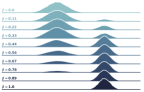
(a) $q=0$

(b) $q=0.5$

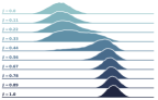
(c) $q=0.9$

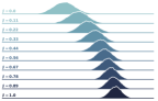
(d) $q=1$

Figure 1: Intermediate densities between $\mathcal{N}(-4,3)$ and $\mathcal{N}(4,1)$ for various $q$-paths and 10 equally spaced $\beta$. The path approaches a mixture of Gaussians with weight $\beta$ at $q=0$. For the geometric mixture ($q=1$), intermediate $\pi_{\beta}$ stay within the exponential family since both $\pi_{0}$, $\pi_{T}$ are Gaussian.

$q$-Exponential Family

The $q$-exponential in Eq. 9 may be used to define a $q$-exponential family of distributions [7, 26]. Using $\theta$ as the natural parameter,

$$\pi_{\theta}^{(q)}(z) =\tilde{\pi}_{0}(z)\,\exp_{q}\big{\{}\theta\cdot\phi_{q}(z)-\psi_{q}(\theta)\big{\}}\,,$$ (11)

which recovers the standard exponential family at $q\to 1$. In App. B.2 we show that the $q$-mixture $\tilde{\pi}^{(\alpha)}_{\beta}$ in Eq. 8 can be rewritten in terms of the $q$-exponential family

$$\pi_{\beta}^{(q)}(z) =\frac{1}{Z^{(q)}_{\beta}}\,\tilde{\pi}_{0}(z)\,\exp_{q}\big{\{}\beta\cdot\ln_{q}\frac{\tilde{\pi}_{T}(z)}{\tilde{\pi}_{0}(z)}\big{\}} Z^{(q)}_{\beta}=\int\tilde{\pi}_{\beta}^{(q)}(z)\,dz$$ (12)

with sufficient statistic $\phi_{q}(z)=\ln_{q}\tilde{\pi}_{T}/\tilde{\pi}_{0}$ and natural parameter $\beta$. The expression in (12) might be used to directly estimate the normalization constant $Z^{(q)}_{\beta}$ via Monte Carlo approximation.

As for the standard exponential family, the $q$-free energy $\psi_{q}(\theta)$ in Eq. 11 is convex in $\theta$ and can be used to construct a Bregman divergence over normalized $q$-exponential family distributions [7]. However, to normalize (12) using the $q$-free energy, a non-linear mapping $\theta(\beta)$ between parameterizations is required. This delicate issue of normalization in the $q$-exponential family has been noted in [22, 30, 26], and we provide more detailed discussion in App. B.3.

Variational Representation using the $\alpha$-Divergence

Since we do not have access to normalization constants in the ais setting, we focus on the $\alpha$-divergence [2, 4] over unnormalized measures $\tilde{q}(z)$ and $\tilde{p}(z)$. We first recall the definition,

$$D_{\alpha}[\tilde{q}(z):\tilde{p}(z)] =\frac{4}{(1-\alpha^{2})}\bigg{(}\frac{1-\alpha}{2}\int\tilde{q}(z)\,dz+\frac{1+\alpha}{2}\int\tilde{p}(z)\,dz-\int\tilde{q}(z)^{\frac{1-\alpha}{2}}\,\tilde{p}(z)^{\frac{1+\alpha}{2}}dz\bigg{)}$$

which is an $f$-divergence [1] for the generator $f(u)=\frac{4}{1-\alpha^{2}}\big{(}\frac{1-\alpha}{2}+\frac{1+\alpha}{2}u-u^{\frac{1+\alpha}{2}}\big{)}$ [4, 5]. Note that $\lim\limits_{\alpha\rightarrow 1}D_{\alpha}[\tilde{q}(z):\tilde{p}(z)]=D_{KL}[\tilde{p}(z):\tilde{q}(z)]$ and $\lim\limits_{\alpha\rightarrow-1}D_{\alpha}[\tilde{q}(z):\tilde{p}(z)]=D_{KL}[\tilde{q}(z):\tilde{p}(z)]$.

In App. C, we follow similar derivations as Amari [3] to show that, for $q=\frac{1+\alpha}{2}$ ([4] Ch. 4), the $q$-path density $\tilde{\pi}^{(q)}_{\beta}$ minimizes the expected $\alpha$-divergence to the endpoints

$$\tilde{\pi}^{(q)}_{\beta}(z) =\operatorname*{arg\,min}\limits_{\tilde{r}(z)}\,(1-\beta)\,D_{\alpha}[\tilde{\pi}_{0}(z):\tilde{r}(z)]+\,\beta\,D_{\alpha}[\tilde{\pi}_{T}(z):\tilde{r}(z)]\,,$$ (13)

where the optimization is over arbitrary $\tilde{r}(z)$. This variational representation generalizes Eq. 5, since the kl divergence is recovered (with the order of the arguments reversed) as $\alpha\rightarrow 1$ or $q\rightarrow 1$.

Moment-Matching Procedures

At $q=0$, the solution to the optimization (13) correponds to the arithmetic mean, or mixture distribution $\tilde{\pi}_{t}^{(0)}(z)=(1-\beta)\,\tilde{\pi}_{0}+\beta\,\tilde{\pi}_{1}$. While the ‘moment-averaged’ ais path [13] appears related to the $q=0$ case, we clarify in App. C.1 that Grosse et al. [13] restrict to optimization within an exponential family of distributions. Generalizing this approach to the $\alpha$-divergence, Bui [10] follows Minka [24] (Sec. 3.1-2) to derive the moment-matching condition

$$\tilde{r}^{*}_{t,\alpha}(z) :=\operatorname*{arg\,min}\limits_{\tilde{r}(z)}(1-\beta)\,D_{\alpha}[\tilde{\pi}_{0}(z):\tilde{r}(z)]+\,\beta\,D_{\alpha}[\tilde{\pi}_{T}(z):\tilde{r}(z)]$$ (14)

$$\implies\mathbb{E}_{\tilde{r}_{*}}[\phi(z)] =(1-\beta)\mathbb{E}_{\tilde{\pi}_{0}^{\alpha}r_{*}^{1-\alpha}}[\phi(z)]+\beta\,\mathbb{E}_{\tilde{\pi}_{T}^{\alpha}\tilde{r}_{*}^{1-\alpha}}[\phi(z)]$$ (15)

where $\tilde{r}(z)$ comes from an exponential family with sufficient statistics $\phi(z)$.

However, we note that our $q$-path is more general than these approaches, since the optimization in Eq. 13 is over all unnormalized distributions. Unlike the moment matching conditions above, our closed form expression for $\tilde{\pi}_{\beta}^{(q)}$ can be directly used as an energy function for mcmc sampling.

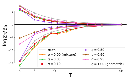
Figure 2: bdmc lower and upper bound estimates of $\log Z_{T}/Z_{0}$ by $q$-path order and number of intermediate distributions ($T$), for annealing between $\mathcal{N}(-4,3)\to\mathcal{N}(4,1)$.

$q$	$Z_{\text{est}}$ ($Z_{\text{true}}=1$)
0.00 (mix)	1.0136 $\pm$ 0.0634
0.05	1.0105 $\pm$ 0.0569
0.10	1.0198 $\pm$ 0.0576
0.90	0.9975 $\pm$ 0.0085
0.95	0.9971 $\pm$ 0.0092
1.00 (geo)	0.9967 $\pm$ 0.0094

Table 1: Partition Function Estimates for various $q$ and linearly spaced ${T=100}$. A path with $q=0.90$ outperforms both the mixture of Gaussians ($q=0$) and geometric ($q=1$) paths in terms of $Z_{\text{err}}=|Z_{\text{est}}-Z_{\text{true}}|$.

4 Experiments

We consider $q$-paths between $\pi_{0}=\mathcal{N}(-4,3)$ and $\pi_{T}=\mathcal{N}(4,1)$ to estimate $Z_{T}/Z_{0}=1$, and use parallel runs of Hamiltonian Monte Carlo (hmc) [28] to obtain accurate, independent samples from $\tilde{\pi}^{(q)}_{t}(z)$ linearly spaced between $\beta_{0}=0$ and $\beta_{T}=1$. For all experiments, we use 10k samples from each intermediate distribution and average results across 20 seeds.

In Fig. 2, we report bdmc upper and lower bound estimates of $\log Z_{T}/Z_{1}$ for various $q$ and $T$. We observe that the choice of $q$ can impact performance, with $q=0.9$ obtaining tighter estimates at small $T$ and $q=0.5$ converging more quickly as $T$ increases. Both outperform the baseline geometric path at $q=1$. In Table 1, we estimate $Z_{T}/Z_{0}$ using ais for $T=100$, and observe that our the $q=0.9$ path can achieve a lower error than the geometric path.

Finally, in App. E, we provide additional analysis for annealing between two Student-$t$ distributions. The Student-$t$ family can be shown to correspond to a $q$-exponential family [21], with the same sufficient statistics as a Gaussian, and a degrees of freedom parameter $\nu$ that induces heavier tails and sets the value of $q$. As $q\rightarrow 1$ or $\nu\rightarrow\infty$, the standard Gaussian is recovered. In Fig. 3-4, we compare annealing between two Student-$t$ distributions in the $q=2$ family to the Gaussian case of $q=1$, and observe that the same $q$-path can induce different qualitative behavior based on properties of the endpoint distributions.

5 Conclusion

In this work, we propose $q$-paths to generalize the geometric mixture path commonly used in ais, and show that modifying the path can improve ais and bdmc for a fixed mixing schedule on a toy Gaussian example. We interpreted our $q$-paths using the deformed logarithm, $q$-exponential family, and $\alpha$-divergences, which may suggest further connections in non-extensive thermodynamics and information geometry. Choosing a schedule for a given $q$-path, understanding how the choice of $q$ depends on properties of the initial and target distributions, and exploring the use of $q$-paths in related methods such as the thermodynamic variational objective (tvo) [20, 9] remain interesting directions for future work.

Appendix A Abstract Mean is Invariant to Affine Transformations

In this section, we show that $h_{q}(u)$ is invariant to affine transformations. That is, for any choice of $a$ and $b$,

$$h_{q}(u)=\begin{cases}a\cdot u^{1-q}+b\hfill&q\neq 1\\ \log u\hfill&q=1\end{cases}$$ (16)

yields the same expression for the abstract mean $\mu_{h_{\alpha}}$. First, we note the expression for the inverse $h^{-1}_{q}(u)$ at $q\neq 1$

$$h^{-1}_{q}(u)=\left(\frac{u-b}{a}\right)^{\frac{1}{1-q}}.$$ (17)

Recalling that $\sum_{i}w_{i}=1$, the abstract mean then becomes

$$\mu_{h_{q}}(\{w_{i}\},\{u_{i}\}) =h_{q}^{-1}\left(\sum_{i}w_{i}h_{q}(u_{i})\right)$$ (18)

$$=h_{q}^{-1}\left(a\left(\sum_{i}w_{i}u_{i}^{1-q}\right)+b\right)$$ (19)

$$=\bigg{(}\sum_{i}w_{i}u_{i}^{1-q}\bigg{)}^{\frac{1}{1-q}}$$ (20)

which is independent of both $a$ and $b$.

Appendix B Derivations of the $q$-Path

B.1 Deformed Log Mixture

In this section, we show that the unnormalized $\ln_{q}$ mixture

$$\ln_{q}\tilde{\pi}^{(q)}_{\beta}(z) =(1-\beta)\ln_{q}\tilde{\pi}_{0}(z)+\beta\ln_{q}\tilde{\pi}_{1}(z)$$ (21)

reduces to the form of the $q$-path intermediate distribution in (2) and (8). Taking $\exp_{q}$ of both sides,

$$\tilde{\pi}^{(q)}_{\beta}(z) =\exp_{q}\left\{(1-\beta)\ln_{q}\tilde{\pi}_{0}(z)+\beta\ln_{q}\tilde{\pi}_{1}(z)\right\}$$

$$=\left[1+(1-q)\left(\ln_{q}\tilde{\pi}_{0}(z)+\beta\left(\ln_{q}\tilde{\pi}_{1}(z)-\ln_{q}\tilde{\pi}_{0}(z)\right)\right)\right]_{+}^{\frac{1}{1-q}}$$

$$=\left[1+(1-q)\frac{1}{1-q}\left(\tilde{\pi}_{0}(z)^{1-q}-1+\beta\big{(}\tilde{\pi}_{1}(z)^{1-q}-1-\tilde{\pi}_{0}(z)^{1-q}+1\big{)}\right)\right]_{+}^{\frac{1}{1-q}}$$

$$=\left[1+\tilde{\pi}_{0}(z)^{1-q}-1+\beta\bigg{(}\tilde{\pi}_{1}(z)^{1-q}-\tilde{\pi}_{0}(z)^{1-q}\bigg{)}\right]_{+}^{\frac{1}{1-q}}$$

$$=\left[\tilde{\pi}_{0}(z)^{1-q}+\beta\,\tilde{\pi}_{1}(z)^{1-q}-\beta\,\tilde{\pi}_{0}(z)^{1-q}\right]_{+}^{\frac{1}{1-q}}$$

$$=\left[(1-\beta)\,\tilde{\pi}_{0}(z)^{1-q}+\beta\,\tilde{\pi}_{1}(z)^{1-q}\,\right]_{+}^{\frac{1}{1-q}}$$

B.2 $q$-Exponential Family

Here, we show that the unnormalized $q$-path reduces to a form of the $q$-exponential family

$$\tilde{\pi}^{(q)}_{\beta}(z) =\bigg{[}(1-\beta)\tilde{\pi}_{0}(z)^{1-q}+\beta\tilde{\pi}_{1}(z)^{1-q}\bigg{]}^{\frac{1}{1-q}}$$ (22)

$$=\bigg{[}\tilde{\pi}_{0}(z)^{1-q}+\beta\big{(}\tilde{\pi}_{1}(z)^{1-q}-\tilde{\pi}_{0}(z)^{1-q}\big{)}\bigg{]}^{\frac{1}{1-q}}$$ (23)

$$=\tilde{\pi}_{0}(z)\left[1+\beta\left(\left(\frac{\tilde{\pi}_{1}(z)}{\tilde{\pi}_{0}(z)}\right)^{1-q}-1\right)\right]^{\frac{1}{1-q}}$$ (24)

$$=\tilde{\pi}_{0}(z)\left[1+(1-q)\,\beta\,\ln_{q}\left(\frac{\tilde{\pi}_{1}(z)}{\tilde{\pi}_{0}(z)}\right)\right]^{\frac{1}{1-q}}$$ (25)

$$=\tilde{\pi}_{0}(z)\exp_{q}\left\{\beta\cdot\ln_{q}\left(\frac{\tilde{\pi}_{1}(z)}{\tilde{\pi}_{0}(z)}\right)\right\}.$$ (26)

Defining $\phi(z)=\ln_{q}\frac{\tilde{\pi}_{1}(z)}{\tilde{\pi}_{0}(z)}$ and introducing a multiplicative normalization factor $Z_{q}(\beta)$, we arrive at

$$\pi^{(q)}_{\beta}(z)=\frac{1}{Z_{q}(\beta)}\,\tilde{\pi}_{0}(z)\exp_{q}\left\{\beta\cdot\phi(z)\right\}\qquad Z_{q}(\beta) :=\int\tilde{\pi}_{0}(z)\exp_{q}\left\{\beta\cdot\phi(z)\right\}\,dz.$$ (27)

B.3 Normalization in q-Exponential Families

The $q$-exponential family can also be written using the $q$-free energy $\psi_{q}(\theta)$ for normalization [7, 26],

$$\pi_{\theta}^{(q)}(z) =\pi_{0}(z)\,\exp_{q}\big{\{}\theta\cdot\phi(z)-\psi_{q}(\theta)\big{\}}\,.$$ (28)

However, since $\exp_{q}\{x+y\}=\exp_{q}\{y\}\cdot\exp_{q}\{\frac{x}{1+(1-q)y}\}$ (see [30] or App. D below) instead of $\exp\{x+y\}=\exp\{x\}\cdot\exp\{y\}$ for the standard exponential, we can not easily move between these ways of writing the $q$-family [22].

Mirroring the derivations of Naudts [26] pg. 108, we can rewrite (28) using the above identity for $\exp_{q}\{x+y\}$, as

$$\pi^{(q)}_{\theta}(z) =\pi_{0}(z)\,\exp_{q}\{\theta\cdot\phi(z)-\psi_{q}(\theta)\}$$ (29)

$$=\pi_{0}(z)\,\exp_{q}\{-\psi_{q}(\theta)\}\exp_{q}\big{\{}\frac{\theta\cdot\phi(z)}{1+(1-q)(-\psi_{q}(\theta))}\big{\}}$$ (30)

Our goal is to express $\pi^{(q)}_{\theta}(z)$ using a normalization constant $Z^{(q)}_{\beta}$ instead of the $q$-free energy $\psi_{q}(\theta)$. While the exponential family allows us to freely move between $\psi(\theta)$ and $\log Z_{\theta}$, we must adjust the natural parameters (from $\theta$ to $\beta$) in the $q$-exponential case. Defining

$$\beta =\frac{\theta}{1+(1-q)(-\psi_{q}(\theta))}$$ (31)

$$Z^{(q)}_{\beta} =\frac{1}{\exp_{q}\{-\psi_{q}(\theta)\}}$$ (32)

we can obtain a new parameterization of the $q$-exponential family, using parameters $\beta$ and multiplicative normalization constant $Z^{(q)}_{\beta}$,

$$\pi^{(q)}_{\beta}(z) =\frac{1}{Z^{(q)}_{\beta}}\pi_{0}(z)\,\exp_{q}\{\beta\cdot\phi(z)\}$$ (33)

$$=\pi_{0}(z)\,\exp_{q}\big{\{}\theta\cdot\phi(z)-\psi_{q}(\theta)\big{\}}=\pi^{(q)}_{\theta}(z)\,.$$ (34)

See Matsuzoe et al. [22], Suyari et al. [30], and Naudts [26] for more detailed discussion of normalization in deformed exponential families.

Appendix C Minimizing $\alpha$-divergences

Amari [3] shows that the $\alpha$ power mean $\pi^{(\alpha)}_{\beta}$ minimizes the expected divergence to a single distribution, for normalized measures and $\alpha=2q-1$. We repeat similar derivations but for the case of unnormalized endpoints $\{\tilde{\pi}_{i}\}$ and $\tilde{r}(z)$

$$\tilde{\pi}_{\alpha}(z) =\operatorname*{arg\,min}\limits_{\tilde{r}(z)}\sum\limits_{i=1}^{N}w_{i}\,D_{\alpha}[\tilde{\pi}_{i}(z):\tilde{r}(z)]$$ (35)

$$\text{where}\quad\tilde{\pi}_{\alpha}(z) =\big{(}\sum\limits_{i=1}^{N}w_{i}\,\tilde{\pi}_{i}(z)^{\frac{1-\alpha}{2}}\big{)}^{\frac{2}{1-\alpha}}$$ (36)

Proof.

$$\frac{d}{d\tilde{r}}\sum\limits_{i=1}^{N}w_{i}\,D_{\alpha}[\tilde{\pi}_{i}(z):\tilde{r}(z)] =\frac{d}{d\tilde{r}}\frac{4}{1-\alpha^{2}}\sum\limits_{i=1}^{N}w_{i}\big{(}-\int\tilde{\pi}_{i}(z)^{\frac{1-\alpha}{2}}\,\tilde{r}(z)^{\frac{1+\alpha}{2}}dz+\frac{1+\alpha}{2}\int\tilde{r}(z)dz\big{)}$$ (37)

$$0 =\frac{4}{1-\alpha^{2}}\big{(}-{\frac{1+\alpha}{2}}\sum\limits_{i=1}^{N}w_{i}\,\tilde{\pi}_{i}(z)^{\frac{1-\alpha}{2}}\,\tilde{r}(z)^{\frac{1+\alpha}{2}-1}+\frac{1+\alpha}{2}\big{)}$$ (38)

$$-\frac{2}{1-\alpha} =-\frac{2}{1-\alpha}\sum\limits_{i=1}^{N}w_{i}\,\tilde{\pi}_{i}(z)^{\frac{1-\alpha}{2}}\tilde{r}(z)^{-\frac{1-\alpha}{2}}$$ (39)

$$\tilde{r}(z)^{\frac{1-\alpha}{2}} =\sum\limits_{i=1}^{N}w_{i}\,\tilde{\pi}_{i}(z)^{\frac{1-\alpha}{2}}$$ (40)

$$\tilde{r}(z) =\bigg{(}\sum\limits_{i=1}^{N}w_{i}\,\tilde{\pi}_{i}(z)^{\frac{1-\alpha}{2}}\bigg{)}^{\frac{2}{1-\alpha}}$$ (41)

∎

This result is similar to a general result about Bregman divergences in Banerjee et al. [8] Prop. 1. although $D_{\alpha}$ is not a Bregman divergence over normalized distributions.

C.1 Arithmetic Mean ($q=0$)

For normalized distributions, we note that the moment-averaging path from Grosse et al. [13] is not a special case of the $\alpha$-integration [3]. While both minimize a convex combination of reverse kl divergences, Grosse et al. [13] minimize within the constrained space of exponential families, while Amari [3] optimizes over all normalized distributions.

More formally, consider minimizing the functional

$$J[r] =(1-\beta)\int\pi_{0}(z)\log\frac{\pi_{0}(z)}{r(z)}dz+\beta\int\pi_{1}(z)\log\frac{\pi_{1}(z)}{r(z)}dz$$ (42)

$$=\text{const}-\int\left[(1-\beta)\pi_{0}(z)+\beta\pi_{1}(z)\right]\log r(z)dz$$ (43)

We will show how Grosse et al. [13] and Amari [3] minimize (43).

Solution within Exponential Family

Grosse et al. [13] constrains $r(z)=\frac{1}{Z(\theta)}h(z)\exp(\theta^{T}g(z))$ to be a (minimal) exponential family model and minimizes (43) w.r.t $r$’s natural parameters $\theta$ (cf. [13] Appendix 2.2):

$$\theta^{*}_{i} =\operatorname*{arg\,min}_{\theta}J(\theta)$$ (44)

$$=\operatorname*{arg\,min}_{\theta}\left(-\int\left[(1-\beta)\pi_{0}(z)+\beta\pi_{1}(z)\right]\left[\log h(z)+\theta^{T}g(z)-\log Z(\theta)\right]dz\right)$$ (45)

$$=\operatorname*{arg\,min}_{\theta}\left(\log Z(\theta)-\int\left[(1-\beta)\pi_{0}(z)+\beta\pi_{1}(z)\right]\theta^{T}g(z)dz+\text{const}\right)$$ (46)

where the last line follows because $\pi_{0}(z)$ and $\pi_{1}(z)$ are assumed to be correctly normalized. Then to arrive at the moment averaging path, we compute the partials $\frac{\partial J(\theta)}{\partial\theta_{i}}$ and set to zero:

$$\frac{\partial J(\theta)}{\partial\theta_{i}} =\operatorname{\mathbb{E}}_{r}[g_{i}(z)]-(1-\beta)\operatorname{\mathbb{E}}_{\pi_{0}}[g_{i}(z)]-\beta\operatorname{\mathbb{E}}_{\pi_{1}}[g_{i}(z)]=0$$ (47)

$$\operatorname{\mathbb{E}}_{r}[g_{i}(z)] =(1-\beta)\operatorname{\mathbb{E}}_{\pi_{0}}[g_{i}(z)]-\beta\operatorname{\mathbb{E}}_{\pi_{1}}[g_{i}(z)]$$ (48)

where we have used the exponential family identity $\frac{\partial\log Z(\theta)}{\partial\theta_{i}}=\operatorname{\mathbb{E}}_{r_{\theta}}[g_{i}(z)]$ in the first line.

General Solution

Instead of optimizing in the space of minimal exponential families, Amari [3] instead adds a Lagrange multiplier to (43) and optimizes $r$ directly (cf. [3] eq. 5.1 - 5.12)

$${r}^{*} =\operatorname*{arg\,min}_{r}J^{\prime}[r]$$ (49)

$$=\operatorname*{arg\,min}_{r}J[r]+\lambda\left(1-\int r(z)dz\right)$$ (50)

Eq. 50 can be minimized using the Euler-Lagrange equations or using the identity

$$\frac{\delta f(x)}{\delta f(x^{\prime})}=\delta(x-x^{\prime})$$ (51)

from [23]. We compute the functional derivative of $J^{\prime}[r]$ using (51) and solve for $r$:

$$\frac{\delta J^{\prime}[r]}{\delta r(z)}= -\int\big{[}(1-\beta)\pi_{0}(z^{\prime})+\beta\pi_{1}(z^{\prime})\big{]}\frac{1}{r(z^{\prime})}\frac{\delta r(z^{\prime})}{\delta r(z)}dz^{\prime}-\lambda\int\frac{\delta r(z^{\prime})}{\delta r(z)}dz^{\prime}$$ (52)

$$= -\int\big{[}(1-\beta)\pi_{0}(z^{\prime})+\beta\pi_{1}(z^{\prime})\big{]}\frac{1}{r(z^{\prime})}\delta(z-z^{\prime})dz^{\prime}-\lambda\int\delta(z-z^{\prime})dz^{\prime}$$ (53)

$$= -\big{[}(1-\beta)\pi_{0}(z)+\beta\pi_{1}(z)\big{]}\frac{1}{r(z)}-\lambda=0$$ (54)

Therefore

$$r(z)\propto\big{[}(1-\beta)\pi_{0}(z)+\beta\pi_{1}(z)\big{]},$$ (55)

which corresponds to our $q$-path at $q=0$, or $\alpha=-1$ in Amari [3]. Thus, while both Amari [3] and Grosse et al. [13] start with the same objective, they arrive at different optimum because they optimize over different spaces.

Appendix D Sum and Product Identities for $q$-Exponentials

In this section, we prove two lemmas which are useful for manipulation expressions involving $q$-exponentials, for example in moving between Eq. 29 and Eq. 30 in either direction.

Lemma 1.

Sum identity

$$\exp_{q}\left(\sum_{n=1}^{N}x_{n}\right)=\prod_{n=1}^{N}\exp_{q}\left(\frac{x_{n}}{1+(1-q)\sum_{i=1}^{n-1}x_{i}}\right)$$ (56)

Lemma 2.

Product identity

$$\prod_{n=1}^{N}\exp_{q}(x_{n})=\exp_{q}\left(\sum_{n=1}^{N}x_{n}\cdot\prod_{i=1}^{n-1}\left(1+(1-q)x_{i}\right)\right)$$ (57)

D.1 Proof of Lemma 1

Proof.

We prove by induction. The base case ($N=1$) is satisfied using the convention $\sum_{i=a}^{b}x_{i}=0$ if $b<a$ so that the denominator on the rhs of Eq. 56 is $1$. Assuming Eq. 56 holds for $N$,

$$\exp_{q}\left(\sum_{n=1}^{N+1}x_{n}\right) =\left[1+(1-q)\sum_{n=1}^{N+1}x_{n}\right]_{+}^{1/(1-q)}$$ (58)

$$=\left[1+(1-q)\left(\sum_{n=1}^{N}x_{n}\right)+(1-q)x_{N+1}\right]_{+}^{1/(1-q)}$$ (59)

$$=\left[\left(1+(1-q)\sum_{n=1}^{N}x_{n}\right)\left(1+(1-q)\frac{x_{N+1}}{1+(1-q)\sum_{n=1}^{N}x_{n}}\right)\right]_{+}^{1/(1-q)}$$ (60)

$$=\exp_{q}\left(\sum_{n=1}^{N}x_{n}\right)\exp_{q}\left(\frac{x_{N+1}}{1+(1-q)\sum_{n=1}^{N}x_{n}}\right)$$ (61)

$$=\prod_{n=1}^{N+1}\exp_{q}\left(\frac{x_{n}}{1+(1-q)\sum_{i=1}^{n-1}x_{i}}\right)\text{(using the inductive hypothesis)}$$ (62)

∎

D.2 Proof of Lemma 2

Proof.

We prove by induction. The base case ($N=1$) is satisfied using the convention $\prod_{i=a}^{b}x_{i}=1$ if $b<a$. Assuming Eq. 57 holds for $N$, we will show the $N+1$ case. To simplify notation we define $y_{N}:=\sum_{n=1}^{N}x_{n}\cdot\prod_{i=1}^{n-1}\left(1+=(1-q)x_{i}\right)$. Then,

$$\prod_{n=1}^{N+1}\exp_{q}(x_{n}) =\exp_{q}(x_{1})\left(\prod_{n=2}^{N+1}\exp_{q}(x_{n})\right)$$ (63)

$$=\exp_{q}(x_{0})\left(\prod_{n=1}^{N}\exp_{q}(x_{n})\right) n\to n-1)$$ (reindex

$$=\exp_{q}(x_{0})\exp_{q}(y_{N})$$ (inductive hypothesis)

$$=\bigg{[}\left(1+(1-q)\cdot x_{0}\right)\left(1+(1-q)\cdot y_{N}\right)\bigg{]}_{+}^{1/(1-q)}$$ (64)

$$=\bigg{[}1+(1-q)\cdot x_{0}+\big{(}1+(1-q)\cdot x_{0}\big{)}(1-q)\cdot y_{N}\bigg{]}_{+}^{1/(1-q)}$$ (65)

$$=\bigg{[}1+(1-q)\bigg{(}x_{0}+\big{(}1+(1-q)\cdot x_{0}\big{)}y_{N}\bigg{)}\bigg{]}_{+}^{1/(1-q)}$$ (66)

$$=\exp_{q}\left(x_{0}+\big{(}1+(1-q)\cdot x_{0}\big{)}y_{N}\right)$$ (67)

Next we use the definition of $y_{N}$ and rearrange

$$=\exp_{q}\left(x_{0}+\big{(}1+(1-q)\cdot x_{0}\big{)}\left(x_{1}+x_{2}(1+(1-q)\cdot x_{1})+...+x_{N}\cdot\prod_{i=1}^{N-1}(1+(1-q)\cdot x_{i})\right)\right)$$

$$=\exp_{q}\left(\sum_{n=0}^{N}x_{n}\cdot\prod_{i=1}^{n-1}\left(1+(1-q)x_{i}\right)\right).$$ (68)

Then reindexing $n\to n+1$ establishes

$$\prod_{n=1}^{N+1}\exp_{q}(x_{n})=\exp_{q}\left(\sum_{n=1}^{N+1}x_{n}\cdot\prod_{i=1}^{n-1}\left(1+(1-q)x_{i}\right)\right).$$ (69)

∎

Appendix E Annealing between Student-$t$ Distributions

E.1 Student-$t$ Distributions and $q$-Exponential Family

The Student-$t$ distribution appears in hypothesis testing with finite samples, under the assumption that the sample mean follows a Gaussian distribution. In particular, the degrees of freedom parameter $\nu=n-1$ can be shown to correspond to an order of the ${q}$-exponential family with $\nu=(3-{q})/({q}-1)$ (in 1-d), so that the choice of ${q}$ is linked to the amount of data observed.

We can first write the multivariate Student-$t$ density, specified by a mean vector $\mu$, covariance ${\mathbf{\Sigma}}$, and degrees of freedom parameter $\nu$, in $d$ dimensions, as

$$t_{\nu}(x|{\mathbf{\mu}},{\mathbf{\Sigma}})=\frac{1}{Z(\nu,{\mathbf{\Sigma}})}\big{[}1+\frac{1}{\nu}(x-{\mathbf{\mu}})^{T}{\mathbf{\Sigma}}^{-1}(x-{\mathbf{\mu}})\big{]}^{-\big{(}\frac{\nu+d}{2}\big{)}}$$ (70)

where $Z(\nu,{\mathbf{\Sigma}})=\Gamma(\frac{\nu+d}{2})/\Gamma(\frac{\nu}{2})\cdot|{\mathbf{\Sigma}}|^{-1/2}\nu^{-\frac{d}{2}}\pi^{-\frac{d}{2}}$. Note that $\nu>0$, so that we only have positive values raised to the $-(\nu+d)/2$ power, and the density is defined on the real line.

The power function in (70) is already reminiscent of the ${q}$-exponential, while we have first and second moment sufficient statistics as in the Gaussian case. We can solve for the exponent, or order parameter $q$, that corresponds to $-(\nu+d)/2$ using $-\big{(}\frac{\nu+d}{2}\big{)}=\frac{1}{1-{q}}$. This results in the relations

$$\nu=\frac{d-d{q}+2}{{q}-1}\qquad\text{or}\qquad{q}=\frac{\nu+d+2}{\nu+d}$$ (71)

We can also rewrite the $\nu^{-1}\,(x-{\mathbf{\mu}})^{T}{\mathbf{\Sigma}}^{-1}(x-{\mathbf{\mu}})$ using natural parameters corresponding to $\{x,x^{2}\}$ sufficient statistics as in the Gaussian case (see, e.g. Matsuzoe and Wada [21] Example 4).

Note that the Student-$t$ distribution has heavier tails than a standard Gaussian, and reduces to a multivariate Gaussian as ${q}\rightarrow 1$ and $\exp_{{q}}(u)\rightarrow\exp(u)$. This corresponds to observing $n\rightarrow\infty$ samples, so that the sample mean and variance approach the ground truth [25].

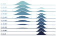
(a) $q=0$

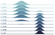
(b) $q=0.5$

(c) $q=0.9$

(d) $q=1$

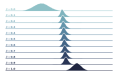
(e) $q=2$

Figure 3: Intermediate densities between $\mathcal{N}(-4,3)$ and $\mathcal{N}(4,1)$ for various $q$-paths and 10 equally spaced $\beta$. The path approaches a mixture of Gaussians with weight $\beta$ at $q=0$. For the geometric mixture ($q=1$), intermediate $\pi_{\beta}$ stay within the exponential family since both $\pi_{0}$, $\pi_{T}$ are Gaussian.

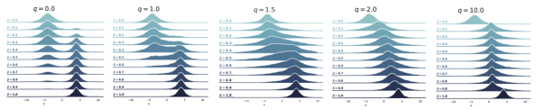
Figure 4: Intermediate densities between Student-$t$ distributions, $t_{\nu=1}(-4,3)$ and $t_{\nu=1}(4,1)$ for various $q$-paths and 10 equally spaced $\beta$, Note that $\nu=1$ corresponds to $q=2$, so that the $q=2$ path stays within the $q$-exponential family.
We provide code to reproduce experiments at https://github.com/vmasrani/q_paths.

E.2 Annealing between 1-d Student-$t$ Distributions

Since the Student-$t$ family generalizes the Gaussian distribution to $q\neq 1$, we can run a similar experiment annealing between two Student-$t$ distributions. We set $q=2$, which corresponds to $\nu=1$ with $\nu=(3-{q})/({q}-1)$, and use the same mean and variance as the Gaussian example in Fig. 3, with $\pi_{0}(z)=t_{\nu=1}(-4,3)$ and $\pi_{1}(z)=t_{\nu=1}(4,1)$.

We visualize the results in Fig. 4. For this special case of both endpoint distributions within a parametric family, we can ensure that the $q=2$ path stays within the $q$-exponential family of Student-$t$ distributions. We make a similar observation for the Gaussian case and $q=1$ in Fig. 3. Comparing the $q=0.5$ and $q=0.9$ Gaussian path with the $q=1.0$ and $q=1.5$ path, we observe that mixing behavior appears to depend on the relation between the $q$-path parameter and the order of the $q$-exponential family of the endpoints.

As $q\rightarrow\infty$, the power mean (6) approaches the $\min$ operation as $1-q\rightarrow-\infty$. In the Gaussian case, we see that, even at $q=2$, intermediate densities for all $\beta$ appear to concentrate in regions of low density under both $\pi_{0}$ and $\pi_{T}$. However, for the heavier-tailed Student-$t$ distributions, we must raise the $q$-path parameter significantly to observe similar behavior.

E.3 Endpoints within a Parametric Family

If the two endpoints $\tilde{\pi}_{0},\tilde{\pi}_{T}$ are within a $q$-exponential family, we can show that each intermediate distribution along the $q$-path of the same order is also within this $q$-family. However, we cannot make such statements for general endpoint distributions or members of different $q$-exponential families.

Exponential Family Case

We assume potentially vector valued parameters $\theta=\{\theta\}_{i=1}^{N}$ with multiple sufficient statistics $\phi(z)=\{\phi_{i}(z)\}_{i=1}^{N}$, with $\theta\cdot\phi(z)=\sum_{i=1}^{N}\theta_{i}\phi_{i}(z)$. For a common base measure $g(z)$, let $\tilde{\pi}_{0}(z)=g(z)\,\exp\{\theta_{0}\cdot\phi(z)\}$ and $\tilde{\pi}_{1}(z)=g(z)\,\exp\{\theta_{1}\cdot\phi(z)\}$. Taking the geometric mixture,

$$\tilde{\pi}_{\beta}(z) =\exp\big{\{}(1-\beta)\,\log\tilde{\pi}_{0}(z)+\beta\,\log\tilde{\pi}_{T}(z)\big{\}}$$ (72)

$$=\exp\big{\{}\log g(z)+(1-\beta)\,\theta_{0}\cdot\phi(z)+\beta\,\theta_{1}\phi(z)\big{\}}$$ (73)

$$=g(z)\exp\big{\{}\big{(}(1-\beta)\,\theta_{0}+\beta\,\theta_{1}\big{)}\cdot\phi(z)\big{\}}$$ (74)

which, after normalization, will be a member of the exponential family with natural parameter $(1-\beta)\,\theta_{0}+\beta\,\theta_{1}$.

$q$-Exponential Family Case

For a common base measure $g(z)$, let $\tilde{\pi}_{0}(z)=g(z)\,\exp_{q}\{\theta_{0}\cdot\phi(z)\}$ and $\tilde{\pi}_{1}(z)=g(z)\,\exp_{q}\{\theta_{1}\cdot\phi(z)\}$. The $q$-path intermediate density becomes

$$\tilde{\pi}^{(q)}_{\beta}(z) =\big{[}(1-\beta)\,\tilde{\pi}_{0}(z)^{1-q}+\beta\,\tilde{\pi}_{T}(z)^{1-q}\big{]}^{\frac{1}{1-q}}$$ (75)

$$=\big{[}(1-\beta)\,g(z)^{1-q}\,\exp_{q}\{\theta_{0}\cdot\phi(z)\}^{1-q}+\beta\,g(z)^{1-q}\,\exp_{q}\{\theta_{1}\cdot\phi(z)\}^{1-q}\big{]}^{\frac{1}{1-q}}$$ (76)

$$=\bigg{[}g(z)^{1-q}\bigg{(}(1-\beta)\,\,[1+(1-q)(\theta_{0}\cdot\phi(z))]^{\frac{1}{1-q}1-q}+\beta\,[1+(1-q)(\theta_{1}\cdot\phi(z))]^{\frac{1}{1-q}1-q}\bigg{)}\bigg{]}^{\frac{1}{1-q}}$$

$$=g(z)\bigg{[}1+(1-q)\bigg{(}\big{(}(1-\beta)\,\theta_{0}+\beta\,\theta_{1}\big{)}\cdot\phi(z)\bigg{)}\bigg{]}^{\frac{1}{1-q}}$$ (77)

$$=g(z)\exp_{q}\big{\{}\big{(}(1-\beta)\,\theta_{0}+\beta\,\theta_{1}\big{)}\cdot\phi(z)\big{\}}$$ (78)

which has the form of an unnormalized $q$-exponential family density with parameter $(1-\beta)\,\theta_{0}+\beta\,\theta_{1}$.

References

Ali and Silvey [1966]
Syed Mumtaz Ali and Samuel D Silvey.
A general class of coefficients of divergence of one distribution
from another.
Journal of the Royal Statistical Society: Series B
(Methodological), 28(1):131–142, 1966.
Amari [1982]
Shun-ichi Amari.
Differential geometry of curved exponential families-curvatures and
information loss.
The Annals of Statistics, pages 357–385, 1982.
Amari [2007]
Shun-ichi Amari.
Integration of stochastic models by minimizing -divergence.
Neural computation, 19(10):2780–2796,
2007.
Amari [2016]
Shun-ichi Amari.
Information geometry and its applications, volume 194.
Springer, 2016.
Amari and Cichocki [2010]
Shun-ichi Amari and Andrzej Cichocki.
Information geometry of divergence functions.
Bulletin of the polish academy of sciences. Technical
sciences, 58(1):183–195, 2010.
Amari and Nagaoka [2007]
Shun-ichi Amari and Hiroshi Nagaoka.
Methods of information geometry, volume 191.
American Mathematical Soc., 2007.
Amari and Ohara [2011]
Shun-ichi Amari and Atsumi Ohara.
Geometry of q-exponential family of probability distributions.
Entropy, 13(6):1170–1185, 2011.
Banerjee et al. [2005]
Arindam Banerjee, Srujana Merugu, Inderjit S Dhillon, and Joydeep Ghosh.
Clustering with Bregman Divergences.
Journal of Machine Learning Research, 6:1705–1749,
2005.
Brekelmans et al. [2020]
Rob Brekelmans, Vaden Masrani, Frank Wood, Greg Ver Steeg, and Aram Galstyan.
All in the exponential family: Bregman duality in thermodynamic
variational inference.
In International Conference on Machine Learning, 2020.
de Carvalho [2016]
Miguel de Carvalho.
Mean, what do you mean?
The American Statistician, 70(3):270–274,
2016.
Gelman and Meng [1998]
Andrew Gelman and Xiao-Li Meng.
Simulating normalizing constants: From importance sampling to bridge
sampling to path sampling.
Statistical science, pages 163–185, 1998.
Grosse et al. [2013]
Roger B Grosse, Chris J Maddison, and Ruslan R Salakhutdinov.
Annealing between distributions by averaging moments.
In Advances in Neural Information Processing Systems, pages
2769–2777, 2013.
Grosse et al. [2015]
Roger B Grosse, Zoubin Ghahramani, and Ryan P Adams.
Sandwiching the marginal likelihood using bidirectional Monte
Carlo.
arXiv preprint arXiv:1511.02543, 2015.
Grosse et al. [2016]
Roger B Grosse, Siddharth Ancha, and Daniel M Roy.
Measuring the reliability of MCMC inference with bidirectional
Monte Carlo.
In Advances in Neural Information Processing Systems, pages
2451–2459, 2016.
Grünwald [2007]
Peter D Grünwald.
The minimum description length principle.
MIT press, 2007.
Hardy et al. [1953]
G.H. Hardy, J.E. Littlewood, and G. Pólya.
Inequalities.
The Mathematical Gazette, 37(321):236–236, 1953.
doi: 10.1017/S0025557200027455.
Jarzynski [1997]
Christopher Jarzynski.
Equilibrium free-energy differences from nonequilibrium measurements:
A master-equation approach.
Physical Review E, 56(5):5018, 1997.
Kolmogorov [1930]
Andrey Kolmogorov.
On the notion of mean.
Mathematics and Mechanics, 1930.
Masrani et al. [2019]
Vaden Masrani, Tuan Anh Le, and Frank Wood.
The thermodynamic variational objective.
Advances in Neural Information Processing Systems, 2019.
Matsuzoe and Wada [2015]
Hiroshi Matsuzoe and Tatsuaki Wada.
Deformed algebras and generalizations of independence on deformed
exponential families.
Entropy, 17(8):5729–5751, 2015.
Matsuzoe et al. [2019]
Hiroshi Matsuzoe, Antonio M Scarfone, and Tatsuaki Wada.
Normalization problems for deformed exponential families.
In International Conference on Geometric Science of
Information, pages 279–287. Springer, 2019.
Meng [2004]
Anders Meng.
An introduction to variational calculus in machine learning.
2004.
Minka [2005]
Tom Minka.
Divergence measures and message passing.
Technical report, Microsoft Research, 2005.
Murphy [2007]
Kevin P Murphy.
Conjugate bayesian analysis of the gaussian distribution.
def, 1(22):16, 2007.
Naudts [2011]
Jan Naudts.
Generalised thermostatistics.
Springer Science & Business Media, 2011.
Neal [2001]
Radford M Neal.
Annealed importance sampling.
Statistics and computing, 11(2):125–139,
2001.
Neal [2011]
Radford M Neal.
MCMC using Hamiltonian dynamics.
Handbook of Markov Chain Monte Carlo, page 113, 2011.
Nielsen [2020]
Frank Nielsen.
An elementary introduction to information geometry.
Entropy, 22(10), 2020.
Suyari et al. [2020]
Hiroki Suyari, Hiroshi Matsuzoe, and Antonio M Scarfone.
Advantages of q-logarithm representation over q-exponential
representation from the sense of scale and shift on nonlinear systems.
The European Physical Journal Special Topics, 229(5):773–785, 2020.
Tsallis [1988]
Constantino Tsallis.
Possible generalization of Boltzmann-Gibbs statistics.
Journal of statistical physics, 52(1-2):479–487, 1988.
Tsallis [2009]
Constantino Tsallis.
Introduction to nonextensive statistical mechanics: approaching
a complex world.
Springer Science & Business Media, 2009.