NAPA: Neural Art Human Pose Amplifier

Abstract

This is the project report for CSCI-GA.2271-001. We target human pose estimation in artistic images. For this goal, we design an end-to-end system that uses neural style transfer for pose regression. We collect a 277-style set for arbitrary style transfer and build an artistic 281-image test set. We directly run pose regression on the test set and show promising results. For pose regression, we propose a 2d-induced bone map from which pose is lifted. To help such a lifting, we additionally annotate the pseudo 3d labels of the full in-the-wild MPII dataset. Further, we append another style transfer as self supervision to improve 2d. We perform extensive ablation studies to analyze the introduced features. We also compare end-to-end with per-style training and allude to the tradeoff between style transfer and pose regression. Lastly, we generalize our model to the real-world human dataset and show its potentiality as a generic pose model. We explain the theoretical foundation in Appendix. We release code at https://github.com/strawberryfg/NAPA-NST-HPE,  data, and  video.

1 Introduction

The aim of human pose estimation is to locate pre-defined keypoints of human figures. Prior work has focused on real-world datasets. There is limited work addressing 3d pose estimation in artistic images.

Neural style transfer can effectively transfer the style of phenomenal artworks onto real images. However, to emulate the different aesthetic effects of artworks paintings, sculptures, existing style sets are not enough. Regarding our application, we build a style set covering different styles and enforce novel style transfer losses. We then empower our pose system with style transfer and attach an auxiliary style transfer in the end to further improve 2d keypoints.

To enable fine pose regression, we decouple the problem into 2d and depth using bone maps. To facilitate the learning of depth therein, we annotate pseudo 3d labels of MPII.

We are the first to showcase high-quality 2d/3d pose predictions on artwork about human figures.

We make additional contributions:

• We investigate end-to-end $vs$ per-style training and compare stylization results. We identify the importance of instance normalization. We display more impressive stylized images using the per-style training strategy and establish a solid baseline.

• We show that our method can be extended to generic pose estimation regardless of genuineness.

• We perform comprehensive ablation studies to expound on all of the introduced features/components.

• We provide theoretical analysis in Appendix.

2 Related Works

Style Transfer [7] introduced neural style transfer by applying convolutional neural nets to reproduce famous painting styles on natural images. The algorithm combined the content of a natural image with the style of a famous painting by minimizing both the feature and style reconstruction losses. The algorithm produced high-quality images, but was computationally expensive as it required both forward and backward passes through a pre-trained network. [12] developed a feed-forward method of neural style transfer that is much faster than the method introduced by [7] with similar qualitative results. Our method for style transfer in this paper is based on [12].

Human Pose Estimation Early works established mathematical models exponential maps [3], shape context[22], Pfinder [29], deformable part models[5], . Deep learning has completely revolutionized this field[16][15][9][23], we refer to [4] for an up-to-date survey. [11] used pose in art composition for image retrieval. [19] analyzed artwork compositions via pose. The closest to our work is a very recent work [20] that used style transfer for pose estimation/image retrieval in Greek vase paintings.

3 Approach

We sketch the overall pipeline in Fig.  1. It consists of three parts: the neural style transfer part (green in Fig.  1), the pose regression part (red), and the self supervision part (blue). During training, the original image containing a person $\mathbf{I}$ is presented to the image transformation network $\mathcal{F}$, which then produces a style transferred image $\mathbf{O}$. The following pose regression network $\mathcal{G}$ takes only the stylized image $\mathbf{O}$ as input and regresses the 3d keypoints $\mathbf{Y}$. Note this is the final output we want: the 3d pose prediction. The extra self supervision part reuses the concept of neural style transfer and tries to reconstruct the stylization $\mathbf{O}$ from the style image $\mathbf{S}$ and the bone map $\mathbf{P}$ (which is derived from 2d keypoints $\mathbf{Y}_{2d}$). The test stage merely maps $\mathbf{I}$ to 3d pose $\mathbf{Y}$ using $\mathbf{G}$. The notation overview is in Appendix Sec. A.

Style Transfer This process stylizes the content image to emulate the artistic effect of the style target. For this stylization, we use the same image transform net $\mathcal{F}$ as [12]. Regarding the style image $\mathbf{S}$, we randomly select from a pool we collected (Sec.  3.1) instead of training one model per style as in [12]. We also tried the approach in [12] and detail the differences between style-specific training and arbitrary style training below in Sec.  4.4.1. Following [12] we utilize a VGG as the loss network and enforce more losses to guide the style transfer process. (Sec.  3.2,  4.4.2).

Pose Regression After transferring, we would like to generate the 3d pose (also called 3d keypoints) $\mathbf{Y}\in\mathbb{R}^{\mathit{J}\times 3}$ ($\mathit{J}=18$) of that human figure. The problem is decoupled into estimating 2d and lifting 2d to 3d. We extract 2d keypoints $\mathbf{Y}_{2d}$ from $\mathcal{G}$: [25] here. Similar to [28] , we visualize the 2d in a kinematic bone map $\mathbf{P}$ and forward it to another depth estimation network $\mathcal{G}^{\prime}$: (a simple Res50 with 1 FC regression head) to obtain depth $\mathbf{Y}_{depth}$. Now we can piece together $\mathbf{Y}_{2d}$ with $\mathbf{Y}_{depth}$ to construct the 3d pose $\mathbf{Y}$. We empirically find this decoupling and the proposed bone map benefit test cases which would otherwise cause bizarre results. (Fig.  10, Sec.  4.4.4) Losses are in Sec.  3.2 .

The bone map rendering function $\mathcal{R}$ runs as follows: For each bone in the kinematics chain [30] connecting $2$ adjacent keypoints $(x_{1},y_{1})$ and $(x_{2},y_{2})$, we define the related area in the bone map as the oval (and its interior) that has $\overrightarrow{(x_{2},y_{2})-(x_{1},y_{1})}$ as the minor axis $\vec{y}$, the major axis $\vec{x}\perp\vec{y}$ and bone width $d$ as the length of the major axis. $d$ effectively controls how wide we want the bone to span. The oval contains a set of loops $[\alpha]$: $\{\hat{\alpha_{i}}:[0,1]\rightarrow\mathit{R}^{2}\mid\hat{\alpha_{i}}\ is\ the\ oval\ \frac{(dist((x,y),\vec{y}))^{2}}{a_{i}^{2}}+\frac{(dist((x,y),\vec{x}))^{2}}{(\frac{dist((x_{1},y_{1}),(x_{2},y_{2}))}{2})^{2}}=1,\ for\ 0\leq a_{1}<a_{2}<...<a_{i}<...<a_{n}=\frac{d}{2}\}$ A more formalized representation of the time-parameterized mapping between $[0,1]$ to the bone map space $\mathcal{P}$ is detailed in Appendix Sec. K. The bone map is finalized simply by colorizing each bone area illustrated above in a 3-channel RGB. The rendering can be better understood from the angle of loops in fundamental groups. (Appendix Sec. I.2)

Self Supervision The appended self supervision loss network corrects the predicted 2d pose by projecting it to the stylization space $\mathcal{O}$ and measuring the difference between the reconstruction $\mathbf{O}^{\prime}\in\mathcal{O}$ and the stylized image $\mathbf{O}\in\mathcal{O}$. We adopt another image transform net $\mathcal{F}^{\prime}$, which is initialized to $\mathcal{F}$, to reconstruct the stylization given the bone map $\mathbf{P}$ above and the style target $\mathbf{S}$. Essentially it can be interpreted as another style transfer on the rendered bone map. We explain more details and the reason why we do not reconstruct the original image in Appendix. Sec. I.

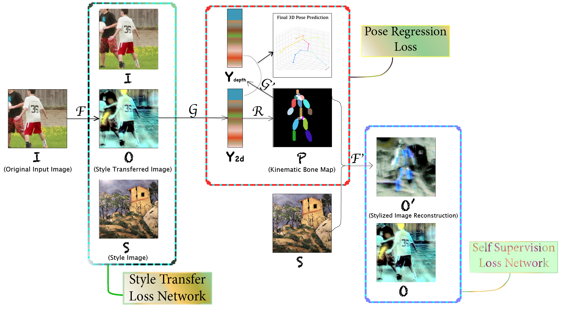
Figure 1: Diagram of the pipeline. During training, the neural style transfer (green) part stylizes the human image and sends the stylization to the pose regression part (red), which outputs the final 3d pose prediction as desired. The self supervision part (blue) aims to improve only the 2d keypoints and can be treated as additional supervision. During testing, the original art image is directly sent to the pose regression part which predicts the 3d pose. The style transfer and self supervision parts are completely discarded.

3.1 Artistic Styles

Our pipeline supports arbitrary style transfer, which is crucial for separating pose from nuisances. Previous style transfer works only have a few most recognized paintings from most well-known painters , which is limited. We build a style dataset of $277$ images covering different styles , which we collect from museums, galleries and books . We use styles ranging from Impressionism, Cubism, Fauvism, to Romanesque, Futurism, Surrealism, Expressionism, Kinetic Art . Some examples are in Appendix Sec. C. We also show some failure cases under this page.

3.2 Losses

Neural Style Transfer Loss

• $\mathcal{L}_{style}(\mathrm{O},\mathrm{S})$: It is the squared Frobenius norm of the difference between the Gram matrices of the style transferred image and the style image [12].

• $\mathcal{L}_{feat}(\mathrm{O},\mathrm{I})$: The feature reconstruction loss between content and stylized image in [12].

• $\mathcal{L}_{tv}(\mathrm{O})$: Total variation loss as in [12].

Note the above are used in the perceptual loss [12] paper.

Besides, we propose the following:

• $\mathcal{L}_{sent}(\mathrm{O},\mathrm{S})$: Jensen Shannon entropy loss between features from stylized image $\mathrm{O}$ and style image $\mathrm{S}$ at layers $\mathbf{relu1\_1}$, $\mathbf{relu1\_2}$ and $\mathbf{relu2\_1}$.

• $\mathcal{L}_{srgb}(\mathrm{O_{srgb}},\mathrm{S_{srgb}})$: Let $\mathrm{O_{srgb}},\mathrm{S_{srgb}}$ be the srgb format of transferred image and style image respectively, the loss is the cosine similarity of these two vectors $\mathrm{O_{srgb}}$ and $\mathrm{S_{srgb}}$. Note losses on other color spaces [8] might further help, we leave that for future work.

• $\mathcal{L}_{hsv}(\mathrm{O},\mathrm{S})$: This is the HSV loss between style transferred image $\mathrm{O}$ and style image $\mathrm{S}$. Let the hue, saturation and vibrance of style image be $\mathrm{h_{s}},\mathrm{s_{s}},\mathrm{v_{s}}$ and the counterparts of the transferred image be $\mathrm{h_{o}},\mathrm{s_{o}},\mathrm{v_{o}}$. $\mathcal{L}_{hsv}=||\mathrm{h_{s}}-\mathrm{h_{o}}||_{1}+||\mathrm{s_{s}}-\mathrm{s_{o}}||_{1}+||\mathrm{v_{s}}-\mathrm{v_{o}}||_{1}$.

• $\mathcal{L}_{cos}(\mathrm{O},\mathrm{S})$: Defined as the cosine similarity between features from style image $\mathrm{S}$ and transferred image $\mathrm{O}$ at layer $\mathbf{relu4\_2}$.

• $\mathcal{L}_{content}(\mathrm{O},\mathrm{I})$: The L2 loss between features from content image $\mathrm{I}$ and stylized image $\mathrm{O}$ at layer $\mathbf{relu4\_2}$.

• $\mathcal{L}_{cent}(\mathrm{O},\mathrm{I})$: Written as the Jensen Shannon entropy loss between features from content image and stylized image at layers $\mathbf{relu5\_2}$, $\mathbf{relu5\_3}$, $\mathbf{relu5\_4}$

To summarize, $\mathcal{L}_{sent}$, $\mathcal{L}_{srgb}$, $\mathcal{L}_{hsv}$ and $\mathcal{L}_{cos}$ relate to style reconstruction loss while $\mathcal{L}_{content}$ and $\mathcal{L}_{cent}$ represent the content reconstruction loss. Practically we observe that among the additional losses apart from those in [12], the following are the most important: $\mathcal{L}_{hsv}$, $\mathcal{L}_{cos}$ and $\mathcal{L}_{srgb}$. We will see this afterwards in Sec.  4.4.2.

Pose Regression Loss As said earlier, we subscribe to the view that lifting from 2d to 3d is better than directly regressing 3d when a generic pose model is required (Sec.  4.5), and so the losses are on 2d and depth respectively.

$\mathcal{L}_{2d}$: Integral loss guides the learning of $\mathcal{G}$ and 2d keypoints prediction $\mathbf{Y}_{2d}$(Fig.  1). It was first put forth in [25].

$\mathcal{L}_{depth}$: We use the orientation representation[18][24][27] and define an euclidean loss between predicted bone vector and ground truth bone vector. This loss forces the model to implicitly learn the depth of keypoints $\mathbf{Y}_{depth}$ by transforming bone vector to joint location. Bone vector is standardized (using mean and std) to facilitate the learning.

Self Supervision Loss The self supervision is a small ”gadget” to refine the 2d by comparing the induced bone map and the stylized image in the stylization space. To initiate the comparison, we adapt the ones in neural style transfer loss above and define the counterparts:

• $\mathcal{L}_{style\_sup}(\mathrm{O^{\prime}},\mathrm{O})$: Similar to $\mathcal{L}_{style}$ except that the difference is between the stylized image: $\mathrm{O}$ and the reconstruction of the stylized image: $\mathrm{O^{\prime}}$.

• $\mathcal{L}_{cos\_sup}(\mathrm{O^{\prime}},\mathrm{O})$: The cosine similarity between $\mathrm{O}$ and its reconstruction $\mathrm{O^{\prime}}$. It is similar to $\mathcal{L}_{cos}$.

• $\mathcal{L}_{feat\_sup}(\mathrm{O^{\prime}},\mathrm{O})$: Now the feature to be reconstructed is $\mathrm{O}$. It is defined at the content layer $\mathbf{relu4\_2}$.

Ratios The learning is all about balancing, most importantly the balancing between the neural style transfer and the pose regression. This is critical for the end-to-end training mechanism in our pipeline, which is not needed for a separate training alternative (Sec.  4.4.1). We empirically set the ratios during training. See Appendix Sec. B.

3.3 Training

The entire pipeline includes a lot of prevalent network architectures. Direct end-to-end training from scratch does not work as there is a slew of losses to balance. In our exploration, we follow a 4-stage training protocol:

stage 1 only learns the style transfer network $\mathcal{F}$ with VGG loss network tunable.

stage 2 only targets at regressing the pose. We warm up the $\mathcal{G}$(2d) with [25], and $\mathcal{G^{\prime}}$(depth) with ResNet50. Images are stylized using weights learned from stage 1.

stage 3 fixes the VGG weight and jointly trains style transfer ($\mathcal{F}$) and pose regression ($\mathcal{G}$ & $\mathcal{G^{\prime}}$).

stage 4 adds self supervision loss training. Another style transfer network $\mathcal{F^{\prime}}$ and another VGG are trained.

We use Human3.6M[10], MPII[2] in training, same as [24][25]. Concerning the pose regression part, we additionally annotate the pseudo 3d ground truth of the entire MPII by manually revising the model-optimized 3d while preserving projection & certain anthropometric constraints joint angle limits[1]. This way, the information of various athletic 3d poses in MPII is retained and best utilized, which is underexplored in prior works. (Sec. 4.4.3, Appendix Sec. E) About the self supervision, we also make use of the vast amount of human images in COCO [17](train2017/val2017). All images are resized to $224\times 224$. No data augmentation is enabled. Training is mostly done on an 8GB GTX 1070 or an 8GB RTX 2080 with batch size = $2$, $3$ or $22$ depending on the stage. Learning rate is initially $0.0001$, which is then decreased upon loss plateau or increment of the stage. We opt for RMSProp with a weight decay of $0.00001$ and momentum set to $0.9$.

4 Experiments

Evaluation Dataset We create a dataset of $281$ images that contains artistic style human figures, most of which come from  Museum of Modern Art,  steampunk: the beginning, Gothic Art and Masterpieces of Impressionism and Post Impressionism: The Annenberg Collection. We develop an annotation tool to annotate the 2d labels. Following the standard, we report results using the PCKh metric that measures the percentage of joints for which the prediction is within a certain threshold to the ground truth. The threshold is set to 25% of the head size throughout the paper. Note this is a strict threshold that requires high-precision estimation. Regarding the 3d pose, since it’s infeasible to obtain it without wearable IMUs or marker-based MoCap systems, we only depict qualitative visualization.

4.1 Baseline

We perform per-style training using the style transfer network and methodology from [12] as a baseline for our neural style transfer to compare against the end-to-end training. For the per-style training, we used the MPII dataset. The images are cropped to focus on the human figures and then resized to $256\times 256$. Training was done on K80 Tesla with a batch size of 4. We used Adam as the optimizer with a learning rate of 0.001. We train a style transfer network for each style and then the MPII dataset is fed through the trained network to generate a style transferred MPII dataset. This style transferred dataset is then used to train a pose regression model for the specific style. We will discuss the differences between the results from the per-style training and end-to-end training in Sec.  4.4.1.

4.1.1 Instance Normalization

The image transformation net from [12] that we used has batch normalization layers after the residual convolution layers. Instance normalization has been shown to generate better qualitative images for fast style transfer than batch normalization with improved convergence speeds. [26] Instance normalization differs from batch normalization in that every image is normalized separately in contrast to in a batch for batch normalization. As we can see from Fig.  2, instance normalization provides for better style transfer than batch normalization as the batch normalization image is mostly the same color and has artifacts around the edges.

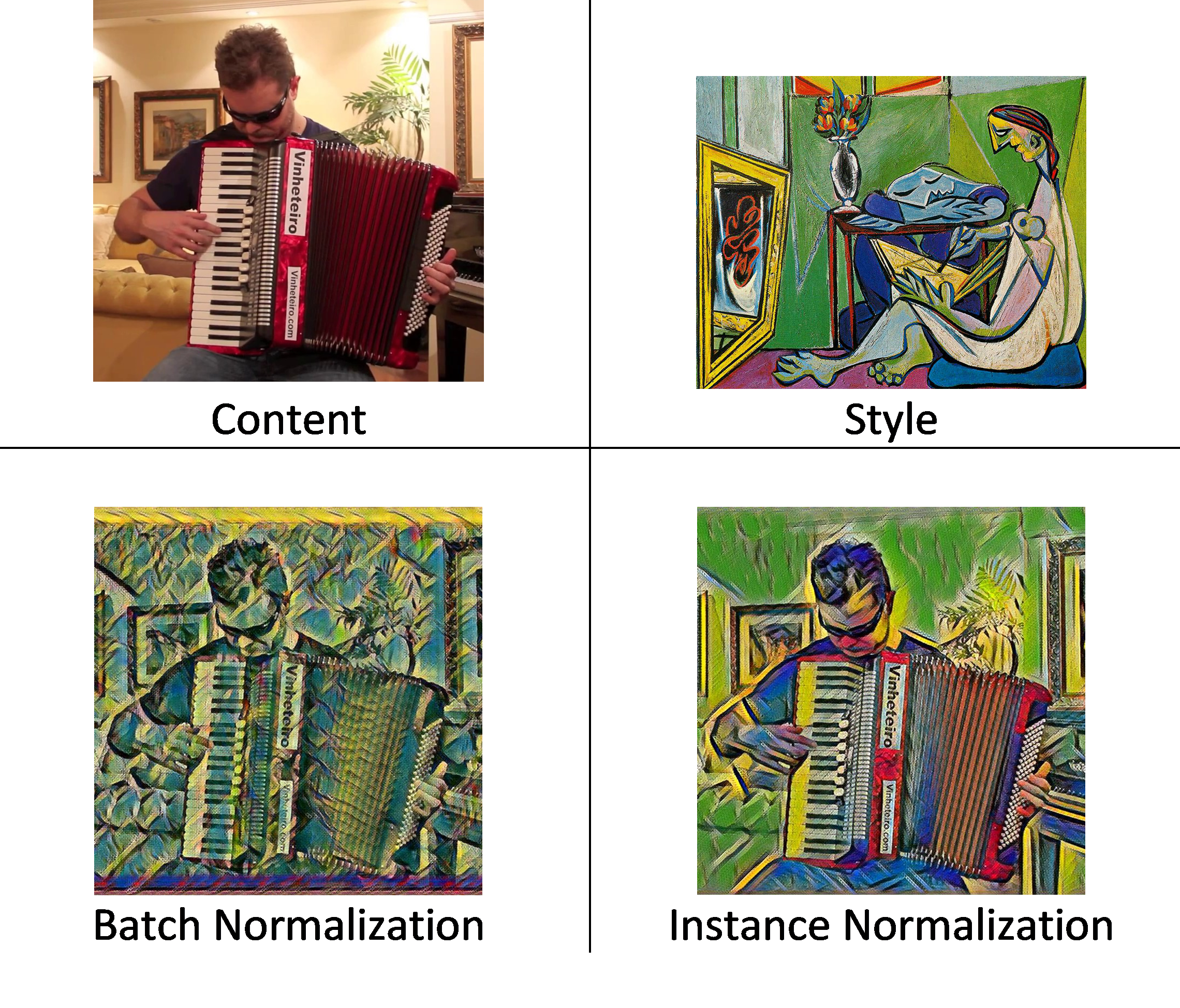
Figure 2: Stylized image using batch and instance normalization. Instance normalization improves the production quality.

4.2 Visualization

Fig.  3 and Fig.  4 demonstrate style transferred images on MPII. More details are in Sec.  4.4.1 and here .

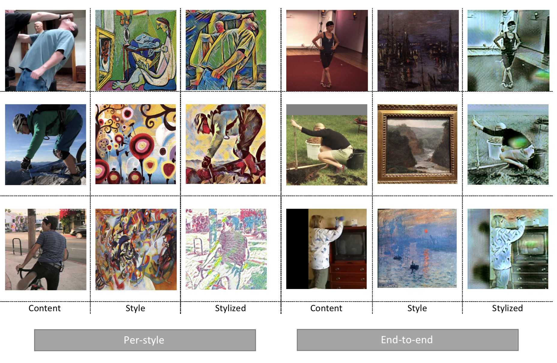
Figure 3: Visualization of style transferred images.

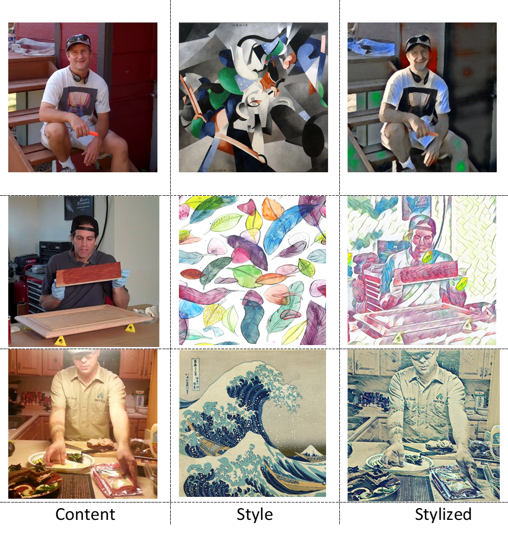
Figure 4: Per-style stylization.

We show 2d keypoints prediction in Fig.  5. We simultaneously present regressed 2d and 3d poses in Fig.  6, where 2d poses are plotted in the small windows. We can see that the 2d and 3d predictions are reasonable.

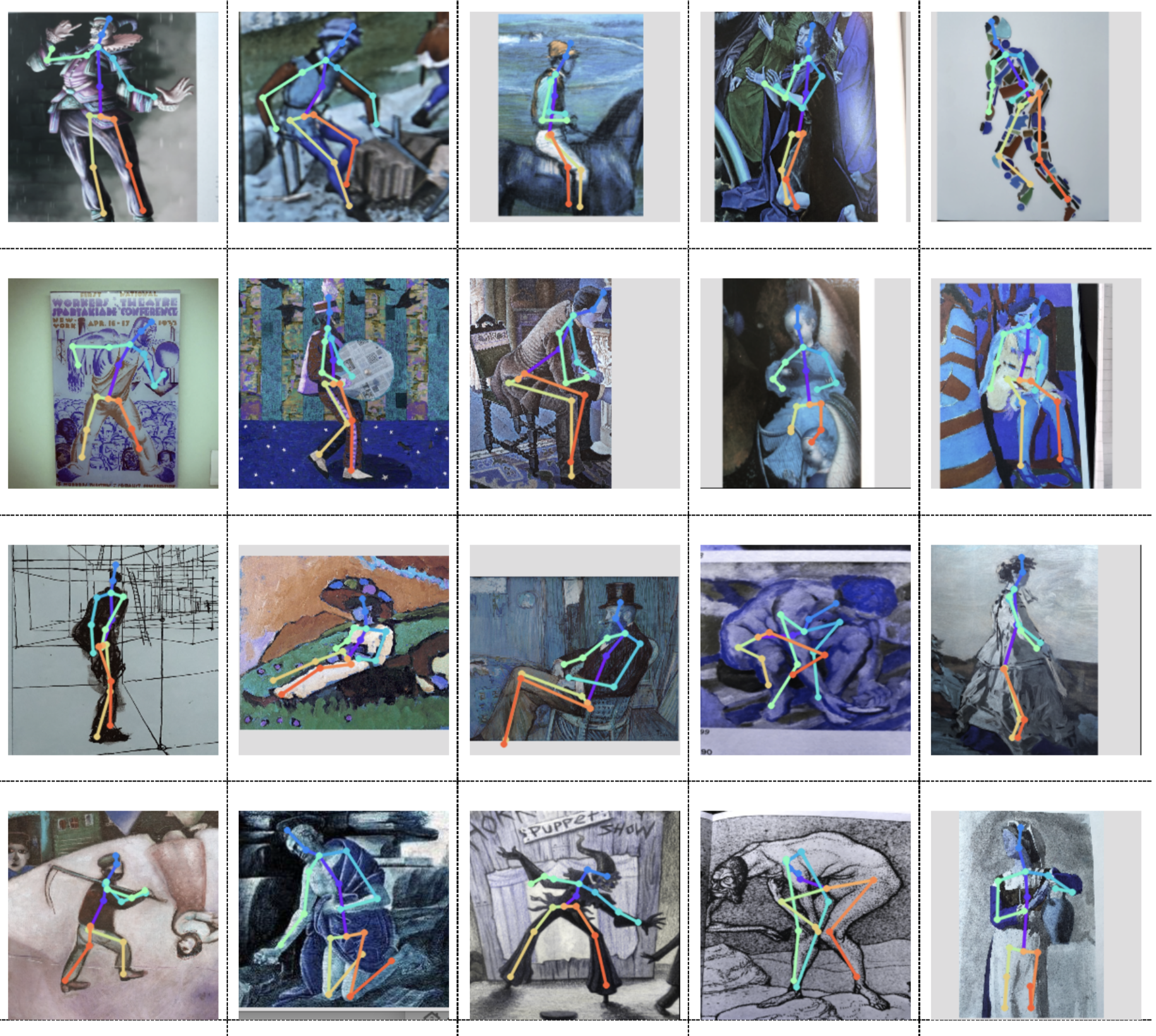
Figure 5: 2d pose predictions on the test set.

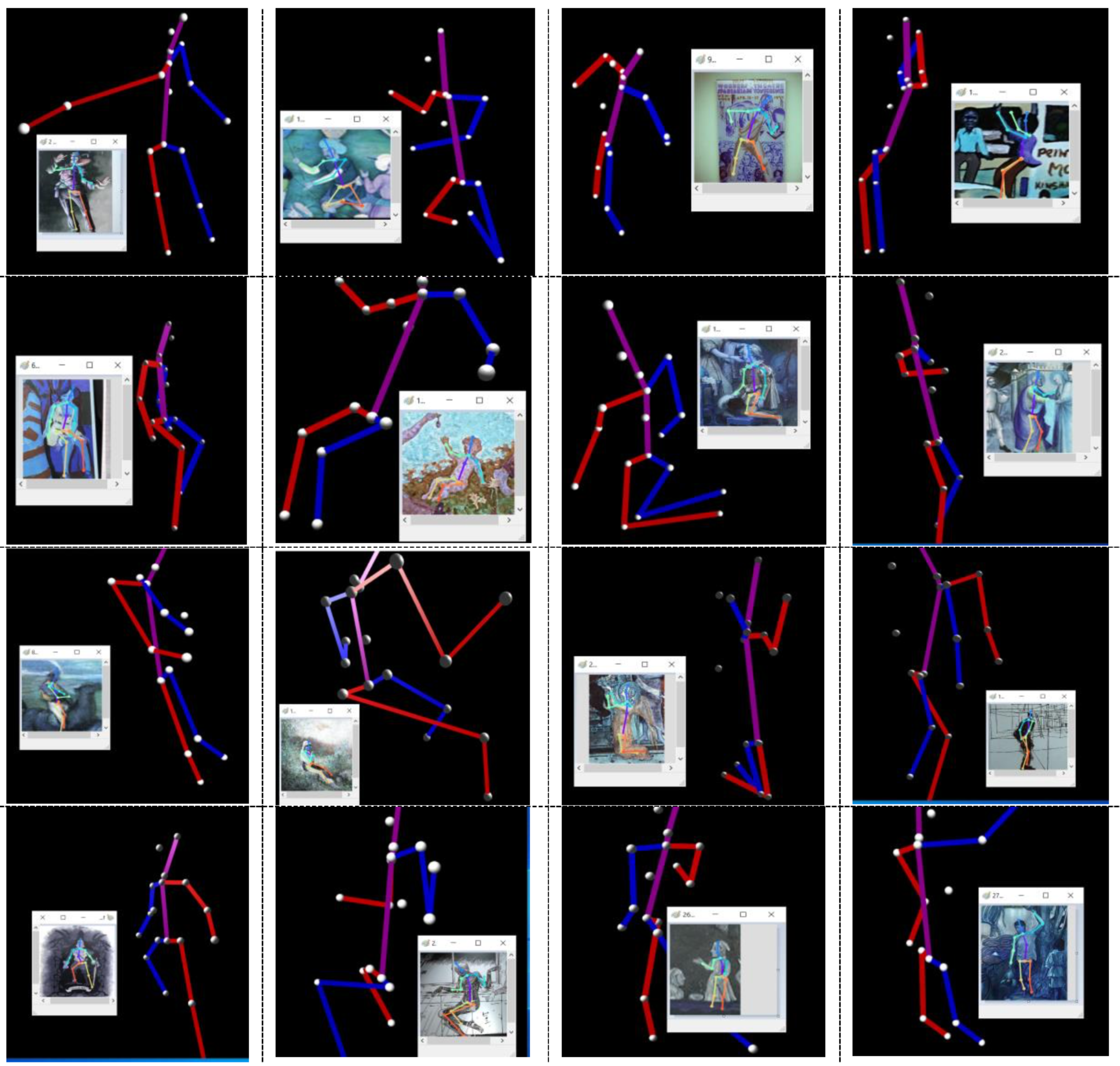
Figure 6: 2d and 3d predictions on the test set.

4.3 State-of-the-art Comparison

There is no existing work tackling estimation of 3d poses in art images that include a human figure. In this part, we apply top-performing methods trained on real-world datasets to our test set. Results are visualized in Fig.  7. One can easily spot misplaced joints of these methods, which may be attributed to different image domains, lack of diverse pose labels (Appendix Sec. E).

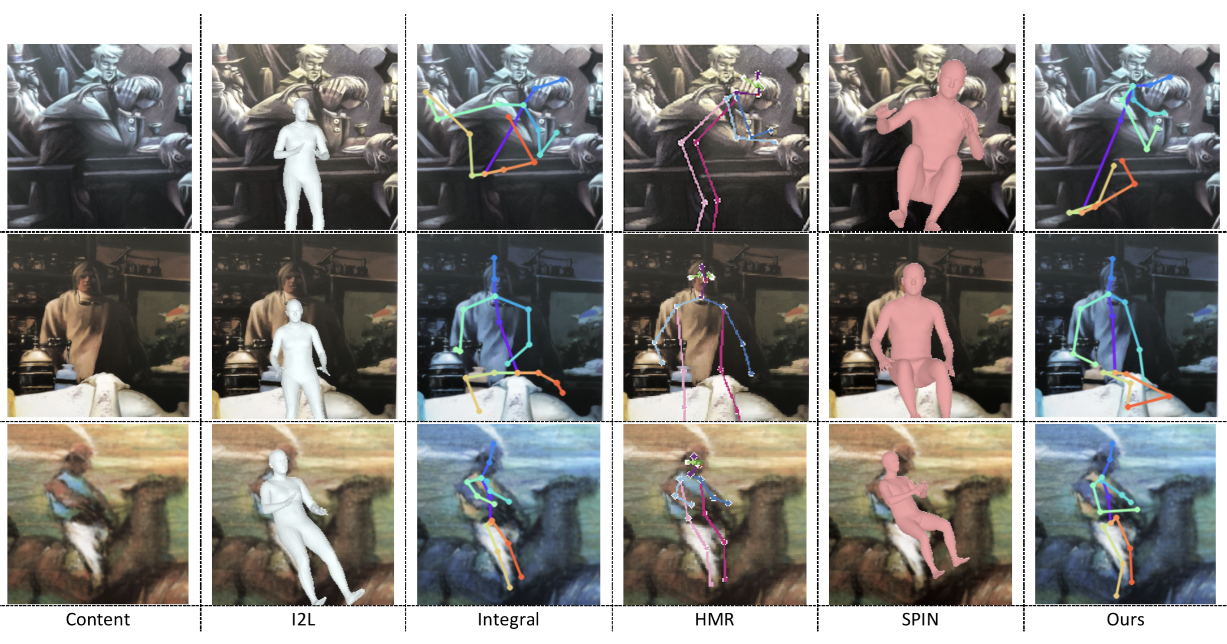
Figure 7: Comparison with state-of-the-art methods. I2L: [21], Integral: [25], HMR: [13], SPIN: [14]. Ours: our full pipeline.

4.4 Ablation

4.4.1 End-to-end Training vs Per-style Training

Per-style training produces more pleasing stylization images than joint-training. In Fig.  3, the left $3$ columns correspond to this style-specific training. However, in terms of pose accuracy, end-to-end performs better. To reflect this, we evaluate PCKh@0.25 and draw Table.  1.

Joint	w/o style	la_muse	3 styles	5 styles	9 styles	12 styles	ours
Ankle	21.4	21.5	24.7	23.8	24.6	26.0	31.0
Knee	23.0	33.5	32.4	31.3	32.0	31.0	25.3
Wrist	30.9	30.1	31.7	32.4	32.4	33.4	37.7
Elbow	33.1	33.7	34.0	35.7	35.2	35.9	44.4
Shoulder	41.0	43.0	43.0	43.7	42.5	41.2	55.8
Head	52.9	51.2	55.1	55.3	55.6	55.6	58.9
Hip	19.4	21.7	21.2	22.1	23.0	23.5	25.8
Total	34.5	35.3	36.9	37.4	37.6	37.9	44.4

Table 1: PCKh@0.25 (%) (the higher, the better) of style-specific training vs arbitrary style joint training. la_muse: test the model trained with only style la_muse. $N$ styles : average the predictions of $N$ style-specific models on the test set. ours: the full end-to-end pipeline.

4.4.2 Style Transfer Losses

Continuing the investigation on style transfer, we now move on to the extra losses introduced. As seen in Fig.  8, adding HSV loss gears the stylized image towards a warm tone, consistent with the style image. The cosine loss encourages the stylized image to be perceptually similar to the style image in high-level layers but does not necessarily require an exact match. Comparing images in another color space sRGB further boosts the stylized image quality.

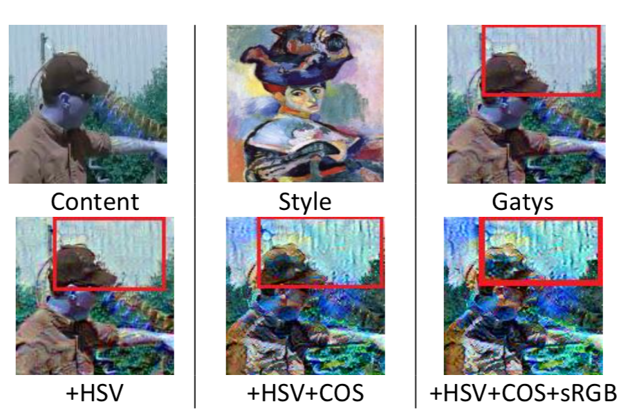
Figure 8: Stylized image using different style losses. Adding more improves the production quality. Gatys: [7].

4.4.3 Pseudo 3d Ground Truth

The pose regression part starts to analyze the pose after the stylization is done. As pointed out, to extend the 3d pose variety (Appendix Sec. E) we manually annotate the pseudo 3d labels of the full MPII. To signify its importance, we compare the predictions trained with and without these labels in Fig.  9. In row 1, the left arm is closer to the camera than the right one, which is correctly captured by the model trained with pseudo 3d labels of MPII. In row 2, the model preserves the lunge pose with the aid of pseudo 3d labels. Further, in row 3 the arm prediction without using pseudo 3d labels is arbitrary, whereas the one with pseudo 3d labels is only incognizant of the forward-leaning left arm.

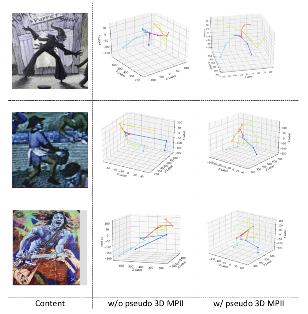
Figure 9: Visualization of 3d pose predictions with and without the pseudo 3d ground truth of MPII.

4.4.4 Bone Map

Extending the discussion on pose regression, here we try to answer how the proposed bone map benefits the depth estimation. Fig.  10 exhibits the pose with and without bone map. It is not hard to observe the mistakes are fixed with the usage of bone map.

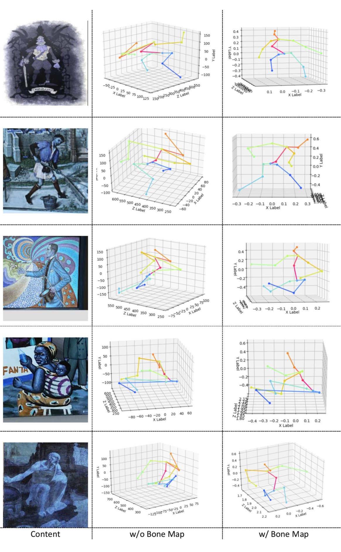
Figure 10: 3d results with and without bone map.

4.4.5 Self Supervision

The self supervision explicitly improves the 2d pose, which we measure by comparing the PCKh@0.25 of the model with and without self supervision. Looking at Table  2, it is most effective for improving upper body joints $i.e.$ elbow, wrist, shoulder and head, which is understandable since upper body joints are generally easier to estimate. Be aware of that PCKh@0.25 is a stricter threshold than the commonly used PCKh@0.5, but the following is true: self supervision leads to non-trivial improvements. Appendix Sec. I.2 reflects the property of the bone map space $\mathcal{P}$ and expresses the bone map from fundamental groups.

Joint	w/o self_sup	w/ self_sup
Ankle	28.9	29.4
Knee	30.7	31.1
Wrist	34.7	38.7
Elbow	41.3	44.4
Shoulder	48.1	49.5
Head	58.3	60.2
Hip	27.0	27.3
Total	41.7	43.0

Table 2: PCKh@0.25 (%) between the model trained with and without self supervision. The higher, the better.

4.5 Cross-dataset Generalization

In this section we will take an excursion into generalizing to another domain: real-world images. The main focus of the project is to evaluate on artistic style human images, yet we would also like to see how it will adapt to real human figures. For this purpose, we apply the model trained exclusively on stylized images to H36M. The MPJPE (w/ Procrustes Alignment) is 82.91 $mm$. It is certainly much worse than state-of-the-art works, but do note that H36M dataset is not used anywhere for this setting. Recall in Sec.  4.3 we apply methods trained on real images to our artistic test set. One interesting question to ask then would be, what would happen if we include both real images and artistic images in training? We adjust the ratio between real and art images in training pose network $\mathcal{G}$, which means a random portion of $\mathbf{O}$ will be replaced with the original RGB $\mathbf{I}$. We load weights of the main system and fine tune from there. (Appendix Sec. H) In Table.  3, we see naturally using more real images leads to better accuracy on H36M. Yet we find the result on our test set is only slightly improved. Since the depth is estimated from the bone map by decoupling, we do not see a significant boost. However, having said that, including images from both real and artistic domain would be conducive if we demand a generic pose model that works on any images containing a human. (See Appendix Sec. G)

Real:stylized ratio	H36M PA MPJPE	PCKh@0.25
10%	91.6	41.8
30%	71.8	44.5
50%	63.5	45.5
70%	67.4	42.7

Table 3: Quantitative effect on H36M and our test set of different real:artistic ratios. PA MPJPE (mm): the lower the better. PCKh@0.25 (%): the higher the better.

5 Conclusion

We present the first method to estimate 3d human poses in artworks. We show considerably well results in varied cases. Key to our approach is the customization of neural style transfer and the exploration of pose regression. We exploit neural style transfer to (a) stylize real images for pose regression (b) self supervise 2d pose predictions. We create a solid baseline using per-style training with instance normalization and exhibit notable stylized image collections. Notice this already gives strong pose results. For further improvement, we build an end-to-end system featuring novel style losses, self supervision, bone map. We infuse the system with a self-collected style set and self-annotated pseudo 3d labels of MPII. We build a test set for evaluation and ablation. Along the way, we elevate the system to a generic pose model with real/art balancing. Theory comes up next.

References

- [1] Ijaz Akhter and Michael J Black. Pose-conditioned joint angle limits for 3d human pose reconstruction. In Proceedings of the IEEE conference on computer vision and pattern recognition, pages 1446–1455, 2015.
- [2] Mykhaylo Andriluka, Leonid Pishchulin, Peter Gehler, and Bernt Schiele. 2d human pose estimation: New benchmark and state of the art analysis. In Proceedings of the IEEE Conference on computer Vision and Pattern Recognition, pages 3686–3693, 2014.
- [3] Christoph Bregler and Jitendra Malik. Tracking people with twists and exponential maps. In Proceedings. 1998 IEEE Computer Society Conference on Computer Vision and Pattern Recognition (Cat. No. 98CB36231), pages 8–15. IEEE, 1998.
- [4] Yucheng Chen, Yingli Tian, and Mingyi He. Monocular human pose estimation: A survey of deep learning-based methods. Computer Vision and Image Understanding, 192:102897, 2020.
- [5] Pedro Felzenszwalb, David McAllester, and Deva Ramanan. A discriminatively trained, multiscale, deformable part model. In 2008 IEEE conference on computer vision and pattern recognition, pages 1–8. IEEE, 2008.
- [6] E.F. Fry. Cubism. World of art. Oxford University Press, 1978.
- [7] Leon A Gatys, Alexander S Ecker, and Matthias Bethge. Image style transfer using convolutional neural networks. In Proceedings of the IEEE conference on computer vision and pattern recognition, pages 2414–2423, 2016.
- [8] Shreyank N. Gowda and Chun Yuan. Colornet: Investigating the importance of color spaces for image classification. CoRR, abs/1902.00267, 2019.
- [9] Ikhsanul Habibie, Weipeng Xu, Dushyant Mehta, Gerard Pons-Moll, and Christian Theobalt. In the wild human pose estimation using explicit 2d features and intermediate 3d representations. In Proceedings of the IEEE Conference on Computer Vision and Pattern Recognition, pages 10905–10914, 2019.
- [10] Catalin Ionescu, Dragos Papava, Vlad Olaru, and Cristian Sminchisescu. Human3.6m: Large scale datasets and predictive methods for 3d human sensing in natural environments. IEEE Transactions on Pattern Analysis and Machine Intelligence, 36(7):1325–1339, jul 2014.
- [11] Tomas Jenicek and Ondřej Chum. Linking art through human poses. In 2019 International Conference on Document Analysis and Recognition (ICDAR), pages 1338–1345. IEEE, 2019.
- [12] Justin Johnson, Alexandre Alahi, and Li Fei-Fei. Perceptual losses for real-time style transfer and super-resolution. In European conference on computer vision, pages 694–711. Springer, 2016.
- [13] Angjoo Kanazawa, Michael J Black, David W Jacobs, and Jitendra Malik. End-to-end recovery of human shape and pose. In Proceedings of the IEEE Conference on Computer Vision and Pattern Recognition, pages 7122–7131, 2018.
- [14] Nikos Kolotouros, Georgios Pavlakos, Michael J Black, and Kostas Daniilidis. Learning to reconstruct 3d human pose and shape via model-fitting in the loop. In Proceedings of the IEEE International Conference on Computer Vision, pages 2252–2261, 2019.
- [15] Jogendra Nath Kundu, Siddharth Seth, Varun Jampani, Mugalodi Rakesh, R Venkatesh Babu, and Anirban Chakraborty. Self-supervised 3d human pose estimation via part guided novel image synthesis. In Proceedings of the IEEE/CVF Conference on Computer Vision and Pattern Recognition, pages 6152–6162, 2020.
- [16] Shichao Li, Lei Ke, Kevin Pratama, Yu-Wing Tai, Chi-Keung Tang, and Kwang-Ting Cheng. Cascaded deep monocular 3d human pose estimation with evolutionary training data. In Proceedings of the IEEE/CVF Conference on Computer Vision and Pattern Recognition, pages 6173–6183, 2020.
- [17] Tsung-Yi Lin, Michael Maire, Serge Belongie, James Hays, Pietro Perona, Deva Ramanan, Piotr Dollár, and C Lawrence Zitnick. Microsoft coco: Common objects in context. In European conference on computer vision, pages 740–755. Springer, 2014.
- [18] Chenxu Luo, Xiao Chu, and Alan Yuille. Orinet: A fully convolutional network for 3d human pose estimation. arXiv preprint arXiv:1811.04989, 2018.
- [19] Prathmesh Madhu, Tilman Marquart, Ronak Kosti, Peter Bell, Andreas Maier, and Vincent Christlein. Understanding compositional structures in art historical images using pose and gaze priors. arXiv preprint arXiv:2009.03807, 2020.
- [20] Prathmesh Madhu, Angel Villar-Corrales, Ronak Kosti, Torsten Bendschus, Corinna Reinhardt, Peter Bell, Andreas Maier, and Vincent Christlein. Enhancing human pose estimation in ancient vase paintings via perceptually-grounded style transfer learning, 2020.
- [21] Gyeongsik Moon and Kyoung Mu Lee. I2l-meshnet: Image-to-lixel prediction network for accurate 3d human pose and mesh estimation from a single rgb image. arXiv preprint arXiv:2008.03713, 2020.
- [22] Greg Mori and Jitendra Malik. Estimating human body configurations using shape context matching. In European conference on computer vision, pages 666–680. Springer, 2002.
- [23] Mohamed Omran, Christoph Lassner, Gerard Pons-Moll, Peter Gehler, and Bernt Schiele. Neural body fitting: Unifying deep learning and model based human pose and shape estimation. In 2018 international conference on 3D vision (3DV), pages 484–494. IEEE, 2018.
- [24] Xiao Sun, Jiaxiang Shang, Shuang Liang, and Yichen Wei. Compositional human pose regression. In Proceedings of the IEEE International Conference on Computer Vision, pages 2602–2611, 2017.
- [25] Xiao Sun, Bin Xiao, Fangyin Wei, Shuang Liang, and Yichen Wei. Integral human pose regression. In Proceedings of the European Conference on Computer Vision (ECCV), pages 529–545, 2018.
- [26] Dmitry Ulyanov, Andrea Vedaldi, and Victor Lempitsky. Instance normalization: The missing ingredient for fast stylization. arXiv preprint arXiv:1607.08022, 2016.
- [27] Qingfu Wan, Weichao Qiu, and Alan L Yuille. Patch-based 3d human pose refinement. In CVPRW, 2019.
- [28] Qingfu Wan, Wei Zhang, and Xiangyang Xue. Deepskeleton: Skeleton map for 3d human pose regression. arXiv preprint arXiv:1711.10796, 2017.
- [29] Christopher Richard Wren, Ali Azarbayejani, Trevor Darrell, and Alex Paul Pentland. Pfinder: Real-time tracking of the human body. IEEE Transactions on pattern analysis and machine intelligence, 19(7):780–785, 1997.
- [30] Xingyi Zhou, Xiao Sun, Wei Zhang, Shuang Liang, and Yichen Wei. Deep kinematic pose regression. In European Conference on Computer Vision, pages 186–201. Springer, 2016.