A scalable control design for grid-forming inverters in microgrids

Abstract

Microgrids are increasingly recognized as a key technology for the integration of distributed energy resources into the power network, allowing local clusters of load and distributed energy resources to operate autonomously. However, microgrid operation brings new challenges, especially in islanded operation as frequency and voltage control are no longer provided by large rotating machines. Instead, the power converters in the microgrid must coordinate to regulate the frequency and voltage and ensure stability. We consider the problem of designing controllers to achieve these objectives. Using passivity theory to derive decentralized stability conditions for the microgrid, we propose a control design method for grid-forming inverters. For the analysis we use higher-order models for the inverters and also advanced dynamic models for the lines with an arbitrarily large number of states. By satisfying the decentralized condition formulated, plug-and-play operation can be achieved with guaranteed stability, and performance can also be improved by incorporating this condition as a constraint in corresponding optimization problems formulated. In addition, our control design can improve the power sharing properties of the microgrid compared to previous non-droop approaches. Finally, realistic simulations confirm that the controller design improves the stability and performance of the power network.

I Introduction

Microgrids are a key technology for the integration of distributed energy resources (DER) into the power network. These distributed energy resources are connected to the network via power converters. The microgrid concept allows local clusters of loads, distributed generation, and energy storage systems to operate together in smaller electrical networks, either in grid-connected mode or autonomously. The potential benefits are considerable, including reduced capital costs, increased efficiency and reliability. However, microgrid operation brings new challenges of its own, since power converters have contrasting dynamical behavior to rotating machines with large inertia [1]. In islanded operation, frequency and voltage control are no longer provided by large rotating machines. Instead, the power converters in the microgrid must regulate the frequency and voltage themselves, while ensuring stability. Furthermore, they must share the power requirement between the converters to avoid exceeding ratings.

Traditionally, droop control has been used for inverters in microgrids, usually in terms of active power-frequency droop and reactive power-voltage droop [2]. These take their inspiration from similar mechanisms built into the governors and exciters of synchronous generators. Droop controllers are practical, simple, and operate entirely on local measurements. However, they suffer from several issues, including frequency and voltage deviations depending on the load and poor transient performance in some situations [3] [4]. Analytical studies also often incorporate additional assumptions, such as simplified inverter models or static/lossless lines, to guarantee stability in a decentralized way in general network topologies. Another possible droop approach for stabilizing inverter-based power systems is angle droop control [5], and the closely related virtual impedance technique [6]. In our previous work [4], these schemes were compared and the difficulty of guaranteeing stability in these schemes via decentralized passivity-based conditions was shown.

Non-droop approaches typically require a Power Measurement System (PMS) which solves an optimal power flow (OPF) problem for the entire microgrid at specified intervals and communicates appropriate setpoints to each inverter. While this requires additional communication between the PMS and each inverter, better transient performance may be achieved along with optimal steady-state power allocations. The accuracy of the load sharing is dependent on how often the optimal power flow is solved [8], and the grid frequency is fixed by internal oscillators which are periodically synchronized. Proposed approaches include $H_{\infty}$ controllers [9], two-degrees-of-freedom control [10], robust servomechanism controllers [11], and LMI-based state feedback [12]. However, some of these approaches require retuning to integrate new devices and many do not take the dynamical nature of the distribution lines into account. In [8] polytopic uncertainty was used to achieve plug-and-play capability without this requirement for retuning; however, an assumption that certain coupling terms between the inverters can be neglected is required, which in practice may not always be satisfied. In [20], a port-Hamiltonian formulation was used to achieve plug-and-play stabilization of the microgrid. One general drawback of many of the non-droop approaches is that during the period between the load change and the new OPF broadcast, proportional power sharing cannot be guaranteed [8], and these schemes are usually unable to successfully operate in the case of communication failure.

In this paper, we aim to combine the advantages of both droop and non-droop approaches by means of a control design which, similarly to the non-droop controllers, is synchronized to the other inverters in the network via a PMS. However, by designing a virtual impedance that exemplifies angle droop-like behavior [6], we also allow the power requirements to be shared in the time between setpoint broadcasts. Compared to previous work [7] using virtual impedance and a PMS, we design novel controllers for which we are able to guarantee stability in a decentralized way. We use passivity theory for this stability guarantee. In order to apply passivity approaches to AC power networks, the choice of an appropriate frame of reference for representing the network dynamics requires consideration. Many approaches for stability analysis have focused on models formulated in a local reference frame. However, for the network to be passive this typically requires the assumption of lossless static lines. An alternative approach is to use the Park and Clarke transformations in a common reference frame [15], since in this frame of reference transmission lines retain their natural passivity properties, without having to resort to a lossless assumption or omit their dynamic behavior. This frame of reference is often used in the literature for grid-connected voltage-source converters (VSCs), e.g. [16], and its significance in inverter-based grids was also pointed out in [4]. In terms of microgrids with grid-forming inverters, the key contribution of [18] showed that the same passivity property leads to network stability. Compared to this and other work in the literature, our virtual impedance approach allows to establish strict passivity while providing power sharing. Furthermore, we exploit the LMI formulation for passivity to formulate optimization problems which can lead to static as well as high-order dynamical controllers that satisfy additional performance criteria.

Paper contributions

This paper considers the problem of control design for grid-forming inverters which guarantees stability and plug-and-play operation via passivity in a common reference frame, while still having appropriate properties that facilitate power-sharing and voltage regulation. The main contributions of this work may be summarized as follows:

1. We propose a control design for grid-forming inverters which ensures plug-and-play capability by satisfying a decentralized passivity criterion. In particular, the proposed controllers provide stability guarantees for the microgrid using a general dynamic model for the lines and a higher-order model for the inverters.

2. The use of passivity as an LMI constraint allows us to formulate optimization problems with various objectives or other constraints to improve performance. This can lead to various controllers that preserve the passivity property, such as a dynamic controller that satisfies mixed $H_{\infty}$/passivity conditions.

3. Our control strategy, via its droop-like behavior, allows contributions from multiple inverters to regulate disturbances even before new setpoints are broadcast.

4. A case study using detailed simulations is used to verify the performance of the proposed controllers, demonstrating the very good performance of an inverter-based microgrid with the proposed controllers.

Paper outline

The paper is organized as follows: in Section II we present preliminaries, introduce the models used, and discuss the passivity condition for the stabilization of the network. In Section III we present our control design. Simulations presented in Section IV show how the dynamic response of the system is improved by our passivity-based design. Finally, Section V summarizes our conclusions.

II Preliminaries and models

II-A Notation and definitions

A power system is comprised of buses (generators, loads, etc.) and lines, which we represent as a graph $(N,E)$ where $N$ is the set of buses $\{1,2,\dots|N|\}$ and $E\subset N\times N$ is the set of edges (lines). A direction is assigned to each edge which can be arbitrarily chosen.

In this paper, we use the well-known Park and Clarke transformations to transform a balanced AC signal $x_{abc}$ into its $DQ$ components in a common reference frame with constant synchronous frequency $\omega_{{\color[rgb]{0,0,0}s}}$. The transformation $T(\omega_{{\color[rgb]{0,0,0}s}}t)$ we adopt is the power invariant form, which aligns the D-axis with the inverter terminal voltage.

$$T(\omega_{{\color[rgb]{0,0,0}s}}t)=\sqrt{\frac{2}{3}}\begin{bmatrix}\cos(\omega_{{\color[rgb]{0,0,0}s}}t)&\cos(\omega_{{\color[rgb]{0,0,0}s}}t-\frac{2\pi}{3})&\cos(\omega_{{\color[rgb]{0,0,0}s}}t+\frac{2\pi}{3})\\ \sin(\omega_{{\color[rgb]{0,0,0}s}}t)&\sin(\omega_{{\color[rgb]{0,0,0}s}}t-\frac{2\pi}{3})&\sin(\omega_{{\color[rgb]{0,0,0}s}}t+\frac{2\pi}{3})\end{bmatrix}$$

$${\color[rgb]{0,0,0}x_{DQ}=T(\omega_{{\color[rgb]{0,0,0}s}}t)x_{abc}}$$

The voltage at a bus $j\in N$ is denoted by $v^{j}_{DQ}$, the summation of the currents flowing out of that bus into one or more edges (i.e. what is often called the “current injection” of that bus to the network) is denoted by $i^{j}_{DQ}$. We will use $V_{DQ}=[v^{j}_{DQ}]_{j\in N}$, $I_{DQ}=[i^{j}_{DQ}]_{j\in N}$ to denote the vectors of all DQ bus voltages and current injections, respectively. $I_{n}$ denotes the $n\times n$ identity matrix, $J$ the matrix $\begin{bmatrix}0&1\\ -1&0\end{bmatrix}$, $\otimes$ denotes the Kronecker product, and $\Re[z]$ denotes the real part of a complex number $z$. Throughout the paper, the equilibrium value of a variable $x$ is denoted by an asterisk superscript $x^{*}$, the eigenvalues of a matrix $A$ are denoted by $\lambda_{i}(A)$ and the maximum singular value by $\bar{\sigma}(A)$. We use $\text{diag}(x)$ to denote the diagonal matrix with the elements of the vector $x$ on the diagonal, and bdiag to denote the analogous operation for block diagonal matrices.

II-B Line dynamics

We model the transmission/distribution lines as RLC components and assume that the network is three-phase balanced in all lines and at all buses. The dynamical equations in the $DQ$ frame are easily derived by applying the Park-Clarke transformation to the fundamental equations of the individual components. We write these equations in a general form, where lines are represented with a distributed parameter model with an arbitrarily large number of states and with the line parameters allowed to vary along the lines, as illustrated in Fig. 1. It should be noted that the simpler lumped model for transmission lines is a special case of this model and it is also known that this tends to the telegrapher equations as the number of elementary sections tends to infinity.

Fig. 1: Transmission line model.

In particular, each line $(i,j)\in E$ has $n$ subsections, where $n$ can be an arbitrarily large number (the stability conditions that will be presented are independent of $n$). Each subsection $k$ has resistance/inductance/conductance/capacitance $R^{ij}_{k},L^{ij}_{k},G^{ij}_{k},C^{ij}_{k}$ respectively, as shown in Fig. 1, and the line equations in DQ coordinates are:

$${\small\begin{matrix}L^{ij}_{1}\dot{I}^{ij}_{DQ,1}&=&-R^{ij}_{1}I^{ij}_{DQ,1}+{\color[rgb]{0,0,0}\omega_{s}}L^{ij}_{1}JI^{ij}_{DQ,1}+V^{i}_{DQ}-V^{ij}_{DQ,1}\\ C^{ij}_{1}\dot{V}^{ij}_{DQ,1}&=&-G^{ij}_{1}V^{ij}_{DQ,1}+\omega_{s}C^{ij}_{1}JV^{ij}_{DQ,1}+I^{ij}_{DQ,1}-{\color[rgb]{0,0,0}I^{ij}_{DQ,2}}\\ &\vdots&\\ L^{ij}_{n}\dot{I}^{ij}_{DQ,n}&=&-R^{ij}_{n}I^{ij}_{DQ,n}+\omega_{s}L^{ij}_{n}JI^{ij}_{DQ,n}+V^{ij}_{DQ,n-1}-V^{j}_{DQ}\\[7.74997pt] \end{matrix}}\\$$ (1)

where the inductor current of the $k$th subsection of the line $(i,j)\in E$ is $I^{ij}_{DQ,k}$, the capacitor voltage of the $k$th capacitor of the same line is $V^{ij}_{DQ,k}$, and the terminal (end-point) voltages are $V^{i}_{DQ}$ and $V^{j}_{DQ}$ where $i$ and $j$ are the buses which are connected by the line $(i,j)$.

By defining various incidence matrices $H,H_{B},H_{C}$ (detailed in Appendix A) composed of zeros and ones to simplify the notation, (1) for all lines $(i,j)\in E$ can be represented in matrix form as follows:

$${\small\begin{matrix}[\mathcal{L}\otimes I_{2}]\dot{I}^{\mathcal{N}}_{dq}&=&-[\mathcal{R}\otimes I_{2}+\omega_{s}\mathcal{L}\otimes J]I^{\mathcal{N}}_{dq}+[H_{C}^{T}\otimes I_{2}]V^{C}_{dq}\\ &&\phantom{hi}+[H_{B}^{T}\otimes I_{2}]V_{dq}\\ [\mathcal{C}\otimes I_{2}]\dot{V}^{C}_{dq}&=&-[\mathcal{G}\otimes I_{2}+\omega_{s}\mathcal{C}\otimes J]V^{C}_{dq}+[H_{C}\otimes I_{2}]I^{\mathcal{N}}_{dq}\\ I_{dq}&=&[H_{B}\otimes I_{2}]I^{\mathcal{N}}_{dq}\end{matrix}}\\$$ (2)

where $\omega_{{\color[rgb]{0,0,0}s}}$ is the constant synchronous frequency, and $\mathcal{R},\mathcal{L},\mathcal{G},\mathcal{C}$ are diagonal matrices of the line resistances, inductances, conductances, and capacitances respectively. As stated in Section II-A, $I_{DQ}$ and $V_{DQ}$ represent the vector of currents drawn from each bus, and the bus voltages respectively.

Note that at each bus $j$, the current injected into the network $i^{j}_{DQ}$ and the bus voltage $v^{j}_{DQ}$ are related by the bus dynamics, which in this study will include the inverter dynamics discussed in Section II-C.

II-C Bus dynamics

We consider now the bus dynamics. As mentioned earlier, there are two types of buses: generation and load. The main focus of this paper is the generation buses where we design controllers to ensure stability together with some performance requirements. We discuss allowable load buses and load dynamics in Section 1, Remark 4. The converter dynamics at generation buses are allowed to be different at each bus $j$, however the bus index $j$ will be omitted for convenience in the presentation.

Assumption 1

We use an averaged inverter model with a stiff DC voltage. We also assume that harmonics can be ignored.

The inverter models in this paper are LC-filtered. We use $v_{iDQ}$ to refer to the inverter voltage which is the control input to the inductive filter, and $v_{DQ}$ is the capacitor voltage. Similarly, the current entering the LC filter from the DC-side is $i_{iDQ}$ and the current leaving the filter (injected into the network) is $i_{DQ}$. Fig. 2 illustrates the voltages and currents used in the model.

Fig. 2: Inverter filter circuit diagram, showing the notation and current direction convention used in this paper. The inverter itself is connected on the left, with $v_{iDQ}$ representing the inverter voltage behind the filter.

Using Assumption 1, the converter dynamics may be represented as a linear system of the form:

$$\begin{matrix}\dot{x}&=\mathcal{A}x+\mathcal{B}_{u}u+\mathcal{B}_{w}w\\ z&={\color[rgb]{0,0,0}\mathcal{C}_{z}}x+\mathcal{D}_{u}u+\mathcal{D}_{w}w\end{matrix}$$ (3)

where the states are $x=[i_{iDQ}^{T}\phantom{i}v_{DQ}^{T}]^{T}$, $u=v_{iDQ}$ is the controlled PWM voltage, and the input current from the network lines is the current $w=-i_{DQ}$ and the output is the voltage vector $z=v_{DQ}$. The system matrices are given by:

$$\mathcal{A} =\begin{bmatrix}-\dfrac{R}{L}&\omega_{{\color[rgb]{0,0,0}s}}&-\dfrac{1}{L}&0\\ -\omega_{{\color[rgb]{0,0,0}s}}&-\dfrac{R}{L}&0&-\dfrac{1}{L}\\ 1/C&0&-\dfrac{G}{C}&\omega_{{\color[rgb]{0,0,0}s}}\\ 0&\dfrac{1}{C}&-\omega_{{\color[rgb]{0,0,0}s}}&-\dfrac{G}{C}\end{bmatrix},\mathcal{B}_{u}=\begin{bmatrix}\dfrac{1}{L}&0\\ 0&\dfrac{1}{L}\\ 0&0\\ 0&0\end{bmatrix}$$ (4)

$$\mathcal{B}_{w} =\begin{bmatrix}0&0\\ 0&0\\ \dfrac{1}{C}&0\\ 0&\dfrac{1}{C}\end{bmatrix},{\color[rgb]{0,0,0}\mathcal{C}_{z}}=\begin{bmatrix}0&0&1&0\\ 0&0&0&1\end{bmatrix},\mathcal{D}_{u}=\mathcal{D}_{w}=\begin{bmatrix}0&0\\ 0&0\end{bmatrix}$$

In order for each inverter to respond to broadcast signals from a PMS, the dynamics may be augmented with an integrator of the form:

$$\dot{\zeta}_{DQ}=v_{DQ}-v_{DQ}^{set}+Zi_{DQ}$$ (5)

where $v_{DQ}^{set}$ is the voltage setpoint from the PMS and $Z$ is a $2\times 2$ matrix of coefficients which determine the terminal voltage as a function of the input current. Previous work, e.g. [8], used pure integral action (i.e $Z=0_{2\times 2}$) to achieve this voltage regulation. In our full-state feedback design we treat $Z$ as a virtual impedance with $Z=R_{V}I_{2}-X_{V}J$, where $R_{V}>0$ and $X_{V}>0$ are the virtual resistance and reactance, respectively. We denote the augmented dynamics as:

$$\begin{matrix}\dot{\tilde{x}}&=\tilde{A}\tilde{x}+\tilde{B}_{u}u+\tilde{B}_{w}w\\ z&=\tilde{C}\tilde{x}+\tilde{D}_{u}u+\tilde{D}_{w}w\end{matrix}$$ (6)

where $\tilde{x}=[i_{iDQ}^{T}\phantom{i}v_{DQ}^{T}\phantom{i}\zeta_{DQ}^{T}]^{T}$ and the system matrices follow from (4)-(5). Our approach using (5) has several advantages over previous approaches. Firstly, power sharing is achieved during unscheduled load changes. The terms in $Z$ are a virtual impedance that allows the power requirement of load changes to be shared among the converters. The power sharing depends on the equivalent impedance at each converter [6]. Supposing the line impedances to be comparatively small, the power allocation will depend mainly on the virtual impedances. Since these can be chosen by design, an appropriate allocation can thus be achieved. In the case that the line impedances are significant, the equivalent impedance at each inverter determines its contribution and a slight inaccuracy will occur, as was analyzed in [7] for example. This can be adjusted to reach an acceptable compromise between power sharing and voltage fluctuations [7]. Secondly, our approach also allows the design of a controller such that a local strict passivity condition is satisfied without excessively high control gains. With a pure integrator, it is actually impossible to achieve strict passivity [18].

Note that any power sharing inaccuracy is temporary as no inaccuracy is introduced into the OPF by our proposed approach as long as the virtual impedance $Z$ at each inverter is known to the PMS. The voltage setpoints $v_{DQ}^{set}$ broadcast to each inverter can simply be adjusted to take into account the effect of $Z$.

II-D Closed-loop representation of the overall system

In this section we discuss how the power system can be viewed as the closed-loop interconnection of dynamical systems representing the bus dynamics and the line dynamics respectively. The bus dynamics are the dynamics at each bus $j\in N$ which relate the aggregate injected current $i^{j}_{DQ}$ to the bus voltage $v^{j}_{DQ}$. If an appropriate inverter is present, these dynamics will include the inverter dynamics given in Section II-C.

More precisely, the line dynamical system has input $V_{DQ}$ and output $I_{DQ}$ and dynamics given by (2). Note (as stated in Section II-B) that $I_{DQ}$ is a vector of the total $DQ$ currents flowing into the network from each bus and $V_{DQ}$ is a similarly ordered vector of the $DQ$ bus voltages. We close the loop by considering bus dynamics with input $-I_{DQ}$ (the negative sign comes from the fact that this is current leaving the network and flowing into the bus) and output $V_{DQ}$. Fig. 3 shows the representation of the power system as a negative feedback interconnection of the bus and line dynamics [15].

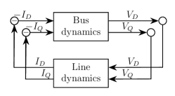
Fig. 3: The power system as an interconnection of bus and line dynamics.

For a bus $j\in N$ at which an inverter is present, Fig. 3 and Fig. 2 are directly related as follows. The input $-i^{j}_{DQ}$ (which is a component of the vector $-I_{DQ}$ as in Fig. 3) is the current $-i_{DQ}$ in Fig. 2. Similarly, the voltage $v^{j}_{DQ}$ (also a component of $V_{DQ}$ in Fig. 3) is the inverter capacitor voltage $v_{DQ}$ in Fig. 2. Therefore every bus has a two-input two-output system associated with it and the direct sum of these systems is denoted as bus dynamics in Fig. 3, i.e. it relates $V_{DQ}$ with $I_{DQ}$ and has a corresponding block diagonal structure.

II-E Passivity

Passivity approaches have been widely used in the literature to achieve network stability in a decentralized and scalable way. Since the negative feedback interconnection of two passive systems is stable and passive [19], by representing the system dynamics as an interconnection of two subsystems and ensuring that both are passive with respect to their inputs and outputs, we can guarantee stability. We consider for each bus $j\in N$ a dynamical system of the form:

$$\begin{matrix}\dot{x_{j}}=f_{j}(x_{j},w_{j})\\ z_{j}=g_{j}(x_{j},w_{j})\end{matrix}$$ (7)

where $f_{j}$ is locally Lipschitz and $g_{j}$ is continuous. The inverter model and line model in this paper are linear, however bus dynamics of some loads or various inverter controllers may be nonlinear and hence we present the bus dynamics in the general form of (7).

Definition 1 (Passivity, [19, Def 6.3]. )

A system as in (7) is said to be locally passive about some equilibrium point $(w_{j}^{*},x_{j}^{*})$ if there exist open neighbourhoods $W_{j}$ of $w_{j}^{*}$ and $X_{j}$ of $x_{j}^{*}$ and a continuously differentiable, positive semi-definite function ${\color[rgb]{0,0,0}\mathcal{V}}_{j}(x_{j})$ such that, for all $w_{j}\in W_{j}$ and all $x_{j}\in X_{j}$:

$$\dot{\mathcal{V}}_{j}\leq(w_{j}-w_{j}^{*})^{T}(z_{j}-z_{j}^{*})$$ (8)

If the property holds with the right hand side of (8) replaced by $(w_{j}-w_{j}^{*})^{T}(z_{j}-z_{j}^{*})-(x_{j}-x_{j}^{*})^{T}\phi_{j}(x_{j}-x_{j}^{*})$, where $\phi_{j}$ is a positive definite function, then the system is said to be locally strictly passive about $(w_{j}^{*},x_{j}^{*})$. If instead the right hand side of (8) is replaced by $(w_{j}-w_{j}^{*})^{T}(z_{j}-z_{j}^{*})-(z_{j}-z_{j}^{*})^{T}\phi_{j}(z_{j}-z_{j}^{*})$, then the system is said to be locally output-strictly passive about $(w_{j}^{*},x_{j}^{*})$. We say that an output-strictly passive system has output-strict passivity index $\rho_{j}>0$ if condition (8) is replaced by:

$${\color[rgb]{0,0,0}\dot{\mathcal{V}}_{j}\leq(w_{j}-w_{j}^{*})^{T}(z_{j}-z_{j}^{*})-(z_{j}-z_{j}^{*})^{T}\rho_{j}(z_{j}-z_{j}^{*})}$$ (9)

Remark 1

It should be noted that if the system (7) is linear then if the passivity property holds locally about an equilibrium point, it also holds globally, i.e., for any other equilibrium point and for any deviation from an equilibrium point. Therefore for linear systems which satisfy Definition 1, we will refer to them as being “passive” (or “strictly passive”) without making reference to a particular equilibrium point.

We start by showing in Proposition 1 that the line dynamical model is passive in a common reference frame, irrespective of its complexity, i.e. for an arbitrarily large number of elementary components used to represent the line dynamics and despite the parameter variation along the lines. This follows from the fact that the lines are composed of passive RLC components and the DQ transform on a common reference frame is an orthogonal transform and thus preserves passivity. The associated proof may be found in Appendix B.

Proposition 1 (Passivity of line dynamical model)

The model of the network lines (2) with input $V_{DQ}-V^{*}_{DQ}$ and output $I_{DQ}-I^{*}_{DQ}$ is strictly passive.

Remark 2

Since the line dynamics are linear, the passivity property holds for any equilibrium point $(V^{*}_{DQ},I^{N\ast}_{DQ})$. However, Proposition 1 does not generally hold when using local $dq$ coordinates due to the different frequencies and angles at various buses. This is a key reason for using a common reference frame for control of every inverter in the network.

Given the result in Proposition 1, passivity allows us to guarantee the stability of the general power network if all the bus dynamics are passive in the common reference frame. We state this result formally in Theorem 1 and the proof is provided in Appendix C.

Assumption 2

We assume that the bus dynamical systems satisfy an output-strict passivity property of Definition 1 about an equilibrium $(w_{j}^{*},x_{j}^{*})$ for each bus $j\in N$. The storage function $\mathcal{V}_{j}(x_{j})$ is continuous and has a strict local minimum at $x_{j}^{\ast}$. We further assume that for a constant input $w_{j}^{*}$, the equilibrium $x^{*}_{j}$ is locally asymptotically stable.

Assumption 2 presents a passivity condition that must be satisfied at all buses, including both inverter buses and load buses. The following remarks discuss the significance of Assumption 2 for both generation (inverter) and load buses.

Remark 3

The passivity condition in Assumption 2 must be satisfied at all buses, and our focus is on the generation / inverter buses. We therefore aim to design grid-forming inverter control schemes which satisfy this Assumption, leading to the stability result we will shortly present. In addition, we will discuss how an appropriate control policy can additionally satisfy other conditions for power sharing or performance.

Remark 4

Assumption 2 also has implications for the incorporation of loads in our framework. If the load dynamics satisfy this Assumption, i.e. they are passive about the equilibrium point, they can be incorporated in our analysis. As it is well known, this property is satisfied by a range of loads including constant impedance loads (Z) and some non-linear loads under appropriate conditions [21]. Individual non-passive loads may also be passivated via strictly passive load at the same bus such that the aggregate dynamics are passive. A further possibility is to incorporate the load dynamics with the inverter dynamics at the bus (if such an inverter is present), with the objective of passivating the aggregate bus dynamics by an appropriate inverter control design. The strictness of the passivity property achieved using the control schemes in this paper makes this possible.

Theorem 1 (Stability)

Suppose there exists an equilibrium ${\color[rgb]{0,0,0}q^{\ast}}=(I^{N*}_{DQ},x_{1}^{*},...,x_{|N|}^{*})$ of the interconnected bus dynamics and line dynamics (2), for which the bus dynamics satisfy Assumption 2 for all buses $j\in N$. Then such an equilibrium is asymptotically stable.

Remark 5

The advantage of the stability criterion in Assumption 2 is the fact that it is a fully decentralized condition which allows a wide range of heterogeneous dynamics at each bus, so long as the aggregate dynamics satisfy the passivity condition. Instead of requiring the detailed modeling of the entire system, each bus may have different dynamics which individually satisfy the passivity condition. This is therefore a decentralized and scalable approach.

III Controller design

Even though a passivity condition in a common reference frame is a sufficient decentralized condition for stability, satisfying this property can in general be a non-trivial problem when higher-order bus dynamics are present. This is, for example, reflected in the fact that no simpler droop control scheme for grid-forming inverters in the literature satisfies a decentralized stability condition that leads to a plug and play capability without requiring simplifications in the inverter or line dynamics. In this section we present our proposed control design such that the passivity condition is satisfied along with various other objectives. We first explain the broader framework of the microgrid operation, list our control objectives, and then present the control design.

III-A Microgrid operation and control objectives

A centralized PMS is used to coordinate the inverters, as in other non-droop approaches [8]. The PMS solves the optimal power flow to calculate the appropriate setpoints, which are broadcast to each inverter in the microgrid. Frequency control is open loop and is achieved by means of internal oscillators at the nominal frequency. Since small errors in frequency cause slow drifts and eventual loss of synchronism, in practice an appropriate communication protocol (e.g. using GPS) is used to synchronize these frequencies at a slower timescale. Each inverter therefore operates at the same frequency and is controlled in the same synchronous $DQ$ frame of reference. If no new setpoint is sent to the inverter (e.g. due to communication failure), it will operate autonomously using the embedded virtual impedance approach. This allows our proposed approach to be reliable and flexible.

Given this microgrid context, our control objectives are as follows.

• Ensure some performance requirements. These specifications typically include: voltage reference tracking, restricted control inputs and limited coupling between buses.

• Allow power requirements of unexpected load changes to be shared between multiple inverters.

• Ensure stability for a general network with plug-and-play functionality. This can be guaranteed via Theorem 1 by ensuring the passivity of the bus dynamics.

Remark 6

The significance of the passivity constraint is that adding this to optimization problems associated with control design leads to control policies which provide stability guarantees for the network.

Remark 7

Output-strict passivity is a way to have performance guarantees in the presence of disturbances (e.g. load fluctuations) by means of a restricted $L_{2}$-gain for each bus, e.g. [23, Theorem 2.2.15]. This is a property that can be ensured with output-strict passivity, and is hence one of the reasons for maximizing output-strictness (parameter $\rho$) in the inverter control design is a reasonable performance criterion. Additional performance criteria will be discussed in Sections III-C, IV and validated with simulations.

III-B Full-state feedback design

The full-state feedback for the inverter model (6) is of the form $u=-K\tilde{x}-Mw$ where $K\in\mathbf{R}^{2\times 6}$ and $M\in\mathbf{R}^{2\times 2}$ are gain matrices: two $dq$ control inputs each being a function of the four states of the physical system, two states corresponding to the voltage integrators, and two input feedback terms. This state feedback requires sixteen control gains to be chosen.

Given the passivity property (9), Theorem 2 states a matrix inequality through which this property can be satisfied (e.g. [22]), and the proof is given in Appendix D. As we will show, these inequalities can be added as a constraint to the optimization problems associated with control design to ensure the passivity property (Assumption 2).

Theorem 2

Consider the state feedback controller $u=-K\tilde{x}-Mw$ in conjunction with the dynamics (6). The system with input $w$ and output $z$ satisfies the passivity condition in Assumption 2 and is output-strictly passive with strictness index $\rho$ if there exists a symmetric matrix $P=P^{T}>0$ that satisfies:

$$\begin{bmatrix}A_{c}^{T}P+PA_{c}{\color[rgb]{0,0,0}+}2\rho C_{c}^{T}C_{c}&PB_{c}-C_{c}^{T}{\color[rgb]{0,0,0}+}2\rho C_{c}^{T}D_{c}\\ B_{c}^{T}P-C_{c}{\color[rgb]{0,0,0}+}2\rho D_{c}^{T}C_{c}&2\rho D_{c}^{T}D_{c}-D_{c}^{T}-D_{c}\end{bmatrix}\leq 0\\$$ (10)

where $A_{c}=\tilde{A}-\tilde{B}_{u}K$, $B_{c}=\tilde{B}_{w}-\tilde{B}_{u}M$, $C_{c}=\tilde{C}-\tilde{D}_{u}K$, and $D_{c}=\tilde{D}_{w}-\tilde{D}_{u}M$. Note that in this case $\tilde{D}_{u}$ and $\tilde{D}_{w}$ are zero matrices.

Remark 8

As stated, (10) is a bilinear matrix inequality. However, using the change of variables $Q=P^{-1},Y=KP^{-1}$ and the Schur complement, it can be rearranged as an LMI. We leave this in the BMI form as it allows us to directly place bound on the control gains in $K$ and $M$, which is not straightforward if such a change of variables is applied. We will also discuss convex problems for controller synthesis in the next section.

III-C Mixed $H_{\infty}$/passivity controller design

In order to achieve complex closed-loop specifications for each inverter, we focus on the design of a dynamical controller $\mathcal{K}$

$$\mathcal{K}:\leavevmode\nobreak\ \leavevmode\nobreak\ \leavevmode\nobreak\ \begin{bmatrix}\dot{x}_{K}\\ u\end{bmatrix}=\begin{bmatrix}A_{K}&B_{K}\\ C_{K}&D_{K}\end{bmatrix}\begin{bmatrix}x_{K}\\ y_{\text{control}}\end{bmatrix}$$ (11)

where $x_{K}$ is the controller state vector, $A_{K}$, $B_{K}$, $C_{K}$ and $D_{K}$ are the controller matrices in its state space representation, $u$ is the control input as in (6), and $y_{\text{control}}=[(v^{ref}_{{DQ}})^{T}\leavevmode\nobreak\ -{i}_{DQ}^{T}\leavevmode\nobreak\ i_{iDQ}^{T}\leavevmode\nobreak\ v_{DQ}^{T}]^{T}$ represent the vector of measured signals serving as inputs for the controller $\mathcal{K}$. The virtual impedance is implemented via the reference $v^{ref}_{{DQ}}=v^{set}_{{DQ}}-Zi_{DQ}$. This controller will be designed to ensure the passivity from $-i_{DQ}$ to output $v_{DQ}$ and also other performance requirements expressed as $H_{\infty}$ constraints to shape the frequency responses of appropriate closed-loop transfer functions:

• $T_{v^{ref}_{DQ}\rightarrow e_{DQ}}$ to obtain the desired voltage reference tracking requirements;

• $T_{v^{ref}_{DQ}\rightarrow u}$ to limit the control input magnitudes;

• $T_{-i_{DQ}\rightarrow v_{DQ}}$ and $T_{-i_{DQ}\rightarrow u}$ to ensure restricted coupling between buses.

These control specifications are taken into account using an appropriate choice of weighting filters $W_{e}$, $W_{u}$ and $W_{d}$ (will be discussed more extensively in Section IV-C) such that

$${\small\begin{matrix}&\left\|W_{e}T_{v^{ref}_{DQ}\rightarrow e_{DQ}}\right\|_{\infty}\leq 1&\left\|W_{e}T_{-{i}_{DQ}\rightarrow v_{DQ}}W_{d}\right\|_{\infty}\leq 1\\[3.87498pt] &\left\|W_{u}T_{v^{ref}_{DQ}\rightarrow u}\right\|_{\infty}\leq 1\leavevmode\nobreak\ \leavevmode\nobreak\ \leavevmode\nobreak\ \leavevmode\nobreak\ &\left\|W_{u}T_{-{i}_{DQ}\rightarrow u}W_{d}\right\|_{\infty}\leq 1\leavevmode\nobreak\ \leavevmode\nobreak\ \leavevmode\nobreak\ \end{matrix}}$$

with $\left\|T\right\|_{\infty}$ being the $H_{\infty}$ norm of the linear system $T$ and is defined as

$${\small\left\|T\right\|_{\infty}=\sup_{{\color[rgb]{0,0,0}\omega\geq 0}}\leavevmode\nobreak\ \leavevmode\nobreak\ \overline{\sigma}\left(T(j\omega)\right)}.$$

Therefore, we are interested in designing a controller $\mathcal{K}$ ensuring the output-strict passivity condition from $-{i}_{DQ}$ to $v_{DQ}$ together with the $H_{\infty}$ conditions. These advanced specifications can be formulated as a convex optimization problem with LMI constraints which can be solved efficiently using standard solvers [27]. This LMI formulation is stated in Appendix E (Theorem 3), and discussed further in Section IV-C.

III-D Controller implementation

We illustrate the full-state feedback control design and the mixed $H_{\infty}$/passivity control design in Fig. 4 and Fig. 5. The full-state feedback design is effectively a single-loop design, in contrast to traditional double (inner current / outer voltage) loop design [2]. Single loop controllers are a promising alternative [24] which have been successfully demonstrated, e.g. [25]. The advantages of the single loop are simpler control design and better stability properties [24] which, in our case, can be exploited to guarantee stable plug-and-play operation. Furthermore, although full-state feedback designs are sometimes impractical due to the requirement to obtain full state information, in this case the only measurements required are the filter voltage and currents, which are also necessary for a traditional double PI loop controller.

Fig. 4: Block diagram of the state feedback controller implementation and system.

Fig. 5: Block diagram of the $H_{\infty}$/passivity controller implementation and system. It should be noted that this is a dynamic controller.

The major differences between the controllers in Figs. 4 and 5 are as follows. The state feedback controller is simple and this allows numerically to consider in control synthesis also certain practical constraints which are non-convex. By contrast, the mixed $H_{\infty}$/passivity controller is dynamic and of high order. A main feature of this controller is that it allows $H_{\infty}$ criteria to be satisfied by formulating a convex LMI problem. As always, there are underlying trade-offs: between the simplicity of a static state feedback controller and the flexibility of a high-order dynamic controller; and also between convexity of the optimization problem and the incorporation of certain non-convex constraints which may be useful in practice.

Remark 9

An issue when eschewing classical cascaded PI loops is current limitation for protection, since in most practical designs the current is limited via saturation of the current reference. Virtual impedance is a proven alternative [14] to limit the current and this can be achieved with our design.

Remark 10

Angle droop and virtual impedance are closely related [6]. Compared to angle droop, our approach and control architecture offers several advantages. Firstly, passivity (and thus plug-and-play operation) is guaranteed, whereas angle droop schemes are only passive for small droop gains [4]. Secondly, droop approaches limit the achievable performance due to the presence of only a few tunable parameters.

IV Case studies

IV-A Control specifications

Although stability is guaranteed via the passivity condition, (likewise $L_{2}$ performance by the output-strictness), in practice further specifications are required to achieve good performance. A sensible approach, and the one we adopt, is to ensure good performance in the case of one inverter with a load, and then add constraints to limit output voltage deviations which also has the effect to reduce the coupling between inverters. Although this method does not give general performance guarantees for any network, our investigations indicate that in practice appropriate network-wide transient performance is achieved.

In addition to the passivity constraint, the different performance specifications considered in this paper are as follows.

• Fast convergence of the voltage tracking error.

• Small control input magnitudes.

• Limited coupling between inverters (in the form of loop shaping design in the frequency domain).

These control specifications will be incorporated as constraints in the optimization problem formulation to obtain the desired controllers.

IV-B State feedback controller synthesis

We start with the static state and input feedback controller $u=-K\tilde{x}-Mw$ and look to design appropriate $K$ and $M$. The states of the plant $\tilde{x}$ include four states associated with the inverter filter and two states associated with the integrator. The previous control specifications can be expressed as follows.

• Maximum controller gains: Note that in general some limit of this sort is necessary to prevent a solution with impractically large gains.

• Maximum real part of eigenvalues of $A_{c}$: This determines the speed of the response for each inverter. The speed of the response is chosen to be sufficiently fast, but must be limited to avoid a controller that saturates the inverter’s PWM operation.

• Bound on the frequency response of the bus dynamics with input $-i_{DQ}$ and output $v_{DQ}$: This reduces the coupling between inverters.

It should also be noted that the virtual impedance is also a parameter which can be chosen (discussed previously) and provides a trade-off between voltage regulation and power sharing. The optimization problem may be stated as follows, where $\tilde{n}$ is the number of states

$$\begin{array}[]{c}{\color[rgb]{0,0,0}\underset{K,M,P}{\max}}\phantom{l}\rho,\text{ such that}\\ {\color[rgb]{0,0,0}\eqref{lmi}\text{{\color[rgb]{0,0,0}\mbox{ }holds}}}\\ {\color[rgb]{0,0,0}|K_{ik}|}\leq p_{max}\\ {\color[rgb]{0,0,0}|M_{ik}|}\leq p_{max}\\ \Re[\lambda_{i}(A_{c})]\leq\lambda_{max}\\ \bar{\sigma}(\tilde{C}(j\omega I-A_{C})^{-1}B_{c}+\tilde{D}_{w})\leq|\gamma\frac{\omega_{c}}{j\omega+\omega_{c}}|\text{ for all }\omega\end{array}$$ (12)

Table I: Tuning specifications for the state feedback controller.

Parameter	Value
Maximum controller gains	$p_{max}=125$
Maximum real part of eigenvalue	$\lambda_{max}=-5$
Frequency response (max gain, bandwidth)	$\gamma=1.5$, $\omega_{c}=10^{5}$ rad/s
Virtual impedance	$R_{V}$ = 0.5, $X_{V}$ = 1

We solve the optimization problem numerically, using MATLAB’s $systune$ [26]. This is a non-convex problem, nonetheless the controller obtained satisfies the passivity condition as well as the design specifications discussed before, resulting in a good design.

Using the inverter filter parameters as in Table IV and specifications as in Table I results in a maximized value of $\rho=0.4000$, and the following controller is obtained:

$$\begin{matrix}K=\begin{bmatrix}117.3&1.1&6.3&0.4&40.0&-7.3\\ -2.6&117.2&-2.1&12.9&2.1&72.5\end{bmatrix},\\ {\color[rgb]{0,0,0}M=}\begin{bmatrix}107.8&3.3\\ -1.2&104.7\end{bmatrix}\end{matrix}$$ (13)

In our experience, the problem is generally feasible for reasonable parameter choices. However, there are obvious cases where the problem may not be feasible; for example, specifying a very fast response while bounding the controller gains $p_{max}$ to a low number; or bounding the maximum gain of the frequency response too low. It is also not a feasible problem to have a negative virtual resistance as well as passivity since such constraints are not compatible. Should the problem be infeasible, it is recommended to adjust the parameters (e.g. higher $p_{max}$) or set less ambitious specifications.

Remark 11

The state feedback problem of (12) is non-convex as it involves a BMI and non-convex constraints. Nevertheless, it should also be noted that the state feedback problem is local and thus always small in dimension, hence the non-convex problem is computationally tractable, i.e. controllers with good performance can be obtained in a fraction of a second on a modern computer.

IV-C Mixed $H_{\infty}$/passivity controller synthesis

We consider now the controller (11). The objective is to compute the matrices $A_{K}$, $B_{K}$, $C_{K}$ and $D_{K}$ such that the $H_{\infty}$ performance constraint together with passivity are satisfied.

First, we consider the performance requirements. As mentioned earlier and as usually done in $H_{\infty}$ control, the performance requirements are specified via the weighting filters $W_{e}$, $W_{u}$ and $W_{d}$ as follows:

• Fast convergence of the voltage tracking error $e_{DQ}=v^{ref}_{DQ}-v_{DQ}$ with a minimal steady-state error. This can be achieved by shaping $T_{v^{ref}_{DQ}\rightarrow e_{DQ}}(j\omega)$ using $W_{e}(j\omega)$ such that for all $\omega\geq 0$

  $${\overline{\sigma}\left(T_{v^{ref}_{DQ}\rightarrow e_{DQ}}(j\omega)\right)\leq\overline{\sigma}\left(W_{e}(j\omega)^{-1}\right)}$$

  with

  $$W_{e}(s)=\text{diag}\left(\dfrac{M^{-1}_{s_{1}}s+\omega_{b_{1}}}{s+\epsilon\omega_{b_{1}}},\dfrac{M^{-1}_{s_{2}}s+\omega_{b_{2}}}{s+\epsilon\omega_{b_{2}}}\right)$$ (14)

  where the parameters $\omega_{b_{i}}$, $M_{s_{i}}$ and $\epsilon$ allow to impose the desired closed-loop bandwidth, the minimum peak value and the maximum allowed steady-state error respectively.

• Allowed control input magnitude by imposing an upper bound on $\overline{\sigma}\left(T_{v^{ref}_{DQ}\rightarrow u}(j\omega)\right)$ such as

  $$\overline{\sigma}\left(T_{v^{ref}_{DQ}\rightarrow u}(j\omega)\right)\leq{\color[rgb]{0,0,0}W_{u}^{-1}}$$

  for all $\omega\geq 0$, with

  $${\color[rgb]{0,0,0}W_{u}=\dfrac{1}{M_{u_{1}}}}$$ (15)

  where $M_{u_{1}}$ is a constant that limits the control input gain.

• Rejection of high frequency components of $-i_{DQ}$ and their effect on $v_{DQ}$ and $u$. This can be done by shaping $T_{-{i}_{DQ}\rightarrow v_{DQ}}$ and $T_{-{i}_{DQ}\rightarrow u}$ using $W_{d}(j\omega)$ such that for all $\omega\geq 0$

  $$\overline{\sigma}\left(T_{-{i}_{DQ}\rightarrow v_{DQ}}(j\omega)\right)\leq\overline{\sigma}\left(W_{d}(j\omega)^{-1}\right)$$

  $$\overline{\sigma}\left(T_{-{i}_{DQ}\rightarrow u}(j\omega)\right)\leq\overline{\sigma}\left(W_{d}(j\omega)^{-1}\right)$$

  with

  $$W_{d}(s)=\text{diag}\left(\dfrac{s+\omega_{d_{1}}}{\varepsilon s+\omega_{d_{1}}},\dfrac{s+\omega_{d_{2}}}{\varepsilon s+\omega_{d_{2}}}\right)$$ (16)

  where the parameters $\omega_{d_{i}}$ and $\varepsilon$ allow to impose the desired cut-off frequency and the maximum allowed magnitude at high frequencies.

All these frequency loop shaping constraints are satisfied if

$$\left\|\begin{matrix}W_{e}T_{v^{ref}_{DQ}\rightarrow e_{DQ}}&W_{e}T_{-{i}_{DQ}\rightarrow v_{DQ}}W_{d}\\ W_{u}T_{v^{ref}_{DQ}\rightarrow u}&W_{u}T_{-{i}_{DQ}\rightarrow u}W_{d}\end{matrix}\right\|_{\infty}\leq 1$$ (17)

Now, let $\eta$ be the output-strict passivity index of $T_{-{i}_{DQ}\rightarrow v_{DQ}}$ which is the transfer function from $-{i}_{DQ}$ to $v_{DQ}$ (including weighting filters). Similarly to Section IV.B, the following optimization problem can be considered

$$\begin{array}[]{l}\max\eta\\ \leavevmode\nobreak\ \leavevmode\nobreak\ \leavevmode\nobreak\ \text{s.t. {\color[rgb]{0,0,0}the following hold}}\\ \leavevmode\nobreak\ \leavevmode\nobreak\ \leavevmode\nobreak\ \leavevmode\nobreak\ \leavevmode\nobreak\ \text{Output-strict passivity of $T_{-{i}_{DQ}\rightarrow v_{DQ}}$ as in\leavevmode\nobreak\ \eqref{eq:osp}}\\ \leavevmode\nobreak\ \leavevmode\nobreak\ \leavevmode\nobreak\ \leavevmode\nobreak\ \leavevmode\nobreak\ \text{$H_{\infty}$ condition in\leavevmode\nobreak\ \eqref{eq:Hinf_con}}\\ \end{array}$$

Using the results in [27], a convex optimization problem with LMI constraints can be formulated that leads to a controller satisfying both the output-strict passivity of $T_{-{i}_{DQ}}\rightarrow v_{DQ}$ as in (9) and the $H_{\infty}$ condition in (17). The LMI formulation is stated in Theorem 3 in Appendix E.

Thereafter, using the inverter filter parameters as in Table I and specifications as in Table II, maximizing $\eta$ (or equivalently minimizing $\eta^{-1}$) using the LMI formulation in Theorem 3 in Appendix E results in a maximized value of $\eta=0.0132$.

Table II: Tuning specifications for the mixed $H_{\infty}$/passivity controller.

Parameter	Value
Desired closed-loop bandwidth of $T_{v^{ref}_{D}\rightarrow e_{D}}$	$\omega_{b_{1}}=10$ rad/s
Maximum peak value of $T_{v^{ref}_{Q}\rightarrow e_{Q}}(\mathbf{j}\omega)$	$M_{s_{2}}=2$
Desired closed-loop bandwidth of $T_{v^{ref}_{D}\rightarrow e_{D}}$	$\omega_{b_{1}}=10$ rad/s
Maximum peak value of $T_{v^{ref}_{Q}\rightarrow e_{Q}}(\mathbf{j}\omega)$	$M_{s_{2}}=2$
Maximum steady-state error	$\epsilon=10^{-3}$
Maximum control input gain	$M_{u_{1}}=300$
Desired closed-loop cutoff frequency of $T_{i_{D}\rightarrow v_{D}}$	$\omega_{d_{1}}=10^{4}$ rad/s
Desired closed-loop cutoff frequency of $T_{i_{Q}\rightarrow v_{Q}}$	$\omega_{d_{2}}=10^{4}$ rad/s
Maximum allowed high frequency magnitudes of $T_{i_{DQ}\rightarrow v_{DQ}}$	$\varepsilon=10^{-3}$

IV-D Numerical simulations

In this section we verify the passivity approach to grid-forming converter design via simulations conducted using Simscape Power Systems. The simulation model is detailed and realistic, and includes the PWM switching of the inverters and the DC-side dynamics, switching transients, etc. We consider a four-bus test network with two converter and load buses as shown in Fig. 6. The network parameters are given in Table III. For convenience identical inverters are used in the simulation model. The proposed state feedback and $H_{\infty}$/passivity controllers have the design specifications given in Table I and Table II respectively; and are compared to other control schemes as in Table IV, where the inverter filter parameters are also presented.

The static loads are modeled as constant impedance, while the switched loads are modelled as part (half) constant power, part constant impedance. Our case study is comprised of two parts: firstly, a comparison of the transient response to a load change with existing alternatives, namely frequency, angle droop, and matching control schemes; secondly, a demonstration of plug-and-play operation.

Fig. 6: Diagram of microgrid used for simulation study.

Table III: Network parameters.

Description	Value
Static loads	3 kW / 0.5 kVAr at buses 2 & 3
Switched loads	4.5 kW / 0.5 kVAr at buses 2 & 3
Line parameters (1,2), (3,4)	0.1 $\Omega$, 0.6 mH
Line parameters (2,3)	0.1 $\Omega$, 5 mH

Table IV: Inverter parameters.

Category	Description	Value
	Inverter filter ($R$, $L$, $G$, $C$)	(0.1 $\Omega$, 8 mH, 1/350 S, 50 $\mu$F)
	Frequency droop gain	$m_{p}$ = 9.4 $\times 10^{-5}$
	Angle droop gain	$m_{p}$ = 2 $\times 10^{-6}$
Droop	Voltage droop gain	$n_{q}$ = 1 $\times 10^{-4}$
control	Inverter voltage setpoint	$v_{DQ}^{set}$ = (311 V, 0 V)
	Voltage loop PI gains	(5, 5)
	Current loop PI gains	(5, 10)
	DC voltage, capacitance	1000 V, 8 mF
Matching	DC voltage loop PI gains	(1, 10)
control	Other parameters	$\eta$ = 0.3142, $\mu$ = 0.311
	Parasitic conductances	$G_{dc}=G_{ac}=0$
	Voltage droop gain	$n_{q}$ = 1 $\times 10^{-4}\times\frac{2}{V_{DC}}$

In Figs. 7-8 we show power and voltage magnitude responses to two step disturbances: a 4.5 kW load added at bus 2 at t = 1s and the switching off of an equivalent load at bus 3 at t = 3s. In order to show that our approach can allow a faster response than existing alternatives, we also compare the response to alternative control schemes in the literature: frequency droop, angle droop, [5] and matching control schemes using parameter values from [2] for droop control and [17] for matching control as in Table IV. A wide range of parameters were tried for the droop/matching schemes in order to achieve good behavior in the simulations [4]. The appropriate equations of the three controllers (frequency droop, angle droop, and matching control) to which we compare our proposed schemes may be found in our previous work [4], along with further discussion. We note that the responses of the proposed schemes are faster and the voltage regulation is appropriate. In practice, new voltage setpoints will be calculated and broadcast to correct any voltage deviations or power sharing inaccuracies.

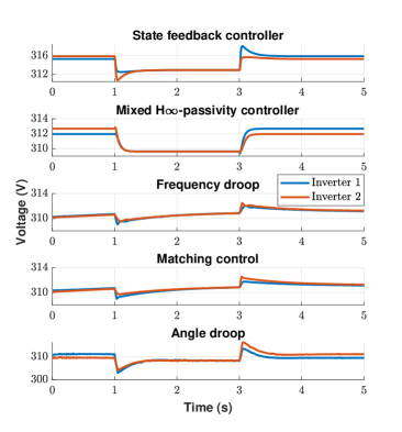
Fig. 7: System response to load change: voltage.

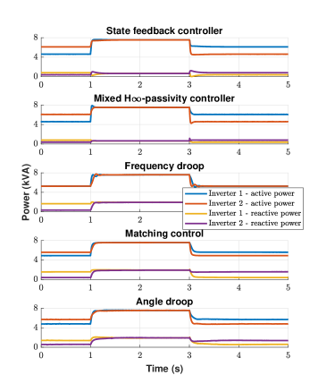
Fig. 8: System response to load change: power.

As discussed, one of the key advantages of the proposed control design framework is that plug-and-play operation is possible. We demonstrate this by simulating the plug-in of an additional inverter at bus 4 in the test network (Fig. 6). The response using the state feedback and the mixed $H_{\infty}$/passivity controllers is shown in Fig. 9, where this is also compared to traditional droop control. In the case of frequency droop, the phase angles of inverter 2 and 3 are synchronized exactly before connection, whereas in the proposed design no adjustment is necessary, and the inverters are unaware of the plug-in of another inverter. This is a challenging scenario that can lead to bad performance. As illustrated, plug-and-play operation is possible with the proposed controller and less severe oscillations are experienced than in the case of the traditional frequency droop controller.

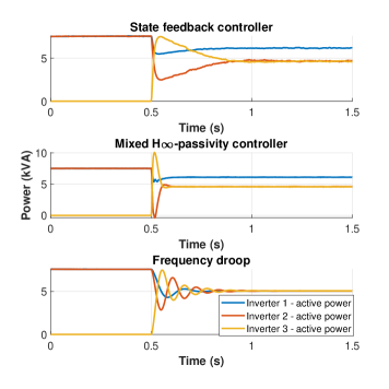
Fig. 9: Plug-and-play response.

V Conclusion

We have considered the problem of designing controllers for grid-forming converters in microgrids that regulate the voltage and frequency satisfactorily, achieve a power sharing property, and allow stability to be ensured via decentralized conditions. To this end, we propose a passivity-based controller design method for converter-based microgrids. Our proposed method achieves good performance while guaranteeing stability in a decentralized way via its passivity property. Furthermore, our controller improves the power sharing properties of the microgrid compared to previous non-droop approaches. Finally, realistic simulations are used to verify the performance of the proposed controllers. A comparative study and a demonstration of plug-and-play operation were included to show that the controller design improves the stability and dynamic response of the microgrid in response to both load and setpoint changes.

Appendix

In the appendices, we provide various definitions for the transmission line model as well as the proofs of all our results.

V-A Transmission line model

In this section we define the matrices $H$, $H_{B}$, $H_{C}$ that allow a concise representation of the line dynamics in (1). We start by defining various notions that are needed to specify these matrices.

• We consider a graph $(N_{L},E_{L})$ associated with the general RLC network representing the line dynamics in this case. In particular, we assign a node to each voltage in Fig. 1 (i.e. ($V^{i}_{dq}$, $V^{ij}_{dq,1}$, … $V^{ij}_{dq,n-1}$, $V^{j}_{dq}$)) and do this for all lines. There exists an edge between any two consecutive nodes along a line. Thus there is an edge associated with each current (($I^{ij}_{dq,1}$, $I^{ij}_{dq,2},...,I^{ij}_{dq,n-1}$) in Fig. 1) and this is true for all lines. $N_{L}$ is therefore the set of nodes $(1,2,\dots|N_{L}|)$ representing the voltages of the buses and internal capacitances, and $E_{L}\subset N_{L}\times N_{L}$ is the set of edges associated with the current of each line subsection. A direction is assigned to each edge in $E_{L}$ which can be arbitrarily chosen, and similarly the ordering of the edge in $E_{L}$ can be arbitrarily chosen. The nodes in the set $N_{L}$ are ordered such that a node $j\in N_{L},j\leq|N|$ corresponds to the bus $j\in N$.

• We enumerate the capacitances in the line model (for all lines), and the indices $(1,2,...,|N_{C}|)$ form the set $N_{C}$. The order of the enumeration corresponds to the order in $N_{L}$. To be precise, the node $i\in N_{L},i=|N|+j$ corresponds to the internal capacitance $j\in N_{C}$.

• $\mathcal{R}>0$, $\mathcal{L}>0$, $\mathcal{G}>0$, $\mathcal{C}>0$ are diagonal matrices of the equivalent line resistances, inductances, conductances, and capacitances respectively with respective dimensions $|E_{L}|\times|E_{L}|$, $|E_{L}|\times|E_{L}|$, $|N_{C}|\times|N_{C}|$, $|N_{C}|\times|N_{C}|$. The order of $\mathcal{R}$ and $\mathcal{L}$ corresponds to the order of the edges in $E_{L}$, and the order of $\mathcal{G}$ and $\mathcal{C}$ corresponds to the order of the nodes representing internal capacitances in $N_{C}$.

• $I^{\mathcal{N}}_{dq}$ is the vector of length $2|E_{L}|$ which represents the current (i.e. $I^{ij}_{dq,k}$ for all $(i,j)\in E$ and corresponding $k$) of every edge in $E_{L}$. This vector is ordered consistently with the order of the edges in $E_{L}$.

• $V^{C}_{dq}$ is a vector of length $2|N_{C}|$ which represents the voltages of the capacitors (i.e. $V^{ij}_{dq,k}$ for all $(i,j)\in E$ and corresponding $k$ in the line representation (1)), ordered correspondingly to the order in $N_{C}$.

We now define the matrices below with elements $0,1,-1$:

• $H$ is the $|N_{L}|\times|E_{L}|$ incidence matrix of the graph ($N_{L}$, $E_{L}$) which is defined as:
  $\begin{cases}H_{iz}=1&\text{if edge }z\text{ leaves node }i\in N_{L}\\ H_{iz}=-1&\text{if edge }z\text{ enters node }i\in N_{L}\\ H_{iz}=0&\text{otherwise}\end{cases}$
  i.e., $H$ illustrates for each edge in $E_{L}$ the nodes in $N_{L}$ it is connected to.

• $H_{B}$ is an $|N|\times|E_{L}|$ submatrix of $H$ that consists of the first $|N|$ rows of $H$; i.e., it illustrates the connection between edges/nodes for edges connected to buses in $N$.

• $H_{C}$ is an $|N_{C}|\times|E_{L}|$ submatrix of $H$ that consists of the last $|N_{C}|$ rows of $H$; i.e., it illustrates the connection between edges/nodes for edges connected to nodes associated with capacitances in $N_{C}$.

Hence, $H_{C}$ and $H_{B}$ are related to the incidence matrix $H$ by means of the equation $H=\begin{bmatrix}H_{B}^{T}&H_{C}^{T}\end{bmatrix}^{T}$.

V-B Proof of Proposition 1

This follows by using $\mathcal{V}_{\mathcal{N}}$ defined below to show that the condition for strict passivity stated in Definition 1 is satisfied.

$$\mathcal{V}_{\mathcal{N}}=\frac{1}{2} (V_{DQ}-V^{\ast}_{DQ})^{T}[\mathcal{L}\otimes I_{2}](I^{N}_{DQ}-I^{N\ast}_{DQ})\hskip 28.45274pt$$ (18)

$$+\frac{1}{2}(V^{C}_{DQ}-V^{C\ast}_{DQ})^{T}[\mathcal{C}\otimes I_{2}](V^{C}_{DQ}-V^{C\ast}_{DQ})$$

By taking the time derivative and substituting (2) we have

$$\dot{V}_{\mathcal{N}}= (V_{DQ}-V_{DQ}^{*})^{T}(I^{N}_{DQ}-I^{N*}_{DQ})$$ (19)

$$-(x_{\mathcal{N}}-x_{\mathcal{N}}^{*})^{T}{\small\begin{bmatrix}\mathcal{R}\otimes I_{2}&0\\ 0&\mathcal{G}\otimes I_{2}\end{bmatrix}}(x_{\mathcal{N}}-x_{\mathcal{N}}^{*})$$

where $x_{\mathcal{N}}=[(I^{N}_{DQ})^{T}\mbox{ }(V^{C}_{DQ})^{T}]^{T}$. The matrix ${\small\begin{bmatrix}\mathcal{R}\otimes I_{2}&0\\ 0&\mathcal{G}\otimes I_{2}\end{bmatrix}}$ is positive definite, which completes the proof.

V-C Proof of Theorem 1

The result in Proposition 1, together with equation (8), allows a straightforward LaSalle argument using the candidate Lyapunov function $\mathcal{V}(q)=\mathcal{V}_{\mathcal{N}}+\sum_{j=1}^{|N|}\mathcal{V}_{j}(x_{j})$, where $q=({\color[rgb]{0,0,0}x_{\mathcal{N}}},x_{1},x_{2},...,x_{|N|})$, $x_{\mathcal{N}}=[(I^{N}_{DQ})^{T}\mbox{ }(V^{C}_{DQ})^{T}]^{T}$, and $\mathcal{V}_{\mathcal{N}}$ as in (18) to prove asymptotic stability. Consider the time derivative of $\mathcal{V}(q)$. From (19), we have:

$$\dot{\mathcal{V}}_{\mathcal{N}}= -(x_{\mathcal{N}}-x_{\mathcal{N}}^{*})^{T}\begin{bmatrix}\mathcal{R}\otimes I_{2}&0\\ 0&\mathcal{G}\otimes I_{2}\end{bmatrix}(x_{\mathcal{N}}-x_{\mathcal{N}}^{*})$$

$$+(I_{DQ}-I^{\ast}_{DQ})^{T}(V_{DQ}-V^{\ast}_{DQ})$$

From Assumption 2 and Definition 1, we have the following for all buses $j\in N$: there exist open neighbourhoods $W_{j}$ of $i^{j*}_{DQ}$ and $X_{j}$ of $x_{j}^{*}$ such that $\dot{\mathcal{V}}_{j}(x_{j})\leq-(i^{j}_{DQ}-i^{j*}_{DQ})^{T}(v^{j}_{DQ}-v^{j*}_{DQ})$ for all ${\color[rgb]{0,0,0}i^{j}_{DQ}}\in W_{j}$ and $x_{j}\in X_{j}$. This implies that:

$$\sum_{j=1}^{|N|}\dot{\mathcal{V}}_{j}(x_{j})\leq -(I_{DQ}-I^{\ast}_{DQ})^{T}(V_{DQ}-V^{\ast}_{DQ})$$

Hence, we have:

$$\dot{\mathcal{V}}\leq-(x_{\mathcal{N}}-x_{\mathcal{N}}^{*})^{T}\begin{bmatrix}\mathcal{R}\otimes I_{2}&0\\ 0&\mathcal{G}\otimes I_{2}\end{bmatrix}(x_{\mathcal{N}}-x_{\mathcal{N}}^{*})$$ (20)

Each $\mathcal{V}_{j}(x_{j})$ has a strict local minimum at $x_{j}^{*}$, and $\mathcal{V}_{\mathcal{N}}$ is minimized at $(x_{\mathcal{N}}^{\ast})$. Thus $\mathcal{V}$ has a strict local minimum at the point $q^{*}:=({\color[rgb]{0,0,0}x_{\mathcal{N}}^{\ast}},x_{1}^{*},x_{2}^{*},...,x_{|N|}^{*})$. We then choose a neighbourhood about $q^{*}$ on which the following all hold:

1. $q^{*}$ is a strict minimum of $\mathcal{V}$.

2. $i^{j*}_{DQ}\in W_{j}$ and $x_{j}\in X_{j}$ for all $j\in N$.

3. $x_{j}\in X_{j}^{0}$ for all $j\in N$.

Thus from (20), $\mathcal{V}$ is nonincreasing with time and has a strict local minimum at $q^{*}$. Hence, for sufficiently small $\epsilon>0$ the level set $T=\{q:\mathcal{V}(q)-\mathcal{V}(q^{\ast})\leq\epsilon\}$ is compact and positively invariant with respect to the system (2)-(7). We then apply LaSalle’s Theorem [19] with function $\mathcal{V}$ on the compact positively invariant set $T$ as the Lyapunov-like function. This states that all solutions with initial conditions within $T$ converge to the largest invariant set $\Xi$ within $T$ that satisfies $\dot{\mathcal{V}}=0$. From (20) $\dot{\mathcal{V}}=0$ implies that $x_{\mathcal{N}}=x_{\mathcal{N}}^{\ast}$ and thus $I^{N}_{DQ}=I^{N\ast}_{DQ}$ and $V^{C}_{DQ}=V^{C\ast}_{DQ}$. The former further implies that $I_{DQ}=I^{*}_{DQ}$ from (2). Since the inputs to the bus dynamical systems $w_{j}^{*}=i^{j*}_{DQ}$ are constant within $\Xi$, we have that each trajectory in $\Xi$ converges to the equilibrium point $q^{\ast}$ as $t\to\infty$, as follows from the asymptotic stability of $x_{j}^{\ast}$ for constant $w_{j}=w_{j}^{\ast}$ (Assumption 2). Since $\mathcal{V}$ has a strict minimum at $q^{\ast}$ and is constant in $\Xi$ w.r.t. time, we have that $q(t)=q^{\ast}$ for all $t$ is the only trajectory in $\Xi$. Hence, all solutions with initial conditions within $T$ converge to the equilibrium point $q^{*}=({\color[rgb]{0,0,0}x_{\mathcal{N}}^{\ast}},x_{1}^{*},...,x_{|N|}^{*})$.

V-D Proof of Theorem 2

The dynamics considered (the state feedback controller $u=-K\tilde{x}-Mw$ in conjunction with the dynamics (6)) are linear. Hence without loss of generality (and for notational convenience) we can check the passivity property about the origin, since the passivity property of a linear system is not dependent on its equilibrium point. We will also neglect the bus index $j$ for simplicity, and use the following definitions as in (10): $A_{c}=\tilde{A}-\tilde{B}_{u}K$, $B_{c}=\tilde{B}_{w}-\tilde{B}_{u}M$, $C_{c}=\tilde{C}-\tilde{D}_{u}K$, and $D_{c}=\tilde{D}_{w}-\tilde{D}_{u}M$. Consider the storage function

$$\mathcal{V}=\frac{1}{2}\tilde{x}^{T}P\tilde{x}$$ (21)

in conjunction with the system (6) and $u=-K\tilde{x}-Mw$. To satisfy Assumption 2 with output-strict passivity index $\rho$, we require from (9) in Definition 1, $\dot{\mathcal{V}}\leq w^{T}z-\rho z^{T}z$. The RHS can be expanded as:

$$w^{T}z-\rho z^{T}z= \frac{1}{2}[w^{T}(C_{c}\tilde{x}+D_{c}w)+(C_{c}\tilde{x}+D_{c}w)^{T}w]-$$

$$-\rho[(C_{c}\tilde{x}+D_{c}w)^{T}(C_{c}\tilde{x}+D_{c}w)]$$ (22)

and $\dot{\mathcal{V}}$ is obtained by differentiating $\mathcal{V}$ along the trajectories of (6), noting that $u=-K\tilde{x}-Mw$:

$$\begin{split}&\dot{\mathcal{V}}=\frac{1}{2}[\dot{\tilde{x}}^{T}P\tilde{x}+\tilde{x}^{T}P\dot{\tilde{x}}]\\ &\leavevmode\nobreak\ \leavevmode\nobreak\ =\frac{1}{2}[(A_{c}\tilde{x}+B_{c}w)^{T}P\tilde{x}+\tilde{x}^{T}P(A_{c}\tilde{x}+B_{c}w)]\\ &\leavevmode\nobreak\ \leavevmode\nobreak\ =\frac{1}{2}[\tilde{x}^{T}(A_{c}^{T}P+PA_{c})\tilde{x}+\tilde{x}^{T}PB_{c}{\color[rgb]{0,0,0}w+w^{T}B_{c}}^{T}P\tilde{x}]\end{split}$$ (23)

We now recall the condition in Theorem 2 and the associated equation (10), and note that if (10) holds, so does:

$${\footnotesize\begin{bmatrix}\tilde{x}\\ w\end{bmatrix}^{T}\begin{bmatrix}A_{c}^{T}P+PA_{c}+2\rho C_{c}^{T}C_{c}&PB_{c}-C_{c}^{T}+2\rho C_{c}^{T}D_{c}\\ B_{c}^{T}P-C_{c}+2\rho D_{c}^{T}C_{c}&2\rho D_{c}^{T}D_{c}-D_{c}^{T}-D_{c}\end{bmatrix}\begin{bmatrix}\tilde{x}\\ w\end{bmatrix}\leq 0}$$ (24)

From  (22) and (23), $\dot{\mathcal{V}}\leq w^{T}z-\rho z^{T}z$ holds if (24) holds. Hence, satisfying Theorem 2 guarantees that the passivity condition in Assumption 2 is satisfied.

Regarding the asymptotic stability for constant input $w$ we consider the case $w=0$ without loss of generality (since the system is linear). We have in this case from the analysis above that $\dot{\mathcal{V}}\leq-\rho z^{T}z$. Asymptotic stability then follows from Lasalle’s Theorem with $\mathcal{V}$ as the Lyapunov function. In particular, $\dot{\mathcal{V}}=0$ implies $z=0$. From the system dynamics in (3) we have in this case $i_{iDQ}=0$ and from (5) $\zeta$ is constant. Since the Lyapunov function is radially unbounded an arbitrarily large compact invariant set can be constructed in which the largest invariant set for which $\dot{\mathcal{V}}=0$ is the equilibrium point, thus deducing asymptotic stability.

V-E LMI formulation of the $H_{\infty}$ and passivity conditions with dynamical controller

In this appendix, we present an LMI formulation for the problem of finding a controller such that we have output strict passivity of $T_{-{i}_{DQ}\rightarrow v_{DQ}}$ as in (9) together with the $H_{\infty}$ condition in (17).

As is commonly followed in $H_{\infty}$ control, to facilitate the control synthesis problem, we consider the block diagram in Fig. 10 which contains: the closed loop system $\mathcal{T}$ which has inputs and outputs associated with the transfer functions on which performance specifications are imposed, the controller $\mathcal{K}$ (given in (11)) and the generalized plant $\mathcal{P}$ (containing the inverter itself and the different weighting filters $W_{e}$, $W_{u}$ and $W_{d}$).

The different performance specifications (passivity and $H_{\infty}$) will be expressed using the performance input and output $w_{\text{perf}}=[(v_{DQ}^{ref})^{T}\leavevmode\nobreak\ -{i}_{DQ}^{T}]^{T}$ and $z_{\text{perf}}=[z_{e_{DQ}}^{T}\leavevmode\nobreak\ z_{u}^{T}\leavevmode\nobreak\ v_{DQ}^{T}]^{T}$. In particular,

• For passivity, the input and output signals are $w_{\text{pas}}=-{i}_{DQ}$ and $z_{\text{pas}}=v_{DQ}$.

• For $H_{\infty}$ constraints: the input and output signals are $w_{\infty}=[(v_{DQ}^{ref})^{T}\leavevmode\nobreak\ -{i}_{DQ}^{T}]^{T}$ and $z_{\infty}=[z_{e_{DQ}}^{T}\leavevmode\nobreak\ z_{u}^{T}]^{T}$

Fig. 10: Block diagram representing the $H_{\infty}$/passivity control synthesis problem. The inputs and outputs of the block $\mathcal{T}$ are associated with the transfer functions on which $H_{\infty}$/passivity conditions are imposed.

To formulate these performance specifications, a state space representation of the generalized plant $\mathcal{P}$ is required. We start with the weighting filters. As explained in Section IV-C, the weighting filters $W_{e}$, $W_{u}$ and $W_{d}$ are added to account for loop shaping constraints on $T_{v^{ref}_{DQ}\rightarrow e_{DQ}}$, $T_{v^{ref}_{DQ}\rightarrow u}$, $T_{-i_{DQ}\rightarrow v_{DQ}}$ and $T_{-i_{DQ}\rightarrow u}$. We denote $A_{W_{e}},B_{W_{e}},C_{W_{e}},D_{W_{e}}$ the matrices in the state space representation of $W_{e}$ (similarly for $W_{u}$ and $W_{d}$). The state vectors of $W_{e}$, $W_{u}$ and $W_{d}$ are denoted as $x_{W_{e}}$, $x_{W_{u}}$ and $x_{W_{d}}$ respectively. Their inputs are $(v^{ref}_{DQ}-v_{DQ})$, $u$ and $-i_{DQ}$ respectively while their outputs are denoted by $z_{e_{DQ}}$, $z_{u}$ and $\tilde{i}_{DQ}$ respectively (see Fig. 10).

Using $\mathcal{A}$, $\mathcal{B}_{u}$ and $\mathcal{B}_{w}$ given by (4), the generalized plant $\mathcal{P}$ has the following representation

$$\mathcal{P}:\leavevmode\nobreak\ \leavevmode\nobreak\ \leavevmode\nobreak\ \begin{bmatrix}\dot{\xi}\\ z_{\text{perf}}\\ y_{\text{control}}\end{bmatrix}=\begin{bmatrix}A_{\xi}&B_{1}&B\\ C_{1}&D_{11}&D_{12}\\ C&D_{21}&\bf{0}\\ \end{bmatrix}\begin{bmatrix}{\xi}\\ w_{\text{perf}}\\ u\end{bmatrix}$$ (25)

where ${\small\xi=[x^{T}\leavevmode\nobreak\ x_{W_{e}}^{T}\leavevmode\nobreak\ x_{W_{u}}^{T}\leavevmode\nobreak\ x_{W_{d}}^{T}]^{T}}$; ${\small w_{\text{perf}}=[(v_{DQ}^{ref})^{T}\leavevmode\nobreak\ -{i}_{DQ}^{T}]^{T}}$;
${\small z_{\text{perf}}=[z_{e_{DQ}}^{T}\leavevmode\nobreak\ z_{u}^{T}\leavevmode\nobreak\ v_{DQ}^{T}]^{T}}$; ${\small y_{\text{control}}=[(v^{ref}_{{DQ}})^{T}\leavevmode\nobreak\ \tilde{i}_{DQ}^{T}\leavevmode\nobreak\ i_{iDQ}^{T}\leavevmode\nobreak\ v_{DQ}^{T}]^{T}};$

$${\small\begin{split}&A_{\xi}=\begin{bmatrix}\leavevmode\nobreak\ \mathcal{A}&\bf{0}&\bf{0}&C_{W_{d}}\\ -[\bf{0}\leavevmode\nobreak\ \leavevmode\nobreak\ B_{W_{e}}]&A_{W_{e}}&\bf{0}&\bf{0}\\ \bf{0}&\bf{0}&A_{W_{u}}&\bf{0}\\ \bf{0}&\bf{0}&\bf{0}&A_{W_{d}}\end{bmatrix}\\ &B_{1}=\begin{bmatrix}\bf{0}&\mathcal{B}_{w}D_{W_{d}}\\ B_{W_{e}}&\bf{0}\\ \bf{0}&\bf{0}\\ \bf{0}&B_{W_{d}}\end{bmatrix}\leavevmode\nobreak\ \leavevmode\nobreak\ \leavevmode\nobreak\ \leavevmode\nobreak\ B=\begin{bmatrix}\mathcal{B}_{u}\\ \bf{0}\\ B_{W_{u}}\\ \bf{0}\end{bmatrix}\\ &C_{1}=\begin{bmatrix}-[\bf{0}\leavevmode\nobreak\ \leavevmode\nobreak\ D_{W_{e}}]&C_{W_{e}}&\bf{0}&\bf{0}\\ \bf{0}&\bf{0}&C_{W_{u}}&\bf{0}\end{bmatrix}\\ &C=\begin{bmatrix}I_{4}&\bf{0}&\bf{0}&\bf{0}\\ \bf{0}&\bf{0}&\bf{0}&\bf{0}\end{bmatrix}\\ &D_{11}=\begin{bmatrix}D_{W_{e}}&\bf{0}\\ \bf{0}&\bf{0}\end{bmatrix},D_{12}=\begin{bmatrix}\bf{0}\\ D_{W_{u}}\end{bmatrix},D_{21}=\begin{bmatrix}\bf{0}\\ I_{4}\end{bmatrix}\end{split}}$$ (26)

We are now able to present an LMI formulation for the problem of finding a controller $\mathcal{K}$ such that the required passivity and $H_{\infty}$ conditions are satisfied.

Theorem 3

Consider the dynamic feedback controller in (11) in conjunction with the dynamics (3).
The system  (3) with input $w$ and output $z$ satisfies 1) the passivity condition in Definition 1 referred to in Assumption 2 and is output-strictly passive with strictness index $\eta$ and 2) the $H_{\infty}$ condition in (17) if there exist $X$, $Y$, $\hat{A}$, $\hat{B}$, $\hat{C}$, and $\hat{D}$ such that the following LMIs hold

$${\small\begin{bmatrix}X&I\\ I&Y\end{bmatrix}>0}\leavevmode\nobreak\ \leavevmode\nobreak\ \leavevmode\nobreak\ \leavevmode\nobreak\ \leavevmode\nobreak\ \leavevmode\nobreak\ \leavevmode\nobreak\ \leavevmode\nobreak\ \leavevmode\nobreak\ \leavevmode\nobreak\ \leavevmode\nobreak\ \leavevmode\nobreak\ \leavevmode\nobreak\ \leavevmode\nobreak\ \leavevmode\nobreak\ \leavevmode\nobreak\ \leavevmode\nobreak\ \leavevmode\nobreak\ \leavevmode\nobreak\ \leavevmode\nobreak\ \leavevmode\nobreak\ \leavevmode\nobreak\ \leavevmode\nobreak\ \leavevmode\nobreak\ \leavevmode\nobreak\ \leavevmode\nobreak\ \leavevmode\nobreak\ \leavevmode\nobreak\ \leavevmode\nobreak\$$ (27)

$${\small\begin{bmatrix}M_{11}&M_{12}&M_{13_{\text{pas}}}&M_{14_{\text{pas}}}\\ M_{12}^{T}&M_{22}&M_{23_{\text{pas}}}&M_{24_{\text{pas}}}\\ M_{13_{\text{pas}}}^{T}&M_{23_{\text{pas}}}^{T}&M_{33_{\text{pas}}}&M_{34_{\text{pas}}}\\ M_{14_{\text{pas}}}^{T}&M_{24_{\text{pas}}}^{T}&M_{34_{\text{pas}}}^{T}&-\frac{1}{2}\eta^{-1}I\end{bmatrix}<0}$$ (28)

$${\small\begin{bmatrix}M_{11}&M_{12}&M_{13_{\infty}}&M_{14_{\infty}}\\ M_{12}^{T}&M_{22}&M_{23_{\infty}}&M_{24_{\infty}}\\ M_{13_{\infty}}^{T}&M_{23_{\infty}}^{T}&-I&M_{34_{\infty}}\\ M_{14_{\infty}}^{T}&M_{24_{\infty}}^{T}&M_{34_{\infty}}^{T}&-I\end{bmatrix}<0\leavevmode\nobreak\ \leavevmode\nobreak\ \leavevmode\nobreak\ }$$ (29)

with

$${\small\begin{split}&\leavevmode\nobreak\ \leavevmode\nobreak\ M_{11}=A_{\xi}X+XA_{\xi}^{T}+B\hat{C}+(B\hat{C})^{T}\\ &\leavevmode\nobreak\ \leavevmode\nobreak\ M_{12}=\hat{A}^{T}+(A_{\xi}+B\hat{D}C)\\ &\leavevmode\nobreak\ \leavevmode\nobreak\ M_{22}=A_{\xi}^{T}Y+YA_{\xi}+\hat{B}C+(\hat{B}C)^{T}\\ &\leavevmode\nobreak\ \leavevmode\nobreak\ M_{13_{\text{pas}}}=(B_{1}R_{\text{pas}}+B\hat{D}D_{21}R_{\text{pas}})-(L_{\text{pas}}C_{1}X+L_{\text{pas}}D_{12}\hat{C})^{T}\\ &\leavevmode\nobreak\ \leavevmode\nobreak\ M_{14_{\text{pas}}}=(L_{\text{pas}}C_{1}X+L_{\text{pas}}D_{12}\hat{C})^{T}\\ &\leavevmode\nobreak\ \leavevmode\nobreak\ M_{23_{\text{pas}}}=(YB_{1}R_{\text{pas}}+\hat{B}D_{21}R_{\text{pas}})-(L_{\text{pas}}C_{1}+L_{\text{pas}}D_{12}\hat{D}C)^{T}\\ &\leavevmode\nobreak\ \leavevmode\nobreak\ M_{24_{\text{pas}}}=(L_{\text{pas}}C_{1}+L_{\text{pas}}D_{12}\hat{D}C)^{T}\\ &\leavevmode\nobreak\ \leavevmode\nobreak\ M_{33_{\text{pas}}}=-(L_{\text{pas}}D_{11}R_{\text{pas}}+L_{\text{pas}}D_{12}\hat{D}D_{21}R_{\text{pas}})\\ &\leavevmode\nobreak\ \leavevmode\nobreak\ \leavevmode\nobreak\ \leavevmode\nobreak\ \leavevmode\nobreak\ \leavevmode\nobreak\ \leavevmode\nobreak\ \leavevmode\nobreak\ \leavevmode\nobreak\ \leavevmode\nobreak\ \leavevmode\nobreak\ \leavevmode\nobreak\ \leavevmode\nobreak\ \leavevmode\nobreak\ \leavevmode\nobreak\ \leavevmode\nobreak\ -(L_{\text{pas}}D_{11}R_{\text{pas}}+L_{\text{pas}}D_{12}\hat{D}D_{21}R_{\text{pas}})^{T}\\ &\leavevmode\nobreak\ \leavevmode\nobreak\ M_{34_{\text{pas}}}=(L_{\text{pas}}D_{11}R_{\text{pas}}+L_{\text{pas}}D_{12}\hat{D}D_{21}R_{\text{pas}})^{T}\\ &\leavevmode\nobreak\ \leavevmode\nobreak\ M_{13_{\infty}}=(B_{1}R_{\infty}+B\hat{D}D_{21}R_{\infty})\\ &\leavevmode\nobreak\ \leavevmode\nobreak\ M_{14_{\infty}}=(R_{\infty}C_{1}X+L_{\infty}D_{12}\hat{C})^{T}\\ &\leavevmode\nobreak\ \leavevmode\nobreak\ M_{23_{\infty}}=(YB_{1}R_{\infty}+\hat{B}D_{21}R_{\infty})\\ &\leavevmode\nobreak\ \leavevmode\nobreak\ M_{24_{\infty}}=(R_{\infty}C_{1}+L_{\infty}D_{12}\hat{D}C)^{T}\\ &\leavevmode\nobreak\ \leavevmode\nobreak\ M_{34_{\infty}}=(L_{\infty}D_{11}R_{\infty}+L_{\infty}D_{12}\hat{D}D_{21}R_{\infty})^{T}\\ \end{split}}$$

where $A_{\xi}$, $B$, $C$ $B_{1}$, $D_{11}$, $D_{12}$ and $D_{21}$ are given by (26) and

$$\begin{matrix}&L_{\text{pas}}&=&\begin{bmatrix}0_{2\times 4}&I_{2}\end{bmatrix}&R_{\text{pas}}&=&\begin{bmatrix}0_{2\times 2}&I_{2}\end{bmatrix}\\ &L_{\infty}&=&\begin{bmatrix}I_{4}&0_{4\times 2}\end{bmatrix}&R_{\infty}&=&I_{4}\end{matrix}$$ (30)

The controller $\mathcal{K}$ is constructed as

$${\small\begin{split}&{\color[rgb]{0,0,0}D_{K}=\hat{D},\qquad C_{K}=(\hat{C}-D_{K}CX)M^{-T}}{\color[rgb]{0,0,0},}\\ &B_{K}=N^{-1}(\hat{B}-YBD_{K}){\color[rgb]{0,0,0},}\\ &A_{K}=N^{-1}(\hat{A}-NB_{K}CX-YBC_{K}M^{T})M^{-T}\\ &\leavevmode\nobreak\ \leavevmode\nobreak\ \leavevmode\nobreak\ \leavevmode\nobreak\ \leavevmode\nobreak\ \leavevmode\nobreak\ \leavevmode\nobreak\ \leavevmode\nobreak\ \leavevmode\nobreak\ \leavevmode\nobreak\ \leavevmode\nobreak\ \leavevmode\nobreak\ \leavevmode\nobreak\ -N^{-1}Y(A+BD_{K}C)XM^{-T}\end{split}}$$ (31)

where $M$ and $N$ satisfy $MN^{T}=I-XY$ which can be solved through a singular value decomposition and Cholesky factorization.

Proof

Given the generalized plant dynamics (25) and the controller (11), we consider the closed-loop system

$$\begin{matrix}\mathcal{T}:\leavevmode\nobreak\ \leavevmode\nobreak\ \leavevmode\nobreak\ \begin{bmatrix}\dot{x}_{cl}\\ z_{\text{perf}}\end{bmatrix}=\begin{bmatrix}A_{c\ell}&B_{c\ell}\\ C_{c\ell}&D_{c\ell}\end{bmatrix}\begin{bmatrix}x_{c\ell}\\ w_{\text{perf}}\end{bmatrix}\end{matrix}$$

where ${x}_{cl}=\begin{bmatrix}\xi^{T}&x_{K}^{T}\end{bmatrix}^{T}$ and

$$A_{c\ell}=\begin{bmatrix}A_{\xi}+BD_{K}C&BC_{K}\\ B_{K}C&A_{K}\end{bmatrix} B_{c\ell}=\begin{bmatrix}B_{1}+BD_{K}D_{21}\\ B_{K}D_{21}\end{bmatrix}$$

$$C_{c\ell}=\begin{bmatrix}C_{1}+D_{12}D_{K}C&D_{12}C_{K}\end{bmatrix} D_{c\ell}=D_{11}+D_{12}D_{K}D_{21}$$

To formulate the passivity condition and the $H_{\infty}$ condition, we extract the corresponding closed-loop systems on which these conditions are imposed by selecting the appropriate input-output channels of $\mathcal{T}$ using $L_{\text{pas}}$, $R_{\text{pas}}$, $L_{\infty}$ and $R_{\infty}$ (given by (30)) as follows

$$\mathcal{T}_{\text{pas}}:{\small\begin{bmatrix}A_{\text{pas}}&B_{\text{pas}}\\ C_{\text{pas}}&D_{\text{pas}}\end{bmatrix}}={\small\begin{bmatrix}A_{c\ell}&B_{c\ell}R_{\text{pas}}\\ L_{\text{pas}}C_{c\ell}&L_{\text{pas}}D_{c\ell}R_{\text{ps}}\end{bmatrix}}\leavevmode\nobreak\ \leavevmode\nobreak\ \leavevmode\nobreak\ \leavevmode\nobreak\ \leavevmode\nobreak\ \leavevmode\nobreak\ \leavevmode\nobreak\ \leavevmode\nobreak\ \leavevmode\nobreak\ \leavevmode\nobreak\$$ (32)

$$\leavevmode\nobreak\ \leavevmode\nobreak\ \leavevmode\nobreak\ \leavevmode\nobreak\ \leavevmode\nobreak\ \leavevmode\nobreak\ \leavevmode\nobreak\ \mathcal{T}_{\infty}:{\small\begin{bmatrix}A_{\infty}&B_{\infty}\\ C_{\infty}&D_{\infty}\end{bmatrix}}={\small\begin{bmatrix}A_{c\ell}&B_{c\ell}R_{\infty}\\ L_{\infty}C_{c\ell}&L_{\infty}D_{c\ell}R_{\infty}\end{bmatrix}}$$ (33)

Using standard results from LQ control theory [29], the output-strict passivity of $\mathcal{T}_{\text{pas}}$ with passivity index $\eta$ is satisfied if and only if there exists $W_{\text{pas}}=W_{\text{pas}}^{T}>0$ such that

$${\small\begin{split}&\begin{bmatrix}A_{\text{pas}}^{T}W_{\text{pas}}+W_{\text{pas}}A_{\text{pas}}&W_{\text{pas}}B_{\text{pas}}-C_{\text{pas}}^{T}&C_{\text{pas}}^{T}\\ B_{\text{pas}}^{T}W_{\text{pas}}-C_{\text{pas}}&-D_{\text{pas}}^{T}-D_{\text{pas}}&D_{\text{pas}}^{T}\\ C_{\text{pas}}&D_{\text{pas}}&-\frac{\eta^{-1}}{2}I\end{bmatrix}<0\end{split}}$$ (34)

In the same way, the condition $\left\|\mathcal{T}_{\infty}\right\|_{\infty}\leq 1$ is satisfied if and only if there exists $W_{\infty}=W_{\infty}^{T}>0$ such that

$${\small\begin{split}&\begin{bmatrix}A_{\infty}^{T}W_{\infty}+W_{\infty}A_{\infty}&W_{\infty}B_{\infty}&C_{\infty}^{T}\\ B_{\infty}^{T}W_{\infty}&-I&D_{\infty}^{T}\\ C_{\infty}&D_{\infty}&-I\end{bmatrix}<0\leavevmode\nobreak\ \end{split}}$$ (35)

We use the results in [27] and [28, Chap 4] to formulate LMIs through which $A_{K}$, $B_{K}$, $C_{K}$ and $D_{K}$ can be found such that conditions (34)-(35) are satisfied.
In particular, let $W_{\infty}=W_{\text{pas}}=W$ and

$${\small W=\begin{bmatrix}Y&N\\ N^{T}&U\end{bmatrix},\leavevmode\nobreak\ \leavevmode\nobreak\ W^{-1}=\begin{bmatrix}X&M\\ M^{T}&V\end{bmatrix},\leavevmode\nobreak\ \leavevmode\nobreak\ \Phi=\begin{bmatrix}X&I\\ M^{T}&\bf{0}\end{bmatrix}}$$

where $X$, $Y$, $V$ and $U$ are symmetric matrices.
Due to $WW^{-1}=I$, we have $YX+NM^{T}=I$, $N^{T}X+UM^{T}=\bf{0}$, $YM+NV=\bf{0}$ and $UV-XY=\bf{0}$. Therefore, pre and post-multiplying of $W>0$ by $\Phi$ results in condition (27).
We define now the following change of variables

$${\small\begin{split}&\hat{A}=NA_{K}M^{T}+NB_{K}CX+YBC_{K}M^{T}+Y(A+BD_{K}C)X\\ &{\color[rgb]{0,0,0}\hat{B}=NB_{K}+YBD_{K},\quad\hat{C}=C_{K}M^{T}+D_{K}CX,\quad\hat{D}=D_{K}}\end{split}}$$ (36)

Conditions (28)-(29) are obtained by pre and postmultiplying conditions (34)-(35) (with ${\small W_{\infty}=W_{\text{pas}}=W}$) by ${\small\textbf{bdiag}(\Phi,I,I)}$ and using (36) to rewrite the obtained conditions, thus completing the proof.

References

- [1] F. Milano, et al, “Foundations and challenges of low-inertia systems” (Invited Paper), PSCC 2018, Dublin 2018, pp. 1-25.
- [2] M. C. Chandorkar, D. M. Divan and R. Adapa, “Control of parallel connected inverters in standalone AC supply systems,” in IEEE Trans. Ind. Appl., vol. 29, no. 1, pp. 136-143, Jan/Feb 1993.
- [3] W. Yao, M. Chen, J. Matas, J. M. Guerrero, and Z.-M. Qian, “Design and analysis of the droop control method for parallel inverters considering the impact of the complex impedance on the power sharing,” IEEE Trans. Ind. Electron., vol. 58, no. 2, pp. 576–588, Feb. 2011.
- [4] J. Watson, Y. Ojo, C. Spanias and I. Lestas, “Stability of power networks with grid-forming converters,” IEEE Powertech Milan, 2019.
- [5] R. Majumder, A. Ghosh, G. Ledwich and F. Zare, “Angle droop versus frequency droop in a voltage source converter based autonomous microgrid,” 2009 IEEE PES General Meeting, Calgary, AB, 2009, pp. 1-8.
- [6] Y. Sun, et al, “New perspectives on droop control in AC microgrid,” in IEEE Trans. Ind. Electron., vol. 64, no. 7, pp. 5741-5745, July 2017.
- [7] J. He, Y. Pan, B. Liang and C. Wang, “A Simple Decentralized Islanding Microgrid Power Sharing Method Without Using Droop Control,” in IEEE Trans. Smart Grid, vol. 9, no. 6, pp. 6128-6139.
- [8] M. S. Sadabadi, Q. Shafiee and A. Karimi, “Plug-and-Play Voltage Stabilization in Inverter-Interfaced Microgrids via a Robust Control Strategy,” IEEE Trans. Control Syst. Tech., vol. 25, no. 3, pp. 781-791, May 2017.
- [9] S. Derakhshan, M. Shafiee-Rad, Q. Shafiee and M. R. Jahed-Motlagh, “Decentralized Robust Voltage Control of Islanded AC Microgrids: An LMI-Based Approach,” 11th Power Electronics, Drive Systems, and Technologies Conference (PEDSTC), Tehran, Iran, 2020, pp. 1-6.
- [10] M. Babazadeh and H. Karimi, “A robust two-degree-of-freedom control strategy for an islanded microgrid,” IEEE Trans. Power Del., vol. 28, no. 3, pp. 1339–1347, Jul. 2013.
- [11] A. H. Etemadi, E. J. Davison, and R. Iravani, “A generalized decentralized robust control of islanded microgrids,” IEEE Trans. Power Syst., vol. 29, no. 6, pp. 3102–3113, Nov. 2014.
- [12] M. Tucci, G. Ferrari-Trecate, “A scalable, line-independent control design algorithm for voltage and frequency stabilization in AC islanded microgrids,” Automatica, vol. 111, 2020.
- [13] W. Du, R. H. Lasseter and A. S. Khalsa, “Survivability of Autonomous Microgrid During Overload Events,” in IEEE Trans. Smart Grid, vol. 10, no. 4, pp. 3515-3524, July 2019.
- [14] A. D. Paquette and D. M. Divan, “Virtual Impedance Current Limiting for Inverters in Microgrids With Synchronous Generators,” in IEEE Trans. Ind. Appl., vol. 51, no. 2, pp. 1630-1638, March-April 2015.
- [15] C. Spanias and I. Lestas, “A System Reference Frame Approach for Stability Analysis and Control of Power Grids,” in IEEE Trans. Power Syst., vol. 34, no. 2, pp. 1105-1115, March 2019.
- [16] L. Harnefors, X. Wang, A. G. Yepes and F. Blaabjerg, “Passivity-Based Stability Assessment of Grid-Connected VSCs - An Overview,” in IEEE Trans. Emerg. Sel. Topics Circuits Syst., vol. 4, no. 1, pp. 116-125, 2016.
- [17] C. Arghir, T. Jouini, F. Dörfler, “Grid-forming control for power converters based on matching of synchronous machines,” Automatica, vol. 95, pp. 273-282, 2018.
- [18] P. Nahata and G. Ferrari-Trecate, “Passivity-based Voltage and Frequency Stabilization in AC microgrids,” 2019 18th European Control Conference (ECC), Naples, Italy, 2019, pp. 1890-1895.
- [19] H. K. Khalil, Nonlinear Systems, 3rd edition, Prentice Hall, 2002.
- [20] F. Strehle, A. J. Malan, S. Krebs and S. Hohmann, “A Port-Hamiltonian Approach to Plug-and-Play Voltage and Frequency Control in Islanded Inverter-Based AC Microgrids,” 2019 IEEE 58th Conference on Decision and Control (CDC), Nice, France, 2019, pp. 4648-4655.
- [21] F. Strehle, A. J. Malan, S. Krebs and S. Hohmann, “Passivity Conditions for Plug-and-Play Operation of Nonlinear Static AC Loads”, IFAC-PapersOnLine, vol. 53, no. 2, 2020, pp. 12237-12243.
- [22] M. McCourt and P. Antsaklis, “Demonstrating passivity and dissipativity using computational methods”, Technical report, University of Notre Dame, August 2013.
- [23] A. van der Schaft, L2-Gain and Passivity Techniques in Nonlinear Control, Springer, 2016.
- [24] X. Wang, P. C. Loh and F. Blaabjerg, “Stability Analysis and Controller Synthesis for Single-Loop Voltage-Controlled VSIs,” in IEEE Trans. Power Elec., vol. 32, no. 9, pp. 7394-7404, Sept. 2017.
- [25] T. Qoria et al., “Tuning of AC voltage-controlled VSC based Linear Quadratic Regulation,” IEEE PowerTech, Milan, Italy, 2019, pp. 1-6.
- [26] P. Apkarian, P. Gahinet, and C. Buhr, “Multi-model, multi-objective tuning of fixed-structure controllers,” European Control Conf. (ECC), Strasbourg, June 2014.
- [27] C. Scherer, P. Gahinet and M. Chilali, “Multiobjective output-feedback control via LMI optimization,” in IEEE Trans. Auto. Control, vol. 42, no. 7, pp. 896-911, July 1997.
- [28] C. Scherer, and S. Weiland, “Linear Matrix Inequalities in Control,” in Dutch Institute for Systems and Control (DISC), 2005.
- [29] J. C. Willems, “Least-squares stationary optimal control and the algebraic Riccati equation,” in IEEE Trans. Auto. Control, vol. 16, no. 6, pp. 621-634, 1971.