Low-frequency vibrational spectrum of mean-field disordered systems

Abstract

We study a recently introduced and exactly solvable mean-field model for the density of vibrational states ${\cal D}(\omega)$ of a structurally disordered system. The model is formulated as a collection of disordered anharmonic oscillators, with random stiffness $\kappa$ drawn from a distribution $p(\kappa)$, subjected to a constant field $h$ and interacting bilinearly with a coupling of strength $J$. We investigate the vibrational properties of its ground state at zero temperature. When $p(\kappa)$ is gapped, the emergent ${\cal D}(\omega)$ is also gapped, for small $J$. Upon increasing $J$, the gap vanishes on a critical line in the $(h,J)$ phase diagram, whereupon replica symmetry is broken. At small $h$, the form of this pseudogap is quadratic, ${\cal D}(\omega)\sim\omega^{2}$, and its modes are delocalized, as expected from previously investigated mean-field spin glass models. However, we determine that for large enough $h$, a quartic pseudogap ${\cal D}(\omega)\sim\omega^{4}$, populated by localized modes, emerges, the two regimes being separated by a special point on the critical line. We thus uncover that mean-field disordered systems can generically display both a quadratic-delocalized and a quartic-localized spectrum at the glass transition.

Introduction —

The vibrational spectrum of structural glasses displays a series of universal features in different frequency ranges, which are responsible for important material properties, such as wave attenuation, heat transport, and plasticity Ruocco and Sette (2001); Nakayama (2002); Buchenau et al. (1991). Motivated by these observations, several authors have constructed simple models of the non-phononic vibrational density of states of structurally disordered systems, ${\cal D}(\omega)$ Kühn and Horstmann (1997); Gurarie and Chalker (2003a); Gurevich et al. (2003); Grigera et al. (2003); Parshin et al. (2007); DeGiuli et al. (2014); Franz et al. (2015); Baity-Jesi et al. (2015); Sharma et al. (2016); Benetti et al. (2018); Fyodorov and Le Doussal (2018); Stanifer et al. (2018); Ikeda (2019); Baggioli and Zaccone (2019); Shimada et al. (2020a); Fyodorov and Le Doussal (2020); Das et al. (2020). Mean-field models typically display a quadratic spectrum, ${\cal D}(\omega)\sim\omega^{2}$ Franz et al. (2015); Sharma et al. (2016), of delocalized and featureless modes Livan et al. (2018); this delocalization is inherently different from the one associated with phononic excitations in solids (which are absent in the mean-field limit), and is a manifestation of the marginal stability associated to replica symmetry breaking Mezard et al. (1987); Parisi et al. (2020).

On the contrary, numerical simulations of model glass formers in finite dimension have revealed that non-phononic excitations in those systems are quasi-localized in nature, that they emerge from self-organized glassy frustration, and that they follow a seemingly universal quartic law ${\cal D}(\omega)\sim\omega^{4}$ Laird and Schober (1991); Lerner et al. (2016); Mizuno et al. (2017); Kapteijns et al. (2018); Wang et al. (2019); Richard et al. (2020). Given these discrepancies with the mean-field scenario detailed above, and the localized nature of these excitations, the naive expectation is that the modes that populate the quartic law would disappear in the mean-field limit, and that mean-field models are therefore unable to tell much about the physics responsible for the $\omega^{4}$ spectrum of structural glasses Charbonneau et al. (2016); Ikeda and Shimada (2019); Shimada et al. (2020b).

Nearly two decades ago, Gurevich, Parshin and Schober (GPS) proposed a three-dimensional lattice model Gurevich et al. (2003) for this glassy density of states, formulated in terms of interacting anharmonic oscillators, with a coupling strength that decays with distance as $\sim\!r^{-3}$, where $r$ is the distance between the oscillators. GPS showed numerically that ${\cal D}(\omega)\!\sim\!\omega^{4}$ emerges in that model, and proposed a phenomenological theory Gurevich et al. (2003); Parshin et al. (2007), which has later been investigated by other authors Das et al. (2020). A similar mean-field model was studied by Kühn and Horstmann (KH) Kühn and Horstmann (1997), who however did not investigate the vibrational spectrum; as we will show below, their model’s spectrum follows ${\cal D}(\omega)\!\sim\!\omega^{2}$.

In this Letter, we study a recently introduced model Rainone et al. (2020), which corresponds to both the infinite-dimensional, mean-field version of the GPS model, and to a generalization of the KH model. Following Ref. Rainone et al. (2020), we hereafter refer to it as the KHGPS model. The model is formulated as a collection of $N$ interacting anharmonic oscillators, each represented by a generalized coordinate $x_{i}$ and stiffness $\kappa_{i}$ ; the model’s Hamiltonian reads

$$H\equiv\sum_{i<j}J_{ij}x_{i}x_{j}+\frac{1}{2}\sum_{i}\kappa_{i}x_{i}^{2}+\frac{1}{4!}\sum_{i}x_{i}^{4}-h\sum_{i}x_{i}\,.$$ (1)

Here the interactions $J_{ij}$ are assumed to be Gaussian, i.i.d. random couplings of variance $J^{2}/N$ $\forall\ i\!\neq\!j$, and $J$ represents the strength of the disordered interactions, taken to be space-independent. The harmonic stiffnesses $\kappa_{i}$ are characterized by a distribution $p(\kappa)$ which we take as uniform in $[\kappa_{m},\kappa_{{}_{\!M}}]$ with $\kappa_{{}_{\!M}}\geq\kappa_{m}\geq 0$, in such a way that all the oscillators have a single minimum at $J=0$. An external constant “magnetic” field $h$ is added in order to break the spurious $x_{i}\to-x_{i}$ symmetry that has no counterpart in amorphous solids Urbani and Biroli (2015); Albert et al. (2020). The model is related to a soft-spin version of the Sherrington-Kirkpatrick model Sompolinsky and Zippelius (1982).

In what follows we describe the exact solution of the KHGPS model using the replica method Kühn and Horstmann (1997); Mezard et al. (1987). We construct the phase diagram of the model, in the plane of the applied magnetic field $h$ and the coupling strength $J$. We rigorously show that, for $\kappa_{m}>0$, the model’s spectrum is gapped at small enough coupling, in the replica symmetric phase where the energy landscape is convex. Upon increasing the coupling strength, a phase transition is encountered, whereupon replica symmetry is broken, the energy landscape becomes rough, and the gap in the spectrum closes. On this critical line, the spectrum behaves as ${\cal D}(\omega)\sim\omega^{2}$ at small $h$, a typical mean-field scenario. Conversely, for large $h$, the spectrum behaves as ${\cal D}(\omega)\sim\omega^{4}$ and its modes are partially localized. The two regimes are separated by a special point on the critical line, whose location is determined. All in all, our work demonstrates that disordered mean-field models can display a quartic density of states of localized modes in certain regions of their phase diagram, including critical lines whereupon replica symmetry is broken. Related results have been reported in Ref. Lupo (2017) for the XY model defined on a random graph, which is however much more difficult to analyze. This result opens new perspectives for the microscopic understanding of the universal ${\cal D}(\omega)\sim\omega^{4}$ law in finite-dimensional glassy systems. Furthermore, it shows that replica symmetry breaking (RSB) phase transitions can present profoundly different characteristics from the marginal stability scenario usually associated to it, even at a mean-field level.

Vibrational spectrum —

The Hessian ${\cal M}_{ij}\!\equiv\!\partial^{2}H/\partial x_{i}\partial x_{j}$ corresponding to $H$ takes the form

$$\mathcal{M}_{ij}=J_{ij}+\delta_{ij}\left(\kappa_{i}+\frac{1}{2}x^{2}_{i}\right)\equiv J_{ij}+\delta_{ij}a_{i}\,,$$ (2)

which is the sum of a member ($J_{ij}$) of the Gaussian Orthogonal ensemble (GOE) of random matrices Livan et al. (2018) and of a diagonal matrix $A_{ij}=a_{i}\delta_{ij}$, with diagonal elements $a_{i}\equiv\kappa_{i}+x_{i}^{2}/2$. Assuming that there is no statistical correlation between these two matrices, calculating the spectrum of their sum becomes a standard problem in random matrix theory Livan et al. (2018), which only requires knowledge of the statistics of the diagonal part. Past efforts in calculating typical ground-state spectra of mean-field disordered systems Franz et al. (2015) indicate that this assumption is valid, hence we adopt it here and proceed as follows.

Assuming that the statistics $p(a)$ of the diagonal elements is known and has support in $[a_{m},a_{{}_{\!M}}]$ (we will compute it below), one can compute the density of eigenvalues $\rho_{{}_{\!\mathcal{M}}}(\lambda)$ of ${\cal M}$ by defining the resolvent Bun et al. (2017),

$$\mathfrak{g}_{{}_{\!\mathcal{M}}}(z)\equiv\int\differential\lambda\ \frac{\rho_{{}_{\!\mathcal{M}}}(\lambda)}{z-\lambda}\,,$$ (3)

which implies

$$\rho_{{}_{\!\mathcal{M}}}(\lambda)=\frac{1}{\pi}\lim_{\eta\to 0^{+}}{\rm Im}\,[\mathfrak{g}_{{}_{\!\mathcal{M}}}(\lambda-i\eta)]\,.$$ (4)

The resolvent of ${\cal M}$ is then implicitly expressed in terms of the spectrum of the diagonal part, ${\rho_{{}_{\!A}}(a)=p(a)}$, as Bun et al. (2017)

$$\mathfrak{g}_{{}_{\!\mathcal{M}}}(z)=\int_{a_{m}}^{a_{{}_{\!M}}}\differential a\,p(a)\frac{1}{z-a-J^{2}\mathfrak{g}_{{}_{\!\mathcal{M}}}(z)}\,.$$ (5)

This equation requires a numerical solution, but the position and shape of the lower edge of the spectrum can be worked out analytically. Let us define ${g(z)\!\equiv\!\mathfrak{g}_{{}_{\!\mathcal{M}}}(z)\!-\!z/J^{2}}$; one can then recast Eq. (5) as

$$z=-J^{2}\int_{a_{m}}^{a_{{}_{\!M}}}\differential a\,p(a)\left[g+\frac{1}{a+J^{2}g}\right]\equiv{\cal F}(g)\,.$$ (6)

We next argue as follows: for $\lambda$ outside of the support of the spectrum $\rho_{{}_{\!\mathcal{M}}}(\lambda)$ and in the limit $\eta\!\to\!0$, Eq. (4) implies that $g(z)$ cannot have an imaginary part. We therefore expect a band of values of the function ${\cal F}(g)$ to be forbidden for real $g$, and to correspond to the support of the spectrum. Let us then consider which values ${\cal F}(g)$ can attain for real $g$. This function is obviously not defined to the left of $-a_{{}_{\!M}}/J^{2}$ or to the right of $-a_{m}/J^{2}$, and intuitively, we expect the branch for $g\!>\!-a_{m}/J^{2}$ to be the one controlling the lower edge; therefore, this branch needs to be bounded from above. There are then only two possibilities: (i) The function ${\cal F}(g)$ has a maximum $g_{m}$ for $g\!>\!-a_{m}/J^{2}$, meaning that ${\cal F}^{\prime}(g_{m})\!=\!0$. The corresponding value of ${\cal F}$, $\lambda_{m}\!=\!{\cal F}(g_{m})$, is then the lower edge of the spectrum. In this case, the support of the diagonal elements has no influence on the lower edge, and the GOE part of ${\cal M}$ dominates: close to the edge the eigenvectors are delocalized and $\rho_{{}_{\!\mathcal{M}}}(\lambda)\!\propto\!(\lambda\!-\!\lambda_{m})^{1/2}$ Lee and Schnelli (2016). We dub this a GOE-like spectrum. (ii) The function ${\cal F}(g)$ has no maximum for $g\!>\!-a_{m}/J^{2}$. In this case, the value of $g$ that corresponds to the edge must be $g_{m}\!=\!-a_{m}/J^{2}$, and the lower edge itself is

$$\lambda_{m}={\cal F}\left(-\frac{a_{m}}{J^{2}}\right)=a_{m}-J^{2}\int_{a_{m}}^{a_{{}_{\!M}}}\differential a\,p(a)\frac{1}{a-a_{m}}\ .$$ (7)

The edge is then determined by the support of $p(a)$, and dominated by the diagonal part of ${\cal M}$, and the eigenvectors near the edge are partially localized Lee and Schnelli (2016). We dub this a DIAG-like spectrum. Furthermore, if $p(a)\sim(a-a_{m})^{\nu}$ near its lower edge, one can show by an expansion near $g_{m}$ that $\rho_{{}_{\!\mathcal{M}}}(\lambda)\sim(\lambda-\lambda_{m})^{\nu}$.

The value of coupling that separates the two regimes is such that ${\cal F}^{\prime}(g=g_{m})=0$, which gives the self-consistent equation:

$$\Lambda=1-J^{2}\int_{a_{m}}^{a_{{}_{\!M}}}\differential a\,p(a)\frac{1}{(a-a_{m})^{2}}=0\ ,$$ (8)

such that $\Lambda>0$ corresponds to a DIAG-like and $\Lambda<0$ corresponds to a GOE-like spectrum. Note that because $p(a)$ and its edges depend on $J$, this equation defines the critical value of coupling at which the spectrum changes shape only implicitly.

Replica method —

We next aim at determining the statistics $p(a)$ of the diagonal elements $a_{i}$ appearing in Eq. (2), which depend on the oscillator positions $x_{i}$ in the ground state of the model, and can be determined by solving its thermodynamics in the zero-temperature (${T\!\to\!0}$) limit. We do so by employing the replica method Mezard et al. (1987); we assume that the ground state is unique, which corresponds to a replica-symmetric (RS) ansatz. This picture is expected to be justified as long as the coupling strength $J$ is below a critical threshold $J_{c}(h)$, which we self-consistently determine below.

We briefly delineate the steps in obtaining the RS solution of the model, leaving the details to Appendix B. The mean-field nature of the model allows one to write its solution as a problem of decoupled oscillators in an effective, self-consistent random external potential, which in the $T\!\to\!0$ limit takes the form

$$v_{\rm eff}(x)\equiv\frac{x^{4}}{4!}+\frac{m}{2}x^{2}-(f+h)x\ ,\quad m=\kappa-J^{2}\chi\ ,$$ (9)

where $f$ is a Gaussian random force of zero mean and variance $J^{2}\tilde{q}$, and the new parameters $\chi$ and $\tilde{q}$ emerge from the correlations between different replicas generated by the disorder, and have to be determined self-consistently Mezard et al. (1987).

Depending on the value of the coefficients, the effective potential can be either an asymmetric single well (SW) or double well (DW), with two minima separated by an energy barrier. In particular, if the effective stiffness $m$ is negative, there is always some value of the field $f$ for which the potential is a DW. We thus conclude that if ${m_{m}=\kappa_{m}-J^{2}\chi<0}$, DWs appear with finite probability, and we show in Appendix B.4 that in this case the RS solution is always unstable towards RSB. Consequently, we now restrict ourselves to the case $m_{m}\geq 0$, which is realized at small enough $J$ if $\kappa_{m}>0$, and we discuss the RS phase of the model.

Under the assumption $m_{m}\geq 0$, we show in the Appendix that the parameters $\tilde{q}$ and $\chi$ are self-consistently determined through the equations

$$\chi=\left\langle\frac{1}{v_{\rm eff}^{\prime\prime}(x^{*}(f,m))}\right\rangle_{m,f}\ ,\quad\tilde{q}=\langle\left(x^{*}(f,m)\right)^{2}\rangle_{m,f}\ ,$$ (10)

where $x^{*}(f,m)$ denotes the point of absolute minimum of the effective potential, and the average is taken over the random effective stiffnesses $m\,$$\,\sim\,$$\,U(m_{m}$$=$$\kappa_{m}$$-$$J^{2}\chi,\,$$m_{{}_{\!M}}$$=$$\kappa_{{}_{\!M}}$$-$$J^{2}\chi)$ and random fields ${f\sim{\cal N}(0,J^{2}\tilde{q})}$. The self-consistency of this picture is tested by verifying the positivity of the replicon eigenvalue $\lambda_{R}$ of the Hessian matrix of the replica action Mezard et al. (1987); Parisi et al. (2020). The definition of the replica action and the computation of the replicon can be found in Appendix B.3. The final result reads

$$\lambda_{R}=1-J^{2}\left\langle\frac{1}{v_{\rm eff}^{\prime\prime}(x^{*}(f,m))^{2}}\right\rangle_{m,f}\ .$$ (11)

Recalling that ${a=\kappa+x^{2}/2=v_{\rm eff}^{\prime\prime}(x)+J^{2}\chi}$, cf. Eq. (2), where $x$ has to be evaluated in $x^{*}(f,m)$, we can express $\chi$ and $\lambda_{R}$ as

$$\begin{split}\chi&=\int_{a_{m}}^{a_{{}_{\!M}}}\differential a\,p(a)\frac{1}{a-J^{2}\chi}\ ,\\ \lambda_{R}&=1-J^{2}\int_{a_{m}}^{a_{{}_{\!M}}}\differential a\,p(a)\frac{1}{(a-J^{2}\chi)^{2}}\ ,\end{split}$$ (12)

where $\lambda_{R}$ differs from $\Lambda$ in Eq. (8) by the replacement of $a_{m}$ by $J^{2}\chi$ in the denominator of the integrand. Note that ${a=m+J^{2}\chi+x^{2}/2}$, hence under the assumption that $m_{m}\geq 0$, we have ${a_{m}\geq J^{2}\chi}$, which imples $\lambda_{R}\geq\Lambda$.

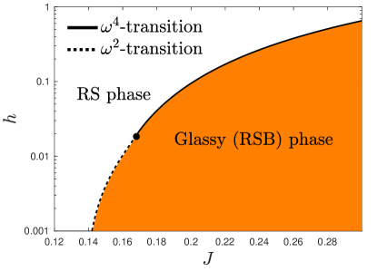
Figure 1: Phase diagram of the model for $\kappa_{m}=0.1$ and $\kappa_{{}_{\!M}}=1$ in the $(h,J)$ plane. The line $J_{c}(h)$ separates the convex-landscape RS phase from the rough-landscape RSB phase. Along the dotted line, $\mathcal{D}(\omega)\propto\omega^{2}$ at the transition, whilst $\mathcal{D}(\omega)\propto\omega^{4}$ on the solid line.

Phase diagram —

We are now in a position to determine the phase diagram of the model in the $(h,J)$ plane. We fix here $\kappa_{m}=0.1$ and $\kappa_{{}_{\!M}}=1$, but the qualitative picture is independent of this choice as long as $\kappa_{m}>0$. At $J=0$, the curvatures $v_{\rm eff}^{\prime\prime}(x^{*})$ are finite and consequently $\chi$ is finite. Hence, at $J=0$ we have $m=\kappa$ and consequently for small enough $J$, the condition $m_{m}>0$ is satisfied. Because $m_{m}>0$, we have $a_{m}>J^{2}\chi$ and the integral that appears in Eq. (12) is finite, leading to $\lambda_{R}\approx 1$ for $J\approx 0$. We thus conclude that the RS phase is stable at small $J$. While it is easy to show that the spectrum is always gapped in this phase, the sign of $\Lambda$, and thus the shape of the spectrum near its edge, depends on the behavior of $p(a)$ near $a_{m}$ and on the values of $a_{m}$ and $a_{{}_{\!M}}$. For example, the KH model studied in Ref. Kühn and Horstmann (1997) has $\kappa_{m}=\kappa_{{}_{\!M}}=1$ and in that case $a_{m}=a_{{}_{\!M}}$ leading formally to $\Lambda=-\infty$, in such a way that the spectrum is always GOE-like. With our choice of $p(\kappa)$, instead, the integral in Eq. (8) is finite and the spectrum is always DIAG-like at low enough $J$.

The RS phase can then become unstable in two ways: (i) The replicon can vanish, while $m_{m}$ remains strictly positive. In this case, at the transition point we have $\Lambda\leq\lambda_{R}=0$, hence the spectrum is GOE-like. For a GOE-like spectrum to be gapless, the two equations $\lambda_{m}$$=$${\cal F}(g_{m})$$=$$0$ and ${\cal F}^{\prime}(g_{m})$$=$$0$ must hold, which is equivalent to Eqs. (12) with $\lambda_{R}$$=$$0$ and $g_{m}$$=$$-\chi$. Hence, the spectrum is gapless at the critical point and $\rho_{{}_{\!\mathcal{M}}}(\lambda)\sim\lambda^{1/2}$, which is equivalent to ${\cal D}(\omega)\sim\omega^{2}$. Just above the critical point, the replicon becomes negative. This is a standard RSB transition, observed in several spin glass models. (ii) The lower bound of the effective stiffness can vanish, $m_{m}=0$, while the replicon is still positive, $\lambda_{R}>0$. When $m_{m}<0$, there is a finite probability of having DWs in the ensemble of effective potentials, and we show in Appendix B.4 that this formally implies $\lambda_{R}=-\infty$. Hence, the replicon jumps discontinuously to minus infinity beyond this transition. At the transition point, $m_{m}=0$ implies (see Appendix C.2 for details) that $a_{m}=J^{2}\chi$, which implies that $\Lambda=\lambda_{R}>0$ and the spectrum is DIAG-like. Furthermore, close to its lower edge,

$$p(a)\sim(a-J^{2}\chi)^{3/2}\qquad\Longrightarrow\qquad p(\tilde{a})\sim\tilde{a}^{3/2}\ ,$$ (13)

where $\tilde{a}=v_{\rm eff}^{\prime\prime}(x^{*})=a-J^{2}\chi$ is the curvature of the effective potential at its minimum. Note that Eq. (10) then gives $\chi=\langle 1/\tilde{a}\rangle$ and from Eq. (7) it follows that $\lambda_{m}=J^{2}[\chi-\langle 1/\tilde{a}\rangle]=0$. We conclude that the spectrum is gapless and DIAG-like, i.e. $\rho_{{}_{\!\mathcal{M}}}(\lambda)\sim\lambda^{3/2}$, or equivalently ${\cal D}(\omega)\sim\omega^{4}$.

The phase diagram obtained by solving numerically Eqs. (10) is reported in Fig. 1. We observe that the glass transition line $J_{c}(h)$ falls into case (i) for small $h$, and into case (ii) for large $h$. The two lines are separated by a special point at which $m_{m}=0$ and $\lambda_{R}=0$ simultaneously. We also verify these predictions numerically, by directly calculating the spectrum $\mathcal{D}(\omega)$ of the Hessian in the minima of the Hamiltonian in Eq. (1), obtained by means of a gradient descent algorithm . These numerical results, which confirm our theoretical predictions, are reported in Fig. 2. We note that when $\kappa_{m}$ is reduced and approaches zero, the line $J_{c}(h)$ moves towards the left, i.e. towards smaller values of $J$, and the $\omega^{4}$ region increases; when $\kappa_{m}=0$, the model is in the RSB phase at all $J$. This regime was studied numerically and through a scaling theory in Ref. Rainone et al. (2020).

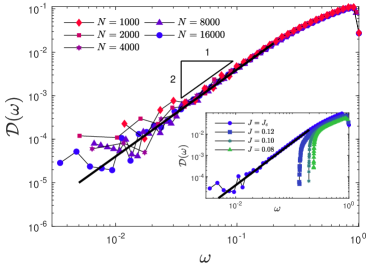
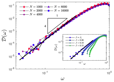
Figure 2: Numerical results for the vibrational spectrum of the model, at two selected values of $h$ (top: $h=0$, ${J_{c}(h)=0.137138}$ and bottom: $h=0.157220$, $J_{c}(h)=0.218$) corresponding to the two possible shapes of the spectrum. At the transition, we show multiple system sizes to confirm the gaplessness of the spectrum (main panels). The gap in the spectrum closes as the critical line is approached from the RS phase by increasing the coupling (insets).

Discussion —

We studied a mean-field model of interacting disordered anharmonic oscillators Rainone et al. (2020) having, in absence of coupling, a gapped spectrum. We showed that at small coupling the spectrum remains gapped Ji et al. (2020), and that at the glass transition point it can display either the universal ${{\cal D}(\omega)\!\sim\!\omega^{4}}$ localized spectra observed in finite-dimensional computer glass models Baity-Jesi et al. (2015); Lerner et al. (2016); Kapteijns et al. (2018); Richard et al. (2020); Wang et al. (2019); Mizuno et al. (2017) and in the random graph XY model Lupo (2017), or the standard ${{\cal D}(\omega)\!\sim\!\omega^{2}}$ observed in most mean-field spin glass models and jammed sphere packings Sharma et al. (2016); Charbonneau et al. (2016); DeGiuli et al. (2014); Franz et al. (2015). The immediate implication of our results is that systems at a RSB transition, and possibly even deep within the RSB phase, can in fact exhibit localized excitations, even at the mean-field level. The class of models to which the KHGPS model studied here belongs is expected to be rather broad — according to existing evidence Gurevich et al. (2003); Das et al. (2020); Gurarie and Chalker (2003a) — and largely robust to changes in these models’ input.

We note that an effective potential in the form of a quartic polynomial, Eq. (9), naturally emerges from our theory. This effective potential, which resembles the Soft Potential Model framework Buchenau et al. (1991, 1992); Gurarie and Chalker (2003b) that also predicts a $\omega^{4}$ nonphononic spectrum under some nontrivial assumptions (spelled out, e.g., in Gurarie and Chalker (2003a)). In light of our results, the Soft Potential Model can be viewed as an effective description of the collective, many-body statistical-mechanics of the KHGPS model.

Moreover, we note that the zero temperature limit of the spin glass susceptibility behaves very differently on the two parts of the critical line, being divergent when the spectrum at the transition is $\omega^{2}$, and finite when the spectrum is $\omega^{4}$ . Finally, we stress that our results apply upon approaching the transition at strictly zero temperature, and therefore it is important to investigate the model’s behavior at finite temperature.

In this work, we limited ourselves to the investigation of the RS phase of the model with $\kappa_{m}>0$, up to the critical line whereupon replica symmetry is broken and a glassy phase appears. A natural direction for future research is to investigate the vibrational spectrum deep in the glass phase. One might expect, by continuity arguments, that the quartic spectrum extends into the glass phase, hence being valid in a finite region of the phase diagram. This point of view seems to be supported by the numerical results of Ref. Rainone et al. (2020), but whether this intuition is correct can only be confirmed by an investigation of the RSB equations of the model. The gradient descent dynamics might also display interesting features in the glass phase Cugliandolo and Kurchan (1993); Folena et al. (2020) and, if minima reached by quenching dynamics retain the properties of the model at the transition, one could expect different (or even the absence of) aging dynamics.

Acknowledgements.—We benefited from discussions with Giulio Biroli, Jean-Philippe Bouchaud, Gustavo Düring, Eric De Giuli, and Guilhem Semerjian. This project has received funding from the European Research Council (ERC) under the European Union’s Horizon 2020 research and innovation programme (grant agreement n° 723955 - GlassUniversality) and by a grant from the Simons Foundation (#454955, Francesco Zamponi). P. U. acknowledges support by ”Investissements d’Avenir” LabEx-PALM (ANR-10-LABX-0039-PALM). E. B. acknowledges support from the Minerva Foundation with funding from the Federal German Ministry for Education and Research, the Ben May Center for Chemical Theory and Computation, and the Harold Perlman Family. E. L. acknowledges support from the NWO (Vidi grant no. 680-47-554/3259).

Appendix A The spectrum

The Hessian matrix, evaluated in a minimum $x^{*}_{i}$ of the Hamiltonian, is the sum of a GOE matrix $J_{ij}$ and of a diagonal matrix $A_{ij}=a_{i}\delta_{ij}$ with diagonal elements $a_{i}=\kappa_{i}+\frac{1}{2}(x^{*}_{i})^{2}$. The random variable $a_{i}$ is distributed according to $p(a)$ in the interval $[a_{m},a_{{}_{\!M}}]$. In the following, we assume for simplicity that $a_{i}$ and $J_{ij}$ are uncorrelated; it can be proven both analytically and numerically that this assumption is correct Franz et al. (2015).

A.1 Resolvent equation

We want to calculate the density of eigenvalues $\rho_{{}_{\!\mathcal{M}}}(\lambda)$ of the matrix $\mathcal{M}$. This can be defined in terms of the resolvent (or rather, the trace of the resolvent in the thermodynamic limit)

$$\mathfrak{g}_{{}_{\!\mathcal{M}}}(z)\equiv\lim_{N\to\infty}\frac{1}{N}\operatorname{Tr}(z\mathbf{1}-\mathcal{M})^{-1}=\int\differential\lambda\ \frac{\rho_{{}_{\!\mathcal{M}}}(\lambda)}{z-\lambda}\ ,$$ (14)

which implies

$$\rho_{{}_{\!\mathcal{M}}}(\lambda)=\frac{1}{\pi}\lim_{\eta\to 0^{+}}{\rm Im}\,\mathfrak{g}_{{}_{\!\mathcal{M}}}(\lambda-i\eta)\ .$$ (15)

The resolvent of $\mathcal{M}$ can be obtained in terms of the resolvent of the diagonal matrix $A$ via the fixed-point equation

$$\mathfrak{g}_{{}_{\!\mathcal{M}}}(z)=\mathfrak{g}_{A}(z-J^{2}\mathfrak{g}_{{}_{\!\mathcal{M}}}(z)),$$ (16)

where we used the fact that $J_{ij}$ is a GOE matrix Bun et al. (2017). The resolvent of a diagonal matrix is trivial because $\rho_{{}_{\!A}}(\lambda)=p(a)$, hence the fixed-point equation is explicitly written as

$$\mathfrak{g}_{{}_{\!A}}(z)=\int\differential a\,p(a)\frac{1}{z-a}\qquad\Rightarrow\qquad\mathfrak{g}_{{}_{\!\mathcal{M}}}(z)=\int\differential a\,p(a)\frac{1}{z-a-J^{2}\mathfrak{g}_{{}_{\!\mathcal{M}}}(z)}\ .$$ (17)

A.2 Location of the spectrum edge

To investigate the low-frequency tail of the spectrum we start from Eq. (17), and we define $g(z)=\mathfrak{g}_{{}_{\!\mathcal{M}}}(z)-z/J^{2}$ so we get

$$z=-J^{2}\int\differential a\,p(a)\left[g+\frac{1}{a+J^{2}g}\right]\equiv{\cal F}(g)\ .$$ (18)

Outside the support of the spectrum, for $z=\lambda-i\eta$ with $\eta\to 0$, $g(z)$ needs to be real. We expect that there is a band of values of ${\cal F}(g)$ that are forbidden for real $g$, which correspond to the support of the spectrum. So, we study the function ${\cal F}(g)$ for real $g$. We have

$${\cal F}^{\prime}(g)=-J^{2}\int\differential a\,p(a)\left[1-\frac{J^{2}}{(a+J^{2}g)^{2}}\right]\ ,\qquad{\cal F}^{\prime\prime}(g)=-J^{2}\int\differential a\,p(a)\left[2\frac{J^{4}}{(a+J^{2}g)^{3}}\right]\ .$$ (19)

Note that if $p(a)$ has support in $[a_{m},a_{{}_{\!M}}]$, then ${\cal F}(g)$ is only defined for $g\notin[-a_{{}_{\!M}}/J^{2},-a_{m}/J^{2}]$ on the real axis.

There are two possibilities for the spectrum:

• Suppose that the function ${\cal F}(g)$ has a minimum for $g_{{}_{\!M}}<-a_{{}_{\!M}}/J^{2}$ and a maximum for $g_{m}>-a_{m}/J^{2}$. In this case, if $g_{m},\ g_{{}_{\!M}}$ are the solutions of ${\cal F}^{\prime}(g)=0$, then $\lambda_{m}={\cal F}(g_{m})$ and $\lambda_{{}_{\!M}}={\cal F}(g_{{}_{\!M}})$ are the edges of the spectrum. In the vicinity of the edges we can expand, e.g. for $z=\lambda_{{}_{\!M}}-\varepsilon$ and $g=g_{{}_{\!M}}+\delta g$, and we get

  $$\lambda_{{}_{\!M}}-\varepsilon\sim{\cal F}(g_{{}_{\!M}}+\delta g)\sim{\cal F}(g_{{}_{\!M}})+\frac{1}{2}{\cal F}^{\prime\prime}(g_{{}_{\!M}})\delta g^{2}+\cdots\quad\Rightarrow\quad\varepsilon=-\frac{1}{2}{\cal F}^{\prime\prime}(g_{{}_{\!M}})\delta g^{2}+\cdots\quad\Rightarrow\quad\delta g=\sqrt{-2\frac{\lambda_{{}_{\!M}}-z}{{\cal F}^{\prime\prime}(g_{{}_{\!M}})}}\ .$$ (20)

  Clearly if ${\cal F}^{\prime\prime}(g_{{}_{\!M}})\neq 0$ we get $\rho(\lambda)\sim\sqrt{\lambda_{{}_{\!M}}-\lambda}$ in the vicinity of $\lambda_{{}_{\!M}}$. The same happens for the lower edge.

• It can happen however that ${\cal F}(g)$ has no maximum for any $g>-a_{m}/J^{2}$. In this case, the value of $g$ that corresponds to the edge is $g_{m}=-a_{m}/J^{2}$, and the location of the edge is

  $$\lambda_{m}={\cal F}(-a_{m}/J^{2})=a_{m}-J^{2}\int_{a_{m}}^{a_{{}_{\!M}}}\differential a\,p(a)\left[\frac{1}{a-a_{m}}\right]\ .$$ (21)

• The value of coupling that separates the GOE and DIAG regimes is such that ${\cal F}^{\prime}(g=g_{m})=0$, which gives the self-consistent equation:

  $$\Lambda=1-J^{2}\int_{a_{m}}^{a_{{}_{\!M}}}\differential a\,p(a)\frac{1}{(a-a_{m})^{2}}=0\ .$$ (22)

  Note that because $p(a)$ and its edges depend on $J$, this equation defines the critical value at which the spectrum changes shape only implicitly. The case $\Lambda>0$ corresponds to ${\cal F}^{\prime}(g=g_{m})<0$, hence to a DIAG-like spectrum, while the case $\Lambda<0$ corresponds to ${\cal F}^{\prime}(g=g_{m})>0$, hence to a GOE-like spectrum.

A.3 Shape of the edge and prefactors

We now focus on the DIAG-like spectrum and we study in more details the behavior close to the edge. The analysis depends on the details of $p(a)$, so we will assume the power-law form

$$p(a)\sim{\cal A}_{d}(a-a_{m})^{3/2}$$ (23)

close to the lower edge. The analysis is performed similarly for other values of the exponent $\nu\neq 3/2$.

We know that the maximum of ${\cal F}(g)$ is in $g_{m}=-a_{m}/J$ and we want to expand ${\cal F}(g)$ around it. From Eq. (19) we observe that ${\cal F}^{\prime}(g_{m})=-J^{2}\Lambda$ is finite, while ${\cal F}^{\prime\prime}(g_{m})$ is divergent, which suggests a non-analytic behavior for ${\cal F}(g)$ with exponent $3/2$ around $g_{m}$, as we now show. We define $\delta g=g-g_{m}$ and

$$\delta{\cal F}(\delta g)={\cal F}(g_{m}+\delta g)-{\cal F}(g_{m})-{\cal F}^{\prime}(g_{m})\delta g=-J^{6}\delta g^{2}\int\differential a\,p(a)\frac{1}{(a-a_{m})^{2}(a-a_{m}+J^{2}\delta g)}\ .$$ (24)

For small $\delta g$ we have, defining $q(a)=p(a)/(a-a_{m})^{3/2}\to{\cal A}_{d}$ for $a\to a_{m}$, and changing variable to $x=(a-a_{m})/\delta g$,

$${\cal B}=\lim_{\delta g\to 0}\sqrt{\delta g}\int\differential a\frac{q(a)}{\sqrt{a-a_{m}}(a-a_{m}+J^{2}\delta g)}=\lim_{\delta g\to 0}\int\differential x\frac{q(a_{m}+x\delta g)}{\sqrt{x}(x+J^{2})}={\cal A}_{d}\frac{\pi}{J}\ .$$ (25)

Collecting all together these results, we have for small $\delta g$:

$$\delta z=z-\lambda_{m}={\cal F}(g)-{\cal F}(g_{m})\sim-J^{2}\Lambda\delta g-J^{5}\pi{\cal A}_{d}\delta g^{3/2}+\cdots\ .$$ (26)

Inverting this relation we obtain

$$\delta g(z)=-\frac{1}{J^{2}\Lambda}\delta z-\frac{\pi{\cal A}_{d}}{\Lambda^{5/2}}(-\delta z)^{3/2}+\cdots\ .$$ (27)

If we choose $\delta z=\delta\lambda$ to be real and positive, we get

$${\rm Im}\,\mathfrak{g}_{{}_{\!\mathcal{M}}}(z)={\rm Im}\,g(z)=\frac{\pi{\cal A}_{d}}{\Lambda^{5/2}}\delta\lambda^{3/2}\ ,\qquad\Rightarrow\qquad{\cal A}_{g}=\frac{{\cal A}_{d}}{\Lambda^{5/2}}\ .$$ (28)

Similar results are obtained for other values of $\nu$.

A.4 Summary

So far, we have obtained the following results, for a yet unknown $p(a)$:

• There exist a critical value of coupling (or of other parameters) defined by the condition ${\Lambda=1-J^{2}\mathbb{E}[\frac{1}{(a-a_{m})^{2}}]=0}$, which separates a DIAG-like spectrum from a GOE-like spectrum.

• When $\Lambda<0$ the spectrum is GOE-like, the lower edge is given by the solution $g_{m}$ of ${\cal F}^{\prime}(g)=0$ and $\lambda_{m}={\cal F}(g_{m})$. The spectrum is $\rho(\lambda)\sim\sqrt{\lambda-\lambda_{m}}$ close to the edge.

• When $\Lambda>0$ the spectrum is DIAG-like, i.e. it is dominated by the distribution of diagonal elements $p(a)$. Assuming $p(a)\sim{\cal A}_{d}(a-a_{m})^{3/2}$, we find that the lower edge is $\lambda_{m}=a_{m}-J^{2}\mathbb{E}\left[\frac{1}{a-a_{m}}\right]$ and $\rho(\lambda)\sim{\cal A}_{g}(\lambda-\lambda_{m})^{3/2}$ with ${\cal A}_{g}={\cal A}_{d}/\Lambda^{5/2}$.

We now need to obtain information on $p(a)$, i.e. on the statistics of $x^{*}_{i}$ in the minima of the Hamiltonian. We do so by solving the thermodynamics of the model in the $T\to 0$ limit.

Appendix B Replica-symmetric solution of the model

B.1 The partition function and the free energy

The replicated partition function at finite temperature $T=1/\beta$ (the Boltzmann constant is set to $k_{B}=1$), after having averaged over the disorder in the couplings $J_{ij}$ and stiffnesses $\kappa_{i}$ (whose distribution $p(\kappa)$ we leave unspecified for now), and introduced the overlap matrix $Q_{ab}$, is Mezard et al. (1987)

$$\overline{Z^{n}}=\int\differential Q_{ab}e^{-\frac{(\beta J)^{2}}{4}N\sum_{ab}^{n}Q^{2}_{ab}}\left[\int\differential p(\kappa)\int\differential^{n}x\exp\left[-\frac{\beta\kappa}{2}\sum_{a=1}^{n}x_{a}^{2}+\beta h\sum_{a=1}^{n}x_{a}-\frac{\beta}{4!}\sum_{a=1}^{n}x_{a}^{4}+\frac{(\beta J)^{2}}{2}\sum_{ab}^{n}x_{a}Q_{ab}x_{b}\right]\right]^{N}\ .$$ (29)

We now assume a RS form for the $Q_{ab}$ matrix, $Q^{\rm RS}_{ab}\equiv(\tilde{q}-q)\delta_{ab}+q$, which gives for $\overline{Z^{n}}$

$$\begin{split}\overline{Z^{n}}&=\int\differential Q^{\rm RS}_{ab}e^{-\frac{(\beta J)^{2}}{4}Nn[\tilde{q}^{2}+(n-1)q^{2}]}\\ &\times\left[\int\differential p(\kappa)\int\differential^{n}x\exp\left[-\frac{\beta\kappa}{2}\sum_{a=1}^{n}x_{a}^{2}+\beta h\sum_{a=1}^{n}x_{a}-\frac{\beta}{4!}\sum_{a=1}^{n}x_{a}^{4}+\frac{(\beta J)^{2}}{2}(\tilde{q}-q)\sum_{a=1}^{n}x_{a}^{2}+\frac{(\beta J)^{2}}{2}q\left(\sum_{a=1}^{n}x_{a}\right)^{2}\right]\right]^{N}.\end{split}$$ (30)

We rewrite the last term using an Hubbard-Stratonovich transformation

$$\exp\left[\frac{(\beta J)^{2}}{2}q\left(\sum_{a=1}^{n}x^{a}\right)^{2}\right]=\int\differential z\frac{1}{\sqrt{2\pi}}\exp\left[-\frac{z^{2}}{2}+z(\beta J)\sqrt{q}\sum_{a=1}^{n}x^{a}\right]\equiv\int{\cal D}z\exp\left[z(\beta J)\sqrt{q}\sum_{a=1}^{n}x^{a}\right],$$ (31)

where $z\sim{\cal N}(0,1)$ is a random variable distributed according to a standard normal distribution. This relation allows us to write

$$\overline{Z^{n}}=\int\differential q\differential\tilde{q}e^{-\frac{(\beta J)^{2}}{4}Nn[\tilde{q}^{2}+(n-1)q^{2}]}\left[\int\differential p(\kappa)\int{\cal D}z\left(\int\differential x\ e^{-\beta v_{\rm eff}(x)}\right)^{n}\right]^{N},$$ (32)

with the definition of the effective potential:

$$v_{\rm eff}(x)\equiv\frac{\kappa}{2}x^{2}+\frac{1}{4!}x^{4}-\frac{\beta J^{2}}{2}(\tilde{q}-q)x^{2}-(J\sqrt{q}z+h)x\ .$$ (33)

Note that the random force $f=J\sqrt{q}z$ is Gaussian distributed with zero mean and variance $J^{2}q$. The replicated partition function can finally be written as

$$\overline{Z^{n}}=\int\differential q\differential\tilde{q}e^{-NG(\tilde{q},q)}\ ,$$ (34)

with the replica-symmetric action $G$ defined as

$$G(\tilde{q},q)=\frac{(\beta J)^{2}}{4}n[\tilde{q}^{2}+(n-1)q^{2}]-\log\left[\int\differential p(\kappa)\int{\cal D}z\left(\int\differential x\ e^{-\beta v_{\rm eff}(x)}\right)^{n}\right].$$ (35)

Assuming that $q$ and $\tilde{q}$ have been already selected using the saddle point method, we can then write the replica-symmetric free energy using the replica trick Mezard et al. (1987)

$$\overline{\log Z}=\lim_{n\to 0}\frac{1}{n}\overline{Z^{n}},$$ (36)

which, once the $n\to 0$ limit is taken, gives

$$f_{\rm RS}(\tilde{q},q)=\frac{(\beta J)^{2}}{4}(\tilde{q}^{2}-q^{2})-\int\differential p(\kappa)\int{\cal D}z\log\left(\int\differential x\ e^{-\beta v_{\rm eff}(x)}\right).$$ (37)

B.2 Saddle-point equations

The saddle point equations for $\tilde{q}$ and $q$ can be found by differentiating $f_{\rm RS}$, Eq. (37), with respect to $\tilde{q}$ and $q$. The term to the left is trivial, whilst the second requires one to keep in mind the definition Eq. (33) of the effective potential $v_{\rm eff}(x)$ and its dependence on $q$ and $\tilde{q}$. One gets

$$\frac{\partial f}{\partial\tilde{q}} = 0\Longrightarrow\tilde{q}=\int\differential p(\kappa)\int{\cal D}z\left<x^{2}\right>\ ,$$ (38)

$$\frac{\partial f}{\partial q} = 0\Longrightarrow q=\int\differential p(\kappa)\int{\cal D}z\left<x^{2}-\frac{zx}{\sqrt{q}\beta J}\right>\ ,$$ (39)

where the bracket $\left<\bullet\right>$ denote a Gibbs average over the effective potential $v_{\rm eff}(x)$,

$$\left<\mathcal{O}(x)\right>\equiv\frac{\int\differential x\ \mathcal{O}(x)e^{-\beta v_{\rm eff}(x)}}{\int\differential x\ e^{-\beta v_{\rm eff}(x)}}\ .$$ (40)

B.3 The replicon

We also need to determine the transition line to the RSB phase. This is done by calculating the replicon eigenvalue of the matrix of second derivatives of the replica action Mezard et al. (1987). The replica action is

$$S(Q_{ab})=\frac{(\beta J)^{2}}{4}\sum_{ab}^{n}Q^{2}_{ab}-\log\left[\overline{\int\differential^{n}x\ \exp\left(-\frac{\beta\kappa}{2}\sum_{a=1}^{n}x_{a}^{2}-\frac{\beta}{4!}\sum_{a=1}^{n}x_{a}^{4}+\beta h\sum_{a=1}^{n}x_{a}+\frac{(\beta J)^{2}}{2}\sum_{ab}^{n}x_{a}Q_{ab}x_{b}\right)}\right],$$ (41)

where the overline denotes an average over $p(\kappa)$. We wish to calculate the tensor of second derivatives of this action with respect to $Q_{ab}$,

$$M_{ab;cd}\equiv\frac{\partial S}{\partial Q_{ab}\partial Q_{cd}}=M_{1}\left(\frac{\delta_{ac}\delta_{bd}+\delta_{ad}\delta_{bc}}{2}\right)+M_{2}\left(\frac{\delta_{ac}+\delta_{bd}+\delta_{ad}+\delta_{bc}}{4}\right)+M_{3},$$ (42)

where $\delta_{ij}$ is simply a Kronecker delta, and the last expression is the most general form that can be taken by a replica-symmetric tensor with four indices (here grouped as $ab;cd$ to emphasize that the first two indices are related to the first derivative with respect to $Q_{ab}$, and the other two to the second derivative) Parisi et al. (2020). We recall that the replicon mode is simply given by Parisi et al. (2020)

$$\lambda_{\rm R}=M_{1}.$$ (43)

The derivatives of the first (kinetic) term are easy to take, and one easily gets

$$\frac{\partial S_{\rm kin}}{\partial Q_{ab}\partial Q_{cd}}=(\beta J)^{2}\left(\frac{\delta_{ac}\delta_{bd}+\delta_{ad}\delta_{bc}}{2}\right).$$ (44)

The derivatives of the second (interaction) term are more cumbersome. But using a compact notation, one can write them down as

$$\frac{\partial S_{\rm pot}}{\partial Q_{ab}\partial Q_{cd}}=\frac{(\beta J)^{4}}{2}\left[\left<x_{a}x_{b}x_{c}x_{d}\right>_{n}-\left<x_{a}x_{b}\right>_{n}\left<x_{c}x_{d}\right>_{n}\right],$$ (45)

with the $\left<\bullet\right>_{n}$ averages defined, for a replica-symmetric $Q_{ab}$, as

$$\left<\mathcal{O}(x_{1},\dots,x_{n})\right>_{n}\equiv\frac{1}{\overline{(Z_{\rm eff})^{n}}}\overline{\int\differential^{n}x\ \mathcal{O}(x_{1},\dots,x_{n})\prod_{i=1}^{n}e^{-\beta v_{\rm eff}(x_{a})}},$$ (46)

and $v_{\rm eff}(x)$ has been defined in Eq. (33). Now the overline also indicates an average over the Gaussian measure ${\cal D}z$.

In order to calculate $M_{1}$ (and therefore the replicon), we can just observe that

$$M_{1}=2M_{12;12}-4M_{12;13}+2M_{12;34},$$ (47)

which comes from direct inspection of Eq. (42). The kinetic part is trivially obtained from Eq. (44)

$$M_{1}^{\rm kin}=(\beta J)^{2}\ ,$$ (48)

while, for the interaction part, we need to compute the averages

$$\begin{split}M_{1}^{\rm int}=\frac{(\beta J)^{4}}{2}&\left[2(\left<x_{1}x_{2}x_{1}x_{2}\right>_{n}-\left<x_{1}x_{2}\right>_{n}\left<x_{1}x_{2}\right>_{n})-4(\left<x_{1}x_{2}x_{1}x_{3}\right>_{n}-\left<x_{1}x_{2}\right>_{n}\left<x_{1}x_{3}\right>_{n})\right.\\ &\left.+2(\left<x_{1}x_{2}x_{3}x_{4}\right>_{n}-\left<x_{1}x_{2}\right>_{n}\left<x_{3}x_{4}\right>_{n})\right],\end{split}$$ (49)

at RS level, and for $n\to 0$. Thanks to replica symmetry, one has

$$\left<x_{a}x_{b}\right>_{n}=\left<x_{c}x_{d}\right>_{n},\ \forall a,b,c,d:\ a\neq b,\ c\neq d,$$ (50)

so the expression for the replicon reduces to

$$M_{1}^{\rm int}=\frac{(\beta J)^{4}}{2}\left[2\left<x_{1}x_{2}x_{1}x_{2}\right>_{n}-4\left<x_{1}x_{2}x_{1}x_{3}\right>_{n}+2\left<x_{1}x_{2}x_{3}x_{4}\right>_{n}\right].$$ (51)

We now need to calculate these averages for $n\to 0$. The first one is

$$\lim_{n\to 0}\left<x_{1}x_{2}x_{1}x_{2}\right>_{n}=\lim_{n\to 0}\frac{1}{\overline{(Z_{\rm eff})^{n}}}\overline{\left(\int\differential x_{1}\ x_{1}^{2}e^{-\beta v_{\rm eff}(x_{1})}\right)\left(\int\differential x_{2}\ x_{2}^{2}e^{-\beta v_{\rm eff}(x_{2})}\right)\left(\int\differential x\ e^{-\beta v_{\rm eff}(x)}\right)^{n-2}}=\overline{\left<x^{2}\right>^{2}},$$ (52)

where the $\left<\bullet\right>$ average is defined as in Eq. (40). For the second term, we have

$$\begin{split}\lim_{n\to 0}\left<x_{1}x_{2}x_{1}x_{3}\right>_{n}=\ &\lim_{n\to 0}\frac{1}{\overline{(Z_{\rm eff})^{n}}}\overline{\left(\int\differential x_{1}\ x_{1}^{2}e^{-\beta v_{\rm eff}(x_{1})}\right)\left(\int\differential x_{2}\ x_{2}e^{-\beta v_{\rm eff}(x_{2})}\right)}\\ &\overline{\times\left(\int\differential x_{3}\ x_{3}e^{-\beta v_{\rm eff}(x_{3})}\right)\left(\int\differential x\ e^{-\beta v_{\rm eff}(x)}\right)^{n-3}}=\overline{\left<x^{2}\right>\left<x\right>^{2}}\ ,\end{split}$$ (53)

and for the third, one can easily get by the same logic

$$\lim_{n\to 0}\left<x_{1}x_{2}x_{3}x_{4}\right>_{n}=\overline{\left<x\right>^{4}}\ .$$ (54)

In summary, one has for $M_{1}^{\rm int}$

$$M^{\rm int}_{1}=\frac{(\beta J)^{4}}{2}[2\overline{\left<x^{2}\right>^{2}}-4\overline{\left<x^{2}\right>\left<x\right>^{2}}+2\overline{\left<x\right>^{4}}]=(\beta J)^{4}\overline{(\left<x^{2}\right>-\left<x\right>^{2})^{2}},$$ (55)

and the final expression of the replicon eigenvalue, factoring out a positive constant, reads:

$$\lambda_{R}\propto 1-(\beta J)^{2}\overline{(\left<x^{2}\right>-\left<x\right>^{2})^{2}}\ .$$ (56)

B.4 The $T\to 0$ limit

In order to compute the spectrum, we need to find the ground state of the system in the athermal limit. In that limit, one can easily see that $q\to\tilde{q}$ linearly in $T$, so we define the following “athermal” overlaps and their associated saddle point equations,

$$\begin{split}\chi=\beta(\tilde{q}-q)&=\int\differential p(\kappa)\int{\cal D}z\frac{z\left<x\right>}{\sqrt{\tilde{q}}J}\ ,\\ \tilde{q}&=\int\differential p(\kappa)\int{\cal D}z\left<x^{2}\right>\ .\end{split}$$ (57)

In the zero temperature limit, the equilibrium averages $\left<x\right>$ on the effective potential $v_{\rm eff}(x)$ become dominated by its ground state. One has then

$$\lim_{T\to 0}\left<x\right>=x^{*}(z,\kappa),$$ (58)

where $x^{*}$ is the absolute minimum of the potential in Eq. (33), which in this limit reads

$$v_{\rm eff}(x)\equiv\frac{m}{2}x^{2}+\frac{1}{4!}x^{4}-(f+h)x\ ,$$ (59)

with the definitions $m\equiv\kappa-J^{2}\chi$ and $f\equiv Jz\sqrt{\tilde{q}}$, as given in the main text. The Eqs. (57) can then be written as follows

$$\begin{split}\chi&=\int\differential p(m)\int\differential p(f)\frac{fx^{*}(f,m)}{J^{2}\tilde{q}}\ ,\\ \tilde{q}&=\int\differential p(m)\int\differential p(f)\left(x^{*}(f,m)\right)^{2},\end{split}$$ (60)

where

$$p(f)\equiv{\cal N}(0,J^{2}\tilde{q})\ ,\qquad p(m)=U(\kappa_{m}-J^{2}\chi,\kappa_{{}_{\!M}}-J^{2}\chi)\ .$$ (61)

To solve them, one can proceed as follows. Starting from a guess for $\chi$ and $\tilde{q}$, one first generates the two random parameters $(z,\kappa)$, and for each realization, one finds the minimum of the effective potential, by solving the cubic equation

$$v^{\prime}_{\rm eff}(x)=0\ .$$ (62)

Because the potential is quartic, an analytical solution of the cubic equation can be obtained and is given explicitly in Appendix D. One then averages over the random variables $(z,\kappa)$ to compute the r.h.s. of Eqs. (60) and obtain new estimates of $\chi$ and $\tilde{q}$. The procedure is iterated until convergence. In Appendix D we provide the detailed algorithms we used to obtain the phase diagram reported in the main text.

We note that an alternative equation for $\chi$, which we report in the main text and is more useful when it comes to understating the location $\lambda_{m}$ of the spectrum’s lower edge, can be obtained. We start from the first of Eqs. (57), at finite temperature, and we rewrite it as

$$\begin{split}\chi=\ &\int\differential p(\kappa)\int{\cal D}z\frac{z}{\beta J^{2}\tilde{q}}\frac{\differential}{\differential z}\log\int\differential xe^{-\beta v_{\rm eff}(x)}=\int\differential p(\kappa)\int{\cal D}z\frac{1}{\beta J^{2}\tilde{q}}\frac{\differential^{2}}{\differential z^{2}}\log\int\differential xe^{-\beta v_{\rm eff}(x)}\\ =&\int\differential p(m)\int\differential p(f)\frac{1}{\beta}\frac{\differential^{2}}{\differential f^{2}}\log\int\differential xe^{-\beta v_{\rm eff}(x)}=\int\differential p(m)\int\differential p(f)\frac{\differential\left<x\right>}{\differential f}\ ,\end{split}$$ (63)

where we used the following relation, easily obtained by integration by parts and valid for any function $g(z)$:

$$\int{\cal D}zzg^{\prime}(z)=\int{\cal D}zg^{\prime\prime}(z)\ .$$ (64)

The $T\to 0$ limit of this expression needs to be taken carefully, as $\langle x\rangle\to x^{*}$ (the absolute minimum of the effective potential) in that limit, and $x^{*}$ is not guaranteed to be a smooth function of $f$. In fact, if the effective potential $v_{\rm eff}(x;f,m)$ has multiple minima (i.e. it is a double well), then $x^{*}$ will jump discontinuously when the sign of the linear term $f+h$ changes, as the absolute minimum switches from one side of the origin to the other. This will happen as soon as $m_{m}<0$ as discussed in the main text. Away from the singularity, because $x^{*}(f)$ is the solution of $v^{\prime}_{\rm eff}(x^{*},f)=0$, one has

$$0=\frac{\differential}{\differential f}v^{\prime}_{\rm eff}[x^{*}(f),f)]=v^{\prime\prime}_{\rm eff}[x^{*}(f),f)]\frac{\differential x^{*}}{\differential f}-1\qquad\Rightarrow\qquad\frac{\differential x^{*}}{\differential f}=\frac{1}{v^{\prime\prime}_{\rm eff}(x^{*})}\ .$$ (65)

Adding the singular term, the proper limit of $\frac{\differential\left<x\right>}{\differential f}$ therefore is

$$\frac{\differential x^{*}}{\differential f}=\frac{1}{v^{\prime\prime}_{\rm eff}(x^{*})}+[x^{*}(-h^{+})-x^{*}(-h^{-})]\delta(f+h)\ .$$ (66)

As long as $m_{m}\geq 0$, no DW are present, the second term vanishes and one has the equation for $\chi$

$$\chi=\int\differential p(m)\int\differential p(f)\frac{1}{v_{\rm eff}^{\prime\prime}(x^{*}(f,m))}=\overline{\left[\frac{1}{v_{\rm eff}^{\prime\prime}(x^{*}(f,m))}\right]}\ ,$$ (67)

i.e., in absence of DWs, $\chi$ is the average of the inverse of the curvature of the effective potential in its minimum. This is the equation that we report in the main text and we use to prove that $\lambda_{m}=0$ on the RSB transition line. Note that the overline denotes the average over $f,m$ which is indicated as $\langle\bullet\rangle_{f,m}$ in the main text.

The last ingredient we miss is the $T\to 0$ limit of the replicon, Eq. (56). Using the definition in Eq. (40), one can write

$$(\beta J)^{2}\overline{(\left<x^{2}\right>-\left<x\right>^{2})^{2}}=J^{2}\overline{\left(\frac{\differential\left<x\right>}{\differential f}\right)^{2}}\ .$$ (68)

Therefore one has, for $T\to 0$

$$\lambda_{R}=1-J^{2}\overline{\left(\frac{\differential x^{*}}{\differential f}\right)^{2}}\ .$$ (69)

Notice that then, when $m_{m}<0$ and DWs are present, Eq. (66) implies that the replicon is the average of the square of a delta function, which then formally diverges to $-\infty$, hence the replica symmetry is automatically broken. As we state in the main text, the presence of DWs in the ensemble of effective potentials is a sufficient condition for a RSB glass transition to take place in our model, with the replicon jumping to minus infinity rather than vanishing. On the contrary, when $m_{m}>0$, the second term in Eq. (66) vanishes and one can simply write for the replicon

$$\lambda_{R}=1-J^{2}\overline{\left[\frac{1}{v_{\rm eff}^{\prime\prime}(x^{*}(f,m))^{2}}\right]}.$$ (70)

which is the expression given and used in the main text, valid in the RS phase and in absence of double wells.

Appendix C Analysis of the effective potential

We now focus on the effective potential. In particular, we want to compute the statistics of the diagonal elements $a\equiv m+J^{2}\chi+x^{2}/2$.

C.1 Effective potential and ground state

The effective potential has the form

$$\begin{split}v_{\rm eff}(x)&=\frac{1}{4!}x^{4}+\frac{m}{2}x^{2}-Hx\ ,\qquad v_{\rm eff}^{\prime}(x)=\frac{1}{3!}x^{3}+mx-H\ ,\qquad v_{\rm eff}^{\prime\prime}(x)=\frac{1}{2}x^{2}+m\ ,\end{split}$$ (71)

with the two effective parameters

$$\begin{split}&m=\kappa-J^{2}\chi\ ,\qquad\quad p(m)=U(\kappa_{m}-J^{2}\chi,\kappa_{{}_{\!M}}-J^{2}\chi)\ ,\\ &H=h+f\ ,\qquad\qquad p(H)={\cal N}(h,J^{2}\tilde{q})\ .\end{split}$$ (72)

The equation for the stationary points of the effective potential is a depressed cubic  of the form

$$v_{\rm eff}^{\prime}(x)=\frac{1}{6}\left(x^{3}+Px+Q\right)=0\ ,\qquad P=6m\ ,\qquad Q=-6H\ ,$$ (73)

whose discriminant is

$$\Delta=4P^{3}+27Q^{2}\ \ \propto\ \ m^{3}+\frac{9}{8}H^{2}\ .$$ (74)

Hence the solutions are organised as follows:

• For $\Delta<0$ there are three real solutions:

  $$x_{k}=2\sqrt{\frac{-P}{3}}\cos\left[\frac{1}{3}\text{arccos}\left(\frac{3Q}{2P}\sqrt{\frac{-3}{P}}\right)-\frac{2\pi k}{3}\right]\ ,\qquad k=0,1,2\ ,$$ (75)

  Note that $\Delta<0$ implies $P<0$ and the solution corresponding to the absolute minimum can be written as

  $$x^{*}=-2\text{sgn}(Q)\sqrt{\frac{|P|}{3}}\cos\left[\frac{1}{3}\text{arccos}\left(\frac{3|Q|}{2|P|}\sqrt{\frac{3}{|P|}}\right)\right]\ .$$ (76)

• For $\Delta>0$ there a single real solution:

  $$x^{*}=\begin{cases}-2\text{sgn}(Q)\sqrt{\frac{-P}{3}}\cosh\left[\frac{1}{3}\text{arccosh}\left(\frac{-3|Q|}{2P}\sqrt{\frac{-3}{P}}\right)\right]&\text{ for }P<0\ ,\\ -2\sqrt{\frac{P}{3}}\sinh\left[\frac{1}{3}\text{arcsinh}\left(\frac{3Q}{2P}\sqrt{\frac{3}{P}}\right)\right]&\text{ for }P>0\ .\end{cases}$$ (77)

• For $\Delta=0$ there are two possibilities:

  • $P=Q=0$ and $x=0$ is a triple root, i.e. $v_{\rm eff}(x)=x^{4}/4!$;

  • $P\neq 0$ and then $x=3Q/P$ is a single root and $x=-3Q/(2P)$ is a double root.

To summarize, the ground state can be written as follows:

$$x^{*}(m,H)=2\text{sgn}(H)\sqrt{2|m|}{\cal F}_{\text{sgn}(m)}\left(\frac{3|H|}{(2|m|)^{3/2}}\right)\ ,\qquad H=h+f\ ,\qquad m=\kappa-J^{2}\chi\ ,$$ (78)

with

$${\cal F}_{+}(\xi)=\sinh\left[\frac{1}{3}\text{arcsinh}\xi\right]\ ,\qquad{\cal F}_{-}(\xi)=\begin{cases}\cos\left[\frac{1}{3}\text{arccos}\xi\right]&\xi<1\ ,\\ \cosh\left[\frac{1}{3}\text{arccosh}\xi\right]&\xi>1\ .\end{cases}$$ (79)

C.2 Double wells and distribution of curvatures

Using the auxiliary formula

$$\int_{-\epsilon}^{\epsilon}\differential p(H)=\frac{1}{2}\left[\text{erf}\left(\frac{h+\epsilon}{J\sqrt{2\tilde{q}}}\right)-\text{erf}\left(\frac{h-\epsilon}{J\sqrt{2\tilde{q}}}\right)\right]\approx 2\epsilon\frac{e^{-\frac{h^{2}}{2J^{2}\tilde{q}}}}{\sqrt{2\pi J^{2}\tilde{q}}}\ ,\qquad\epsilon\ll J\sqrt{\tilde{q}}\ ,$$ (80)

we get as a first result the fraction of double well potentials in the ensemble, which is given by:

$$p_{\rm dw}=p(\Delta<0)=\int_{\kappa_{m}-J^{2}\chi}^{\min\{0,\kappa_{{}_{\!M}}-J^{2}\chi\}}\frac{\differential m}{\kappa_{{}_{\!M}}-\kappa_{m}}\int_{-\sqrt{-8m^{3}/9}}^{\sqrt{-8m^{3}/9}}\differential p(H)\ .$$ (81)

In particular, when $\kappa_{{}_{\!M}}>0$ and $h>0$, and $k_{m}-J^{2}\chi\to 0^{-}$, we have

$$p_{\rm dw}\approx\frac{8\sqrt{2}}{15}\frac{(J^{2}\chi-\kappa_{m})^{5/2}}{\kappa_{{}_{\!M}}-\kappa_{m}}p(0)\ ,\qquad p(0)=\frac{e^{-\frac{h^{2}}{2J^{2}\tilde{q}}}}{\sqrt{2\pi J^{2}\tilde{q}}}\ .$$ (82)

Figure 3: Sketch of the integration region for $p(\tilde{a})$.

The second result is the distribution of the curvatures $\tilde{a}$ in the ground state, related by a simple shift to the distribution of diagonal elements $a$,

$$\tilde{a}=v^{\prime\prime}_{\rm eff}(x^{*})=m+\frac{(x^{*})^{2}}{2}=a-J^{2}\chi\ .$$ (83)

We are interested in the small $\tilde{a}$ behavior, which is obtained following similar steps as in the soft potential model analysis Buchenau et al. (1991, 1992); Gurarie and Chalker (2003b). First of all, we note that the distribution of curvatures can be either gapped or gapless (the curvature cannot be negative). The only possibility to have $\tilde{a}=0$ (i.e., a quartic potential) is to have $P=Q=0$, or equivalently $m=H=0$. Hence, if $m_{m}>0$ or $m_{{}_{\!M}}<0$, the distribution of $\tilde{a}$ is gapped.

We then assume that $m_{m}=\kappa_{m}-J^{2}\chi\leq 0$ and $m_{M}=\kappa_{{}_{\!M}}-J^{2}\chi\geq 0$; in this case, the distribution of $\tilde{a}$ is gapless, which implies $a_{m}=J^{2}\chi$ and $\lambda_{m}=0$, as we state in the main text. We shall focus on this particular case, which is the one relevant for the $\omega^{4}$-transition line. In this case, the integration domain over the random variables $m$ and $H$ can be decomposed as sketched in Fig. 3. For $m_{{}_{\!M}}>0$, the contribution of positive $m$ to the cumulative distribution can be written, when $\tilde{a}\to 0$, as

$$\begin{split}G_{+}(\tilde{a})&=\int_{0}^{\tilde{a}}\differential m\int\differential p(H)\theta[m+\frac{1}{2}x^{2}<\tilde{a}]\sim p(0)\tilde{a}^{5/2}\int\differential\eta\int_{0}^{1}\differential\xi\xi^{3/2}\theta[\xi(1+\frac{1}{2}y^{2})<1]\\ &=p(0)\frac{2}{5}\tilde{a}^{5/2}\int\differential\eta\left(1+\frac{1}{2}y^{2}\right)^{-5/2}=1.13137\ldots\times p(0)\tilde{a}^{5/2}\ ,\end{split}$$ (84)

where we introduced $\xi=m/\tilde{a}$, $\eta=H/(\xi\tilde{a})^{3/2}$ and

$$y=\frac{x}{\sqrt{\xi\tilde{a}}}=-2\sqrt{2}\sinh\left[\frac{1}{3}\text{arcsinh}\left(-\frac{3\eta}{2\sqrt{2}}\right)\right]\ .$$ (85)

The contribution of negative $m$ with $\Delta>0$ can be written, by similar means, as

$$\begin{split}G_{-}^{1}(\tilde{a})&=\int_{m<0}\differential m\int\differential p(H)\theta[m+\frac{1}{2}x^{2}<\tilde{a}]\theta(\Delta>0)\sim p(0)\tilde{a}^{5/2}\int_{\eta^{2}>8/9}\differential\eta\int_{\xi>0}\differential\xi\xi^{3/2}\theta[\xi(-1+\frac{1}{2}y^{2})<1]\\ &=p(0)\frac{2}{5}\tilde{a}^{5/2}\int_{\eta^{2}>8/9}\differential\eta\left(-1+\frac{1}{2}y^{2}\right)^{-5/2}=0.175024\ldots\times p(0)\tilde{a}^{5/2}\ ,\\ y&=2\sqrt{2}\text{sgn}(\eta)\cosh\left[\frac{1}{3}\text{arccosh}\left(\frac{3|\eta|}{2\sqrt{2}}\right)\right]\ .\end{split}$$ (86)

Finally, the contribution of negative $m$ with $\Delta<0$ is

$$\begin{split}G_{-}^{3}(\tilde{a})&=\int_{m<0}\differential m\int\differential p(H)\theta[m+\frac{1}{2}x^{2}<\tilde{a}]\theta(\Delta<0)\sim p(0)\tilde{a}^{5/2}\int_{\eta^{2}<8/9}\differential\eta\int_{\xi>0}\differential\xi\xi^{3/2}\theta[\xi(-1+\frac{1}{2}y^{2})<1]\\ &=p(0)\frac{2}{5}\tilde{a}^{5/2}\int_{\eta^{2}<8/9}\differential\eta\left(-1+\frac{1}{2}y^{2}\right)^{-5/2}=0.0792461\ldots\times p(0)\tilde{a}^{5/2}\ ,\\ y&=2\sqrt{2}\text{sgn}(\eta)\cos\left[\frac{1}{3}\text{arccos}\left(\frac{3|\eta|}{2\sqrt{2}}\right)\right]\ .\end{split}$$ (87)

Collecting these results, we obtain

$$\begin{split}G(\tilde{a})&=1.3856401\ldots\times\frac{e^{-\frac{h^{2}}{2J^{2}\tilde{q}}}}{\sqrt{2\pi J^{2}\tilde{q}}}\tilde{a}^{5/2}\ ,\qquad\text{for}\qquad\kappa_{m}<J^{2}\chi<\kappa_{{}_{\!M}}\ ,\\ p(\tilde{a})&={\cal A}_{d}\tilde{a}^{3/2}\ ,\qquad{\cal A}_{d}(J)=3.46410025\ldots\times\frac{e^{-\frac{h^{2}}{2J^{2}\tilde{q}}}}{\sqrt{2\pi J^{2}\tilde{q}}}\ ,\qquad\text{for}\qquad\kappa_{m}<J^{2}\chi<\kappa_{{}_{\!M}}\ .\end{split}$$ (88)

This applies whenever $m_{m}<0$ and $m_{{}_{\!M}}>0$, and implies $p(a)\sim\mathcal{A}_{d}(a-J^{2}\chi)^{3/2}$, which leads to the results of the main text in terms of location and shape of the spectrum edge. Note that if $(m_{m}=0,m_{{}_{\!M}}>0)$ or $(m_{m}<0,m_{{}_{\!M}}=0)$, one also obtains the $\tilde{a}^{3/2}$ law, but with a different prefactor because the contribution of positive (or negative) $m$ is absent.

Appendix D Drawing the phase diagram

In this section we report the algorithm used to determine the $\omega^{2}$- and $\omega^{4}$-transition lines in the phase diagram, building up from the equations derived in the previous section. We place ourselves in the RS region of the phase diagram, with the aim of determining its boundaries. We start from the form of the RS Eqs. (60) for $\tilde{q}$ and $\chi$, with $x^{*}(z,m)$ being the unique ground state of the effective potential (having double wells would automatically imply RSB, as detailed in Appendix B.4 and the main text), given by Eq. (78). Because we also want to explore the limits $J\to 0$ and $h\to 0$ (which implies $\tilde{q}\to 0$ in the RS phase), it is convenient to perform the rescaling

$$J^{2}\tilde{q}\to\tilde{q},$$ (89)

so that the equations take the form

$$\begin{split}\tilde{q}&=J^{2}\int_{m_{m}}^{m_{{}_{\!M}}}\differential p(m)\int_{-\infty}^{\infty}\frac{\differential z}{\sqrt{2\pi}}e^{-z^{2}/2}\left(x^{*}(z,m)\right)^{2}\ ,\\ \chi&=\int_{m_{m}}^{m_{{}_{\!M}}}\differential p(m)\int_{-\infty}^{\infty}\frac{\differential z}{\sqrt{2\pi}}e^{-z^{2}/2}\frac{zx^{*}(z,m)}{\sqrt{\tilde{q}}}\ ,\end{split}$$ (90)

and $x^{*}$ is now the unique solution of the equation

$$\frac{x^{3}}{6}+mx-h+\sqrt{\tilde{q}}z=0\ ,$$ (91)

given by an expression similar to Eq. (78). Furthermore, the equation for $\chi$ can be rewritten in the following way

$$\chi=\int_{m_{m}}^{m_{{}_{\!M}}}\differential p(m)\int_{-\infty}^{\infty}\frac{\differential z}{\sqrt{2\pi}}e^{-z^{2}/2}\frac{1}{m+\frac{1}{2}\left(x_{*}(z,m)\right)^{2}}\ ,$$ (92)

which is the rescaled form of Eq. (67) and completely equivalent to its form in Eqs. (90) everywhere in the RS phase. However, we found that this form is better behaved under numerical resolution.

There are two ways to break the replica symmetry at $T=0$, as discussed in the main text:

• The replicon vanishes continuously, $\lambda_{R}=0$, but the minimal effective stiffness stays positive, $m_{m}>0$. This case corresponds to having a GOE-like spectrum, with an $\omega^{2}$ low-frequency tail populated by delocalized modes. This is a standard RSB transition.

• The minimal effective stiffness vanishes, $m_{m}=\kappa_{m}-J^{2}\chi=0$ with $\lambda_{R}>0$. At this point, DW effective potentials appear. The replica symmetry is then broken via a discontinuity in replicon eigenvalue, which jumps to $-\infty$ beyond the transition. This case corresponds to having a DIAG-like spectrum, with a $\omega^{4}$ low-frequency tail and partially localized modes near the edge.

D.1 Finding the transition lines

D.1.1 $\omega^{4}$-transition

On the $\omega^{4}$-transition line one has $m_{m}=0$. Therefore one can take Eqs. (90), set $m_{m}=0$,

$$\begin{split}\tilde{q}&=J^{2}\int_{0}^{m_{{}_{\!M}}}\differential p(m)\int_{-\infty}^{\infty}\frac{\differential z}{\sqrt{2\pi}}e^{-z^{2}/2}\left(x_{*}(z,m)\right)^{2}\ ,\\ \kappa_{m}&=J^{2}\int_{0}^{m_{{}_{\!M}}}\differential p(m)\int_{-\infty}^{\infty}\frac{\differential z}{\sqrt{2\pi}}e^{-z^{2}/2}\frac{1}{m+\frac{1}{2}\left(x_{*}(z,m)\right)^{2}}\ ,\end{split}$$ (93)

and solve them to find $h_{c}(J)$ and $\tilde{q}$ at fixed $J$. $h_{c}(J)$ is the critical line in this case, and we remind that $\kappa_{m}$ is a fixed model parameter. This can be achieved via the following numerical scheme:

fix $J$;

initialize $\tilde{q}$ and $h$;

while $\tilde{q}$ and $h$ not converging do

       $\tilde{q}\leftarrow({\rm damped})J^{2}\int_{0}^{m_{{}_{\!M}}}\differential p(m)\int_{-\infty}^{\infty}\frac{\differential z}{\sqrt{2\pi}}e^{-z^{2}/2}\left(x^{*}(z,m)\right)^{2}$;

       $h\leftarrow({\rm damped})(h-\kappa_{m}+J^{2}\int_{0}^{m_{{}_{\!M}}}\differential p(m)\int_{-\infty}^{\infty}\frac{\differential z}{\sqrt{2\pi}}e^{-z^{2}/2}\frac{1}{m+\frac{1}{2}\left(x^{*}(z,m)\right)^{2}})$ ;

      

end while

Result: $(\tilde{q},h=h_{c}(J))$ are the values of the corresponding parameters at the transition point, for each $J$.

Algorithm 1 $\omega^{4}$-transition line

In order to ensure that the transition is $\omega^{4}$-like, one needs to prove that $\lambda_{R}>0$ at the transition. The expression for $\lambda_{R}$ however contains integrable singularities that could make its numerical computation unstable. We derive below an expression for $\lambda_{R}$ that does not suffer from these problems, and furthermore proves that $\lambda_{R}$ is indeed positive at the transition.

D.1.2 $\omega^{2}$-transition

In this case, one has $\lambda_{R}=0$ at the transition, but differently from the previous case one still needs to determine both $\tilde{q}$ and $\chi$ trough Eqs. (90), and only then get the transition point from the ${\lambda_{R}=0}$ condition. Therefore we need to find also $J_{c}(h)$ at fixed $h$. A slightly more complicated numerical scheme, which we report below, is needed (note the update for $J_{c}$ which avoids bisection methods):

fix $h$;

initialize $\tilde{q}$, $\chi$ and $J_{c}$;

while $\tilde{q}$, $\chi$ and $J_{c}$ not converging do

       $\tilde{q}\leftarrow({\rm damped})J_{c}^{2}\int_{m_{m}}^{m_{{}_{\!M}}}\differential p(m)\int_{-\infty}^{\infty}\frac{\differential z}{\sqrt{2\pi}}e^{-z^{2}/2}\left(x^{*}(z,m)\right)^{2}$;

       $\chi\leftarrow({\rm damped})\left(J_{c}^{2}\int_{m_{m}}^{m_{{}_{\!M}}}\differential p(m)\int_{-\infty}^{\infty}\frac{\differential z}{\sqrt{2\pi}}e^{-z^{2}/2}\frac{1}{m+\frac{1}{2}\left(x^{*}(z,m)\right)^{2}}\right)$ ;

       $J_{c}\leftarrow({\rm damped})\left(J_{c}+\left[1-J_{c}^{2}\int_{m_{m}}^{m_{{}_{\!M}}}\differential p(m)\int_{-\infty}^{\infty}\frac{\differential z}{\sqrt{2\pi}}e^{-z^{2}/2}\frac{1}{\left[m+\frac{1}{2}\left(x^{*}(z,m)\right)^{2}\right]^{2}}\right]\right)$

end while

Result: $(\tilde{q},\chi,J_{c}(h))$ are the values of the corresponding parameters at the transition point.

Algorithm 2 $\omega^{2}$-transition line

D.2 Numerically stable expression for the replicon

We recall the expression in Eq. (70) of the replicon eigenvalue in the RS phase, in explicit form:

$$\lambda_{R}=1-J^{2}\int_{m_{m}}^{m_{{}_{\!M}}}\differential p(m)\int_{-\infty}^{\infty}\frac{\differential z}{\sqrt{2\pi}}e^{-z^{2}/2}\frac{1}{\left[m+\frac{1}{2}\left(x_{*}(z,m)\right)^{2}\right]^{2}}\ .$$ (94)

We remark that the denominator appearing in the integral is essentially $\tilde{a}^{2}$. The expression could then be equivalently rewritten as

$$\begin{split}\lambda_{R}&=1-J^{2}\int\differential\tilde{a}\int_{m_{m}}^{m_{{}_{\!M}}}\differential p(m)\int_{-\infty}^{\infty}\frac{\differential z}{\sqrt{2\pi}}e^{-z^{2}/2}\frac{1}{\left[m+\frac{1}{2}\left(x_{*}(z,m)\right)^{2}\right]^{2}}\delta\left(\tilde{a}-m-\frac{1}{2}\left(x_{*}(z,m)\right)^{2}\right)\\ &=1-J^{2}\int\differential\tilde{a}\frac{p(\tilde{a})}{\tilde{a}^{2}}\ .\end{split}$$ (95)

At the transition line, the distribution of $\tilde{a}$ is gapless and follows $p(\tilde{a})\sim\tilde{a}^{3/2}$ near its edge, as discussed in section C.2. The above expression above highlights the singularity of the integrand at $\tilde{a}=0$; this singularity is integrable, which proves that $\lambda_{R}$ is finite at the transition, and that the jump to $-\infty$ is due to the singular $\delta(x+h)$ term in Eq. (66), while the $\frac{1}{v_{\rm eff}^{\prime\prime}(x^{*})}$ term always stays finite and positive. Still, the singularity could cause problems when evaluating the replicon numerically. Is is possible to manipulate this expression to obtain an alternative one that, while being more cumbersome, contains no singularities. Using the fact that in the RS phase $m_{m}\geq 0$ and $x^{*}(z,m)$ is the unique solution of Eq. (91), we can rewrite ${\cal I}_{R}=\int\differential\tilde{a}p(\tilde{a})/\tilde{a}^{2}$ as

$$\begin{split}{\cal I}_{R}&=\int_{-\infty}^{\infty}\differential x\int_{m_{m}}^{m_{{}_{\!M}}}\differential p(m)\int_{-\infty}^{\infty}\frac{\differential z}{\sqrt{2\pi}}e^{-z^{2}/2}\frac{1}{m+\frac{1}{2}x^{2}}\delta\left(\frac{x^{3}}{6}+mx-h+\sqrt{\tilde{q}}z\right)\\ &=\int_{-\infty}^{\infty}\differential x\int_{-\infty}^{\infty}\frac{\differential\hat{x}}{2\pi}\int_{m_{m}}^{m_{{}_{\!M}}}\differential p(m)\int_{-\infty}^{\infty}\frac{\differential z}{\sqrt{2\pi}}e^{-z^{2}/2}\frac{1}{m+\frac{1}{2}x^{2}}\exp\left[i\hat{x}\left(\frac{x^{3}}{6}+mx-h+\sqrt{\tilde{q}}z\right)\right]\\ &=\int_{-\infty}^{\infty}\frac{\differential x}{\sqrt{2\pi\tilde{q}}}\int_{m_{m}+x^{2}/2}^{m_{{}_{\!M}}+x^{2}/2}\differential p(m)\frac{1}{m}\exp\left[-\frac{1}{2\tilde{q}}\left(\frac{x^{3}}{6}+\left(m-\frac{x^{2}}{2}\right)x-h\right)^{2}\right]\ .\end{split}$$ (96)

If $m_{m}=0$, this expression has an integrable singularity at $m=0$, which we can eliminate with an integration by parts. In doing so we obtain

$$\begin{split}{\cal I}_{R}&={\cal I}_{0}+{\cal I}_{1}+{\cal I}_{2}\ ,\\ {\cal I}_{0}&=\frac{1}{\Delta_{\kappa}}\int_{-\infty}^{\infty}\frac{\differential x}{\sqrt{2\pi\tilde{q}}}\ln\left(m_{{}_{\!M}}+\frac{x^{2}}{2}\right)\exp\left[-\frac{1}{2\tilde{q}}\left(\frac{x^{3}}{6}+m_{{}_{\!M}}x-h\right)^{2}\right]\ ,\\ {\cal I}_{1}&=-\frac{1}{\Delta_{\kappa}}\int_{-\infty}^{\infty}\frac{\differential x}{\sqrt{2\pi\tilde{q}}}\ln\left(m_{m}+\frac{x^{2}}{2}\right)\exp\left[-\frac{1}{2\tilde{q}}\left(\frac{x^{3}}{6}+m_{m}x-h\right)^{2}\right]\ ,\\ {\cal I}_{2}&=-\int_{-\infty}^{\infty}\frac{\differential x}{\sqrt{2\pi\tilde{q}}}\int_{m_{m}+x^{2}/2}^{m_{{}_{\!M}}+x^{2}/2}\frac{\differential m}{\Delta_{\kappa}}\left(\ln m\right)\frac{\differential}{\differential m}\exp\left[-\frac{1}{2\tilde{q}}\left(\frac{x^{3}}{6}+\left(m-\frac{x^{2}}{2}\right)x-h\right)^{2}\right]\ ,\end{split}$$ (97)

where $\Delta_{\kappa}\equiv\kappa_{{}_{\!M}}-\kappa_{m}$. The first integral ${\cal I}_{0}$ is perfectly convergent assuming $m_{{}_{\!M}}>0$. The second integral ${\cal I}_{1}$, however, has some integrable singularity if $m_{m}=0$. By assuming $m_{m}=0$, we can rewrite the integral as

$${\cal I}_{1}=\frac{1}{\Delta_{\kappa}}\int_{-\infty}^{\infty}\frac{\differential x}{\sqrt{2\pi\tilde{q}}}\left[\ln 2+2\left(x\ln|x|-x\right)\frac{\differential}{\differential x}\right]\exp\left[-\frac{1}{2\tilde{q}}\left(\frac{x^{3}}{6}-h\right)^{2}\right],$$ (98)

which now contains no singularities. Finally we need to consider ${\cal I}_{2}$. Integrating again the logarithmic singularity by parts, one obtains

$$\begin{split}{\cal I}_{2}&=-\frac{1}{\Delta_{\kappa}}\int_{-\infty}^{\infty}\frac{\differential x}{\sqrt{2\pi\tilde{q}}}\left[\left(m_{{}_{\!M}}+\frac{x^{2}}{2}\right)\ln\left(m_{{}_{\!M}}+\frac{x^{2}}{2}\right)-\left(m_{{}_{\!M}}+\frac{x^{2}}{2}\right)\right]\left[\left.\frac{\differential}{\differential m}\exp\left[-\frac{1}{2\tilde{q}}\left(\frac{x^{3}}{6}+mx-h\right)^{2}\right]\right|_{m=m_{{}_{\!M}}}\right]\\ &+\frac{1}{\Delta_{\kappa}}\int_{-\infty}^{\infty}\frac{\differential x}{\sqrt{2\pi\tilde{q}}}\left[\left(m_{m}+\frac{x^{2}}{2}\right)\ln\left(m_{m}+\frac{x^{2}}{2}\right)-\left(m_{m}+\frac{x^{2}}{2}\right)\right]\left[\left.\frac{\differential}{\differential m}\exp\left[-\frac{1}{2\tilde{q}}\left(\frac{x^{3}}{6}+mx-h\right)^{2}\right]\right|_{m=m_{m}}\right]\\ &+\int_{-\infty}^{\infty}\frac{\differential x}{\sqrt{2\pi\tilde{q}}}\int_{m_{m}}^{m_{{}_{\!M}}}\frac{\differential m}{\Delta_{\kappa}}\left(\left(m+\frac{x^{2}}{2}\right)\ln\left(m+\frac{x^{2}}{2}\right)-\left(m+\frac{x^{2}}{2}\right)\right)\frac{\differential^{2}}{\differential m^{2}}\exp\left[-\frac{1}{2\tilde{q}}\left(\frac{x^{3}}{6}+mx-h\right)^{2}\right]\ .\end{split}$$ (99)

In summary, we have reduced the computation of the replicon integral ${\cal I}_{R}$ to the sum of perfectly convergent, singularity-free integrals that can be easily evaluated numerically. For the purpose of numerical integration (such as in the case of the algorithms reported above), it is convenient to rescale the integration variable $x$ by $\sqrt{\tilde{q}}$ and also do the same on $h$:

$$x\to x\sqrt{\tilde{q}}\ \ \ \ \ \ \ h=\Gamma\sqrt{\tilde{q}}$$ (100)

being $\Gamma$ a constant of order one.

References

- Ruocco and Sette (2001) G. Ruocco and F. Sette, Journal of Physics: Condensed Matter 13, 9141 (2001).
- Nakayama (2002) T. Nakayama, Reports on Progress in Physics 65, 1195 (2002).
- Buchenau et al. (1991) U. Buchenau, Y. M. Galperin, V. L. Gurevich, and H. R. Schober, Phys. Rev. B 43, 5039 (1991).
- Kühn and Horstmann (1997) R. Kühn and U. Horstmann, Phys. Rev. Lett. 78, 4067 (1997).
- Gurarie and Chalker (2003a) V. Gurarie and J. T. Chalker, Phys. Rev. B 68, 134207 (2003a).
- Gurevich et al. (2003) V. L. Gurevich, D. A. Parshin, and H. R. Schober, Phys. Rev. B 67, 094203 (2003).
- Grigera et al. (2003) T. S. Grigera, V. Martín-Mayor, G. Parisi, and P. Verrocchio, Nature 422, 289 (2003).
- Parshin et al. (2007) D. A. Parshin, H. R. Schober, and V. L. Gurevich, Phys. Rev. B 76, 064206 (2007).
- DeGiuli et al. (2014) E. DeGiuli, A. Laversanne-Finot, G. During, E. Lerner, and M. Wyart, Soft Matter 10, 5628 (2014).
- Franz et al. (2015) S. Franz, G. Parisi, P. Urbani, and F. Zamponi, Proc. Natl. Acad. Sci. U.S.A. 112, 14539 (2015).
- Baity-Jesi et al. (2015) M. Baity-Jesi, V. Martín-Mayor, G. Parisi, and S. Perez-Gaviro, Phys. Rev. Lett. 115, 267205 (2015).
- Sharma et al. (2016) A. Sharma, J. Yeo, and M. A. Moore, Phys. Rev. E 94, 052143 (2016).
- Benetti et al. (2018) F. P. C. Benetti, G. Parisi, F. Pietracaprina, and G. Sicuro, Phys. Rev. E 97, 062157 (2018).
- Fyodorov and Le Doussal (2018) Y. V. Fyodorov and P. Le Doussal, Journal of Physics A: Mathematical and Theoretical 51, 474002 (2018).
- Stanifer et al. (2018) E. Stanifer, P. K. Morse, A. A. Middleton, and M. L. Manning, Phys. Rev. E 98, 042908 (2018).
- Ikeda (2019) H. Ikeda, Phys. Rev. E 99, 050901 (2019).
- Baggioli and Zaccone (2019) M. Baggioli and A. Zaccone, Phys. Rev. Lett. 122, 145501 (2019).
- Shimada et al. (2020a) M. Shimada, H. Mizuno, and A. Ikeda, Soft Matter 16, 7279 (2020a).
- Fyodorov and Le Doussal (2020) Y. V. Fyodorov and P. Le Doussal, Journal of Statistical Physics 179, 176 (2020).
- Das et al. (2020) P. Das, H. G. E. Hentschel, E. Lerner, and I. Procaccia, Phys. Rev. B 102, 014202 (2020).
- Livan et al. (2018) G. Livan, M. Novaes, and P. Vivo, Introduction to random matrices: theory and practice (Springer, 2018).
- Mezard et al. (1987) M. Mezard, G. Parisi, and M. A. Virasoro, Spin glass theory and beyond (World Scientific, Singapore, 1987).
- Parisi et al. (2020) G. Parisi, P. Urbani, and F. Zamponi, Theory of simple glasses: exact solutions in infinite dimensions (Cambridge University Press, 2020).
- Laird and Schober (1991) B. B. Laird and H. R. Schober, Phys. Rev. Lett. 66, 636 (1991).
- Lerner et al. (2016) E. Lerner, G. Düring, and E. Bouchbinder, Phys. Rev. Lett. 117, 035501 (2016).
- Mizuno et al. (2017) H. Mizuno, H. Shiba, and A. Ikeda, Proc. Natl. Acad. Sci. U.S.A. 114, E9767 (2017).
- Kapteijns et al. (2018) G. Kapteijns, E. Bouchbinder, and E. Lerner, Phys. Rev. Lett. 121, 055501 (2018).
- Wang et al. (2019) L. Wang, A. Ninarello, P. Guan, L. Berthier, G. Szamel, and E. Flenner, Nat. Comm. 10, 26 (2019).
- Richard et al. (2020) D. Richard, K. González-López, G. Kapteijns, R. Pater, T. Vaknin, E. Bouchbinder, and E. Lerner, Phys. Rev. Lett. 125, 085502 (2020).
- Charbonneau et al. (2016) P. Charbonneau, E. I. Corwin, G. Parisi, A. Poncet, and F. Zamponi, Phys. Rev. Lett. 117, 045503 (2016).
- Ikeda and Shimada (2019) H. Ikeda and M. Shimada, arXiv:2009.12060 (2019).
- Shimada et al. (2020b) M. Shimada, H. Mizuno, L. Berthier, and A. Ikeda, Phys. Rev. E 101, 052906 (2020b).
- Rainone et al. (2020) C. Rainone, P. Urbani, F. Zamponi, E. Lerner, and E. Bouchbinder, arXiv:2010.11180 (2020).
- Note (1) For our abstract mathematical model, all quantities are assumed to be dimensionless.
- Urbani and Biroli (2015) P. Urbani and G. Biroli, Phys. Rev. B 91, 100202 (2015).
- Albert et al. (2020) S. Albert, G. Biroli, F. Ladieu, R. Tourbot, and P. Urbani, arXiv:2010.03294 (2020).
- Sompolinsky and Zippelius (1982) H. Sompolinsky and A. Zippelius, Phys. Rev. B 25, 6860 (1982).
- Lupo (2017) C. Lupo, arXiv:1706.08899 (2017).
- Bun et al. (2017) J. Bun, J.-P. Bouchaud, and M. Potters, Phys. Rep. 666, 1 (2017).
- Lee and Schnelli (2016) J. O. Lee and K. Schnelli, Probab. Theory Relat. Fields 164, 165 (2016).
- Note (2) We use the BFGS algorithm implemented in the GSL library Galassi et al. (2002).
- Ji et al. (2020) W. Ji, T. W. J. de Geus, M. Popović, E. Agoritsas, and M. Wyart, arXiv:1912.10537 (2020).
- Buchenau et al. (1992) U. Buchenau, Y. M. Galperin, V. L. Gurevich, D. A. Parshin, M. A. Ramos, and H. R. Schober, Phys. Rev. B 46, 2798 (1992).
- Gurarie and Chalker (2003b) V. Gurarie and J. T. Chalker, Physical Review B 68, 134207 (2003b).
- Note (3) The spin glass susceptibility is defined by , and in the zero temperature limit it becomes .
- Cugliandolo and Kurchan (1993) L. F. Cugliandolo and J. Kurchan, Phys. Rev. Lett. 71, 173 (1993).
- Folena et al. (2020) G. Folena, S. Franz, and F. Ricci-Tersenghi, Physical Review X 10, 031045 (2020).
- Galassi et al. (2002) M. Galassi, J. Davies, J. Theiler, B. Gough, G. Jungman, P. Alken, M. Booth, F. Rossi, and R. Ulerich, GNU scientific library (Citeseer, 2002).
- Note (4) https://en.wikipedia.org/wiki/Cubic_equation.