On ground state (in-)stability in multi-dimensional cubic-quintic Schrödinger equations

Abstract.

We consider the nonlinear Schrödinger equation with a focusing cubic term and a defocusing quintic nonlinearity in dimensions two and three. The main interest of this article is the problem of orbital (in-)stability of ground state solitary waves. We recall the notions of energy minimizing versus action minimizing ground states and prove that, in general, the two must be considered as nonequivalent. We numerically investigate the orbital stability of least action ground states in the radially symmetric case, confirming existing conjectures or leading to new ones.

1. Introduction

1.1. Basic setting

This work is concerned with the time-evolution corresponding to the cubic-quintic nonlinear Schrödinger equation (NLS)

(1.1) $$i\partial_{t}u+\frac{1}{2}\Delta u=-|u|^{2}u+|u|^{4}u,\quad(t,x)\in{\mathbb{R}}\times{\mathbb{R}}^{d},$$

in dimensions $d=2$, or $d=3$, and subject to initial data

$$u_{\mid t=0}=u_{0}\in H^{1}({\mathbb{R}}^{d}).$$

The quintic modification of the cubic Schrödinger equation is a model which was introduced in the one-dimensional case in [27], as an approximate model in the framework of nonlinear optics. Equation (1.1) appeared more recently in the context of Bose–Einstein condensation, with $d=2$ or $3$: see e.g. [1, 12, 25], and [24] for a review. In space dimensions $d=2$ or $3$, the impact of the quintic term on the dynamical properties of the solution $u$ is stronger than in $d=1$, as we shall discuss below.

Depending on the space dimension, which we always assume at most three to simplify the discussion, the nonlinearity in this model is seen to be: focusing $L^{2}$-subcritical plus defocusing $L^{2}$-critical ($d=1$), focusing $L^{2}$-critical plus defocusing $H^{1}$-subcritical ($d=2$), or focusing $L^{2}$-supercritical plus defocusing $H^{1}$-critical ($d=3$). Recall that for the purely focusing cubic NLS, solitons exist in every dimension and finite time blow-up is possible provided $d\geqslant 2$ (see e.g. [8]). The presence of the quintic nonlinearity prevents finite time blow-up in $d=2$ or $3$ (see Proposition 1.1 below), and also affects the stability of solitary waves: understanding this latter aspect more precisely is the main motivation for this paper. For a more precise discussion on the role of criticality in combined power nonlinearities see [29].

The NLS (1.1) formally enjoys the following basic conservation laws:

1. Mass:

   $$M(u)=\|u(t,\cdot)\|_{L^{2}({\mathbb{R}}^{d})}^{2},$$

2. Momentum:

   $$P(u)=\operatorname{Im}\int_{{\mathbb{R}}^{d}}\bar{u}(t,x)\nabla u(t,x)dx,$$

3. Energy:

   $$E(u)=\frac{1}{2}\|\nabla u(t,\cdot)\|_{L^{2}({\mathbb{R}}^{d})}^{2}-\frac{1}{2}\|u(t,\cdot)\|_{L^{4}({\mathbb{R}}^{d})}^{4}+\frac{1}{3}\|u(t,\cdot)\|_{L^{6}({\mathbb{R}}^{d})}^{6}.$$

As evoked above, one important effect of the defocusing, quintic term is to prevent finite time blow-up which may occur in the purely cubic case. Indeed, the conservation of the energy, combined with Hölder’s inequality,

(1.2) $$\|u\|_{L^{4}({\mathbb{R}}^{d})}^{4}\leqslant\|u\|_{L^{2}({\mathbb{R}}^{d})}\|u\|_{L^{6}({\mathbb{R}}^{d})}^{3},$$

shows that the focusing, cubic part cannot be an obstruction to the existence of a global in-time solution. More precisely, we have, in view of [8] for $d=2$ and [34] for $d=3$:

Proposition 1.1 (Global well-posedness).

Let $d=2,3$. For any initial data $u_{0}\in H^{1}({\mathbb{R}}^{d})$, the equation (1.1) has a unique solution $u\in C({\mathbb{R}};H^{1}({\mathbb{R}}^{d}))$, such that $u_{\mid t=0}=u_{0}$. This solution obeys the conservation of mass, energy, and momentum.

We note that in [21], numerical simulations are presented, in which the influence of a small defocusing quintic term on the time-evolution of a focusing cubic NLS is studied. In $d=2$ and $3$, and for initial data consisting of Gaussians, one obtains a time-periodic (multi-focusing) solution, similar to the one depicted in Fig. 11.

1.2. Orbital stability of action minimizing ground states

A particular class of global solutions are time-periodic solitary waves of the form $u(t,x)=e^{i\omega t}\phi(x)$, with $\omega\in{\mathbb{R}}$ and $\phi$ satisfying

(1.3) $$-\frac{1}{2}\Delta\phi+\omega\phi-|\phi|^{2}\phi+|\phi|^{4}\phi=0,\quad\phi\in H^{1}({\mathbb{R}}^{d})\setminus\{0\}.$$

For $d\leqslant 3$, solitary waves $\phi$ exist provided that the frequency $\omega$ satisfies the (necessary and sufficient) condition:

$$0<\omega<\tfrac{3}{16},$$

see [7]. Given an admissible $\omega\in(0,\tfrac{3}{16})$, we may then look for least action ground states, i.e. solutions $\phi_{\omega}(x)$ which minimize the action

$$S_{\omega}(\phi)=E(\phi)+\omega M(\phi)$$

among all nontrivial stationary solutions $\phi\in H^{1}({\mathbb{R}}^{d})$. Indeed, it is known from [6, 10] that every minimizer of the action $S_{\omega}$ is of the form

(1.4) $$\phi_{\omega}(x)=e^{i\theta}Q_{\omega}(x-x_{0}),$$

for some constant $\theta\in{\mathbb{R}}$, $x_{0}\in{\mathbb{R}}^{d}$, and with $Q_{\omega}$ the unique positive, radial solution to (1.3). In the following, we are mainly interested in the orbital stability of these specific solutions. To this end, we note that, as in the case of more standard, homogeneous nonlinearities (e.g. the cubic case), the NLS (1.1) enjoys three important invariances:

• Spatial translation: if $u(t,x)$ solves (1.1), then so does $u(t,x-x_{0})$, for any given $x_{0}\in{\mathbb{R}}^{d}$.

• Gauge: if $u(t,x)$ solves (1.1), then so does $e^{i\theta}u(t,x)$, for any given constant $\theta\in{\mathbb{R}}$.

• Galilean: if $u(t,x)$ solves (1.1), then so does $u(t,x-vt)e^{iv\cdot x-i|v|^{2}t/2}$, for any given $v\in{\mathbb{R}}^{d}$.

The first two invariants are seen to be present in formula (1.4). In combination with the third one, these invariants motivate the following standard notion of stability (see e.g. [8]):

Definition 1.2.

Let $\phi$ be a solution of (1.3). The standing wave $e^{i\omega t}\phi(x)$ is orbitally stable in $H^{1}({\mathbb{R}}^{d})$, if for all $\varepsilon>0$, there exists $\delta>0$ such that if $u_{0}\in H^{1}({\mathbb{R}}^{d})$ satisfies

$$\|u_{0}-\phi\|_{H^{1}({\mathbb{R}}^{d})}\leqslant\delta,$$

then the solution to (1.1) with $u_{\mid t=0}=u_{0}$ satisfies

$$\sup_{t\in{\mathbb{R}}}\inf_{{\theta\in{\mathbb{R}}}\atop{y\in{\mathbb{R}}^{d}}}\left\|u(t,\cdot)-e^{i\theta}\phi(\cdot-y)\right\|_{H^{1}({\mathbb{R}}^{d})}\leqslant\varepsilon.$$

Otherwise, the standing wave is said to be unstable.

Following the breakthrough due to M. Weinstein, Grillakis, Shatah and Strauss introduced a general stability/instability criterion in [14] (see also [11]). Assuming certain spectral properties of the linearization of (1.3) about $Q_{\omega}$ (which are satisfied in the present cubic-quintic case, see e.g. [7, 17, 22]), one has the following dichotomy:

• If $\frac{\partial}{\partial\omega}M(Q_{\omega})>0$, then $e^{i\omega t}Q_{\omega}(x)$ is orbitally stable,

• If $\frac{\partial}{\partial\omega}M(Q_{\omega})<0$, then $e^{i\omega t}Q_{\omega}(x)$ is unstable.

This criterion has proven extremely useful in the case of homogeneous nonlinearities, as well as in the case of mixed nonlinearities in $d=1$ thanks to an explicit formula, cf. [15, 26]. In particular, when $d=1$, all ground states solitary waves for (1.1) are orbitally stable. However, in the case $d=2$ or $3$, only partial results are currently available by using the criterion above, see Sections 2.2.2 and 2.2.3, respectively. In our numerical simulations, we will only consider radial perturbation of ground states, and thus remain in the radial framework. The notion of orbital stability then coincides with asymptotic stability up to a phase.

Remark 1.3.

The dependence of $\delta$ upon $\varepsilon$ in Definition 1.2 is unknown, in general. The proof of stability via the above criterion provides a rather explicit dependence of (a possible) $\delta$ as a function of $\varepsilon$, when $\tfrac{\partial}{\partial\omega}M(Q_{\omega})>0$ is known. On the other hand, the stability of the set of constrained energy minimizers (cf. Definition 2.1 below) is obtained by a non-constructive argument. In numerical simulations, tuning initial perturbations of a solitary wave which are sufficiently large to be visible, but not too large (to still adhere to the notion of stability), requires a subtle balance.

1.3. Constrained energy minimizers

Since solitary waves may be obtained by other means than minimizing the action $S_{\omega}$, one may want to look for alternative approaches to orbital stability. An important such alternative is obtained if for $\rho>0$, we denote

$$\Gamma(\rho)=\left\{u\in H^{1}({\mathbb{R}}^{d}),\ M(u)=\rho\right\},$$

and assume that the constrained minimization problem

(1.5) $$u\in\Gamma(\rho),\quad E(u)=\inf\{E(v)\ ;\ v\in\Gamma(\rho)\}=:E_{\rm min}(\rho)$$

has a solution. We call such minimizers energy ground states, in order to make the distinction with least action ground states as clear as possible. Denote by $\mathcal{E}(\rho)$ the set of such solutions, i.e.

$$\mathcal{E}(\rho):=\{u\in H^{1}({\mathbb{R}}^{d}),\ M(u)=\rho,\ E(u)=E_{\rm min}(\rho)\}.$$

Now, let $\phi\in\mathcal{E}(\rho)$: Then there exists a Lagrange multiplier $\Lambda$ such that

$$dE(\phi)=\Lambda dM(\phi),$$

and thus, $\phi$ solves the stationary Schrödinger equation (1.3) for some (unknown) $\omega\in(0,\tfrac{3}{16})$. Observe that if $\phi\in\mathcal{E}(\rho)$, then

$$\{e^{i\theta}\phi(\cdot-y);\ \theta\in{\mathbb{R}},\ y\in{\mathbb{R}}^{d}\}\subset\mathcal{E}(\rho).$$

When the nonlinearity is homogeneous (and $L^{2}$-subcritical), this inclusion becomes an equality, see [9, 8]. However, for non-homogeneous nonlinearities like in (1.1), relating these two constructions of solitary waves (i.e., action minimizing ground states versus constrained energy minimizers) is not obvious at all, and the issue is possibly more complex than it may appear at a glance. First, a-priori nothing guarantees that an element of $\mathcal{E}(\rho)$ minimizes the action. Second, and this is more subtle: consider a least action ground state $Q_{\omega}$, and let $\rho=M(Q_{\omega})$. It is not obvious, and not necessarily true, that $Q_{\omega}\in\mathcal{E}(\rho)$. In particular, the map $\rho\mapsto\omega$ may not be one-to-one. We will prove that, unlike in the case of homogeneous nonlinearities, we may indeed have $Q_{\omega}\not\in\mathcal{E}(\rho)$, cf. Theorem 2.5 below. This fact should be compared to the recent results of [16]: In there, the authors establish for a large class of nonlinearities (including the cubic-quintic one in space dimension $d\leqslant 3$), that all all energy minimizing ground states are least action ground states. In addition, they show that if $\omega$ is obtained as the Lagrange multiplier associated to the mass constrained $M(u)=\rho$, then any least action solution of (1.3) at this value of $\omega$ is a constrained energy minimizer with the same mass $\rho$.

This paper is now organized as follows: In Section 2, we shall review several known mathematical results on the (in-)stability of ground state solitary waves in $d=1,2,3$. In particular, we recall the fact that the set of energy minimizers is orbitally stable. We then prove that the dynamics of this set can be distinguished from dispersive behavior and that in $d=3$ the sets of action and energy minimizers are not equivalent. In Section 3 we numerically construct action ground states and also collect several of their qualitative properties. Numerical evidence for the orbital stability of these action ground states in $d=2$ is then given in Section 4, where we will also describe the numerical algorithm used to simulate the time evolution of (1.1). Finally, we shall turn to the question of orbital stability and instability of 3D action ground states in Section 5, where we will provide numerical evidence for several conjectures on the particular nature of the instability.

2. Mathematical results on orbital (in-)stability

2.1. Stability for energy ground states

As a preliminary step, we shall recall the Pohozaev identities for the cubic-quintic case (for a derivation, see e.g. [7]): if $\phi\in H^{1}({\mathbb{R}}^{d})$ solves the stationary Schrödinger equation (1.3), then

(2.1) $$\frac{1}{2}\int_{{\mathbb{R}}^{d}}|\nabla\phi|^{2}\,dx-\int_{{\mathbb{R}}^{d}}|\phi|^{4}\,dx+\int_{{\mathbb{R}}^{d}}|\phi|^{6}\,dx+\omega\int_{{\mathbb{R}}^{d}}|\phi|^{2}\,dx=0,$$

as well as

(2.2) $$\frac{d-2}{2}\int_{{\mathbb{R}}^{d}}|\nabla\phi|^{2}\,dx-\frac{d}{2}\int_{{\mathbb{R}}^{d}}|\phi|^{4}\,dx+\frac{d}{3}\int_{{\mathbb{R}}^{d}}|\phi|^{6}\,dx+\omega d\int_{{\mathbb{R}}^{d}}|\phi|^{2}\,dx=0.$$

The aforementioned admissible range for $\omega\in(0,\tfrac{3}{16})$ is one of the consequences of these identities. In addition, if $d=2$, and after multiplying (2.1) by $2$ and subtracting (2.2), we find

$$0=\|\nabla\phi\|_{L^{2}({\mathbb{R}}^{2})}^{2}-\|\phi\|_{L^{4}({\mathbb{R}}^{2})}^{4}+\frac{4}{3}\|\phi\|_{L^{(}{\mathbb{R}}^{2})}^{6}=2E(\phi)+\frac{5}{6}\|\phi\|_{L^{(}{\mathbb{R}}^{2})}^{6}.$$

Therefore, any solitary wave in 2D has negative energy. In the 3D case, this is not necessarily so, as we will see below.

Next, we recall the notion of orbital stability for the set of energy minimizers, as introduced in [9]:

Definition 2.1.

We say that solitary waves are $\mathcal{E}(\rho)$-orbitally stable, if for all $\varepsilon>0$, there exists $\delta>0$ such that if $u_{0}\in H^{1}({\mathbb{R}}^{d})$ satisfies

$$\inf_{\phi\in\mathcal{E}(\rho)}\|u_{0}-\phi\|_{H^{1}({\mathbb{R}}^{d})}\leqslant\delta,$$

then the solution to (1.1) with $u_{\mid t=0}=u_{0}$ satisfies

$$\sup_{t\in{\mathbb{R}}}\inf_{\phi\in\mathcal{E}(\rho)}\left\|u(t,\cdot)-\phi\right\|_{H^{1}({\mathbb{R}}^{d})}\leqslant\varepsilon.$$

This notion is weaker than the one given in Definition 1.2, in the sense that $\mathcal{E}(\rho)$ may be a large set. In particular, we cannot infer orbital stability of individual members $\phi\in\mathcal{E}(\rho)$, as required in Definition 1.2. In the case of homogeneous nonlinearities, however, one can prove that the set $\mathcal{E}(\rho)$ consists of only a single element $\phi$ (up to translation and phase conjugation), and thus one recovers Definition 1.2 from the one above. To prove $\mathcal{E}(\rho)$-orbital stability via the concentration-compactness method, the main step consists in showing that the minimal energy $E_{\rm min}(\rho)<0$. In our case this yields:

Theorem 2.2 (From [7]).

Let $d=2$ or $3$.

1. If $E_{\rm min}(\rho)<0$, then $\mathcal{E}(\rho)$ is not empty, and the set of energy ground states is $\mathcal{E}(\rho)$-orbitally stable.

2. There exists $\rho_{0}(d)>0$ such that for $\rho>\rho_{0}(d)$, $E_{\rm min}(\rho)<0$.

In particular, it seems reasonable to expect that no dispersion is possible near elements of $\mathcal{E}(\rho)$, in the sense that a solution $u(t,\cdot)$ within Definition 2.1 cannot satisfy

(2.3) $$\|u(t)\|_{L^{\infty}({\mathbb{R}}^{d})}\mathop{\longrightarrow}\limits_{t\rightarrow\infty}0.$$

We will use this criterion as a guiding principle for interpreting several of our numerical findings below. However, it is not clear a priori that for $\rho>0$, such that $\mathcal{E}(\rho)\not=\emptyset$, we have

$$\inf\{\|\phi\|_{L^{\infty}({\mathbb{R}}^{d})},\ \phi\in\mathcal{E}(\rho)\}>0.$$

The property $E_{\rm min}(\rho)<0$ makes it possible to rule out this scenario.

Proposition 2.3 (Non-dispersion of energy ground states).

Let $d=2$ or $3$, and $\rho>0$. If $E_{\rm min}(\rho)<0$, then

$$m_{p}:=\inf\{\|\phi\|_{L^{p}({\mathbb{R}}^{d})},\ \phi\in\mathcal{E}(\rho)\}>0,$$

for any $p\in(4,\infty]$. In particular, there exists $\varepsilon_{0}(d)$ such that for $0<\varepsilon\leqslant\varepsilon_{0}(d)$, any solution $u$ provided by Definition 2.1 satisfies

$$\inf_{t\in{\mathbb{R}}}\|u(t,\cdot)\|_{L^{\infty}({\mathbb{R}}^{d})}>0.$$

The statement of this proposition does not involve the above parameter $\rho_{0}(d)$. For practical application, we want to emphasize that if for a given mass $\rho$, a stationary solution has negative energy, then solutions around $\mathcal{E}(\rho)$ cannot disperse.

Proof.

Assume, by contradiction, that there exists a sequence $(\phi_{n})_{n\in{\mathbb{N}}}\subset\mathcal{E}(\rho)$ such that

$$\lim_{n\to\infty}\|\phi_{n}\|_{L^{p}({\mathbb{R}}^{d})}=0,\quad\text{for some $p>4$.}$$

Since $\|\phi_{n}\|_{L^{2}({\mathbb{R}}^{d})}=\rho$, by interpolation, this implies that

$$\lim_{n\to\infty}\|\phi_{n}\|_{L^{4}({\mathbb{R}}^{d})}=0.$$

In turn, this yields that

$$E_{\rm min}(\rho)=\lim_{n\to\infty}E(\phi_{n})=\lim_{n\to\infty}\left(\frac{1}{2}\|\nabla\phi_{n}\|_{L^{2}({\mathbb{R}}^{d})}^{2}+\frac{1}{3}\|\phi_{n}\|_{L^{6}({\mathbb{R}}^{d})}^{6}\right)\geqslant 0,$$

a contradiction.

Now, choose $0<\varepsilon<m_{5}$. Consider initial data $u_{0}\in H^{1}({\mathbb{R}}^{d})$ such that

$$\inf_{\phi\in\mathcal{E}(\rho)}\|u_{0}-\phi\|_{H^{1}({\mathbb{R}}^{d})}\leqslant\delta,$$

where $\delta$ stems from Definition 2.1 and orbital stability (which is ensured since $E_{\rm min}(\rho)<0$). Then, by the $\mathcal{E}(\rho)$-orbital stability and Sobolev imbedding, we have

$$\sup_{t\in{\mathbb{R}}}\inf_{\phi\in\mathcal{E}(\rho)}\left\|u(t,\cdot)-\phi\right\|_{L^{5}({\mathbb{R}}^{d})}\leqslant\varepsilon.$$

Since for all $t$ and all $\phi\in\mathcal{E}(\rho)$,

$$\|u(t,\cdot)\|_{L^{5}({\mathbb{R}}^{d})}\geqslant\|\phi\|_{L^{5}({\mathbb{R}}^{d})}-\left\|u(t,\cdot)-\phi\right\|_{L^{5}({\mathbb{R}}^{d})}\geqslant m_{5}-\left\|u(t,\cdot)-\phi\right\|_{L^{5}({\mathbb{R}}^{d})},$$

this implies that

$$\inf_{t\in{\mathbb{R}}}\|u(t,\cdot)\|_{L^{5}({\mathbb{R}}^{d})}\geqslant m_{5}-\varepsilon>0.$$

In particular, since $\|u(t,\cdot)\|_{L^{2}}={\rm const.}$, an interpolation between $L^{2}$ and $L^{\infty}$ proves

$$\inf_{t\in{\mathbb{R}}}\|u(t,\cdot)\|_{L^{\infty}({\mathbb{R}}^{d})}>0,$$

and hence (2.3) cannot hold. ∎

2.2. Further mathematical results

In the following we review some of the known results on orbital (in-)stability of ground states in $d=1,2,3$. Moreover, we shall prove that 3D action ground states are not necessarily energy minimizers.

2.2.1. The purely cubic case

For the cubic Schrödinger equation

(2.4) $$i\partial_{t}u+\frac{1}{2}\Delta u=-|u|^{2}u,\quad(t,x)\in{\mathbb{R}}\times{\mathbb{R}}^{d},$$

with $d\leqslant 3$, the Cauchy problem is globally well-posed for $d=1$ (both in $L^{2}({\mathbb{R}})$ and $H^{1}({\mathbb{R}})$, since the nonlinearity is $L^{2}$-subcritical), while finite time blow-up is possible if $d=2$ or $3$, see e.g. [8]. Regarding the solitary waves, the analogue of (1.3) is

(2.5) $$-\frac{1}{2}\Delta\phi+\omega\phi-|\phi|^{2}\phi=0,\quad\phi\in H^{1}({\mathbb{R}}^{d})\setminus\{0\}.$$

The corresponding Pohozaev identities imply that such a non-trivial solution exists only if $\omega>0$. Conversely, for any given $\omega>0$, (2.5) has a unique positive radial solution. As a matter of fact, since the nonlinearity is homogeneous, the role of $\omega$ is explicit: consider $Q_{\rm cubic}$ the unique positive radial solution in the case $\omega=1$,

(2.6) $$-\frac{1}{2}\Delta Q_{\rm cubic}+Q_{\rm cubic}-Q_{\rm cubic}^{3}=0,\quad x\in{\mathbb{R}}^{d}.$$

Then for any $\omega>0$,

$$\phi_{\omega}(x):=\sqrt{\omega}\,Q_{\rm cubic}(x\sqrt{\omega})$$

is a positive radial solution to (2.5). By uniqueness of such solutions, $\phi_{\omega}$ is an action ground state, minimizing

$$E_{\rm cubic}(\phi)+\omega M(\phi)=\frac{1}{2}\|\nabla\phi\|_{L^{2}({\mathbb{R}}^{d})}^{2}-\frac{1}{2}\|\phi\|_{L^{4}({\mathbb{R}}^{d})}^{4}+\omega\|\phi\|_{L^{2}({\mathbb{R}}^{d})}^{2}.$$

In particular, we readily compute

$$\|\phi_{\omega}\|_{L^{2}({\mathbb{R}}^{d})}=\omega^{1/2-d/4}\|Q_{\rm cubic}\|_{L^{2}({\mathbb{R}}^{d})}.$$

Recalling the Grillakis-Shatah-Strauss stability criterion, this directly implies that cubic ground states are orbitally stable in $d=1$, and unstable in $d=3$ (in fact, we have strong instability by blow-up, see e.g. [8]). The 2D case is $L^{2}$-critical and instability stems from the fact that the cubic ground state has exactly zero energy (as seen from [32]). Arbitrarily small perturbations can therefore make the energy negative, which consequently leads to finite time blow-up of the associated solution $u$ by a standard virial argument.

2.2.2. Cubic-quintic case in 2D

For $d=2$, it follows from the analysis in [7] that any solitary wave has a mass larger than that of the cubic ground state, i.e. for any $\omega\in(0,\tfrac{3}{16})$, and any solution to (1.3)

$$\|\phi\|_{L^{2}({\mathbb{R}}^{2})}>\|Q_{\rm cubic}\|_{L^{2}({\mathbb{R}}^{2})},$$

where $Q_{\rm cubic}$ is the radial, positive solution to (2.6).

Recall that $Q_{\omega}$ denotes the action ground state. Having in mind the Grillakis-Shatah-Strauss theory, the following asymptotic results have been proved in [7, 23]: for $\omega\approx 0$ or $\omega\approx\tfrac{3}{16}$, the map $\omega\mapsto M(Q_{\omega})$ is increasing. This implies orbital stability in the sense of Definition 1.2, at least for some range of the frequency $\omega$ close to the critical values. The numerical plots of $M(Q_{\omega})$ given in [23] (see also Section 3 below) suggest that $\omega\mapsto M(Q_{\omega})$ is indeed increasing on the whole range $\omega\in(0,\tfrac{3}{16})$, and hence:

Conjecture 2.4.

In $d=2$, all cubic-quintic action ground state solutions are orbitally stable.

In Section 4 we shall give further numerical evidence for this conjecture to be true, by performing several simulations of the time-evolution of perturbed action ground states in 2D.

2.2.3. Cubic-quintic case in 3D

As established in [17, 23], when $d=3$, it holds:

• On the one hand, as $\omega\to 0$, it holds:

  $$M(Q_{\omega})=\frac{1}{\sqrt{\omega}}M(Q_{\rm cubic})+\frac{\sqrt{\omega}}{2}\|Q_{\rm cubic}\|_{L^{6}({\mathbb{R}}^{3})}^{6}+\mathcal{O}\left(\omega^{3/2}\right),$$

  where $Q_{\rm cubic}$ is the positive, radial solution to (2.6).

• On the other hand:

  $$\lim_{\omega\to{3}/{16}}M(Q_{\omega})=\lim_{\omega\to{3}/{16}}\frac{\partial M(Q_{\omega})}{\partial\omega}=+\infty.$$

According to the Grillakis-Shatah-Strauss theory, this implies that cubic-quintic action ground states in 3D are unstable near $\omega_{\rm min}=0$, and orbitally stable near $\omega_{\rm max}=\tfrac{3}{16}$. Numerical plots in [23] show a U-shaped curve for $\omega\mapsto M(Q_{\omega})$. This suggests the existence of a unique unstable branch and a unique stable branch. We shall numerically investigate the nature of instability in this case in Section 5.

Recalling the fact that the set of (constrained) energy minimizers with negative energy is indeed orbitally stable, cf. Theorem 2.2, we shall now show that solutions to (1.3) may have positive energy when $d=3$. Indeed, following the approach of [17, Section 2.4], we can rescale $Q_{\omega}$ via

$$\psi_{\omega}(x):=\frac{1}{\sqrt{\omega}}Q_{\omega}\left(\frac{x}{\sqrt{\omega}}\right).$$

The new unknown $\psi_{\omega}$ then solves

$$-\frac{1}{2}\Delta\psi_{\omega}+\psi_{\omega}-\psi_{\omega}^{3}+\omega\psi_{\omega}^{5}=0,$$

and, as established in [17],

$$\psi_{\omega}=Q_{\rm cubic}+\mathcal{O}(\omega)\text{ in }H^{1}({\mathbb{R}}^{3}),\quad\text{as }\omega\to 0.$$

This implies

$$E(Q_{\omega}) =\sqrt{\omega}\left(\frac{1}{2}\|\nabla Q_{\rm cubic}\|_{L^{2}({\mathbb{R}}^{3})}^{2}-\frac{1}{2}\|Q_{\rm cubic}\|_{L^{4}({\mathbb{R}}^{3})}^{4}+\mathcal{O}(\omega)\right)$$

$$=\sqrt{\omega}\left(\|Q_{\rm cubic}\|_{L^{2}({\mathbb{R}}^{3})}^{2}+\mathcal{O}(\omega)\right),$$

where the last simplification stems from Pohozaev identities for $Q_{\rm cubic}$ (discard the $L^{6}$ norms from (2.1) and (2.2)). Therefore, there exists $\omega_{0}>0$ such that

$$E(Q_{\omega})>0,\quad\forall\omega\in(0,\omega_{0}).$$

Recalling that $M(Q_{\omega})\to\infty$ as $\omega\to 0$, this shows that there exists unstable action ground states with positive energy and arbitrarily large mass. On the other hand, Theorem 2.2 shows that there exists $\rho_{0}>0$ such that for all $\rho>\rho_{0}$, the minimization problem (1.5) has a solution, and $E_{\rm min}(\rho)<0$. In summary this yields:

Theorem 2.5.

Not all action ground states in $d=3$ are energy ground states.

To our knowledge, this is the first rigorous statement which shows that the two notions of action versus energy ground states, in general, need to be considered as independent (this is also a consequence of [33, Appendix E], as pointed out in [23], since at least for some values of $\omega$ close to zero, $\partial M(Q_{\omega})/\partial\omega<0$). Note that our theorem is consistent with the results of [16] which establishes that the converse is true, i.e. all energy ground states are action ground states. From the point of view of dynamics, the results above leave open the possibility of having orbitally stable least action ground states, which are not members of $\mathcal{E}(\rho)$.

2.2.4. Previous results in the 1D case

In the case $d=1$, it is fairly natural to generalize the nonlinearity in (1.1) to recover features similar to those of (1.1) when $d=2$ or $3$. More precisely, consider

(2.7) $$i\partial_{t}u+\frac{1}{2}\partial_{x}^{2}u=-|u|^{p-1}u+|u|^{q-1}u,$$

with $1<p<q$. In dimension one, all algebraic nonlinearities are energy-subcritical and explicit solution formulas for $\phi_{\omega}$ are available in some cases (see in particular [15]). In addition, the focusing part is $L^{2}$-critical for $p=4$. We therefore expect (2.7) to behave similar to (1.1) in $d=2$, if we choose $p=4$, and similar to (1.1) in $d=3$, if $p>4$. Indeed, using [14, 15], it is proved in [26] that for $p=4$, all standing waves (not necessarily ground states) are orbitally stable, while for $p>4$, some are orbitally stable (for $\omega\approx\omega_{\rm max}$, computed analogously to the value $\tfrac{3}{16}$ for (1.1)), and some are unstable (for $\omega\approx 0$).

Numerical simulations have addressed the case $p>4$, see [5, 13, 28]. In particular, [13] reports simulations for perturbations of unstable action ground states, showing two possible dynamics: full dispersion, or convergence to another (stable) soliton.

Remark 2.6.

In the case $d=1$ and $p>4$, the conclusion of Theorem 2.5 remains true, using the same proof.

3. Numerical construction of action ground states

3.1. Numerical algorithm

In this section, we shall discuss a numerical approach for constructing least action ground state solutions to (1.3) in dimensions $d=2$ and $3$. To this end, we first note that since $Q_{\omega}$ is real and radially symmetric, it solves

(3.1) $$\frac{1}{2}\left(\frac{\partial^{2}Q_{\omega}}{\partial r^{2}}+\frac{d-1}{r}\frac{\partial Q_{\omega}}{\partial r}\right)-\omega Q_{\omega}+Q_{\omega}^{3}-Q_{\omega}^{5}=0,$$

where $r=|x|$. In order to get an equation with regular coefficients (which consequently allows for a more efficient numerical approximation), we introduce the new independent variable

(3.2) $$s=r^{2},$$

in which (3.1) reads

(3.3) $$2s\frac{\partial^{2}Q_{\omega}}{\partial s^{2}}+d\frac{\partial Q_{\omega}}{\partial s}-\omega Q_{\omega}+Q_{\omega}^{3}-Q_{\omega}^{5}=0.$$

Since it is known that cubic-quintic ground states are exponentially decreasing (see, e.g., [7]), we choose an $s_{0}\gg 1$ such that $Q_{\omega}(s_{0})$ vanishes within numerical precision (which is of the order of $10^{-16}$ here since we work in double precision). Below $s_{0}=10^{3}$, while in the next section we shall also consider examples with $s_{0}=10^{4}$. The numerical task is thus to find a non-trivial solution to (3.3) for given $\omega\in(0,\tfrac{3}{16})$, such that $Q_{\omega}$ (numerically) satisfies the homogenous Dirichlet condition $Q_{\omega}(s_{0})=0$.

The interval $[0,s_{0}]$ is then mapped via $s=\frac{s_{0}}{2}(1+\ell)$, $\ell\in[-1,1]$ to the interval $[-1,1]$. On the latter we introduce standard Chebyshev collocation points $\ell_{n}=\cos(n\pi/N$), $n=0,\ldots,N$, $N\in\mathbb{N}$ to discretize the problem. For any given $\omega>0$ in the admissible range, the function $Q\equiv Q_{\omega}$ is consequently approximated via the Lagrange interpolation polynomial $P_{N}(\ell)$ of degree $N$, coinciding with $Q$ at the collocation points,

$$P_{N}(\ell_{n})=Q(\ell_{n}),\quad n=0,\ldots,N.$$

Similarly, the (radial) derivative of $Q$ is approximated via the derivative of the Lagrange polynomial, i.e.

$$\frac{\partial}{\partial s}Q(s(\ell_{n}))\approx P_{N}^{\prime}(\ell_{n}).$$

At the collocation points, this implies $\partial_{s}Q(\vec{\ell})\approx D\mathrm{Q}$, since the interpolation polynomial is obviously linear in the $\ell_{n}$, $n=0,\ldots,N$. Here, $\vec{\ell}$ is the vector with components $\ell_{n}$, $D$ is the Chebyshev differentiation matrix [30, 31] and $\mathrm{Q}$ is the vector with components $Q(s(\ell_{n}))$, $n=0,\ldots,N$.

With the above discretization, equation (3.3) is approximated by a system of nonlinear equations for the vector $\mathrm{Q}$ which can be formally written in the form $\mathbb{F}(\mathrm{Q})=0$. The homogenous Dirichlet condition for $s=s_{0}$ is thereby implemented by eliminating the column and the line corresponding to $s_{0}$, cf. [30] for more details. This shows that $\mathbb{F}(Q)=0$ is an $N$-dimensional system of nonlinear equations for the $N$ components $Q(s(\ell_{n}))$, $n=1,\ldots,N$. This system will be solved via a Newton iteration,

(3.4) $$\mathrm{Q}^{(m+1)}=\mathrm{Q}^{(m)}-(\mathrm{Jac}\,\mathbb{F}(\mathrm{Q}^{(m)}))^{-1}\mathbb{M}\mathrm{Q}^{(m)},$$

where $\mathrm{Jac}\,\mathbb{F}$ denotes the Jacobian of $\mathbb{F}$, and where $\mathrm{Q}^{(m)}$, $m=0,1,\ldots$ denotes the $m$-th iterate.

Note, however, that $\mathrm{Q}=0$ is always a trivial solution to (3.3), which needs to be avoided during the iteration process. In order for this algorithm to converge to our desired, non-trivial solution $Q$, one needs to identify a suitable initial iterate $\mathrm{Q}^{(0)}$. To do so, we shall apply a tracing or continuation technique as follows: We introduce in (3.3) a deformation parameter $\alpha\in[0,1]$, such that for $\alpha=0$ we have only the focusing cubic nonlinearity, while for $\alpha=1$ we obtain the full cubic-quintic equation, i.e. we effectively solve

(3.5) $$2s\frac{\partial^{2}Q_{\omega,\alpha}}{\partial s^{2}}+d\frac{\partial Q_{\omega,\alpha}}{\partial s}-\omega Q_{\omega,\alpha}+Q_{\omega,\alpha}^{3}-\alpha Q_{\omega,\alpha}^{5}=0,\quad\alpha\in[0,1],$$

instead of only (3.3). The cubic solitons $Q_{\omega,\alpha=0}$ are numerically known, see, e.g. [2, 19] (no explicit ground state formula exists in dimensions $d\geqslant 2$). We can thus solve the discretized equation (3.5) for $\alpha=0.1$ and, say, $\omega=0.1$ via the Newton iteration described above. The resulting solution $Q_{\omega=0.1,\alpha=0.1}$ is then used as an initial iterate for the same equation for $\alpha=0.2$, and so on, until the cubic-quintic case $\alpha=1$ is reached. In a second step, we use the ground states obtained for $\omega=0.1$ as an initial iterate for slightly smaller or larger $\omega$’s within the admissible range $0<\omega<\frac{3}{16}=0.1875$. In this way all examples presented below can be treated.

As an example we show in Fig. 1 the ground state solutions $Q_{\omega}(r)$ at $\omega=0.1$ for the cubic NLS in blue and the cubic-quintic NLS in red.

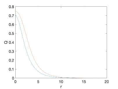
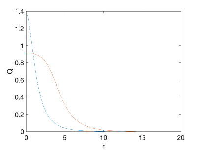
Figure 1. Ground state solutions $Q_{\omega=0.1}$ to the cubic NLS in blue and the cubic-quintic NLS in red: on the left for $d=2$ and on the right for $d=3$.

It can be seen that the situation is qualitatively different depending on the spatial dimension. Whereas in 2D, the cubic-quintic ground state has a slightly greater maximum and is slightly faster decaying than $Q_{\rm cubic}$, in 3D the cubic-quintic ground state has a much smaller maximum and a considerably larger support.

3.2. Numerical ground states in 2D

We first consider the case $d=2$ with $N=400$ collocation points: In Fig. 2 we show on the left a plot of the ground state function $Q_{\omega}(r)$ for various values of $\omega$. It is seen that the maximum of the ground states increases with $\omega$. The solutions also become more localized with increasing $\omega$. On the right of the same figure, we show the $L^{\infty}({\mathbb{R}}^{2})$-norm of the ground states as function of $\omega$. For convenience, we only consider values of $\omega\in[0.005,0.16]$.

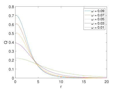
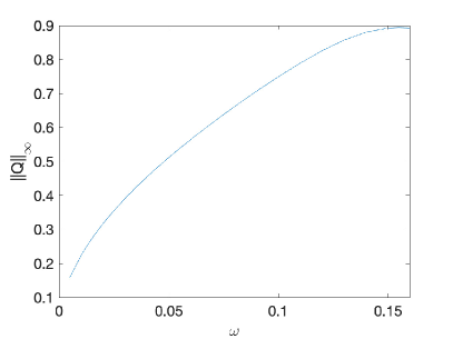
Figure 2. Left: Ground state solutions to (3.1) in dimension $d=2$ for several values of $\omega$. Right: The $L^{\infty}$-norm of these states as a function of $\omega$.

In Fig. 3 we depict the ground-state mass $M(Q_{\omega})$ and energy $E(Q_{\omega})$ as a function of $\omega$. These plots are based on a total library of roughly 100 numerical ground state solutions $Q$ on the shown range of $\omega$. The corresponding mass- and energy-integrals are thereby computed with the Clenshaw-Curtis algorithm in $s=r^{2}$, a spectral integration method based on the same Chebyshev collocation points as before, see [30]. Both $M(Q_{\omega})$ and $E(Q_{\omega})$ appear to be monotonic in $\omega$. In particular, the monotonicity of $M(Q)$ indicates orbital stability in the sense of Definition 1.2, in view of the Grillakis-Shatah-Strauss theory.

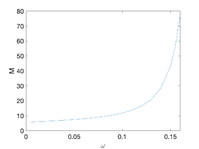
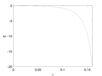
Figure 3. $M(Q_{\omega})$ and $E(Q_{\omega})$ as a functions of $\omega$ in dimension $d=2$.

3.3. Numerical ground states in 3D

In the case $d=3$, we use the same numerical parameters as before: In Fig. 4, we show on the left the ground states for several values of $\omega$. It can again be seen that the maximum of $Q_{\omega}$ increases with $\omega$, at least up to some value $\omega_{\ast}\approx 0.1$. For larger values of $\omega$, however, the $L^{\infty}({\mathbb{R}}^{3})$-norm of $Q_{\omega}$ is seen to be decreasing again.

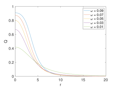
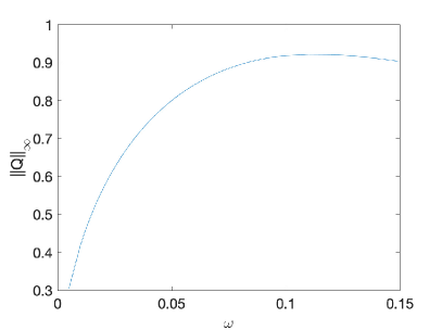
Figure 4. Left: Ground state solutions to (3.1) in dimension $d=3$ for several values of $\omega$. Right: The $L^{\infty}$-norm of these states as a function of $\omega$.

Analogously to the 2D case, the solutions become more localized with increasing $\omega$. Note, however, that despite its exponential decay, the 3D soliton is less localized than in the case of the purely focusing, cubic NLS, see Fig. 1 on the right. The 3D ground states in Fig. 4 on the left are also found to be less peaked than the corresponding solutions in dimension 2, see Fig. 2.

In contrast to the 2D case, the ground state mass $M(Q_{\omega})$ is no longer monotonically increasing as a function of $\omega$. Looking at Fig. 5, we see that, instead, $M(Q_{\omega})$ has a minimum at $\omega_{\rm crit}\approx 0.026$. We consequently expect orbital instability of ground states $Q_{\omega}$ for $\omega<\omega_{\rm crit}$, a phenomenon we shall study in more detail in Section 5.

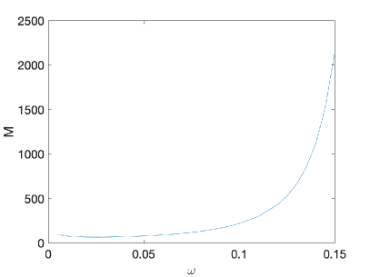
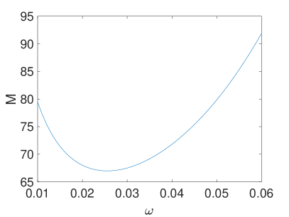
Figure 5. Left: $M(Q_{\omega})$ as a functions of $\omega$, for cubic-quintic ground states $Q_{\omega}$ in dimension $d=3$. Right: a close-up of the same curve near $\omega_{\rm crit}$.

In Fig. 6, the corresponding ground state energy $E(Q_{\omega})$ is seen to have a maximum at the same $\omega_{\rm crit}\approx 0.026$.

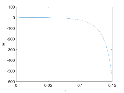
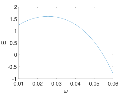
Figure 6. Left: $E(Q_{\omega})$ as a functions of $\omega$, for cubic-quintic ground states $Q_{\omega}$ in dimension $d=3$. Right: a close-up of the same curve near $\omega_{\rm crit}$.

The appearance of an unstable branch is clearly visible when the energy $E(Q_{\omega})$ is plotted as a function of the mass $M(Q_{\omega})$, see Fig. 7.

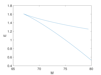
Figure 7. $E(Q_{\omega})$ as a function of $M(Q_{\omega})$ for cubic-quintic ground states in dimension $d=3$.

Our figure is in good agreement with [17, Figure 2] (where the constants are different because the factors are different from (1.1)). Clearly, ground states $\phi_{\omega}$ corresponding to the upper branch cannot correspond to constrained energy minimizers with mass $\rho=M(Q_{\omega})$.

4. Orbital stability of action ground states in 2D

4.1. Numerical method for the time-evolution

In this section we will numerically study the time-evolution of (1.1) resulting from initial data $u_{0}$ given by perturbations of action ground states. We will only consider perturbations which conserve the radial symmetry. To consider more general perturbations, a full 3D code would be necessary which is beyond the scope of the present paper. This allows us to use the change of variables (3.2) and effectively solve (1.1) in the (non-singular) form

(4.1) $$i\partial_{t}u+2s\frac{\partial^{2}u}{\partial s^{2}}+d\frac{\partial u}{\partial s}+|u|^{2}u-|u|^{4}u=0,\quad d=2,3.$$

We thereby use the same discretization for $s\in[0,\infty)$ in terms of Chebyshev collocation points as detailed in the previous section.

After the spatial discretization in $s$, equation (4.1) is then approximated via a system of ordinary differential equations. These equations are then integrated in time using a time-splitting method in which the linear step is solved numerically via an implicit fourth-order Runge-Kutta method, see [20] for more details. The accuracy of this time-integration algorithm is henceforth controlled via the analytically conserved quantity $E(u)$, which in our case nevertheless depends on time due to unavoidable numerical errors. As discussed in [18], the numerical conservation of the relative mass tends to overestimate the numerical error by one to two orders of magnitude. We shall always aim at a numerical error below $\mathcal{O}(10^{-3})$, i.e. below plotting accuracy. This means that we ensure a relative energy-conservation

$$\Delta_{E}=\left|\frac{E(t)}{E(0)}-1\right|$$

of order $\Delta_{E}=\mathcal{O}(10^{-5})$, or better.

We shall use a single computational domain $\Omega=[0,s_{0}]$ for which we impose a homogeneous Dirichlet condition $u(t,s_{0})=0$, for all $t\geqslant 0$. We mostly choose $s_{0}=10^{3}$, but in some unstable situations we shall also take $s_{0}=10^{4}$. As a basic test case, we first propagate the three-dimensional ground state $Q_{\omega}$, numerically found at $\omega=0.1$. We thereby use $N_{t}=10^{4}$ time-steps until a final time $t_{\rm f}=10$. We find that the hereby obtained numerical solution $u$, at $t=t_{\rm f}$, satisfies

$$\max_{\Omega}|u(t_{\rm f},\cdot)-e^{it_{\rm f}\omega}Q_{\omega}|=\mathcal{O}(10^{-9}),$$

i.e. the same order of accuracy as reached in [20].

Remark 4.1.

In general, it is not unproblematic to work with a homogeneous Dirichlet boundary condition on a finite numerical domain, since this could lead to unwanted reflections of the emitted radiation at the boundary, see, e.g., the discussion in [3]. In our case, however, only small, rapidly decreasing perturbations of ground states are considered. It is thus possible to work on sufficiently large computational domains $\Omega$, on which the radiation can separate from the bulk before spurious reflections from the boundary lead to noticeable effects.

4.2. Time-evolution of perturbed 2D ground states

In this subsection, we shall study the time-evolution of perturbed ground states to (1.1) in dimension $d=2$. To this end, we first consider the case where

(4.2) $$u_{0}(x)=\lambda Q_{\omega}(x),\quad\lambda>0.$$

Here $\lambda>0$ is a perturbation parameter and $Q_{\omega}$ is a numerically obtained action ground state, at a certain admissible frequency $\omega\in(0,\frac{3}{16})$.

We first study the case where $\omega=0.1$ and $\lambda=0.99$, and use $N_{t}=10^{4}$ time steps to reach the indicated final time $t_{\rm f}=20$. As expected, the solution $u$ to (1.1), effectively given by (4.1), is found to be close to the exact time-periodic state

$$\phi_{\omega}(t,x)=e^{i\omega t}Q_{\omega}(x).$$

To this end, we show on the left of Fig. 8 the $L^{\infty}({\mathbb{R}}^{2})$-norm of the solution as a function of time. It can be seen that it approaches a final state as $t\to 20$. The latter is found to be very close (in absolute value) to the unperturbed ground state $Q_{\rm\omega=0.1}$. Note that the $L^{\infty}$-difference is of the order of $10^{-4}$ and thus, much smaller than the initial perturbation.

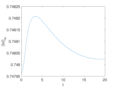
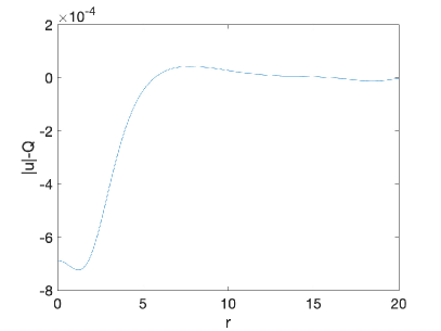
Figure 8. The 2D solution $u$ to (1.1) for initial data (4.2) with $\omega=0.1$ and $\lambda=0.99$. On the left the $L^{\infty}$-norm as a function of time. On the right the difference between $|u|$ and $Q_{\rm\omega=0.1}$ at the final time $t_{\rm f}=20$.

As a second case, we consider the same 2D initial data (4.2), but with $\lambda=1.001$. In Fig. 9 we again show the $L^{\infty}$-norm of the solution as a function of time. Similarly as before, a final state is reached and its maximum is again found to be very close to the unperturbed ground state $Q_{\omega=0.1}$. In both cases, we find that the difference is largest for $r$ close to the origin.

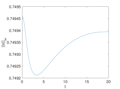
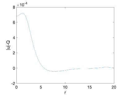
Figure 9. The 2D solution $u$ to (1.1) for initial data (4.2) with $\omega=0.1$ and $\lambda=1.001$. On the left the $L^{\infty}$-norm as a function of time. On the right the difference between $|u|$ and $Q_{\rm\omega=0.1}$ at the final time $t_{\rm f}=20$.

In order to illustrate that the qualitative picture found before is not due to our specific choice of perturbations, we shall also consider ground states perturbed by a small Gaussian-like perturbation, i.e.

(4.3) $$u_{0}(x)=Q_{\omega=0.1}(x)\pm\lambda e^{-|x|^{2}},\quad\lambda=0.001.$$

Note that we only consider smooth perturbations in this paper in order to allow for spectral accuracy in the radial coordinate, i.e., an exponential decrease of the numerical error with the number of collocation points. In Fig. 10 we show the behavior in time of the respective $L^{\infty}$-norms for the two choices $\pm\lambda$. In both situations the difference between $|u|$ at $t_{\rm f}=20$ and $Q_{\rm\omega=0.1}$ is found to be of the order $\mathcal{O}(10^{-4})$. Moreover, the error (not depicted here for the sake of readability) is again found to be largest close to the origin.

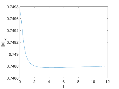
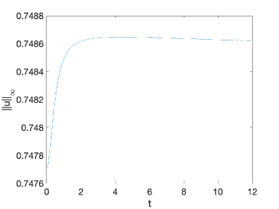
Figure 10. $L^{\infty}$-norm as a function of time for the 2D solution $u$ to (1.1) with initial data (4.3) and $\omega=0.1$. On the left the case with “$+$” sign. On the right the case with “$-$” sign.

If similar perturbations are applied to other ground states $Q_{\omega}$, the resulting solution $u$ behaves qualitatively similarly. Our numerical tests therefore support Conjecture 2.4. However, we also find that the smaller the choice of $\omega\in(0,\tfrac{3}{16})$, the longer it takes for the solution $u$ to reach its final state. In fact, for small enough $\omega$, damping effects within the time-oscillations of $|u|$ become almost invisible, even if one computes up to much larger times $t_{\rm f}=400$, see Fig. 11.

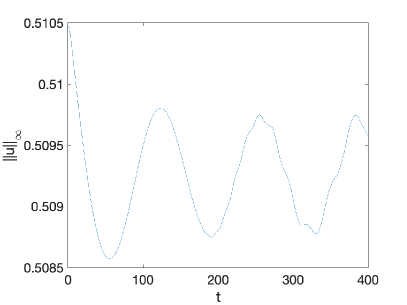
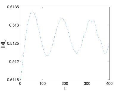
Figure 11. $L^{\infty}$-norm as a function of time for the 2D solution $u$ to (1.1) with initial data (4.3) and $\omega=0.05$. On the left the case with the “$+$” sign. On the right the case with the “$-$” sign.

5. (In-)stability of action ground states in 3D

5.1. Stable branch

In this section, we shall study the question of (in-)stability of cubic-quintic ground states in dimension $d=3$. In view of Fig. 5, we expect ground states $Q_{\omega}$ with $\omega>\omega_{\rm crit}\approx 0.026$ to be orbitally stable. That this is indeed the case, is strongly suggested by our numerical results below.

To this end, we first consider multiplicative perturbations of $Q_{\rm\omega}$ on the stable branch: In Figures 12 and 13 we study the time-evolution of (1.1) with initial data of the form (4.2). On the left of Fig. 12 we show the $L^{\infty}$-norm of the solution $u$ obtained in the case $\omega=0.1$ and $\lambda=0.99$. On the right of the same figure, we show the difference between the unperturbed ground state $Q_{\rm\omega=0.1}$ and $|u|$ at the final time $t_{\rm f}=15$. It can be seen that the $L^{\infty}$ norm settles on a nearly constant value as $t\to 15$.

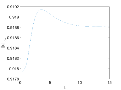
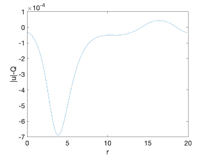
Figure 12. The 3D solution $u$ to (1.1) for initial data (4.2) with $\omega=0.1$ and $\lambda=0.99$. On the left the $L^{\infty}$-norm as a function of time. On the right the difference between $|u|$ and $Q_{\rm\omega=0.1}$ at the final time $t_{\rm f}=15$.

In Fig. 13 we study the analogous situation with $\lambda=1.001$: Again, the (absolute value of the) solution $u$ seems to settle around $t_{\rm f}=15$ on the stable unperturbed ground state $Q_{\rm 0.1}$. In both cases, the error between $|u|$ and $Q_{\rm\omega=0.1}$ is again found to be of the order $\mathcal{O}(10^{-4})$.

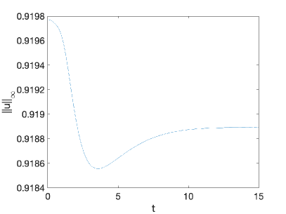
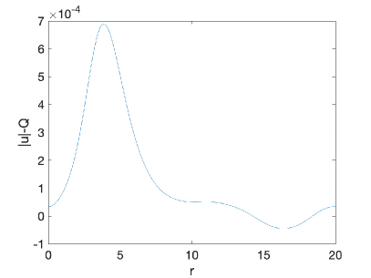
Figure 13. The 3D solution $u$ to (1.1) for initial data (4.2) with $\omega=0.1$ and $\lambda=1.001$. On the left the $L^{\infty}$-norm as a function of time. On the right the difference between $|u|$ and $Q_{\rm\omega=0.1}$ at the final time $t_{\rm f}=15$.

5.2. Unstable branch

The situation dramatically changes if we consider perturbations of ground state solutions on the unstable branch, i.e. perturbations of $Q_{\omega}$ with $\omega<\omega_{\rm crit}\approx 0.026$:

In Fig. 14 we show the solution $u$ to (1.1) obtained from initial data (4.2) with $\omega=0.01$ and $\lambda=0.999$. Note that this implies $M(u_{0})<M(Q_{\omega})$. The solution is seen to be purely dispersive which is also confirmed by the $L^{\infty}$-norm of the solution as a function of time (depicted on the right of the same figure). In fact, we did not discover any stable structure within the time-evolution even if we let the numerical code run for longer times.

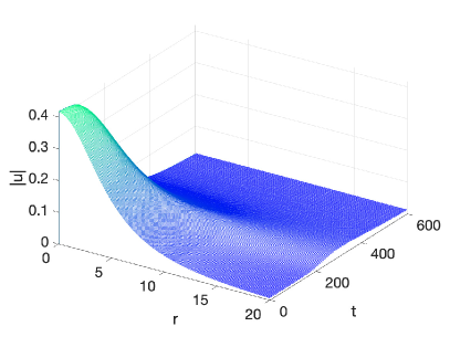
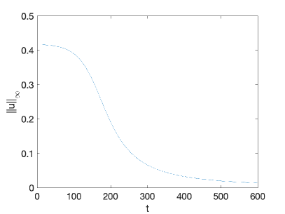
Figure 14. Left: The absolute value of the solution $u$ to (1.1) in dimension $d=3$ obtained from initial data (4.2) with $\omega=0.01$ and $\lambda=0.999$. Right: The $L^{\infty}$-norm of $u$ as a function of time.

If we consider the same ground state as before, but instead choose $\lambda=1.001$, we find a different kind of instability. Now the solution $u$ shows oscillations of high amplitude, see Figure 15.

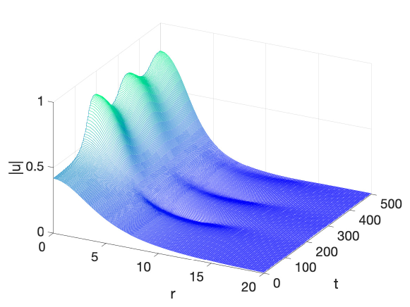
Figure 15. Solution to (1.1) in dimension $d=3$ for initial data (4.2) with $\omega=0.01$ and $\lambda=1.001$.

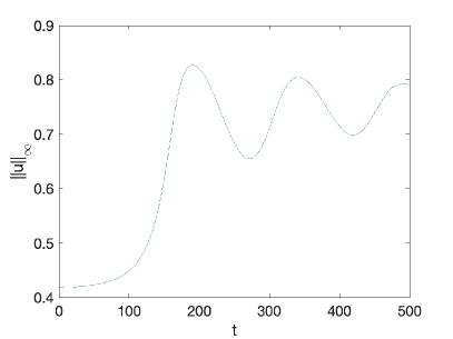
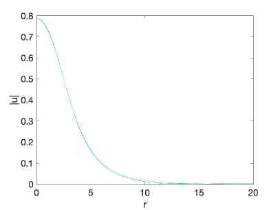
Figure 16. Solution to (1.1) in dimension $d=3$ for initial data (4.2) with $\omega=0.01$ and $\lambda=1.001$: On the left the $L^{\infty}$-norm of $u$ as a function of time. On the right $|u|$ at the final time (in blue) together with the ground state $Q_{\omega=0.047}$ (in green).

These oscillations are even more visible in the $L^{\infty}$-norm of the solution, as depicted on the left of Fig. 16. One can see that early on the norm is growing strongly but then it appears to show damped oscillations around some final state. We conjecture that the latter corresponds to another ground state on the stable branch. To this end, we compare the maximum of $|u|$, obtained at the final time $t_{\rm f}=500$, with the $L^{\infty}$-norms in our library of previously computed action ground states $Q_{\rm\omega}$, cf. Fig. 4. Indeed we find good agreement of $|u|$, when compared to $Q_{\omega}$ with $\omega=0.047>\omega_{\rm crit}$, see the right of Fig. 16. Thus perturbations of unstable ground states where $M(u_{0})>M(Q_{\omega})$, seem to result in solutions which eventually settle on another, stable ground state as $t\to+\infty$. Note, however, that $M(Q_{\omega=0.01})\approx 79.44$ while $M(Q_{\omega=0.047})\approx 77.05$. If the final state had the same mass as the unperturbed initial state, this would correspond to an $\omega\approx 0.0495$. This shows that a certain amount of mass is lost through radiation.

5.3. Other kinds of perturbations

The results described above are not due to our specific choice of perturbations. To show this, we consider initial data

(5.1) $$u_{0,\pm}(x)=Q_{\omega}(x)\pm\lambda e^{-\left(|x|-|x_{0}|\right)^{2}},\quad\lambda=0.001.$$

For both $|x_{0}|=0$ and $|x_{0}|\not=0$, the solution in the case with the “$+$” sign looks very similar to the one depicted in Fig. 16. This fact becomes particularly clear when one compares the time-evolution of the $L^{\infty}$-norm of $u$ depicted in Fig. 17, with the one from Fig. 16.

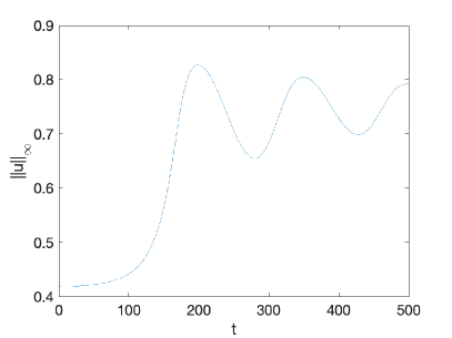
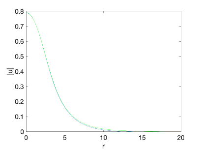
Figure 17. Solution to (1.1) in dimension $d=3$ for initial data of the form (5.1) with $|x_{0}|=1$, and $\omega=0.01$: On the left the $L^{\infty}$-norm of $u$ as a function of time. On the right $|u|$ at the final time (in blue) together with the ground state $Q_{\omega=0.048}$ (in green).

By comparing the maximum of $|u|$ found at the final time $t_{\rm f}=600$ with the $L^{\infty}$-norm of a stable ground state, we find good agreement with $Q_{\omega=0.048}$. The latter has mass $M(Q_{\omega=0.048})\approx 77.95$. Unfortunately, we are unable to clearly decide whether the final state is closer to $Q_{\omega=0.048}$ than to $Q_{\omega=0.047}$.

In the case of initial data (5.1) with the “$-$” sign, we again find that the solution is completely dispersed, see Fig. 18. This is consistent with our earlier findings above which indicate that perturbation with $M(u_{0})<M(Q_{\omega})$ lead to purely dispersive solutions.

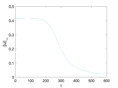
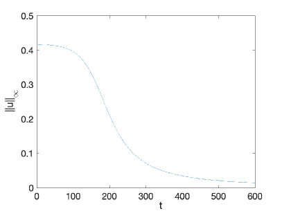
Figure 18. The $L^{\infty}$-norm of the solution $u$ in dimension $d=3$ obtained from initial data (5.1) with the “$-$” sign. On the left the case with $x_{0}=0$ and on the right the one with $x_{0}=1$.

We finally note that the situation is qualitatively similar for other values of $\omega$ on the unstable branch. In our last example, we choose $\omega=0.007<\omega_{\rm crit}$ within the initial $u_{0}$ given by (5.1). We again find that perturbations with an initial mass smaller than $M(Q_{\omega=0.007})$ are purely dispersive. Perturbations with mass larger than $M(Q_{\omega=0.007})$ lead to damped oscillations around some final state, see Fig. 19.

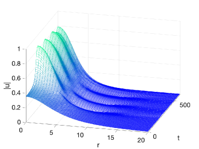
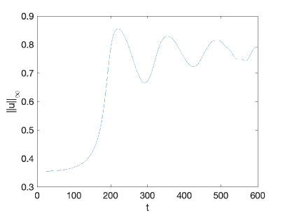
Figure 19. Left: Solution to (1.1) in dimension $d=3$ for initial data (5.1) with $x_{0}=0$ and $\omega=0.007$. Right: The $L^{\infty}$-norm of $u$ as a function of time.

The asymptotic final state appears to be close to $Q_{\omega=0.044}$ on the stable branch. The mass of the unperturbed initial data $M(Q_{\omega=0.007})\approx 90.57$ is seen to be bigger than $M(Q_{\omega=0.044})\approx 75.37$, showing again that a non-negligible part of the initial mass has been radiated away.

The numerical results within this subsection can then be summarized as follows:

Conjecture 5.1.

For $\omega<\omega_{c}$, consider initial data of the form

$$u_{0}(x)=Q_{\omega}(x)+\epsilon(|x|),\ \text{ with $\|\epsilon\|_{H^{1}}\ll 1$.}$$

• If $M(u_{0})<M(Q_{\omega})$, then the solution $u$ to (1.1) is purely dispersive;

• If $M(u_{0})>M(Q_{\omega})$, then the solution to (1.1) converges, as $t\to+\infty$, to a solitary wave $\phi_{\underline{\omega}}(t,x)=e^{i\underline{\omega}t}Q_{\underline{\omega}}(x)$ plus radiation, where $Q_{\underline{\omega}}$ is a stable ground state with mass smaller that the unstable one, $M(Q_{\underline{\omega}})<M(Q_{\omega})$.

Remark 5.2.

The same instability scenario was found (numerically) for perturbed solitary wave solutions to the generalized BBM equation in [4], and for a version of NLS with derivative nonlinearity in [2]. In particular, analogously to our situation, a perturbation which lowered the mass of the initial data below the one of the (unstable) solitary wave always resulted in purely dispersive solutions. In all of these cases, it remains an interesting open question to find a possible selection criterion for the specific value $\underline{\omega}$ which describes the (stable) asymptotic state $\phi_{\underline{\omega}}$.

References

- [1] F. K. Abdullaev, A. Gammal, L. Tomio, and T. Frederico, Stability of trapped Bose-Einstein condensates, Phys. Rev. A, 63 (2001), p. 043604.
- [2] J. Arbunich, C. Klein, and C. Sparber, On a class of derivative nonlinear Schrödinger-type equations in two spatial dimensions, ESAIM Math. Model. Numer. Anal., 53 (2019), pp. 1477–1505.
- [3] M. Birem and C. Klein, Multidomain spectral method for Schrödinger equations, Adv. Comput. Math., 42 (2016), pp. 395–423.
- [4] J. L. Bona, W. R. McKinney, and J. M. Restrepo, Stable and unstable solitary-wave solutions of the generalized regularized long-wave equation, J. Nonlinear Sci., 10 (2000), pp. 603–638.
- [5] V. S. Buslaev and V. E. Grikurov, Simulation of instability of bright solitons for NLS with saturating nonlinearity, Math. Comput. Simulation, 56 (2001), pp. 539–546.
- [6] J. Byeon, L. Jeanjean, and M. Mariş, Symmetry and monotonicity of least energy solutions, Calc. Var. Partial Differential Equations, 36 (2009), pp. 481–492.
- [7] R. Carles and C. Sparber, Orbital stability vs. scattering in the cubic-quintic Schrödinger equation, Rev. Math. Phys., 33 (2021), no. 3, 2150004.
- [8] T. Cazenave, Semilinear Schrödinger equations, vol. 10 of Courant Lecture Notes in Mathematics, New York University Courant Institute of Mathematical Sciences, New York, 2003.
- [9] T. Cazenave and P.-L. Lions, Orbital stability of standing waves for some nonlinear Schrödinger equations, Comm. Math. Phys., 85 (1982), pp. 549–561.
- [10] S. Cingolani, L. Jeanjean, and S. Secchi, Multi-peak solutions for magnetic NLS equations without non-degeneracy conditions, ESAIM Control Optim. Calc. Var., 15 (2009), pp. 653–675.
- [11] S. De Bièvre, F. Genoud, and S. Rota Nodari, Orbital stability: analysis meets geometry, in Nonlinear optical and atomic systems, vol. 2146 of Lecture Notes in Math., Springer, Cham, 2015, pp. 147–273.
- [12] A. Gammal, T. Frederico, L. Tomio, and P. Chomaz, Atomic Bose-Einstein condensation with three-body intercations and collective excitations, J. Phys. B, 33 (2000), pp. 4053–4067.
- [13] V. E. Grikurov, Soliton’s rebuilding in one-dimensional Schrödinger model with polynomial nonlinearity. IMA Preprint Series# 1320., 1995.
- [14] M. Grillakis, J. Shatah, and W. Strauss, Stability theory of solitary waves in the presence of symmetry. I, J. Funct. Anal., 74 (1987), pp. 160–197.
- [15] I. D. Iliev and K. P. Kirchev, Stability and instability of solitary waves for one-dimensional singular Schrödinger equations, Differential Integral Equ., 6 (1993), pp. 685–703.
- [16] L. Jeanjean and S.-S. Lu, On global minimizers for a mass constrained problem, preprint, 2021, archived as https://arxiv.org/abs/2108.04142.
- [17] R. Killip, T. Oh, O. Pocovnicu, and M. Vişan, Solitons and scattering for the cubic-quintic nonlinear Schrödinger equation on , Arch. Ration. Mech. Anal., 225 (2017), pp. 469–548.
- [18] C. Klein, Fourth order time-stepping for low dispersion Korteweg-de Vries and nonlinear Schrödinger equations, Electron. Trans. Numer. Anal., 29 (2007/08), pp. 116–135.
- [19] C. Klein, C. Sparber, and P. Markowich, Numerical study of fractional nonlinear Schrödinger equations, Proc. R. Soc. Lond. Ser. A Math. Phys. Eng. Sci., 470 (2014), pp. 20140364, 26.
- [20] C. Klein and N. Stoilov, Numerical study of the transverse stability of the Peregrine solution, Stud. Appl. Math., 145 (2020), pp. 36–51.
- [21] B. J. LeMesurier, G. Papanicolaou, C. Sulem, and P.-L. Sulem, Focusing and multi-focusing solutions of the nonlinear Schrödinger equation, Phys. D, 31 (1988), pp. 78–102.
- [22] M. Lewin and S. Rota Nodari, Uniqueness and non-degeneracy for a nuclear nonlinear Schrödinger equation, NoDEA Nonlinear Differential Equations Appl., 22 (2015), pp. 673–698.
- [23] , The double-power nonlinear Schrödinger equations and its generalizations: uniqueness, non-degeneracy and applications, Calc. Var. Partial Differ. Equ., 59 (2020), paper no. 197, 48 p.
- [24] B. Malomed, Vortex solitons: Old results and new perspectives, Physica D, 399 (2019), pp. 108–137.
- [25] H. Michinel, J. Campo-Táboas, R. García-Fernández, J. R. Salgueiro, and M. L. Quiroga-Teixeiro, Liquid light condensates, Phys. Rev. E, 65 (2002), p. 066604.
- [26] M. Ohta, Stability and instability of standing waves for one-dimensional nonlinear Schrödinger equations with double power nonlinearity, Kodai Math. J., 18 (1995), pp. 68–74.
- [27] K. I. Pushkarov, D. I. Pushkarov, and I. V. Tomov, Self-action of light beams in nonlinear media: soliton solutions, Optical Quantum Electronics, 11 (1979), pp. 471–478.
- [28] C. Sulem and P.-L. Sulem, The nonlinear Schrödinger equation, Self-focusing and wave collapse, Springer-Verlag, New York, 1999.
- [29] T. Tao, M. Visan, and X. Zhang, The nonlinear Schrödinger equation with combined power-type nonlinearities, Comm. in Partial Diff. Eq., 32 (2007), pp. 1281–1343.
- [30] L. N. Trefethen, Spectral methods in MATLAB, vol. 10 of Software, Environments, and Tools, Society for Industrial and Applied Mathematics (SIAM), Philadelphia, PA, 2000.
- [31] J. A. C. Weideman and S. C. Reddy, A MATLAB differentiation matrix suite, ACM Trans. Math. Software, 26 (2000), pp. 465–519.
- [32] M. I. Weinstein, Nonlinear Schrödinger equations and sharp interpolation estimates, Comm. Math. Phys., 87 (1982/83), pp. 567–576.
- [33] M. I. Weinstein, Modulational stability of ground states of nonlinear Schrödinger equations, SIAM J. Math. Anal., 16 (1985), pp. 472–491.
- [34] X. Zhang, On the Cauchy problem of 3-D energy-critical Schrödinger equations with subcritical perturbations, J. Differential Equ., 230 (2006), pp. 422–445.