Observations of Ly$\alpha$ Emitters at High Redshift

Abstract

In this series of lectures, I review our observational understanding of high-$z$ Ly$\alpha$ emitters (LAEs) and relevant scientific topics. Since the discovery of LAEs in the late 1990s, significant progresses in LAE studies have been made over the past two decades by deep multi-wavelength observations. More than ten (one) thousand(s) of LAEs have been identified photometrically (spectroscopically) in optical and near-infrared data, and the redshifts of these LAEs range from $z\sim 0$ to $z\sim 10$. These large samples of LAEs are useful to address two major astrophysical issues, galaxy formation and cosmic reionization. Statistical studies have revealed the general picture of LAEs’ physical properties: young stellar populations, remarkable luminosity function evolutions, compact morphologies, highly ionized inter-stellar media (ISM) with low metal/dust contents, low masses of dark-matter halos. Typical LAEs represent low-mass high-$z$ galaxies, high-$z$ analogs of dwarf galaxies, some of which are thought to be candidates of population III galaxies. These observational studies have also pinpointed rare bright Ly$\alpha$ sources extended over $\sim 10-100$ kpc, dubbed Ly$\alpha$ blobs, whose physical origins are under debate. LAEs are used as probes of cosmic reionization history through the Ly$\alpha$ damping wing absorption given by the neutral hydrogen of the inter-galactic medium (IGM), which complement the cosmic microwave background radiation and 21cm observations targeting the epoch of reionization. The low-mass and highly-ionized population of LAEs can be major sources of cosmic reionization, and physical parameters including the ionizing photon escape fraction have been extensively investigated. The budget of ionizing photons for cosmic reionization has been constrained, although there remain large observational uncertainties in the parameters. Beyond these two established topics of LAEs, galaxy formation and cosmic reionization, several new usages of LAEs for science frontiers have been suggested such as the distribution of Hi gas in the circum-galactic medium and filaments of large-scale structures. On-going 10 m-class optical telescope programs and future telescope projects, such as JWST, ELTs, and SKA, will address the remaining open questions related to LAEs, and push the horizons of the science frontiers.

1 Introduction

About two decades have passed since the observational discovery of Ly$\alpha$ emitters (LAEs) at high redshift. Before then, early theoretical studies focused on discussing young primordial galaxies with strong Ly$\alpha$ emission. However, after the discovery, observations have revealed a number of exciting characteristics of LAEs, some of which are beyond the theoretical predictions. In this section, I show the growing importance of LAE studies, overviewing the LAE observation history through the early theoretical predictions, the discovery, and new problems in this observational field. Throughout this lecture, magnitudes are in the AB system, if not otherwise specified. All physical values are calculated with the concordance cosmology of $H_{0}=100h$ km s^-1 Mpc^-1 with $h\simeq 0.7$, ${\rm\Omega_{m}}\simeq 0.3$, ${\rm\Omega_{\Lambda}}\simeq 0.7$, ${\rm\Omega_{b}}h^{2}\simeq 0.02$, $\sigma_{8}\simeq 0.8$, and $n_{s}\simeq 1.0$ that are consistent with the latest Planck2016 cosmology (Planck Collaboration et al., 2016).

1.1 Predawn of the LAE Observation History

Theoretical Predictions

Partridge & Peebles (1967a) is the first well-known study that discusses galaxies emitting strong Ly$\alpha$ at high redshift, which are called LAEs today. Partridge & Peebles (1967a) predict that an early galaxy emits a strong hydrogen Ly$\alpha$ line through the recombination process in the inter-stellar medium (ISM) that is heated by young massive stars (Figure 1). As much as 6-7% of the total galaxy luminosity can be converted to Ly$\alpha$ luminosity in a Milky Way mass halo. Assuming a high star-formation rate that converts $2$% of hydrogen to metal within $3\times 10^{7}$ yr in a Milky Way mass halo, Partridge & Peebles (1967a) suggest that such galaxies would have an extremely bright Ly$\alpha$ luminosity of $\sim 2\times 10^{45}$ erg s^-1 at $z\sim 10-30$. Interestingly, Partridge & Peebles (1967a) discuss the observability of those young Ly$\alpha$ emitting galaxies, taking the effects of cosmic reionization into account (see also a companion paper, Partridge & Peebles 1967b). Here, Partridge & Peebles (1967a) introduce a possible strong free-electron scattering in the ionized IGM that smears the radiation from the young galaxies, which is an argument that differs from today’s major discussion on the absorption of Ly$\alpha$ emission by the neutral IGM. Although their discussion of young galaxies’ Ly$\alpha$ luminosities and reionization effects on the Ly$\alpha$ observability is very different from the present-day one, it is interesting to notice that the two major cosmological topics discussed today in relation with LAEs, namely galaxy formation and cosmic reionization, had already been studied theoretically in the 1960s.

Figure 1: Expected spectrum of a young galaxy (Partridge & Peebles, 1967a). Here, $\Delta\nu=0.002\nu$ is assumed for the line width. This figure is reproduced by permission of the AAS.

Early Searches for LAEs

Since the theoretical predictions of Partridge & Peebles (1967a) were published, a number of observational projects searched for young LAEs at $z\sim 2-6$ (e.g. Koo & Kron 1980; Pritchet & Hartwick 1987, 1990; Djorgovski & Thompson 1992; Thompson et al. 1995). These observational searches were conducted in the 1980s and 1990s with 4m-class optical telescopes including the Palomar 200-inch Hale telescope that was the largest aperture telescope used for researches before the 10m Keck I telescope became available. Although many candidates were pinpointed by narrowband imaging and slitless spectroscopy in these searches, no real young LAEs at $z\mathrel{\hbox{\hbox to0.0pt{\hbox{\lower 4.0pt\hbox{$\sim$}}\hss}\hbox{$>$}}}2$ were confirmed by spectroscopy. However, these null-detection results placed meaningful upper limits on the luminosity function of LAEs (Figure 2).

Figure 2: One sigma upper limits of Ly$\alpha$ luminosity functions at $z=2-9$ (black solid and dashed lines). The black arrow indicates the offset value between one and three sigma levels that can allow us to convert the one to three sigma upper limits. The red curve is the approximate Ly$\alpha$ luminosity function of LAEs at $z=2-5$ obtained thus far (e.g. Gronwall et al. 2007; Ouchi et al. 2008; Cassata et al. 2011). The black curve is the model Ly$\alpha$ luminosity function. The blue (green) line represents a typical observational limit of a narrow-field (wide-field) imager mounted on an 8m (4m) class telescope. All numbers quoted in this figure hold for a cosmological model with $H_{0}=75$ km s^-1 Mpc^-1, ${\rm\Omega_{m}}=0.2$, and ${\rm\Omega_{\Lambda}}=0.0$. This figure is adopted from Figure 13 of Thompson et al. (1995), and reproduced by permission of the AAS.

Discovery

Since 1996, LAE observations have entered a new era. Hu & McMahon (1996) have identified two LAEs at $z=4.55$ around the QSO BR2237-0607 using the Keck LRIS spectrograph (Figure 3), after having detected them using deep UH88 imaging through a narrow band filter with the central wavelength tuned to the wavelength of Ly$\alpha$ emission at $z=4.55$. At the same time, Pascarelle et al. (1996a) discovered 5 LAEs, including a weak AGN, around the radio galaxy 53W002 at $z=2.39$ using

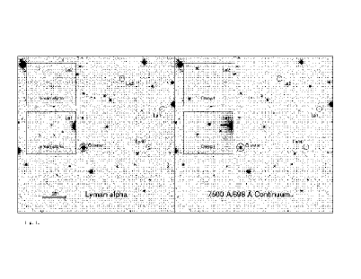
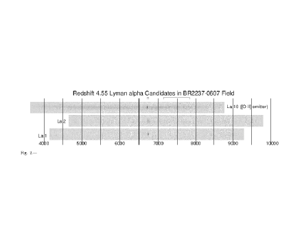
Figure 3: Top: Images of three LAE candidates in the QSO field of BR2237-0607 at $z=4.55$ marked with the small circles (Hu & McMahon, 1996). The QSO is indicated with the large circle. The left and right panels present narrowband and broadband images, respectively, that cover the redshifted Ly$\alpha$ emission and the rest-frame UV continua of the LAEs. Bottom: Two-dimensional spectra of the three LAE candidates (Hu & McMahon, 1996). Clear Ly$\alpha$ signals of the LAE candidates are found in the wavelength between 6500 and 7000Å. The two objects in the two lower panels are LAEs, while the object in the top panel is classified as a low-$z$ [Oii] emitter. This figure is reproduced by permission of the Nature Publishing Group.

the Hubble Space Telescope (HST) for broadband imaging, a ground based telescope for narrowband imaging, and the MMT for spectroscopy. Pascarelle et al. (1996b) claim that such LAEs form a galaxy group in the 53W002 region. These discovered LAEs have Ly$\alpha$ luminosities of a few times $10^{42}$ erg s^-1 that is about $1/100$ of the young galaxies predicted by Partridge & Peebles (1967a).

These early studies found LAEs in the vicinity of AGNs that are thought to be signposts of high-$z$ galaxy overdensities. LAEs in blank fields were first identified by Cowie & Hu (1998) and Hu et al. (1998) who carried out Keck LRIS narrowband imaging and spectroscopy in the SSA22 and Hubble Deep Field (HDF). Such deep field observations started to identify LAEs at $z\mathrel{\hbox{\hbox to0.0pt{\hbox{\lower 4.0pt\hbox{$\sim$}}\hss}\hbox{$>$}}}2$ in blank fields routinely with the high sensitivities of 8m class telescopes and the large-area survey capabilities of 4-8m class telescopes around the year 2000. These deep field observation programs include the Hawaii Survey (Cowie & Hu, 1998), the Large Area Lyman Alpha Survey (LALA; Rhoads et al. 2000), the Subaru Surveys (e.g. Ouchi et al. 2003), and the Multiwavelength Survey by Yale-Chile (MUSYC; Gawiser et al. 2007), and recently an LAE search with a new technology has been demonstrated by the HETDEX Pilot Survey (HPS: Adams et al. 2011) . Recent space based observations even find LAEs at $z\sim 0$ whose Ly$\alpha$ emission lines fall in the far UV wavelength range. There is an HST survey program, the so-called Lyman-Alpha Reference Sample (LARS; Östlin et al. 2014) that investigates the Ly$\alpha$ properties of star-forming galaxies originally selected as H$\alpha$ emitters at $z\sim 0$. Moreover, far and near UV grism data from the Galaxy Evolution Explorer (GALEX) are used to detect LAEs at $z\sim 0-1$ and to build Ly$\alpha$ flux limited samples for studies of Ly$\alpha$ luminosity functions (Section 3.2; Deharveng et al. 2008; Cowie et al. 2010, 2011). For more details about $z\sim 0$ LAE observations, see M. Hayes’ lectures in this course.

There is a question why no single LAE at high-$z$ could be identified by the observations until 1996, about two decades after the predictions of Partridge & Peebles (1967a). As shown in Figure 2, the blank field surveys conducted until 1995 found no LAEs at $z>2$ down to number densities of $\sim 10^{-4}$ Mpc^-3 at $L({\rm Ly\alpha})=10^{43}$ erg s^-1 and $\sim 10^{-3}$ Mpc^-3 at $L({\rm Ly\alpha})=10^{42}$ erg s^-1. These number-density limits just touch the Ly$\alpha$ luminosity functions at $z\sim 3-5$ that have been determined to date (see Section 3.2). In other words, one could have found LAEs in a blank field before 1996, if there was a one-more push of sensitivity or survey volume. However, such a one-more push was not made until 1996. In reality, there are two important approaches leading to these successful detections of LAEs. The first approach is to focus on AGN regions. The first LAE detections (Hu & McMahon, 1996; Pascarelle et al., 1996a) were accomplished in AGN regions, whose galaxy overdensities enhance the probability of bright LAEs existing in the survey area, resulting in successful selections and spectroscopic confirmations even with 2-4 m class telescopes. The second approach is to exploit the great sensitivity of 8m-class telescopes newly available since the 1990s. In fact, the Keck deep narrowband observations by Cowie & Hu (1998) successfully identified LAEs in blank fields. Interestingly, these two approaches provided successful detections almost at the same time in the late 1990s.

Around the year 2000, wide-field optical imagers started operation in 4m-class telescopes (e.g. KPNO/MOSAIC), allowing the observers to detect LAEs in blank fields even with the moderately low sensitivity of 4m-class telescopes (Rhoads et al. 2000; Gawiser et al. 2007; Figure 2). Moreover, after the first light of the wide-field optical imager Suprime-Cam on the 8m-Subaru telescope in 1999, large LAE surveys cover wider sensitivity and volume ranges, in contrast with the previous narrow-field 8m-class observations (Figure 2). The deep spectroscopic capabilities of the Keck, VLT, and Subaru telescopes are also key for confirmation of faint LAE candidates that are found in blank fields.

Definition of LAEs

Here I introduce the definition of LAEs, although it should be noted that some detailed definitions depend on the study considered. Nowadays, the widely accepted definition of LAEs is: LAEs are galaxies with a Ly$\alpha$ rest-frame equivalent width ($EW_{0}$) greater than $\simeq 20$ Å. The criterion of Ly$\alpha$ $EW_{0}\mathrel{\hbox{\hbox to0.0pt{\hbox{\lower 4.0pt\hbox{$\sim$}}\hss}\hbox{$>$}}}20$ Å is historically determined by the realistic selection limit of narrowband imaging surveys for Ly$\alpha$ emitting galaxies at $z\sim 3$. By this definition, the main contribution to the LAE population consists of star-forming galaxies, some of which have AGN activity.

LAE Search Techniques

There are two popular techniques to search for LAEs. One is narrowband imaging. Figure 4 illustrates the idea. The redshifted Ly$\alpha$ emission of LAEs is identified by a flux excess in a narrowband image over other wavelength images (Figure 4). The central wavelength of the narrowband filter, $\lambda_{\rm c}$, determines the redshift of the target LAEs that is roughly given by $\lambda_{\rm c}/1216-1$. The $\lambda_{\rm c}$ value of a narrowband filter is chosen by a scientific requirement (i.e., redshift of target LAEs) and/or observational constraints (e.g. avoiding weak night-sky OH emission lines). In most cases, $\lambda_{\rm c}$ is placed in an OH emission window (bottom panel of Figure 4) to realize a high sensitivity.

The other technique is blind spectroscopy, including slitless spectroscopy. Figure 5 shows one example that uses a VLT/FORS grism targeting a blank sky field with no prior positional information of a LAE candidate (Kurk et al., 2004). The LAE candidate is found as a single-line emitter in the grism image. Although this technique provides positions and spectra of LAEs at the same time, the background sky level is high in the slitless data. Thus, HST grism observations are popular to perform slitless spectroscopic searches for LAEs, exploiting the low sky background in space (Pirzkal et al., 2004). The blind spectroscopy technique also includes slit spectroscopy such as long-slit spectroscopy conducted on positions of critical lines of lensing clusters searching for lensed LAEs (Santos et al., 2004). Moreover, the recent advancement of integral field spectrographs (IFSs) allows blind spectroscopic searches for LAEs in reasonably large areas, keeping the background sky sufficiently low (van Breukelen et al., 2005; Bacon et al., 2015).

Figure 4: Illustration of the narrowband selection for an LAE at $z=6.6$ (NB921-C-106098). The top panel presents images of this LAE observed with broadbands ($B$, $V$, $R$, $i^{\prime}$, and $z^{\prime}$) and a narrowband ($NB$) whose central wavelength is $\sim 9200$Å. The second top panel is a spectrum of this LAE in the wavelength range of $9050-9275$Å. The third top panel shows the model spectrum of a LAE redshifted to $z\sim 6.6$. The second bottom panel exhibits the transmission curves of the broadbands and the narrowband. The bottom panel presents the atmospheric OH lines. Some images of this figure are taken from Ouchi et al. (2010). This figure is reproduced by permission of the AAS.

Figure 5: An LAE candidate found in VLT/FORS grism data in a blank field (Kurk et al., 2004), labeled on the image. An [Oiii]5007 emitter is also found at the upper right of this image. This figure is reproduced by permission of A&A.

Although these two techniques are major ones for identifying LAEs, recent deep spectroscopy has found continuum-selected galaxies (e.g. dropouts or Lyman break galaxies; LBGs) with a spectroscopic measurement of Ly$\alpha$ $EW_{0}\mathrel{\hbox{\hbox to0.0pt{\hbox{\lower 4.0pt\hbox{$\sim$}}\hss}\hbox{$>$}}}20$Å that are also classified as LAEs (e.g. Erb et al. 2014). In this series of lectures, LAEs include continuum-selected galaxies with Ly$\alpha$ $EW_{0}\mathrel{\hbox{\hbox to0.0pt{\hbox{\lower 4.0pt\hbox{$\sim$}}\hss}\hbox{$>$}}}20$Å.

1.2 Progresses in LAE Observational Studies After the Discovery

Large survey programs have so far identified a total of more than $10^{4}$ LAEs up to $z\sim 8$ photometrically (e.g. Yamada et al. 2012a; Konno et al. 2016), out of which about $10^{3}$ have been spectroscopically confirmed (e.g. Hu et al. 2010; Kashikawa et al. 2011). Due to the high abundance (i.e. number density) of LAEs, $10^{-3}$ Mpc^-3 at $L_{\rm Ly\alpha}\sim 10^{42}-10^{43}$ erg s^-1, LAEs are thought to constitute one of the major populations of high-$z$ galaxies. Below, I highlight progresses in LAE observations that are detailed in Sections 3-LABEL:sec:cosmic_reionizationII.

Deep photometric studies reveal the average spectral energy distribution (SED) of LAEs with deep optical and NIR photometric data. From comparisons with stellar population synthesis models, stellar population, one of the basic properties of galaxies, is studied (e.g. Gawiser et al. 2007; Finkelstein et al. 2007; Ono et al. 2010a, b; Guaita et al. 2011; Hagen et al. 2014, 2016). Figure 6 compares LAEs’ average stellar masses ($M_{\rm s}$) and specific star-formation rates (sSFRs), defined as the star-formation rate (SFR) divided by stellar mass, with those of other galaxy populations: LBGs, distant-red galaxies (DRGs), and sub-millimeter galaxies (SMGs) at $z\sim 3$. The average $M_{\rm s}$ of LAEs is $10^{8}-10^{9}M_{\odot}$, which falls in the lowest mass range among the high-$z$ galaxy populations (Section 3.1). The low stellar masses of the LAEs suggest that LAEs are high-$z$ analogs of local star-forming dwarf galaxies. The sSFR values of LAEs are comparable to or slightly higher than those of the other high-$z$ galaxies, although the distribution of LAEs at the low-mass limit of Figure 6 is biased by the observational selection limits.

Figure 6: sSFR as a function of stellar mass for typical LAEs (blue symbols), LBGs/dropouts (black open squares), DRGs (black open circles), and SMGs (star marks) at $z=3$ (Ono et al., 2010a). The thick ovals indicate the approximated distributions of LAEs (blue), LBGs/dropouts (orange), DRGs (magenta), and SMGs (red). The red squares and circles with error bars denote peculiar LAEs with bright NIR-band fluxes. This figure is reproduced by permission of the Royal Astronomical Society.

A narrowband imaging search for LAEs has serendipitously identified remarkable objects like Ly$\alpha$ blobs (LABs), many of which show no clear AGN signatures (Section LABEL:sec:extended_lya_halo), that were first found in the LBG overdensity region SSA22 (Figure 7; Steidel et al. 2000). LABs consist of a large Ly$\alpha$ nebula with a spatial extent of $\sim 10-200$ kpc and a bright total Ly$\alpha$ luminosity $L_{\rm Ly\alpha}\sim 10^{43}-10^{44}$ erg s^-1 (Matsuda et al., 2004). So far, a few tens of LABs are identified at $z\sim 2-7$ (Yang et al., 2009; Scarlata et al., 2009; Ouchi et al., 2009a). There are various models of LABs including Hi scattering clouds and cooling radiation. However, the physical origins of the large Ly$\alpha$ nebulae are under debate.

Figure 7: Color composite images of LABs at $z=3.1$ in the SSA22 field (Matsuda et al., 2004). The green color indicates Ly$\alpha$ emission, while the blue and red colors are the continua bluer and redder than Ly$\alpha$ for $z\sim 3$ objects, respectively. The top left (second-left) panel shows LAB1 (LAB2), the first LAB in star-forming galaxies discovered by Steidel et al. (2000). Note that the Ly$\alpha$ emission nebula of LAB1 extends over $\sim 200$ kpc. The size of each image is about 200 kpc $\times$ 200 kpc. This figure is adopted from http://www.naoj.org/Pressrelease/2006/07/26/index.html by permission of the National Astronomical Observatory of Japan.

Since the late 1990s when the early observations detected LAEs, LAEs have remained the most distant galaxies known to date (Figure 8; Hu et al. 1999, 2002; Kodaira et al. 2003; Iye et al. 2006; Vanzella et al. 2011; Ono et al. 2012; Shibuya et al. 2012; Finkelstein et al. 2013; Oesch et al. 2015; Zitrin et al. 2015), except for some examples of high-$z$ dropouts whose redshifts are estimated with the Ly$\alpha$ continuum break with an accuracy $\Delta z=0.1-0.2$ (Watson et al., 2015; Oesch et al., 2016). Most of the highest redshift galaxies confirmed by spectroscopy are LAEs, because strong Ly$\alpha$ emission can be efficiently detected in a very faint source at high redshift. Some of the high-$z$ galaxies show intrinsically large Ly$\alpha$ $EW_{0}$ values, suggestive of very young, population III (popIII)-like starbursts such as those predicted by Partridge & Peebles (1967a) (Section 1.1).

Figure 8: Spectroscopically identified LAEs at $z=7.73$ (left; Oesch et al. 2015) and $z=8.68$ (right; Zitrin et al. 2015). The top and bottom panels present the two- and one-dimensional spectra, respectively. A clear asymmetric line typical for high-$z$ LAEs is identified in the $z=7.73$ LAE (left). This figure is reproduced by permission of the AAS.

A number of LAEs have been spectroscopically identified at the epoch of reionization (EoR) at $z\mathrel{\hbox{\hbox to0.0pt{\hbox{\lower 4.0pt\hbox{$\sim$}}\hss}\hbox{$>$}}}6$ (Section LABEL:sec:cosmic_reionizationI). Because Ly$\alpha$ photons from LAEs are scattered by neutral hydrogen Hi that exists in the IGM at EoR, the detectability of Ly$\alpha$ from LAEs depends on the fraction of Hi in the IGM. In a statistical sense, weak Ly$\alpha$ emission of LAEs suggests more Ly$\alpha$ scattering in the IGM or lower Ly$\alpha$ production rates. Exploiting this dependence, LAEs are used as probes of cosmic reionization as well as galaxy formation (Figure 9).

Cosmic reionization has been extensively investigated using LAEs, after isolating the effects of galaxy formation, namely the evolution of the Ly$\alpha$ luminosity, in conjunction with complementary observational constraints (Sections LABEL:sec:cosmic_reionizationI-LABEL:sec:cosmic_reionizationII; Malhotra & Rhoads 2004; Kashikawa et al. 2006, 2011; Ouchi et al. 2010; Pentericci et al. 2011; Ono et al. 2012; Schenker et al. 2012; Treu et al. 2013; Schenker et al. 2014).

Figure 9: Left: Theoretical predictions of Ly$\alpha$ line profiles of a Ly$\alpha$ emitter at $z=8$ (Dijkstra et al., 2007). The black solid line represents the Ly$\alpha$ line from an LAE in the fully neutral IGM, while the gray dashed line denotes the intrinsic Ly$\alpha$ line. The red (gray) solid line shows the Ly$\alpha$ line of an LAE escaping from the center of an ionized bubble with a radius of 2 (10) physical Mpc in the neutral IGM. Right: Ly$\alpha$ luminosity functions at $z=6.6$ (red), $5.7$ (blue), and $3.1$ (cyan) derived by observations (Ouchi et al., 2010). The red and blue filled circles are the best-estimate luminosity functions that are the weighted average results of the luminosity functions estimated from LAEs in survey subfields, while all of the red open symbols are luminosity functions of the subfields. The inset panel presents the 68 and 90 percentile error contours for the Schechter function fitting of the best-estimate luminosity functions at $z=6.6$ (red contours) and $z=5.7$ (blue contours). This figure is reproduced by permission of the the Royal Astronomical Society and the AAS.

1.3 Goals of This Lecture Series

The goal of this lecture series is to make the readers understand not only the established picture of LAEs, but also the cutting-edge results obtained from observations spanning the redshift range $z\sim 0-10$ covered to date. As shown in Section 1.2, today’s major LAE studies address questions about the physical properties of high-$z$ low mass galaxies, including popIII-like galaxies, sources of reionization, and the cosmic reionization history. In other words, most LAE observational studies discuss either galaxy formation or cosmic reionization. This lecture series thus covers

• Galaxy formation (Sections 2-LABEL:sec:galaxy_formationIII) and

• Cosmic reionization (Sections LABEL:sec:cosmic_reionizationI-LABEL:sec:cosmic_reionizationII).

Note that there are several promising studies of LAEs that are growing in this field. One is the Ly$\alpha$ emission distribution that traces the circum-galactic medium (CGM) extending along filaments of large-scale structures (Cantalupo et al., 2014). Because Ly$\alpha$ is a resonance line, it is used as a probe of the Hi distribution of the underlying cosmological structures. The extended Ly$\alpha$ emission studies are detailed in Section LABEL:sec:galaxy_formationIII, together with topics of Ly$\alpha$ blobs, diffuse Ly$\alpha$ halos, Ly$\alpha$ fluorescence, proto-clusters, and large-scale structures (LSSs), all of which are closely related to galaxy formation. Another important use of LAEs consists in probing properties of dark energy with accurate measurements of cosmic expansion history on the basis of baryon acoustic oscillations (BAO). Because no LAE studies have, so far, successfully detected BAO, an on-going LAE BAO cosmology study project is briefly touched in the section of future studies (Section LABEL:sec:ongoing_and_future_projects).

2 Galaxy Formation I: Basic Theoretical Framework

One of the major scientific drivers of LAE studies is galaxy formation. In this section, I show the basic theoretical framework of galaxy formation and associated Ly$\alpha$ emission, and identify both established ideas and unresolved difficult issues. This section mainly targets first-year graduate students working on observations and those who know little about the modern picture of galaxy formation.

2.1 Basic Picture of Galaxy Formation

Figure 10 illustrates the basic picture of galaxy formation that is believed in modern astronomy. Generally, galaxy formation is made of two major processes, dark-matter (DM) halo formation and star formation (Mo et al., 2010). First, DM halos are created from the initial density fluctuations, and then star formation takes place in the cold dense gas clouds made by radiative cooling in the DM halos. These two processes are detailed in the following subsections.

Figure 10: Conceptual diagram of the galaxy-formation processes.

DM Halo Formation

The standard cosmological model of $\Lambda$ cold dark matter ($\Lambda$CDM) suggests that the initial density fluctuations in the early universe grow by gravity and produce cosmic structures (Peebles, 1993). DM halos, virialized systems of DM, with baryon gas are created by gravitational collapses. Low-mass DM halos are first made, and subsequently these low-mass DM halos increase their masses by merger and accretion processes. Because DM dominates the cosmic matter density, this sequence of the cosmological structure formation is governed by DM. DM physically interacts only by gravity, and the formation of cosmic structures including DM halos can be basically predicted with no serious systematics.

Exploiting the great performance of computers today, numerical simulations reproduce DM halos under the assumption that DM is composed of collisionless particles that follow Newton’s law of gravitation. Figure 11 presents the DM-halo mass functions calculated by large cosmological simulations (Springel et al., 2005). The state-of-the-art cosmological simulations (with a box size of a few-10 Mpc³) have a good mass resolution, and already make DM halos with a mass of $\sim 10^{7}M_{\odot}$ (Figure 12; Ishiyama et al. 2013, 2015) that is much smaller than those of most of the local dwarf galaxies and any high-$z$ galaxies observed, to date. In other words, DM halos of galaxies are mostly recovered over cosmic time in numerical simulations. It is true that the physical origin of DM is poorly understood. However, under the collisionless DM particle assumption, the DM-halo formation is established today.

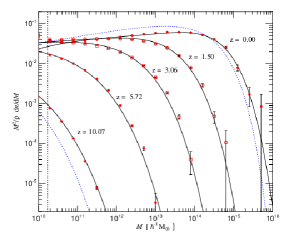
Figure 11: DM-halo mass function as a function of mass and redshift obtained by numerical simulations (Springel et al., 2005). The ordinate is the differential number density ($dn/dM$) multiplied by $M^{2}\rho^{-1}$ where $\rho$ is the mean density of the universe. The solid lines are the best-fit functions to the mass functions with the analytical functional form of Jenkins et al. (2001) (see also Sheth & Tormen 1999). The blue dashed lines are the Press-Schechter functions at $z=10.07$ and $0$ from left to right. This figure is reproduced by permission of the Nature Publishing Group.

Figure 12: Cosmic structures including DM halos reproduced by the state-of-the-art simulations (Ishiyama et al., 2015). From top to bottom, cosmic structures at $z=7$, $3$, $1$, and $0$ are shown. The left, center, and right panels represent the simulation results with three different DM-particle masses (box sizes), $2.2\times 10^{8}h^{-1}M_{\odot}$ ($1120h^{-1}$ Mpc), $2.8\times 10^{7}h^{-1}M_{\odot}$ ($140h^{-1}$ Mpc), and $3.4\times 10^{6}h^{-1}M_{\odot}$ ($70h^{-1}$ Mpc), respectively. This figure is reproduced by permission of the ASJ.

The DM halo formation is understood not only by numerical simulations, but also by analytic calculations. Starting from the Gaussian initial density fluctuations, one can derive an approximation of the DM-halo mass function based on linear structure growth and spherical collapse. The analytic form is referred to as the Press-Schechter function (Press & Schechter, 1974) that is,

$$n(M)dM=\frac{2}{\pi}\frac{a\rho_{0}}{{M^{*}}^{2}}\left(\frac{M}{M^{*}}\right)^{a-2}\exp\left[-\left(\frac{M}{M^{*}}\right)^{2a}\right]dM$$ (1)

where $M^{*}$ is the characteristic mass, $a$ is a power-law index of the mass fluctuations, and $\rho_{0}$ is the mean density of the universe. Figure 11 compares Press-Schechter functions (blue dashed lines) with numerical results (red points). The Press-Schechter functions reasonably approximate the numerical results, while there exist small departures. Note that theorists modify the analytic form of eq. (1), with a few additional free parameters (e.g. Sheth & Tormen 1999), and obtain ’modified’ Press-Schechter functions with the best-fit parameters determined by fitting the numerical results (solid lines in Figure 11). A number of galaxy formation studies (including LAE modeling) exploit such modified Press-Schechter functions that are useful to reproduce DM-halo mass functions (mass vs. abundance) at any redshifts and cosmological parameter sets (Mao et al., 2007; Samui et al., 2009). It should be also noted that these analytic formalisms can also provide reliable predictions in clustering of DM halos. In other words, once a redshift, mass, and cosmological parameter set are given, the abundance and clustering of DM halos are predicted by these formalisms based on the $\Lambda$CDM structure formation scenario.

Because galaxies form in DM halos, galaxy luminosity functions and stellar-mass functions should have a functional shape similar to DM halo mass functions. Indeed, galaxy luminosity functions determined by observations can be fit well with the Schechter function (Schechter, 1976),

$$\phi(L)dL=\phi^{*}\left(\frac{L}{L^{*}}\right)^{\alpha}\exp\left(-\frac{L}{L^{*}}\right)d\left(\frac{L}{L^{*}}\right)$$ (2)

where $\phi(L)$ is the number density of galaxies at luminosity $L$ . The Schuchter function includes three free parameters, $\phi^{*}$, $L^{*}$, and $\alpha$, that correspond to the characteristic number density, the characteristic luminosity, and the faint-end slope, respectively. Similarly, stellar mass functions are expressed with stellar mass $M_{\rm s}$ and the characteristic stellar mass $M_{\rm s}^{*}$ that are in place of $L$ and $L^{*}$, respectively, in Equation (2) (Figure 14).

It should be noted that Equation (2) has a functional form of the product of an exponential cut-off and a power law for luminosity, which is the same as Equation (1) where halo mass is replaced with luminosity.

The three free parameters of the Schechter function reflect differences from the DM-halo mass function, which depend on the baryonic processes of star-formation and feedback in galaxy formation (Section 2.1). In LAE studies, the Schechter function is used to approximate the Ly$\alpha$ luminosity function and the continuum luminosity function.

Star Formation

Star formation involves complicated physical processes of gas cooling and feedback as detailed below. Moreover, star-formation is induced by objects and matter outside of the galaxy by mergers and gas accretion. I choose gas cooling, feedback, and cold accretion that are key for understanding LAEs in the context of galaxy formation, and introduce these physical processes below.

Gas Cooling :

Star formation requires a reservoir of cold dense gas in a DM halo. However, such cold dense gas cannot be easily produced in a DM halo. If an adiabatic gas contraction takes place in the DM halo, gas temperature increases. Then, the gas contraction stops by the thermal pressure, and dense gas cannot be produced. In this way, adiabatic contractions do not make dense gas that is necessary for star formation. Star-formation thus requires a gas contraction associated with radiative cooling that reduces thermal energy in the gas cloud (Figure 10). By the radiative cooling, gas temperature should decrease from the virial temperature $T$ of the DM halo ($\mathrel{\hbox{\hbox to0.0pt{\hbox{\lower 4.0pt\hbox{$\sim$}}\hss}\hbox{$>$}}}10^{4}$ K) to the temperature of molecular hydrogen H₂ clouds ($\mathrel{\hbox{\hbox to0.0pt{\hbox{\lower 4.0pt\hbox{$\sim$}}\hss}\hbox{$<$}}}10^{2}$ K).

State-of-the-art simulations calculate the gas cooling processes numerically under realistic physical conditions, although these calculations cannot be described with simple analytical forms. Instead, I introduce a classic picture of gas cooling with the free-fall time of the spherical model (Silk & Wyse, 1993) that helps the readers understand the idea of gas cooling.

The cooling function, $\Lambda(T)$, is defined by

$$|\dot{E}_{\rm cool}|=n^{2}\Lambda(T),$$ (3)

where $\dot{E}_{\rm cool}$ and $n$ are the cooling rate (energy density divided by time) and the number density of particles, respectively. The cooling function is calculated based on quantum physics, and displayed in Figure 13. It is clear that metal rich gas has a higher $\Lambda(T)$, because various atomic electron transitions are allowed for heavy elements that enhance the efficiency of radiative cooling. In zero-metal gas, there are two peaks in $\Lambda(T)$ near $10^{4}$ and $10^{5}$ K that correspond to hydrogen and helium recombinations, respectively. The upturn of $\Lambda(T)$ from $10^{6}$ to $10^{8}$ K is explained by the cooling processes of Bremsstrahlung and Compton scattering.

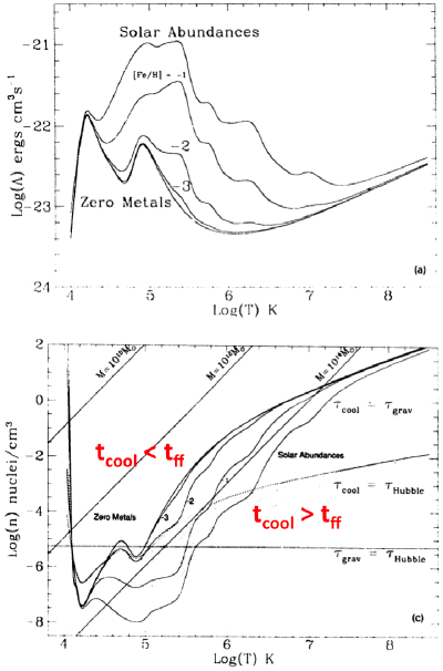
Figure 13: Cooling function (top) and gas density (bottom) as a function of virial temperature in a spherical halo (Silk & Wyse, 1993). Top: The curves represent cooling functions with various metal abundances from zero to one solar metallicities that are indicated by the labels. Bottom: The solid curves denote $t_{\rm cool}=t_{\rm ff}$ for the metal abundances from zero to one solar metallicities (same labels as in the top panel). Beyond these curves, the cooling time is shorter than the free-fall time, and gas collapses with a negligible thermal pressure. The dashed curve (the horizontal line) indicates that the cooling time (free-fall time) is equal to the present Hubble time. Above the curve and the horizontal line, the gas contraction completes in the cosmic time. The diagonal lines show the density and virial temperature that correspond to the virial masses of the system, $10^{10}$, $10^{12}$, and $10^{14}M_{\odot}$. This figure is reproduced by permission of the Physics Reports.

In a virialized system, the kinetic energy $E_{K}$ of gas is given by $E_{K}=3nk_{B}T/2$, where $k_{B}$ is the Boltzmann constant. Thus, the cooling time $t_{\rm cool}$ is given by

$$t_{\rm cool}=\frac{E_{K}}{|\dot{E}_{\rm cool}|}=\frac{3}{2}\frac{k_{B}T}{n\Lambda(T)}.$$ (4)

In the spherical model, the free-fall time $t_{\rm ff}$, a simple dynamical time, is

$$t_{\rm ff}=\sqrt{\frac{3\pi}{32G\rho_{\rm m}}},$$ (5)

where $\rho_{\rm m}$ is the mass density that is proportional to $n$. If the radiative cooling is very efficient, the cooling time is shorter than the free-fall time, $t_{\rm cool}<t_{\rm ff}$. In this case, gas collapse takes place with a negligible thermal pressure, and cold dense gas necessary for star formation is produced. This condition of $t_{\rm cool}<t_{\rm ff}$ for gas collapse is presented in the $T$ and $n$ plot of Figure 13 (bottom). Halo masses of $\sim 10^{12}M_{\odot}$ allow gas collapse down to the low gas densities, indicating an efficient gas cooling. It should be noted that the halo mass of $10^{12}M_{\odot}$ coincides with the mass of the Milky Way as well as the mass where the stellar-to-halo mass ratio is highest (Behroozi et al., 2013). Metals ease the conditions of gas collapse in a massive halo with $>10^{12}M_{\odot}$. In Figure 13, gas halos with $t_{\rm cool}>t_{\rm ff}$ cannot collapse but cause a quasi-static contraction due to inefficient cooling, which can take time longer than the Hubble time. As shown in Section 3.8, typical LAEs have halo masses of $10^{10}-10^{12}M_{\odot}$ and sub-solar metallicities. Figure 13 indicates that LAEs have physical parameters reasonably good for gas collapse, which enables subsequent star formation.

Feedback :

Feedback is known as one of the most important physical processes involved in star formation. Figure 14 compares an observed galaxy stellar-mass function (filled squares) with a DM halo mass function from numerical simulations (dashed line). Because the cosmic baryon fraction $f_{\rm b}$ is $f_{b}\equiv\Omega_{\rm b}/\Omega_{\rm m}\simeq 0.16$ (Planck Collaboration et al., 2015), the DM-halo mass function should be at least about an order of magnitude higher than the stellar-mass function, which can be clearly seen at $\sim 10^{11}M_{\odot}$ in Figure 14 (see the mass values at a constant number density of $\log N/{\rm[Mpc^{3}M_{\odot}]}\sim-14$). However, in Figure 14, the stellar-mass function is flatter at the low-mass end and steeper at the massive end than the DM-halo mass function. These shape differences are thought to be made by feedback effects that suppress star-formation by gas heating and outflow associated with star-formation and AGN activities in a galaxy (Bower et al., 2006).

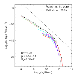
Figure 14: An observed baryonic (stars+cold gas) mass function of local galaxies (squares and the black dotted line; Bell et al. 2003) and the DM-halo mass function (dashed line; Weller et al. 2005). The colored solid and dotted lines indicate baryonic mass functions of various Hubble type galaxies: ellipticals, spirals, irregulars, and dwarf ellipticals. This figure is adopted from Read & Trentham (2005), and reproduced by permission of the Royal Society.

Theoretical studies assume two feedback mechanisms in the low and high mass regimes, energy- and momentum-driven feedback effects, respectively (Figure 15; Muratov et al. 2015). The energy-driven feedback for low-mass galaxies is caused by thermal energy inputs from supernova (SN) explosions and stellar radiation. The momentum-driven feedback for high-mass galaxies is activated by kinetic energy inputs from stellar winds, radiative pressure, and AGN jets. Defining the mass-loading factor $\eta\equiv\dot{M}_{\rm out}/SFR$ where $\dot{M}_{\rm out}$ is the outflow rate, numerical simulations show

$$\eta\propto V_{\rm circ}^{-2}$$ (6)

$$\eta\propto V_{\rm circ}^{-1}$$ (7)

for the energy and momentum driven feedbacks, respectively. Here, $V_{\rm circ}$ is the circular velocity given by

$$V_{\rm circ}=\sqrt{\frac{GM_{\rm h}}{r_{\rm vir}}},$$ (8)

where $M_{\rm h}$ and $r_{\rm vir}$ are the DM-halo mass and the virial radius, respectively. In Figure 15, the energy and momentum driven feedbacks are seen at $M_{\rm h}\mathrel{\hbox{\hbox to0.0pt{\hbox{\lower 4.0pt\hbox{$\sim$}}\hss}\hbox{$<$}}}10^{10}M_{\odot}$ and $\mathrel{\hbox{\hbox to0.0pt{\hbox{\lower 4.0pt\hbox{$\sim$}}\hss}\hbox{$>$}}}M_{\rm h}\sim 10^{10}M_{\odot}$, respectively. From observations of local galaxies, the relation of Equation (7) is confirmed (Heckman et al., 2015), while no observations reach $\mathrel{\hbox{\hbox to0.0pt{\hbox{\lower 4.0pt\hbox{$\sim$}}\hss}\hbox{$<$}}}M_{\rm h}\sim 10^{10}M_{\odot}$ to test the relation of the energy-driven feedback (Equation 6). Because the average DM-halo mass of LAEs is estimated to be $M_{\rm h}\sim 10^{11}M_{\odot}$ by clustering analysis (Section 3.8), feedbacks in typical LAEs are probably dominated by the momentum-driven feedback.

Note that some theoretical studies claim the existence of positive feedback effects that induce star-forming activities by, e.g., the shock cooling of AGN jets, radiation pressure, etc. (Silk, 2013; Vitale et al., 2015).

Figure 15: Mass loading factor as a function of $V_{\rm c}$ (left) and DM-halo mass (right) predicted by numerical simulations (Muratov et al., 2015). The red, blue, and black symbols represent galaxies at $z=0-0.5$ $(z_{\rm med}=0.25)$, $0.5-2$ $(1.25)$, and $2-4$ $(3)$, respectively, produced in the simulations. The red, blue, and black dotted lines indicate a broken-power law fit to the simulated galaxies at corresponding redshifts that roughly corresponds to the energy- and momentum-driven feedbacks (Equations 6 and 7), although the slope of the energy-driven feedback is slightly steeper than Equation (6). This figure is reproduced by permission of the the Royal Astronomical Society.

Cold Accretion :

Another important mechanism for star-formation is cold accretion. In the standard picture of galaxy growth, gas infalling in a DM halo is heated to a virial temperature by shocks at around the DM-halo virial radius, and then reaches a quasi-hydrostatic equilibrium with $T\sim 10^{6}(V_{\rm circ}/167$km s${}^{-1})^{2}$ K. The hot virialized gas cools by cooling radiation, and forms a cold gas disk that produces stars at the DM-halo center (Rees & Ostriker, 1977; White & Rees, 1978; Fall & Efstathiou, 1980). Recent theoretical studies suggest that, in this galaxy growth process, the infalling gas can penetrate into the DM halo center through the diffuse shock-heated medium, if the infalling gas is dense ($\sim 1$ cm^-3) and cold (a few $10^{4}$ K; Fardal et al. 2001; Kravtsov 2003; Kereš et al. 2005), which is referred to as cold accretion, cold mode accretion, or cold stream. The theoretical studies predict that, beyond the virial radius of DM halos, there exist multiple cold dense gas streams to the DM-halo center through filaments of LSSs (Figure 16). These cold dense gas streams collide at the DM-halo center, and cool very efficiently, which triggers intense star formation (Dekel et al., 2009). Such cold accretion is important, because about two-thirds of gas accretion in mass has a form of smooth gas flows, in contrast with the rest of the gas accretion taking place in a form of mergers with a $>1/10$-mass ratio (Katz et al., 2003; Kereš et al., 2009; Dekel et al., 2009)). This theoretical picture would explain high SFR galaxies with no merger signatures, such as bright LBGs and SMGs with an SFR of $\mathrel{\hbox{\hbox to0.0pt{\hbox{\lower 4.0pt\hbox{$\sim$}}\hss}\hbox{$>$}}}100M_{\odot}$ yr^-1, and could be an answer to the question why the number density of high SFR galaxies at $z\sim 2$ is significantly larger than those expected from merger events. Note that cold gas accretion is allowed in a massive halo only at $z\mathrel{\hbox{\hbox to0.0pt{\hbox{\lower 4.0pt\hbox{$\sim$}}\hss}\hbox{$>$}}}2$ (Figure 16), when the accretion gas is sufficiently cold.

Because the cold accretion is a theoretical picture, in the past decade observers have searched for a signature of cold accretion in their observational data. In LBGs at $z\sim 2$, velocities of low ionization metal absorption lines are mostly blueshifted from the galaxy systemic velocities, indicating gas outflow associated with star-forming activities (Steidel et al., 2010). Although there are several reports of cold accretion object candidates in deep observational studies (e.g. Nilsson et al. 2006; Rauch et al. 2011), no definitive observational evidence for cold accretion has been found so far. Because the cold accretion gas infalls along with filaments of LSSs, the covering fraction of cold accretion gas is very small, $\sim 1-2\%$ (Faucher-Giguère & Kereš, 2011). A large number of sightlines (i.e. a large sample of galaxies) would be needed to prove or disprove the existence of cold accretion.

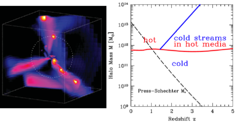
Figure 16: Left: Radial flux of cold gas accretion into the center of a DM-halo predicted by numerical simulations (Dekel et al., 2009). The color scale indicates the inflow rate per solid angle. The box size is 320 kpc. The dotted line represents the virial radius of the DM halo. There are three cold accretion streams clearly found in this figure, two of which include gas clumps with a mass ten times lower than that of the central galaxy. Right: DM-halo mass as a function of redshift (Dekel et al., 2009). The red horizontal curve indicates the threshold mass above which infalling gas is shock-heated around the DM-halo virial radius. The blue line represents the limit of cold accretion of gas whose density (temperature) is high (low) enough to penetrate into the DM halo center through the diffuse shock-heated medium. The dashed line denotes the characteristic DM-halo mass of the Press-Schechter mass function (eq. 1) at a given redshift. This figure is reproduced by permission of the Nature Publishing Group.

Role of Observations

As introduced in Section 2.1, the basic process of galaxy formation is DM-halo formation and star formation (Figure 10). DM-halo formation is well understood with no large systematics by simple numerical simulations and analytic approximations (Section 2.1), while star-formation is poorly understood due to the complicated baryonic processes: gas cooling, feedback, and cold accretion as well as merger induced star-formation. The star-formation process involves a number of unknown parameters, such as gas metallicity, density, temperature, outflow, and inflow. Observations can obtain these key parameters tightly connected to star formation, and constrain free parameters of galaxy formation models. On the other hand, many cosmological simulations including those for LAEs assume a simple relation between halo-mass and galaxy luminosity (e.g. McQuinn et al. 2007) as well as an empirical relation between gas and star-formation density such as the Kennicutt-Schmidt (KS) law (Figure 17). Such models with empirical relations can derive the star-formation surface density $\Sigma_{\rm SFR}$ from the gas surface density $\Sigma_{\rm gas}$ that is predicted by numerical simulations and semi-analytic models, and aim to explain other various observational quantities of galaxies (e.g. Garel et al. 2012). In this way, key observational parameters and empirical relations are important to understand star-formation in galaxies. Thus, the goal of observations is to determine star-formation key parameters and empirical relations to develop a self-consistent physical picture of galaxy formation

Figure 17: Star-formation surface density as a function of gas surface density (Kennicutt, 1998b). The gas surface density is defined by the average total surface density of atomic and molecular gas. The filled circles and squares represent normal-disk and starburst galaxies, respectively, in the local universe. The open circles denote the center of the normal-disk galaxies. The line is the least-squares fit to the data points, $\Sigma_{\rm SFR}\propto\Sigma_{\rm gas}^{1.4}$, which is known as the Kennicutt-Schmidt law. This figure is reproduced by permission of the AAS.

2.2 Origins of Ly$\alpha$ Emission from LAEs

Once a galaxy formation model is developed, Ly$\alpha$ emission of galaxies can be modeled. Theoretical studies suggest that in galaxies, Ly$\alpha$ emission can have five major origins, which probably explain the diversity of the spatial distribution of Ly$\alpha$ emission revealed by observations (Figure 18).

Ly$\alpha$ emission following hydrogen recombination in the ISM near the center of a galaxy can result from two origins of ionizing sources: i) star formation that makes Hii regions and ii) nuclear activities (i.e. AGN), if any, producing highly ionized broad and narrow-line regions in the galaxy center.

The remaining three origins are dominated by Ly$\alpha$ emission from the CGM to the outer halo: iii) outflowing gas that collisionally excites hydrogen whose Ly$\alpha$ to H$\alpha$ flux ratio is higher than the one of the optically thick case B recombination $f_{\rm Ly\alpha}/f_{\rm Ly\alpha}>8.7$ (Nakajima et al., 2013). iv) cooling radiation in the hot halo gas (Section 2.1), and v) fluorescence emission produced by the halo and IGM neutral hydrogen gas photo-ionized by UV background radiation supplied, e.g., by QSOs (Kollmeier et al., 2010).

Although Ly$\alpha$ emission can be made by these five photo-ionization and collisional excitation processes i)-v), Ly$\alpha$ photons experience resonance scattering in the Hi gas of the ISM, the CGM, and the IGM, due to the large Ly$\alpha$ cross section of Hi. Ly$\alpha$ photons are re-distributed in space and wavelength by the resonance scattering. For this reason, scattered Ly$\alpha$ emission would dominate in the CGM, where the Ly$\alpha$ intensity of photo-ionization is relatively weak. It should be noted that observations identify Ly$\alpha$ photons last scattered by Hi gas, and largely miss the original Ly$\alpha$ source position and gas dynamics information. However, this resonance nature of Ly$\alpha$ is also useful to probe the distribution and the kinematics of Hi gas by observations via theoretical modeling (Section 3.5).

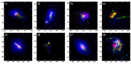
Figure 18: False-color images of local Ly$\alpha$ emitters obtained by the LARS survey (Hayes et al., 2013). The blue, red, and green colors indicate Ly$\alpha$ emission, H$\alpha$ emission, and far-UV continuum, respectively. The scales in units of kpc are shown in the vertical and horizontal axes. This figure is reproduced by permission of the AAS.

2.3 Summary of Galaxy Formation I

This section overviews the basic theoretical framework of galaxy formation and Ly$\alpha$ production, targeting young observers with a limited theoretical background. This section explains that galaxy formation is made of two physical processes of DM-halo formation and star formation. DM-halo formation is well understood with a simple robust model of cosmic structure formation consistent with observations. However, star formation involves complicated baryonic processes of gas cooling, feedback, and cold accretion as well as mergers that include many physical parameters difficult to determine. It is concluded that observations should constrain important physical parameters and empirical relations that are key for filling in the missing piece of the picture of galaxy formation. To understand LAEs in the context of galaxy formation, one also needs physical models of Ly$\alpha$ emission. Five Ly$\alpha$ emission origins in theoretical models are introduced. Two origins are in ISM regions: i) star formation (HII regions) and ii) AGN (highly-ionized gas in a galaxy center). The other three dominate in the CGM and outer halo regions: iii) outflowing gas, iv) cooling radiation, and v) fluorescence of UV background radiation. LAE observations should also reveal the origins of Ly$\alpha$ photons in parallel with the efforts to address the general galaxy formation issues.

3 Galaxy Formation II: LAEs Uncovered by Deep Observations

Since the discovery of LAEs in the late 1990s, various physical properties of LAEs have been revealed by exploiting deep optical to mid-infrared (MIR) imaging and spectroscopic capabilities of 8m-class ground based telescopes, HST, and Spitzer Space Telescope (Spitzer) in conjunction with observations at other wavelengths using the Chandra X-ray observatory (Chandra), GALEX, Herschel Space Observatory (Herschel), Atacama Large Millimeter / submillimeter Array (ALMA), and Very Large Array (VLA). In this section, I review key physical properties of LAEs uncovered by those observations: stellar population, luminosity function, morphology, ISM properties (metallicity, ionization parameter, dust), AGN activity, and clustering.

3.1 Stellar Population

The stellar population of galaxies is described by stellar mass, age, dust extinction, and some other parameters, and these parameters can be estimated by fitting broadband spectral energy distributions (SEDs) with stellar population synthesis models such as Bruzual & Charlot 2003. It is, however, difficult to investigate stellar populations of LAEs because most LAEs do not have detectable continuum emission even in deep images, although there do exist remarkably bright LAEs (Lai et al., 2008). Making a composite (average) SED of a number of continuum-faint LAEs by image stacking, early studies have revealed that they have faint and blue SEDs on average. An example SED is shown in the left panel of Figure 19 (Gawiser et al., 2007), which is explained by a model with a low stellar mass of $\sim 10^{9}M_{\odot}$, a young stellar age of $\sim 20$ Myr, and a negligibly small dust extinction.

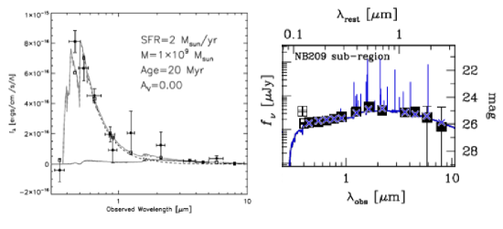
Figure 19: Left: A composite SED of LAEs at $z=3.1$ expressed in $f_{\lambda}$ (Gawiser et al., 2007). The thick solid line represents the best-fit SED that is made of an old (thin solid line) and young (dashed line) stellar components. Nebular emission is not included in modeling. Right: Same as the left panel, but for $z=2.2$ in $f_{\nu}$ (Nakajima et al., 2012). The blue line is the best-fit SED model that includes nebular emission. The blue crosses indicate the expected broadband photometry from the best-fit model. The two data points shown by open symbols are not used in the fitting in order to avoid a contamination from Ly$\alpha$ emission. This figure is reproduced by permission of the AAS.

Because LAEs are young dust-poor star-forming galaxies, they often have strong nebular lines, such as H$\alpha$, H$\beta$, [Oiii]5007, and [Oii]3727, which contaminate continuum fluxes estimated from broadband photometry. Because the observed-frame equivalent width $EW_{\rm obs}$ of nebular lines increases with redshift as $EW_{\rm obs}\propto(1+z)$, nebular lines of high-$z$ LAEs can cause serious systematic errors in broadband SEDs and hence in the calculation of stellar population parameters. Strong [Oiii], H$\beta$, and [Oii] lines near 4000Å mimic a Balmer break that is an indicator of stellar age, and an over/underestimated age leads to an over/underestimated stellar mass. Schaerer & de Barros (2009) introduce self-consistent population synthesis models with nebular lines where line ratios (as a function of metallicity) are fixed to the values of Galactic Hii regions. Using a sample of $z\sim 6$ LBGs as an example, they claim that models without nebular lines overestimate stellar ages and masses by a factor of $3$. Thus, considering nebular lines is critical to obtain stellar population parameters of high-$z$ young star-forming galaxies including LAEs. It should also be noted that there is another important source of contamination, nebular continuum, that is the free-free/bound-free emission of hydrogen and helium and two photon continuum emission of hydrogen. Because nebular continuum emission significantly changes UV-continuum colors for very young stellar populations with a stellar age of $\mathrel{\hbox{\hbox to0.0pt{\hbox{\lower 4.0pt\hbox{$\sim$}}\hss}\hbox{$<$}}}10$ Myr for instantaneous starbursts (see Figures 3 and 4 of Bouwens et al. 2010), it is usually included in nebular emission modeling.

The right panel of Figure 19 presents an average SED of $z=2$ LAEs and its best-fit stellar population synthesis model with nebular emission. Table 3.1 summarizes the typical ranges of stellar population parameters of $z=2-7$ LAEs that are obtained under the assumptions of constant star-formation history, a Salpeter IMF (Salpeter, 1955), and Calzetti extinction law (Calzetti et al. 2000; see Gawiser et al. 2007; Ono et al. 2010a, b; Guaita et al. 2011; Hagen et al. 2014, 2016). Although different samples give different parameter values, Table 3.1 shows that LAEs are low-stellar mass galaxies with a low dust extinction, a medium-low SFR, and a young stellar age.

Figure 20 compares LAEs (blue circles) with other galaxies in the stellar mass vs. SFR plane. At $M_{\rm s}\mathrel{\hbox{\hbox to0.0pt{\hbox{\lower 4.0pt\hbox{$\sim$}}\hss}\hbox{$>$}}}10^{10}M_{\odot}$ in Figure 20, there is a star-formation (SF) main sequence, a tight positive correlation between $M_{\rm s}$ and SFR (Daddi et al., 2007; Elbaz et al., 2007). LAEs fall in the low mass regime of $M_{\rm s}\sim 10^{7}-10^{10}M_{\odot}$ slightly above an extrapolation of the SF main sequence found at $M\mathrel{\hbox{\hbox to0.0pt{\hbox{\lower 4.0pt\hbox{$\sim$}}\hss}\hbox{$>$}}}10^{10}M_{\odot}$ (Hagen et al., 2014, 2016), suggesting that typical LAEs are high-$z$ dwarf galaxies in a weak burst mode. LAEs are located in a similar area in the stellar mass vs. SFR plane to other emission line galaxies, i.e., [Oii], H$\beta$, and [Oiii] emitters, at $z\sim 2$ (green dots).

Table 1: General Properties of Typical LAEs^†

Stellar Mass	$E(B-V)_{\rm s}$ a	SFR	Stellar Age	Metallicity
$[M_{\odot}]$		$[M_{\odot}$ yr${}^{-1}]$	$[$Myr$]$	$Z_{\odot}$
$10^{7}-10^{10}$	$0-0.2$	$1-100$	$1-100$	$0.1-0.5$

^a Color excess due to stellar extinction. The color excess due to nebular extinction, $E(B-V)_{\rm neb}$, falls in the same range as $E(B-V)_{\rm s}$ (Section 3.4). Calzetti’s extinction law (Calzetti et al., 2000) is assumed. ^† LAEs at $z\sim 2-3$ with a Ly$\alpha$ luminosity near $L^{*}_{\rm Ly\alpha}$, $\simeq 10^{42}-10^{43}$ erg s^-1.

Figure 20: LAEs compared with the star-formation main sequence on the SFR vs. stellar mass plot (Hagen et al., 2016). The blue circles represent LAEs, while the green circles denote optical emission galaxies (oELGs). The gray and magenta circles indicate BzK and Herschel/PACS-detected galaxies, respectively (Rodighiero et al., 2011). The dotted and dashed lines show the star-formation main sequences at $z=2$ obtained by Speagle et al. (2014) and Whitaker et al. (2014), respectively. This figure is reproduced by permission of the AAS.

3.2 Luminosity Function

The luminosity function and its evolution over time is one of the most fundamental properties for any galaxy population. The Ly$\alpha$ luminosity function of LAEs has been derived at $z\sim 0-8$ by large survey programs (Section 1.1) since the discovery of LAEs in the late 1990s. The bottom and top panels of Figure 21 present Ly$\alpha$ luminosity functions and their best-fit Schechter function parameters, respectively, from $z\sim 0$ to $6$, where the Schechter function parameters are the characteristic Ly$\alpha$ luminosity $L_{\rm Ly\alpha}^{*}$ and the normalization $\phi_{\rm Ly\alpha}^{*}$ that determines the abundance . Two evolutionary trends are seen in Figure 21: a monotonic increase in the normalization from $z\sim 0$ to $3$ and no evolution in either the normalization or the shape over $z\sim 3-6$. I explain details of these two trends in the following paragraphs.

Figure 21: Top: Best-fit Schechter parameters and the error contours of Ly$\alpha$ luminosity functions at $z\sim 0-6$ (Konno et al., 2016). The pluses represent the best-fit values while the contours indicate their 68% and 90% confidence levels. Redshift is coded by color: orange, $z=0.3$; magenta, 0.9; red, 2.2; blue, 3.1; cyan, 3.7; green, 5.7. Bottom: Ly$\alpha$ luminosity functions at $z\sim 0-6$ (Konno et al., 2016). The curves indicate the best-fit Ly$\alpha$ luminosity functions, with the same color code as the top panel. The red and blue circles show the data points of the Ly$\alpha$ luminosity functions at $z=2.2$ and $3.1$, respectively. This figure is reproduced by permission of the AAS.

The first evolutionary trend is an increase found at $z\sim 0-3$ (Deharveng et al., 2008; Cowie et al., 2010). It is notable that the abundance of $z=0.3$ LAEs is very low with $\phi_{\rm Ly\alpha}^{*}=1\times 10^{-4}$ Mpc^-3, about $50$ times lower than that of $z\sim 0$ SDSS optical-continuum selected galaxies, $\phi^{*}=5\times 10^{-3}$ Mpc^-3 (Blanton et al., 2001), meaning that LAEs are very rare in the local universe (Deharveng et al., 2008). The top panel of Figure 21 suggests that over $z=0.3$ and $z=2.2$ the increase is statistically more significant in Ly$\alpha$ luminosity ($L_{\rm Ly\alpha}^{*}$) than in the normalization ($\phi_{\rm Ly\alpha}^{*}$). The evolution of the Ly$\alpha$ luminosity function is also quantified with the Ly$\alpha$ luminosity density,

$$\rho_{\rm Ly\alpha}=\int^{\infty}_{L_{\rm Ly\alpha}^{\rm lim}}L_{\rm Ly\alpha}\phi_{\rm Ly\alpha}(L_{\rm Ly\alpha})dL_{\rm Ly\alpha},$$ (9)

where $L_{\rm Ly\alpha}$ and $L_{\rm Ly\alpha}^{\rm lim}$ are the Ly$\alpha$ luminosity and the limiting Ly$\alpha$ luminosity, respectively. For reference, the UV continuum luminosity density $\rho_{\rm UV}$ is defined by

$$\rho_{\rm UV}=\int^{\infty}_{L_{\rm UV}^{\rm lim}}L_{\rm UV}\phi_{\rm UV}(L_{\rm UV})dL_{\rm UV},$$ (10)

where $\phi_{\rm UV}(L_{\rm UV})$, $L_{\rm UV}$, and $L_{\rm UV}^{\rm lim}$ are the UV-continuum luminosity function, the UV-continuum luminosity, and the limiting UV-continuum luminosity, respectively. Figure 22 compares the evolutions of Ly$\alpha$ and UV-continuum luminosity densities, where the latter is derived with UV-continuum selected galaxies (Tresse et al., 2007). Figure 22 clearly shows that, from $z\sim 0$ to $3$, the Ly$\alpha$ luminosity density increases by a factor of $\sim 20-30$, which is significantly faster than the UV-continuum luminosity density evolution (a factor of $\sim 5-7$; Deharveng et al. 2008; Cowie et al. 2010). Similarly, in the same redshift range, the Ly$\alpha$ luminosity density increases even faster than the cosmic SFR density (a factor of $\sim 10$) on the Madau-Lilly plot (Madau & Dickinson, 2014), indicating that the Ly$\alpha$ luminosity density evolution cannot be explained by the cosmic SFR density evolution alone.

Figure 22: Ly$\alpha$-luminosity density (red triangles) and UV-continuum luminosity density (blue diamonds) as a function of redshift (Cowie et al., 2010). This figure is reproduced by permission of the AAS.

Figure 23: Left: Ly$\alpha$ emitting galaxy fraction $x_{\rm Ly\alpha}$ as a function of redshift (Stark et al., 2011). UV-continuum faint ($-20.25<M_{\rm UV}<-18.75$) and bright ($-21.75<M_{\rm UV}<-20.25$) galaxy results are shown in the top and the bottom panels. The red and blue circles (lines) represent the data points (the best-fit power law functions) for $EW_{0}>25$ Å galaxies with faint and bright UV-continuum magnitudes, respectively, while the purple and green squares (lines) are for $EW_{0}>55$ Å galaxies. The triangles with dashed error bars at $z\sim 7$ are predictions from the best-fit functions. Right: $x_{\rm Ly\alpha}$ as a function of UV-continuum magnitude for $EW_{0}>50$ Å galaxies at $z=3-6.2$ (Stark et al., 2010). The black circles represent measurements, while the red dashed line corresponds to the best-fit first-order polynomial to the data points. This figure is reproduced by permission of the AAS.

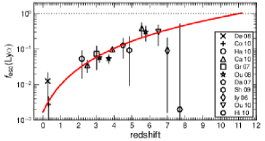
Figure 24: Average Ly$\alpha$ escape fraction as a function of redshift (Hayes et al., 2011a). The black symbols indicate average Ly$\alpha$ escape fraction estimates based on various observational results while the red line is the best-fit power law function to them. This figure is reproduced by permission of the AAS.

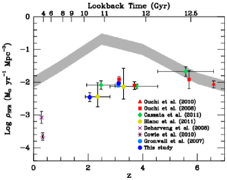
Figure 25: Cosmic SFR density as a function of redshift (Ciardullo et al., 2012). The data points with error bars represent the LAEs’ contribution to the cosmic SFR density, while the gray region indicates the total cosmic SFR density estimated with LBGs corrected for dust extinction. This figure is reproduced by permission of the AAS.

The second evolutionary trend is that the Ly$\alpha$ luminosity function is nearly constant over $z\sim 3-6$ (Ouchi et al., 2008). In contrast, the UV-continuum luminosity function of UV continuum-selected LBGs decreases from $z\sim 3$ to $6$ and beyond, indicating that Ly$\alpha$ emitting galaxies dominate in number more at $z\sim 6$ than at $z\sim 3$ (Ouchi et al., 2008). Indeed, deep spectroscopic surveys for UV-continuum selected LBGs suggest that the Ly$\alpha$ emitting (EW${}_{0}>25$Å) galaxy fraction $x_{\rm Ly\alpha}$ increases from $x_{\rm Ly\alpha}\sim 0.3$ to $0.5$ over $z=4-6$ for galaxies with an absolute UV magnitude $M_{\rm UV}$ range of $-20.25<M_{\rm UV}<-18.75$ corresponding to $\mathrel{\hbox{\hbox to0.0pt{\hbox{\lower 4.0pt\hbox{$\sim$}}\hss}\hbox{$<$}}}L_{\rm UV}^{*}$ (the left panel of Figure 23). In other words, about a half of $\mathrel{\hbox{\hbox to0.0pt{\hbox{\lower 4.0pt\hbox{$\sim$}}\hss}\hbox{$<$}}}L_{\rm UV}^{*}$-LBGs at $z\sim 6$ are LAEs with EW${}_{0}>25$ Å. This $x_{\rm Ly\alpha}$ evolution result indicates an increase with redshift in either the fraction of Ly$\alpha$ emitting galaxies or the Ly$\alpha$ luminosity of galaxies or both. Allowing both $\phi_{\rm Ly\alpha}^{*}$ and $L_{\rm Ly\alpha}^{*}$ to evolve, one can derive the number- and luminosity-weighted average Ly$\alpha$ escape fraction $\left<f_{\rm esc}^{\rm Ly\alpha}\right>$ from the Ly$\alpha$ luminosity density (Equation 9) as:

$$\left<f_{\rm esc}^{\rm Ly\alpha}\right>=\rho_{\rm Ly\alpha}/\rho_{\rm Ly\alpha}^{\rm int},$$ (11)

where $\rho_{\rm Ly\alpha}^{\rm int}$ is the intrinsic Ly$\alpha$ luminosity density expected from the cosmic SFR density $\Psi_{\rm SFR}$ (e.g. Madau & Dickinson 2014). The intrinsic Ly$\alpha$ luminosity density can be estimated by $\rho_{\rm Ly\alpha}^{\rm int}$ [erg s^-1 Mpc^-3] $=1.1\times 10^{42}\Psi_{\rm SFR}$ [$M_{\odot}$ yr^-1 Mpc^-3] under the assumption of the case B recombination ($L_{\rm Ly\alpha}/L_{\rm H\alpha}=8.7$; Brocklehurst 1971) and the H$\alpha$ luminosity $L_{\rm H\alpha}$-SFR relation of Kennicutt (1998a). Figure 24 presents $\left<f_{\rm esc}^{\rm Ly\alpha}\right>$ as a function of redshift (Hayes et al., 2011a), and indicates a monotonic increase in $\left<f_{\rm esc}^{\rm Ly\alpha}\right>$ from $z\sim 0$ to $6$.

Here I address the issue whether all of these observational results at $z\sim 3-6$ are self-consistent. Observations of UV-continuum selected galaxies show that faint UV-continuum galaxies have a higher chance of emitting strong Ly$\alpha$ in this redshift range (right panel of Figure 23; Ando et al. 2006; Stark et al. 2011). In other words, a majority of LAEs are faint UV-continuum galaxies. Although the abundance of bright ($>L^{*}$) UV-continuum galaxies drops significantly, the abundance of faint UV-continuum galaxies does not largely decrease towards high-$z$, due to a steepening of the luminosity function slope $\alpha$ (Bouwens et al., 2015). Because the abundance of LAEs is linked to the one of faint UV-continuum galaxies, the Ly$\alpha$ luminosity function of LAEs does not evolve largely over $z\sim 3-6$. In this way, all observational results suggest a self-consistent physical picture.

Because LAEs become a more dominant population at $z\sim 6$ than at $z\sim 3$, LAEs contribute much to the cosmic SFR density at $z\sim 6$. Figure 25 presents the evolution of the cosmic SFR density (Ciardullo et al., 2012). The contribution of LAEs is only $1/10$ of the total cosmic SFR density at $z\sim 3$ while it becomes the whole of it at $z\sim 6$. If this trend continues at $z\mathrel{\hbox{\hbox to0.0pt{\hbox{\lower 4.0pt\hbox{$\sim$}}\hss}\hbox{$>$}}}6$ (i.e. the EoR), LAEs may be a major population that emit ionizing photons for cosmic reionization. Thus, it is probably important to study LAEs to understand the physical properties of ionizing sources for cosmic reionization, although a large fraction of Ly$\alpha$ photons from LAEs (galaxies with intrinsically strong Ly$\alpha$ emission) may not reach observers due to absorption by neutral hydrogen in the IGM at the EoR (see Section LABEL:sec:cosmic_reionizationII for details of reionization sources).

An interesting approach to estimate the cosmic SFR density has been proposed by Croft et al. (2016). It is based on the so-called intensity mapping technique, and consists in determining the power spectrum of diffuse Ly$\alpha$ emission from star-forming galaxies that are too faint to be detected individually, but numerous enough to yield a significant signal in a statistical sense. Croft et al. (2016) have found that the cosmic SFR density at $z=2-3.5$ estimated from diffuse Ly$\alpha$ emission is about 30 times higher than those by Ciardullo et al. (2012) and comparable to (or higher than) the dust-extinction corrected total cosmic SFR density. Because some amount of Ly$\alpha$ emission should be absorbed by dust, this result may be overestimating the true cosmic SFR density. Although being a powerful important technique, intensity mapping requires a very careful evaluation of systematics. Recently, Croft et al. (2018) have updated the analysis with the systematics removals, reducing the intensity measurement of the diffuse Ly$\alpha$ emission by a factor of 2. Croft et al. (2018) find that there is no correlation between the diffuse Ly$\alpha$ emission and the Ly$\alpha$ forest, and show that the diffuse Ly$\alpha$ emission is not explained by faint star-forming galaxies, but fluorescence Ly$\alpha$ emission around QSOs in a scale up to $15h^{-1}$ Mpc.

3.3 Morphology

It has been known that LAEs are generally very compact since first revealed by HST in the mid 90’s (Pascarelle et al. 1996a, b; Figure 26). Deep HST images reveal small effective radii, $r_{\rm e}$, in rest-frame UV and optical continua, $\sim 1$ kpc on average (Malhotra et al., 2012; Paulino-Afonso et al., 2018; Shibuya et al., 2018c). The radial profiles of the rest-frame UV and optical continua typically show a disk morphology with a Sérsic index $n$ of $n\simeq 1$, and follow the $r_{\rm e}$-magnitude relation similar to the one of LBGs, indicating that faint continuum LAEs have a small size in $r_{\rm e}$ (Figure 27; Paulino-Afonso et al. 2018; Shibuya et al. 2018c). Because a majority of LAEs have a faint continuum, the $r_{\rm e}$-magnitude relation can explain the compact morphologies of LAEs.

Although previous HST studies claim no redshift evolution of $r_{\rm e}$ on average, a recent HST study (Shibuya et al., 2018c) finds that the no-redshift evolution results may be produced by the sample selection bias. If a sample selection is not controlled, one can identify more LAEs with a faint continuum at low redshift. Because LAEs with a faint continuum have a $r_{\rm e}$ value smaller than LAEs with a bright continuum due to the $r_{\rm e}$-magnitude relation, $r_{\rm e}$ measurements of low-redshift LAEs are typically small, diminishing the trend of the redshift evolution. Figure 28 shows the median $r_{\rm e}$ value as a function of redshift that is obtained with the controlled samples whose LAEs fall in the same continuum luminosity range (Shibuya et al., 2018c). The median $r_{\rm e}$ value monotonically decreases as $\sim(1+z)^{-1}$ for a given continuum luminosity (Shibuya et al., 2018c). This evolutionary trend of LAEs is similar to the one of LBGs (e.g. Shibuya et al. 2015).

The compact morphology of LAEs is not only found in continua, but also in Ly$\alpha$ emission by HST narrowband imaging studies (Bond et al., 2010; Finkelstein et al., 2011b). It should be noted that deeper narrowband-imaging and spectroscopic observations identify very diffuse extended ($\mathrel{\hbox{\hbox to0.0pt{\hbox{\lower 4.0pt\hbox{$\sim$}}\hss}\hbox{$>$}}}10$ kpc) Ly$\alpha$ halos around LAEs that are detailed in Section LABEL:sec:galaxy_formationIII (Hayashino et al., 2004; Steidel et al., 2011; Patrício et al., 2016; Wisotzki et al., 2016). A combination of these observational studies indicates that the spatial structure of Ly$\alpha$ emission of LAEs is composed of a peaky Ly$\alpha$ core and a diffuse Ly$\alpha$ halo (see also Leclercq et al. 2017)

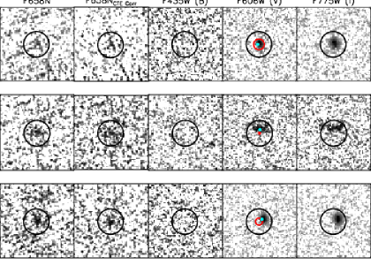
Figure 26: HST images of three LAEs dubbed CHa-2, CH8-1, and CH8-2 at $z=4.4$ (Finkelstein et al., 2011b): from left to right, narrowband $F658N$, narrowband $F658N$ corrected for the charge-transfer effect, $B_{435}$, $V_{606}$, and $i_{775}$. The $F658N$ band includes the redshifted Ly$\alpha$ emission of the LAEs. The centers of the black circles indicate the centroids of the LAEs in the $F658N$ band. See Finkelstein et al. (2011b) for more details. This figure is reproduced by permission of the AAS.

Figure 27: Left: Radial profile of UV-continuum surface brightness obtained with the HST images (Shibuya et al., 2018c). The red shade represents the radial profile of the composite LAE with the $1\sigma$ uncertainty. The composite LAE consists of LAEs with $0.12-1L^{*}_{\rm z=3}$ at $z=0-7$, where $L^{*}_{\rm z=3}$ is the characteristic luminosity of the Schechter function for the UV luminosity function at $z=3$. The black solid and dashed lines indicate the Sérsic profiles with $n=1$ and $4$, respectively. The gray line denotes the radial profile of the point-spread function (PSF). Right: Size-magnitude ($r_{\rm e}$-magnitude) relation (Shibuya et al., 2018c). The top two panels show the size-magnitude relations in the rest-frame optical wavelength, while the bottom two panels present those in the rest-frame UV wavelength. The red and cyan circles represent LAEs and continuum-selected star-forming galaxies, respectively, where the error bars indicate the 16th- and 84th-percentiles of the $r_{\rm e}$ distribution. The red dots indicate the size and magnitude measurements of individual LAEs. The cyan dotted lines are the power law functions best fit to the data points of the cyan circles. The gray symbols represent the measurements for LAEs obtained in the other studies. This figure is reproduced by permission of the AAS.

Figure 28: Effective radius as a function of redshift for LAEs and LBGs with the same UV-continuum luminosity of $0.12-1\ L^{*}_{\rm z=3}$ (Shibuya et al., 2018c). Here, $L^{*}_{\rm z=3}$ is the characteristic luminosity of the Schechter function for the UV luminosity function at $z=3$. The red filled diamonds (with the black circle) indicate LAEs in the rest-frame UV (optical) wavelength. The red open diamond at $z\sim 0.5$ ($z\sim 7.5$) represents the effective radius in the rest-frame optical (UV) wavelength estimated from the extrapolation of the size-magnitude relation (the small sample consisting of 3 LAEs). The small and large cyan circles denote the effective radii of galaxies selected by photo-$z$ and Lyman break techniques, respectively. The red-broad and cyan-dashed curves show the power-law functions of $(1+z)^{\beta}$ for $\beta\simeq-1$ that are best-fit to the data points of the red filled diamonds and the cyan filled circles, respectively. The gray and black symbols present the effective radii obtained by various studies whose magnitude limits are different. This figure is reproduced by permission of the AAS.

3.4 ISM Properties

Hydrogen in the ISM has three gas phases: H⁺ ions, H atoms, and H₂ molecules. Corresponding to these three phases, the ISM is classified into three regions: Hii regions (H⁺), photodissociation regions (PDR; H), and molecular regions (H₂) whose gas temperatures are $\sim 10^{4}$, $10^{2}-10^{3}$, and $10^{1}-10^{2}$ K, respectively (Figure 29).

Figure 29: Top: Hydrogen density as a function of visual extinction $A_{\rm V}$ that corresponds to the illuminated face (small $A_{\rm V}$) to the shielded face (large $A_{\rm V}$; Abel et al. 2005). The dashed, dotted, and solid curves represent the model predictions of the ionized, atomic, and molecular hydrogen densities, respectively. The two vertical lines indicate the hydrogen ionization front and the half-density molecular hydrogen point. Bottom: Predicted gas temperature as a function of $A_{\rm V}$. This figure is reproduced by permission of the AAS.

In local galaxies, most of the ISM is in PDRs, where UV radiation from stars photodissociates molecules. However, PDRs have large spatial variations of temperature and density (Figure 29), making it difficult to understand PDR properties by simple modeling. Moreover, there are many atomic and molecular transitions in PDRs as well as in molecular regions. In contrast, Hii regions are moderately homogeneous media with a small number of ionization transitions, and thus can be modeled more simply than PDRs and molecular regions. It should also be noted that Hii regions radiate emission lines falling in optical wavelengths where ground-based deep spectroscopy is possible. These emission lines enable us to constrain physical parameters of Hii regions such as gas-phase metallicity, electron temperature $T_{\rm e}$, ionization parameter $q_{\rm ion}$, and electron density $n_{\rm e}$.

Although it is difficult to characterize ISM properties of LAEs that are generally faint, recent LAE observations have constrained the gas-phase metallicity and ionization parameter in Hii regions. Moreover, there are some useful observations to constrain parameters of atomic gas and dust mainly found in PDRs and molecular regions. Below I explain observational results as well as the methods used to probe the ISM properties.

Gas-Phase Metallicity

One of the most important ISM quantities that characterize galaxies is the gas-phase metallicity of Hii regions. The metallicity of a galaxy is estimated from the ratio of appropriate lines using photoionization models. Depending on the strength of the lines used, there are two methods: the direct $T_{\rm e}$ method and the strong emission line method. Note that all of the line ratios discussed below are corrected for dust extinction.

Direct $T_{\rm e}$ Method

The direct $T_{\rm e}$ method mainly uses weak lines sensitive to electron temperature, Oiii]1661,1666, [Oiii]4363, [Nii]5755, and [Oii]7320,7330 etc. Because the most popular line among these is the auroral [Oiii]4363 line, below I explain the direct $T_{\rm e}$ method with this line.

One can estimate $T_{\rm e}$ from [Oiii]4363 and [Oiii]4959,5007 line fluxes using the following equation:

$$(f_{[{\rm OIII}]4959}+f_{[{\rm OIII}]5007})/f_{[{\rm OIII}]4363}=\frac{7.90\exp(3.29\times 10^{4}/T_{\rm e})}{1+4.5\times 10^{-4}n_{\rm e}/T_{\rm e}^{1/2}},$$ (12)

with a small uncertainty depending on $n_{\rm e}$ (left panel of Figure 30; Osterbrock 1989). The $T_{\rm e}$ value is determined by the ratio $(f_{[{\rm OIII}]4959}+f_{[{\rm OIII}]5007})/f_{[{\rm OIII}]4363}$, because the [Oiii]4363 ([Oiii]4959,5007) flux increases (decreases) when the rate of collisional excitation (de-excitation) from ¹D₂ to ¹S₀ (from ¹D₂ to ³P) increases with $T_{\rm e}$ (right panel of Figure 30) .

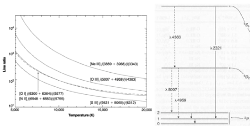
Figure 30: Left: Line ratios as a function of electron temperature (Osterbrock, 1989). The second top curve indicates the line ratio $(f_{[{\rm OIII}]4959}+f_{[{\rm OIII}]5007})/f_{[{\rm OIII}]4363}$, while the other curves show line ratios that are not discussed in the text. Right: Schematic diagram presenting the quantum states ¹S₀, ¹D₂, and ³P of an ${\rm O}^{2+}$ ion and emission lines produced by transitions between two states (Osterbrock, 1989). The solid and dashed-line arrows represent permitted and forbidden lines, respectively. This figure is reproduced by permission of the University Science Books.

Because metals are major coolants of the gas in Hii regions, $T_{\rm e}$ is primarily determined by metallicity. Therefore, if $T_{\rm e}$ is estimated, one can reliably derive the metallicity based on photoionization models (Izotov et al., 2006),

$$12+\log\frac{{\rm O}^{+}}{{\rm H}^{+}} = \log\frac{f_{[{\rm OII}]3727}}{f_{{\rm H}\beta}}+5.961+\frac{1.676}{t_{2}}$$ (13)

$$-0.40\log t_{2}-0.034t_{2}+\log(1+1.35x),$$

$$12+\log\frac{{\rm O}^{2+}}{{\rm H}^{+}} = \log\frac{f_{[{\rm OIII}]4959}+f_{[{\rm OIII}]5007}}{f_{{\rm H}\beta}}+6.200+\frac{1.251}{t_{3}}$$ (14)

$$-0.55\log t_{3}-0.014t_{3},$$

where

$$t_{2}=10^{-4}T_{\rm e}{\rm[OII]},$$ (15)

$$t_{3}=10^{-4}T_{\rm e}{\rm[OIII]},$$ (16)

$$x=10^{-4}n_{\rm e}t_{2}^{-0.5},$$ (17)

and ${\rm O}^{+}$, ${\rm O}^{2+}$, and ${\rm H}^{+}$ are the abundances of singly-ionized oxygen, doubly-ionized oxygen, and ionized hydrogen, respectively; $T_{\rm e}$[Oii] and $T_{\rm e}$[Oiii] are the electron temperatures in ${\rm O}^{+}$ and ${\rm O}^{2+}$ ion gas. For simplicity, one can assume the relation (Campbell et al., 1986; Garnett, 1992)

$$t_{2}=0.7t_{3}+0.3$$ (18)

that generally does not change the metallicity estimate. Because the last term of eq. (13), $\log(1+1.35x)$, is negligibly small, this term can be practically omitted.

The oxygen abundance is calculated with

$$\frac{{\rm O}}{{\rm H}}=\frac{{\rm O}^{+}}{{\rm H}^{+}}+\frac{{\rm O}^{2+}}{{\rm H}^{+}}.$$ (19)

It should be noted that the contribution of ${\rm O}^{3+}$ and higher-order ionized oxygen is negligibly small, only $<1$%, in Hii regions heated by stars.

Strong Emission Line Method

The strong emission line method uses flux ratios of major emission lines of star-forming galaxies that include [Oii]3727, H$\beta$4861, [Oiii]5007, H$\alpha$6563, and [Nii]6584. One of the most frequently used line ratios is the $R_{23}$ index defined by:

$$R_{23}=\frac{f_{\rm[OII]3727}+f_{\rm[OIII]4959}+f_{\rm[OIII]5007}}{f_{\rm H\beta}}.$$ (20)

The top panel of Figure 31 presents $R_{23}$ as a function of oxygen abundance. The solid lines in this panel show $R_{23}$-oxygen abundance relations calculated by photoionization models with different ionization parameter ($q_{\rm ion}$) values. Here, $q_{\rm ion}$ is defined by

$$q_{\rm ion}=\frac{Q_{\rm H^{0}}}{4\pi R_{\rm s}^{2}n_{\rm H}},$$ (21)

where $Q_{\rm H^{0}}$ is the number of hydrogen ionizing photons produced per unit time. $R_{\rm s}$ is the Str$\ddot{\rm o}$mgren radius, and $n_{H}$ is the hydrogen density. Because $R_{23}$ strongly depends on $q_{\rm ion}$ (see the top panel of Figure 31), one needs to empirically calibrate the $R_{23}$-oxygen abundance relation with local galaxies that have $R_{23}$ and oxygen abundance measurements from the direct $T_{\rm e}$ method. In the top panel of Figure 31, the star marks with error bars denote the average values of the local galaxies, and the dashed line is an empirical relation that fits the star marks. In this way, a locally calibrated empirical relation is used to derive oxygen abundances from $R_{23}$ measurements. However, it should be noted that the oxygen abundances of high-$z$ galaxies estimated in this manner have systematic errors because ISM properties of high-$z$ galaxies including $q_{\rm ion}$ are different from those of local galaxies (Nakajima & Ouchi, 2014).

Figure 31: $R23$ ($N2$) index as a function of oxygen abundance presented in the top (bottom) panel (Nagao et al., 2006). The star marks denote local galaxy averages obtained by the direct $T_{\rm e}$ method, and the dashed line represents an empirical fit to them. The solid lines show photoionization model calculation results with the normalized ionization parameter, $U\equiv q_{\rm ion}/c$, of $\log U=-3.8$, $-3.5$, $-3.2$, $-2.9$, $-2.6$, $-2.3$, and $-2.0$ from bottom to top (top to bottom) in the top (bottom) panel. The dotted lines indicate solar metallicity. This figure is reproduced by permission of the Astronomy & Astrophysics journal.

The top panel of Figure 31 shows a degeneracy in all $R_{23}$-oxygen abundance relations because there are basically two possible oxygen abundances for a given $R_{23}$ measurement. This is because $R_{23}$ increases with increasing metallicity up to $\sim 1Z_{\odot}$, while at higher metallicities fine-structure cooling emission in far-infrared (FIR) wavelengths dominates and reduces the collisionally excited line fluxes of [Oii] and [Oiii] that are the numerators of $R_{23}$. To resolve this degeneracy, one can use the $N2$ index defined by:

$$N2=\frac{f_{\rm[NII]6584}}{f_{\rm H\alpha}}.$$ (22)

The bottom panel of Figure 31 displays photoionization model calculations (solid lines), local galaxy averages (star marks), and an empirical $N2$-oxygen abundance relation that fits the local galaxy averages (dashed line). Since the $N2$ index does not include oxygen line measurements i.e. only $f_{\rm[NII]6584}$ and $f_{\rm H\alpha}$, oxygen abundances from the $N2$ index have a systematic uncertainty due to a possible variation of the nitrogen-to-oxygen abundance ratio, implying that the $N2$ index alone is not a good estimator of oxygen abundance. However, one can obtain a coarse oxygen abundance estimate from an $N2$ index (eq. 22) measurement that is useful to resolve the degeneracy of the $R_{23}$-oxygen abundance relation discussed above. Once the degeneracy is resolved by the $N2$ index, a single solution of oxygen abundance can be obtained from the $R_{23}$ index.

Because the strong emission line method does not use weak lines such as the [Oiii]4363 auroral line whose flux intensity is only $\sim 1/70$ of [Oiii]5007 (Izotov et al., 2006), it can efficiently estimate the metallicities of faint galaxies including LAEs. However, as described above, one should keep in mind that abundances based on the strong emission line method would be biased if the ISM properties of galaxies in question are different from those of local calibrators.

Metallicity Estimates of LAEs

Although it is difficult to determine the metallicity of LAEs due to their faintness, some constraints have been obtained for a small number of LAEs . Finkelstein et al. (2011a) have obtained upper limits of $Z<0.17Z_{\odot}$ and $<0.28Z_{\odot}$ for two LAEs with the spectroscopic $N2$ index (see also Guaita et al. 2013), while Nakajima et al. (2012) have placed a lower limit of $Z>0.09Z_{\odot}$ for a stack of 105 LAE narrowband images that cover [Oii]3727, [Nii]6584, and H$\alpha$ lines based on a combination of two strong line methods, the $N2$ index and the [Oii]/H$\beta$ index (Nagao et al., 2006). Nakajima & Ouchi (2014) have examined the metallicities of 6 LAEs at $z=2-3$ with the $R23$ index and the ratio of [Oiii]5007 to [Oii]3727 fluxes, and found that they fall in the range of $12+\log({\rm O/H})=7.98-8.81$,with an average of $Z\sim 0.5Z_{\odot}$. These metallicity constraints generally agree with the mass metallicity relation (Finkelstein et al., 2011a) and an extrapolation of the SFR-mass metallicity relation to low mass of star-forming galaxies at similar redshifts (Nakajima et al., 2012).

More recently, Kojima et al. (2017) have measured the oxygen abundances of LAEs by the direct $T_{\rm e}$ method (left panel of Figure 32), to show that one LAE (and five lensed LAEs) has (have) a metallicity (metallicity range) of $Z=0.26^{+0.08}_{-0.07}Z_{\odot}$ ($Z=0.1-0.3Z_{\odot}$). The right panel of Figure 32 presents oxygen abundance and ionization parameter measurements for the one LAE and four lensed LAEs, after carefully removing one lensed LAE (ID 6) whose value, $Z=0.1Z_{\odot}$, is based on unreliable flux estimates. These results by the direct $T_{\rm e}$ method and the strong line method suggest that the gas-phase metallicity of LAEs at $z\sim 2-3$ is typically $Z\simeq 0.1-0.5Z_{\odot}$ (Table 3.1). So far, no extremely metal poor LAEs with $Z\mathrel{\hbox{\hbox to0.0pt{\hbox{\lower 4.0pt\hbox{$\sim$}}\hss}\hbox{$<$}}}0.01Z_{\odot}$ have been identified. However, because most of the LAEs with metallicity estimates are moderately bright, there remains a possibility that very metal poor LAEs are found in future studies targeting faint objects.

Figure 32: Left: Electron temperature as a function of stellar mass (Kojima et al., 2017). The red filled/open squares marked with a black open square are one un-lensed LAE (ID 1) and five lensed LAEs (IDs 3, 4, 5, 6, and 11). Note that ID 6 does not have reliable line flux estimates. The other squares and the star mark indicate individually-identified LBGs and a stacked LBG, respectively. Right: Oxygen abundance and ionization parameter of LAEs and LBGs that are estimated by the reliable direct $T_{\rm e}$ method (Kojima et al., 2017). The red filled squares marked with a black square are LAEs (IDs 1, 3, 4, 5, and 11), where ID 6 with an unreliable result ($Z=0.1Z_{\odot}$) is removed. The blue star mark indicates the stacked LBG. The black circles denote the results of local galaxy stacks, while the black line (the gray region) represents the local best-fit power law relation between oxygen abundance and ionization parameter (the typical scatter around the best-fit power law). This figure is reproduced by permission of the PASJ.

Figure 33: Left: $O_{32}$ $(=f_{\rm[OIII]5007}/f_{\rm[OII]3727})$ as a function of $R_{23}$ (Nakajima & Ouchi, 2014). The Red and blue diamonds indicate LAEs and LBGs, respectively, at $z=2-3$. The green circles, magenta circles, and orange pentagons denote, respectively, green-pea galaxies, Lyman-break analogs, and Lyman continuum leaking galaxies in the local universe. The gray triangles and dots represent $z\sim 1$ galaxies and $z\sim 0$ SDSS galaxies, respectively. The three solid lines show photoionization model tracks with the ionization parameter of $q_{\rm ion}=3\times 10^{8}$, $8\times 10^{7}$, and $2\times 10^{7}$ cm s^-1 from top to bottom. The model tracks cover the oxygen abundance, from $12+\log({\rm O/H})=7.5$ to $9.0$ and beyond, with dotted lines connecting the same oxygen abundances. Right: Schematic illustrations of two types of Hii regions: (a) an ionization bounded nebula and (b) a density-bounded nebula (Nakajima & Ouchi, 2014). The blue and gray regions denote Hii and Hi gas regions, respectively. The star marks represent massive stars emitting ionizing photons. The cyan solid (dotted) lines indicate the (expected) positions of the Str$\ddot{\rm o}$mgren radius. This figure is reproduced by permission of the AAS.

Figure 34: Left: Ciii]1909 rest-frame equivalent width as a function of Ly$\alpha$ rest-frame equivalent width (Stark et al., 2015a). The red stars, orange circles, black triangles, and blue squares represent galaxies including LAEs at $z=6-7$, $1.5-3.0$, $2.3$, and $3$, respectively. Right: [Cii]158$\mu$m luminosity as a function of SFR (Knudsen et al., 2016). The cyan diamond/circles, purple circles, orange circles, green circles, and black squares indicate LAEs. The blue and red circles are continuum-bright LBGs, some of which show Ly$\alpha$ emission. This figure is reproduced by permission of MNRAS.

Figure 35: Left: Observed SED of EGS-zs8-2 at $z=7.48$ (red circles; Roberts-Borsani et al. 2016). The blue line denotes the best-fit SED model with nebular emission lines. The open diamonds are the expected photometry in the photometric bands for the best-fit SED. The vertical dashed lines mark the wavelengths of major nebular emission lines. The observed flux density at $4.5\mu$m shows an excess that is probably made by strong [Oiii]4959,5007 and H$\beta$ line emission. Right: [Oiii]$88\mu$m (top) and Ly$\alpha$ lines of SXDF-NB1006-2 (Inoue et al., 2016). The dotted line denotes the $1\sigma$ noise level. The blue and purple dashed lines represent the line-peak velocities of [Oiii]$88\mu$m and Ly$\alpha$, respectively. The red curve in the top panel indicates the best-fit Gaussian function to the [Oiii]$88\mu$m line. The gray regions in the bottom panel show the wavelength range with large sky subtraction systematics. This figure is reproduced by permission of the AAS and Science.

Ionization State

The ionization state of typical LAEs’ Hii regions is clearly different from those of other types of high-$z$ galaxies. Recent optical-NIR spectroscopy has revealed that the $O_{32}$ ratios of $z\sim 2-3$ LBGs and LAEs are significantly higher than those of local SDSS galaxies (left panel of Figure 33; Nakajima et al. 2013; Nakajima & Ouchi 2014), where the $O_{32}$ ratio is defined by

$$O_{32}=\frac{f_{\rm[OIII]5007}}{f_{\rm[OII]3727}}.$$ (23)

Specifically, LAEs have extremely large values of $O_{32}\sim 10$, being about $\sim 10-100$ times higher than those of the local SDSS galaxies and even higher than those of the LBGs on average. In the left panel of Figure 33, photoionization models with various metallicity and $q_{\rm ion}$ values are compared with LAEs. Although the models predict that $O_{32}$ increases with decreasing metallicity, the high $O_{32}$ values of LAEs cannot be explained by models that reproduce the local SDSS galaxies with $q_{\rm ion}=0.1-1\times 10^{8}$ cm s^-1. The $z\sim 2-3$ LAEs are found to have $q_{\rm ion}=1-9\times 10^{8}$ cm s^-1, about an order of magnitude larger than those of the local SDSS galaxies (Nakajima & Ouchi, 2014). The left panel of Figure 33 also shows that there exist local counterparts to LAEs, green pea galaxies (GPs; Cardamone et al. 2009; Jaskot & Oey 2014), whose $O_{32}$ and $R_{23}$ values are comparable with those of LAEs.

The physical origin of the high $q_{\rm ion}$ values of LAEs is not well understood. The ionization parameter defined by eq. (21) is rewritten as

$$q_{\rm ion}^{3}\propto Q_{\rm H^{0}}n_{\rm H}\epsilon^{2}$$ (24)

by the substitution of the Str$\ddot{\rm o}$mgren radius. Here, the Str$\ddot{\rm o}$mgren radius $R_{\rm s}$ is defined as

$$Q_{\rm H^{0}}=\frac{4}{3}\pi R_{\rm s}^{3}n_{\rm H}^{2}\alpha_{\rm B}\epsilon$$ (25)

with the coefficient of the total hydrogen recombination to the $n>1$ levels $\alpha_{\rm B}$, where $\epsilon$ is the volume filling factor of the Str$\ddot{\rm o}$mgren sphere. Eq. (24) indicates that either $Q_{\rm H^{0}}$, $n_{\rm H}$, or $\epsilon$ needs to increase by a factor of $10^{3}$, $10^{3}$, or $30$, respectively, to explain the high $q_{\rm ion}$ values of LAEs. With a moderately high SFR and metal-poor young stellar population, LAEs produce ionizing photons more efficiently than the local SDSS galaxies. However, it may not be possible that the $Q_{\rm H^{0}}$ of LAEs are $\sim 10^{3}$ times higher than those of the local SDSS galaxies. Some studies have reported an increase in the electron density from $\sim 25$ cm^-3 ($z\sim 0$) to $\sim 250$ cm^-3 ($z\sim 2$; Steidel et al. 2014; Shimakawa et al. 2015; Sanders et al. 2016), but these increase rates are not as high as $10^{3}$ times. It is also unlikely that the average $\epsilon$ increases by a factor of 30 from $z\sim 0$ to $2$. I discuss the issue of high $q_{\rm ion}$ at the end of this subsection.

Some other observations also suggest that LAEs have high $q_{\rm ion}$ values. LAEs with a large Ly$\alpha$ $EW_{0}$ tend to have high-ionization metal lines in rest-frame UV spectra. Stark et al. (2014) have identified moderately strong Ciii]1901,1909 lines in lensed LAEs at $z\sim 2$ by deep spectroscopy, and revealed a positive correlation between Ly$\alpha$ and Ciii]1901,1909 $EW_{0}$. The left panel of Figure 34 suggests that high-ionization lines Ciii]1901,1909 are strong for large-Ly$\alpha$ $EW_{0}$ galaxies such as LAEs. Highly ionized gas containing C²⁺ is probably more abundant in LAEs compared to other types of galaxies. Subsequently, Stark et al. (2015a) and Stark et al. (2015b) have reported the detections of moderately strong lines of Ciii]1907,1909 lines in two LAEs at $z=6-7$ and Civ1548 line in an LAE at $z=7$, respectively. Although there still remains the possibility that the Civ1548 line is produced by a hidden AGN, not by young, massive stars (e.g. detection of Nv1239 for the definitive AGN identification; Laporte et al. 2017), these spectroscopic results suggest that ionization state of LAEs at $z=2-7$ is very high.

Most of the ALMA studies of LAEs have targeted the [Cii]158$\mu$m fine structure line that originates from low-ionization C⁺ gas. Because C has a lower ionization potential than H, it is thought that the majority of [Cii]158$\mu$m photons are produced in PDRs that extend beyond Hii regions. These ALMA studies have found that LAEs have significantly fainter [Cii]158$\mu$m luminosities $L_{\rm[CII]}$ than local galaxies with similar SFRs (right panel of Figure 34; Ouchi et al. 2013; Ota et al. 2014; Knudsen et al. 2016; Pentericci et al. 2016; cf. Maiolino et al. 2015). In fact, Harikane et al. (2018b) report a significant anti-correlation between a [Cii]-luminosity to SFR ratio ($L_{\rm[CII]}/SFR$) and Ly$\alpha$ $EW_{0}$. The local galaxy relation in the right panel of Figure 34 indicates that high SFR galaxies have bright [Cii]158$\mu$m emission, because of high production rates of carbon ionizing photons from massive stars. In this sense, LAEs’ faint [Cii]158$\mu$m luminosities are puzzling, because they also have high SFRs. Although [Cii]158$\mu$m emission is relatively weak for galaxies with an AGN, there is no hint of AGN in the LAEs observed by ALMA. Since [Cii]158$\mu$m is a forbidden line, it can be weakened by collisional de-excitation in high density gas, but no hint of a high gas density has been obtained for LAEs. On the contrary, $z\sim 7$ LAEs show a hint of strong emission of the [Oiii]4959,5007 forbidden line (left panel of Figure 35; Roberts-Borsani et al. 2016). Moreover, recent ALMA studies have identified [Oiii]88$\mu$m fine-structure line emission in an LAE at $z=7$ (right panel of Figure 35; Inoue et al. 2016).

Regarding the ISM state of LAEs, the physical origins of two properties, high $O_{32}$ ratios (i.e. high $q_{\rm ion}$) and weak [Cii]158$\mu$m emission remain open questions as detailed above. While there are no clear answers to them, it is suggested that these two properties can be consistently explained if the Hii regions of LAEs are density-bounded (Nakajima & Ouchi, 2014). Figure 33 shows a conceptual diagram of a density-bounded nebula, compared with an ionization-bounded nebula that is the standard picture of Hii regions. In the standard picture, the size of an ionized nebula is determined by the number of ionizing photons, which corresponds to the radius of the Str$\ddot{\rm o}$mgren sphere (eq. 25). On the other hand, the size of a density-bounded nebula is determined by the amount of atomic gas around the ionizing source. In contrast with a ionization-bounded nebula, a density-bounded nebula does not have an outer shell of ionized hydrogen gas emitting low-ionization lines such as [Oii]3727, but an inner shell of ionized hydrogen gas producing high-ionization lines such as Ciii]1907,1909, [Oiii]5007, and [Oiii]88$\mu$m. Moreover, PDRs, major sources of [Cii]158$\mu$m emission, are not well developed. The density-bounded nebula scenario explains the high $O_{32}$ ratio (i.e. high $q_{\rm ion}$) and the weak [Cii]158$\mu$m emission. If this scenario applies to LAEs, ionizing photons escape easily from the ISM of LAEs. Such ionizing photons can be major sources of cosmic reionization (Nakajima & Ouchi 2014; Jaskot & Oey 2014; Section LABEL:sec:escape_fraction_ionizing_photon). Although this scenario should be tested by theoretical models and more observations, it is interesting that the ISM state of LAEs may be important for the understanding of cosmic reionization.

Dust and Extinction

Stellar population analyses of LAEs suggest that the dust extinction of stellar continuum emission is as low as $E(B-V)_{\rm s}\simeq 0-0.2$ on average under the assumption of Calzetti’s extinction law (Calzetti et al. 2000; Section 3.1). One can also estimate the color excess of nebular lines, $E(B-V)_{\rm neb}$, with the Balmer decrement. Note that $E(B-V)_{\rm neb}$ is not necessarily the same as $E(B-V)_{\rm s}$, because nebular lines originate from star-forming regions that are generally dustier than other regions in the galaxy. Calzetti et al. (2000) claim that local starbursts have $E(B-V)_{\rm neb}=E(B-V)_{\rm s}/0.44$, although the relation between $E(B-V)_{\rm neb}$ and $E(B-V)_{\rm s}$ for high-$z$ galaxies is poorly understood.

With a Balmer decrement measurement, H$\alpha$/H$\beta$, the dust extinction of nebular lines is estimated with

$$E(B-V)_{\rm neb}=\frac{2.5}{k_{\rm H\beta}-k_{\rm H\alpha}}\log\left(\frac{{\rm H\alpha}/{\rm H\beta}}{2.86}\right),$$ (26)

where $k_{\rm H\alpha}$ and $k_{\rm H\beta}$ are coefficients depending on the dust extinction law. The Calzetti extinction law gives $k_{\rm H\alpha}=3.325$ and $k_{\rm H\beta}=4.598$ (Momcheva et al., 2013; Kashino et al., 2013). Here, H$\alpha$/H$\beta=2.86$ is an intrinsic (i.e., dust-free) line ratio at $T_{\rm e}=10^{4}$ K and $n_{\rm e}=10^{2}$ cm^-3 for the case B recombination (Osterbrock & Ferland, 2006). Since the H$\beta$ fluxes of LAEs are generally too faint to detect (e.g. Guaita et al. 2013), only a small number of LAEs have $E(B-V)_{\rm neb}$ measurements; they fall in the range of $E(B-V)_{\rm neb}=0-0.2$ (Kojima et al., 2017). So far, there are no studies of $E(B-V)_{\rm neb}$ statistics nor of the relation between $E(B-V)_{\rm neb}$ and $E(B-V)_{\rm s}$ for LAEs (cf. Erb et al. 2016). A statistical study addressing these issues of $E(B-V)_{\rm neb}$ should be conducted for LAEs in the near future.

The dust extinction of high-$z$ galaxies is characterized with the UV-continuum slope, $\beta$, defined by

$$f_{\lambda}=\lambda^{\beta},$$ (27)

where $f_{\lambda}$ is the UV-continuum spectrum of the galaxy in the wavelength range $\simeq 1300-3000$Å (Calzetti, 2001). The $\beta$ value is used as an indicator of the amount of dust extinction for moderately young star-forming galaxies such as LBGs and LAEs whose intrinsic UV-continuum slope is $\beta\simeq-2.2$.

Figure 36 presents the average $\beta$ values of LAEs with high Ly$\alpha$ equivalent widths $EW_{0}>50$Å, and compares them with those of LBGs. The LAEs have $\beta\simeq-2$ that is significantly smaller than those of the LBGs at the same UV luminosity, suggesting that LAEs are generally dust poor. Figure 36 also indicates that UV-continuum faint LAEs and LBGs with $M_{\rm UV}\sim-20$ have similar $\beta$ values, and probably similar extinction properties, supporting the idea that a high fraction of faint LBGs are LAEs (Section 3.2).

Figure 36: Top: $\beta$ as a function of UV magnitude (Stark et al., 2010). The red triangles denote LAEs with $EW_{0}>50$Å, while the purple circles indicate dropout galaxies at $z\sim 4$ with $EW<50$Å. The green squares and blue squares represent dropout galaxies at $z\sim 4$. Bottom: Typical uncertainties in $\beta$ measurements. This figure is reproduced by permission of the AAS.

To evaluate the dust extinction law of a galaxy, one can use the $IRX$ ratio,

$$IRX=\frac{L_{\rm IR}}{L_{\rm UV}},$$ (28)

where $L_{\rm IR}$ and $L_{\rm UV}$ are the total infrared (IR; $3-1000\mu$m) and UV ($\sim 1500$Å) luminosities , respectively. The values of $L_{\rm IR}$ can be estimated from, e.g., Spitzer/MIPS, Herschel/SPIRE, APEX/LABOCA, and ALMA photometry (Wardlow et al., 2014; Kusakabe et al., 2015; Capak et al., 2015). Figure 37 presents the $IRX$-$\beta$ relation for LAEs and LBGs at $z\sim 2$ and $5-6$, together with the model curves of Calzetti and SMC dust extinction. It is clear that LAEs have low $IRX$ values at a given $\beta$ on average. The left panel of Figure 37 indicates that LAEs at $z\sim 2$ have an extinction curve similar to that of the SMC and different from those of Calzetti’s local starbursts. There are three LAEs at $z=5-6$ with $IRX$-$\beta$ measurements shown in the right panel of Figure 37. This panel suggests that these three LAEs have $IRX$ values which fall close to or even below the SMC curve, although these extremely low $IRX$ estimates are still under debate. However, there is a consensus based on deep ALMA observations that LAEs at $z>5$ have faint $\sim 1$mm flux densities (Ouchi et al., 2013; Ota et al., 2014; Maiolino et al., 2015; Capak et al., 2015; Knudsen et al., 2016).

Figure 37: $IRX$ as a function of the UV slope $\beta$ for LAEs at $z\sim 2$ (left; Kusakabe et al. 2015) and at $z\sim 5-6$ (right; Capak et al. 2015). Left: The red filled and open circles indicate, respectively, the upper limits of $IRX$ estimated by the stack of Spitzer/MIPS and PACS images centered at the sky positions of 213 LAEs at $z=2.2$. The gray thin-solid, dashed, and thick-solid lines denote, respectively, the dust extinction relations of Calzetti, Takeuchi (Takeuchi et al., 2012), and the SMC. The squares (inverse-triangle) represent UV-continuum bright (and young) galaxies at $z\sim 2$. Right: The red, orange, and blue circles show the detections, the upper limits, and the average of the no-detection data for galaxies (including 3 LAEs) at $z\sim 5-6$. The solid and dashed lines are the $IRX$-$\beta$ relations of Calzetti and the SMC. This figure is reproduced by permission of the AAS and the Nature Publishing Group.

On average, LAEs have low extinction and low dust masses. However, there exists a rare population of dusty LAEs with red stellar SEDs and bright submm luminosities. Figure 38 shows the SEDs of two spectroscopically-confirmed LAEs (dubbed R1 and R2) at $z=3-4$ which have red SEDs and strong Ly$\alpha$ emission (Ono et al., 2010a). It should be noted that some SMGs have strong Ly$\alpha$ emission that can be used for redshift determination (Chapman et al., 2005; Capak et al., 2011). How Ly$\alpha$ photons can escape from those dusty starbursts without significant extinction is an open question. Dusty LAEs might have dust-poor star-forming regions that are spatially separated from usual dust-rich star-forming regions.

Figure 38: SEDs of two red LAEs, R1 and R2, at $z=3.142$ and $3.684$, respectively (Ono et al., 2010a). The squares denote photometric data obtained by deep optical and near-infrared observations. The red and blue curves represent the best-fit SED models of exponentially-decaying and constant star-formation histories, respectively; data shown by open squares are not used for the fitting because they are contaminated by either strong Ly$\alpha$ emission or the IGM Ly$\alpha$ forest absorption. This figure is reproduced by permission of MNRAS.

3.5 Outflow and Ly$\alpha$ Profile

Using deep optical and near-infrared spectra, many researchers have investigated the velocities of the Ly$\alpha$ line, the low-ionization UV metal absorption lines, and the nebular emission lines in LAEs. The average outflow velocity $V_{\rm out}$ of LAEs at $z\sim 2$ is estimated to be $V_{\rm out}\simeq 200$ km s^-1 with low-ionization UV metal absorption lines blueshifted from the systemic velocity (left panel of Figure 39; Hashimoto et al. 2013; Shibuya et al. 2014b). Here, the systemic velocity is determined by strong nebular lines such as H$\alpha$ that originate from Hii regions. Blueshifted absorption lines are thought to form in the outflowing gas. Another important feature in line velocities is that the Ly$\alpha$ line peak is generally redshifted from the systemic velocity (right panel of Figure 39). The Ly$\alpha$ line offset $\Delta V_{\rm Ly\alpha}$ is defined as the offset velocity of the Ly$\alpha$ line peak with respect to the systemic velocity. The average Ly$\alpha$ line offset of $z\sim 2-3$ LAEs is $\Delta V_{\rm Ly\alpha}\simeq 200$ km s^-1 (McLinden et al., 2011; Hashimoto et al., 2013; Shibuya et al., 2014b; Erb et al., 2014). This average Ly$\alpha$ offset velocity is comparable with the average outflow velocity, $\Delta V_{\rm Ly\alpha}\simeq V_{\rm out}$.

Figure 39: Left: Average UV low ionization absorption lines for four LAEs (Shibuya et al., 2014b) obtained by stacking the Si ii$1260$, Cii$1334$, and Si ii$1526$ lines. The systemic velocity is determined with nebular emission lines. Right: Line profiles of Ly$\alpha$ (red solid line) and [Oiii]5007 (black solid line) observed by McLinden et al. (2011). The red and black dotted lines represent the best-fit model profiles for the Ly$\alpha$ and [Oiii] lines, respectively. This figure is reproduced by permission of the AAS.

Interestingly, typical LBGs ($L_{\rm UV}\mathrel{\hbox{\hbox to0.0pt{\hbox{\lower 4.0pt\hbox{$\sim$}}\hss}\hbox{$>$}}}L*$) at $z\sim 2-3$ have $V_{\rm out}\simeq 200$ km s^-1 on average (Pettini et al., 2001; Steidel et al., 2010), being comparable with that of LAEs. However, the average Ly$\alpha$ offset velocity of LBGs is $\Delta V_{\rm Ly\alpha}\simeq 400$ km s^-1, about twice as large as LAEs’ $\Delta V_{\rm Ly\alpha}$ (Figure 40). Note that there is a negative correlation between $\Delta V_{\rm Ly\alpha}$ and Ly$\alpha$ $EW_{0}$ (e.g. Figure 7 of Hashimoto et al. 2013). In contrast with LAEs, LBGs show $\Delta V_{\rm Ly\alpha}\simeq 2V_{\rm out}$. The $\Delta V_{\rm Ly\alpha}$-$V_{\rm out}$ relation is key to understanding the physical differences in LAEs and LBGs via theoretical modeling as discussed below.

Figure 40: Ly$\alpha$ offset velocity $\Delta V_{\rm Ly\alpha}$ for LAEs (red histograms) and LBGs (blue histograms) (Shibuya et al., 2014b). This figure is reproduced by permission of the AAS.

Detailed Ly$\alpha$ profiles of LAEs at $z\sim 2-3$ are investigated by medium-high resolution spectroscopy. Such spectroscopic efforts have revealed that LAEs have a variety of Ly$\alpha$ profiles (Tapken et al., 2007; Yamada et al., 2012b; Hashimoto et al., 2015). Among those, three typical profiles are a single asymmetric/symmetric line, an asymmetric line with a weak blue peak, and a double-peak line, as presented in Figure 41.

Figure 41: Ly$\alpha$ profiles obtained by observations (black lines) and ES modeling (blue and red lines) for three LAEs (Verhamme et al., 2008). The blue and red lines represent the best-fit spectra and the intrinsic spectra predicted by the ES models, respectively. This figure is reproduced by permission of the A&A.

Ly$\alpha$ profiles depend on physical parameters relating to Hi resonance scattering of Ly$\alpha$, such as the Hi density, gas dynamics (including outflows), and dust extinction, and are quantitatively investigated by modeling. One of the most popular models for Ly$\alpha$ profiles is the expanding shell (ES) model (Ahn, 2004; Verhamme et al., 2006). This model assumes a galaxy-scale spherical shell of outflowing gas around the Ly$\alpha$ source that is described with four parameters: the Hi column density $N_{\rm HI}$, the expansion (outflow) velocity corresponding to $V_{\rm out}$, the doppler (thermal) velocity of gas in the shell $b$, and the optical depth of dust extinction $\tau_{\rm a}$. The assumption that LAEs have an ES is supported by the fact that nearby starbursts have a galaxy-scale supershell made by multiple SNe in star-forming regions (Marlowe et al., 1995; Martin, 1998; Kothes & Kerton, 2002).

Figure 42 illustrates the ES model and predicted profiles of Ly$\alpha$ emission escaping to the observer. The physical origins of the individual Ly$\alpha$ profiles are explained below. The light path ”3” produces the profile ”3”, where Ly$\alpha$ photons travel straight to the observer. Note, however, that the profile is slightly redshifted because the blue side of the Ly$\alpha$ emission is efficiently scattered off by the Hi gas of the ES. The light path ”1b” is back-scattered once by the ES, providing a strong, redshifted peak in the predicted profile. The velocity of the peak, $\sim 2V_{\rm out}$, is accomplished by two effects: (i) Ly$\alpha$ photons are scattered by the gas receding with $V_{\rm out}$ and hence their wavelengths are redshifted by $V_{\rm out}$ as seen from the gas, and (ii) the gas is receding from the observer by $V_{\rm out}$. The light path ”1c” indicates multiple scattering of Ly$\alpha$ photons that gives the highly redshifted Ly$\alpha$ profile, but its contribution to the total flux is small in the reasonable range of Hi column density.

Figure 42: Left: Ly$\alpha$ profile predicted by the ES model (Verhamme et al., 2006). Here, the abscissa axis is in units of the normalized velocity of the shell defined by $x=-2V_{\rm out}/b$ (see text). A negative $x$ value indicates a wavelength longer than the systemic velocity ($x=0$). The black line shows the total Ly$\alpha$ line profile that can be observed. The blue, red, green, and cyan lines indicate the spectral components corresponding to the number of scattering events of none, once, twice, and 3 times. The labels 1, 3, and 2 below the spectra represent the regimes of long, systemic, and short wavelengths. Right: Illustration of the ES model (Verhamme et al., 2006). The central dot indicates the Ly$\alpha$ source position, while the annulus made of the two black circles represents the Hi gas shell. The solid, dashed, and dotted line arrows show examples of Ly$\alpha$ photon light paths (towards the observer) that produce the spectral components whose labels correspond to those in the left panel. This figure is reproduced by permission of the A&A.

Back-scattered light dominates the total Ly$\alpha$ flux when the Hi column density is higher than $N_{\rm HII}\sim 10^{20}$ cm^-2. Therefore, the velocity offset of the total flux, $\Delta V_{\rm Ly\alpha}$, changes with $N_{\rm HII}$ from $\Delta V_{\rm Ly\alpha}\sim 0$ to $\sim 2V_{\rm out}$. The value of $\Delta V_{\rm Ly\alpha}\sim 0$ is found in low $N_{\rm HI}$ where the majority of Ly$\alpha$ photons take the path ”3”, while $\Delta V_{\rm Ly\alpha}$ has $\sim 2V_{\rm out}$ for $N_{\rm HI}\mathrel{\hbox{\hbox to0.0pt{\hbox{\lower 4.0pt\hbox{$\sim$}}\hss}\hbox{$>$}}}10^{20}$ cm^-2.

As demonstrated in Figure 41, the best-fit ES models reproduce the variety of Ly$\alpha$ profiles with the only four physical parameters.

The ES models also explain the $\Delta V_{\rm Ly\alpha}$-$V_{\rm out}$ relations of LAEs and LBGs. Because LAEs have the relation of $\Delta V_{\rm Ly\alpha}\simeq V_{\rm out}$, the ES models suggest that their Hi column density is low, $N_{\rm HII}\mathrel{\hbox{\hbox to0.0pt{\hbox{\lower 4.0pt\hbox{$\sim$}}\hss}\hbox{$<$}}}10^{20}$ cm^-2, which produces weak back-scattered Ly$\alpha$ emission (Hashimoto et al., 2013; Shibuya et al., 2014b; Hashimoto et al., 2015). In contrast, LBGs have the relation of $\Delta V_{\rm Ly\alpha}\simeq 2V_{\rm out}$. The ES models indicate that back-scattered Ly$\alpha$ emission dominates in LBGs, and that their Hi column density is $N_{\rm HII}\mathrel{\hbox{\hbox to0.0pt{\hbox{\lower 4.0pt\hbox{$\sim$}}\hss}\hbox{$>$}}}10^{20}$ cm^-2 on average that is higher than those of LAEs.

The low Hi column densities of LAEs may explain the large increase in the average Ly$\alpha$ escape fraction from $z\sim 0$ to $6$ shown in Figure 24, because the fraction of LAEs in the entire galaxy population increases with redshift (Figure 23). There are six possible mechanisms that control the Ly$\alpha$ escape fraction: 1) IGM absorption, 2) stellar population, 3) outflow velocity, 4) gas-cloud clumpiness (Neufeld effect), 5) simple dust extinction, and 6) Hi gas resonance scattering in the ISM with dust. Because the IGM absorption is stronger at higher $z$, mechanism 1) cannot explain the increase in Ly$\alpha$ escape fraction towards high $z$. The stellar population and outflow velocity of the mechanisms 2) and 3) evolve little for LAEs in the range $z\sim 3-6$ (Sections 3.1 and 3.5), which are not large enough to explain the evolution of two orders of magnitude of the Ly$\alpha$ escape fraction in the range $z\sim 0-6$ (Figure 24). The mechanism 4) has been ruled out by recent theoretical studies (Section LABEL:sec:lya_escape_fraction; Laursen et al. 2013; Duval et al. 2014).

The top left panel of Figure 43 presents the evolution of the Ly$\alpha$ escape fraction corrected for dust extinction with a simple screen model (eq. LABEL:eq:fesc_lya_indiv_screen). This simple dust extinction evolution of the mechanism 5) is found to predict only one order of magnitude evolution of the Ly$\alpha$ escape fraction. Instead, the large evolution of the Ly$\alpha$ escape fraction can be probably explained by the mechanism 6). The mechanism 6) involves Hi gas evolution with the effect of dust extinction in the ISM via Ly$\alpha$ resonance scattering. To reproduce the large Ly$\alpha$ escape fraction evolution based on the ES models, it is suggested that the Hi column density should decrease by 1-2 orders of magnitude (Figure 43) from $z\sim 0$ to $6$ that reduces the effect of selective Ly$\alpha$ absorption for LAEs towards $z\sim 6$. In this way, the Hi column density evolution is a major parameter of LAEs that determines not only $\Delta V_{\rm Ly\alpha}$, but also the Ly$\alpha$ escape fraction.

Figure 43: Top left: Evolution of the Ly$\alpha$ and UV luminosity densities whose absolute values are presented in the labels in the left and right ordinate axes, respectively. The red symbols and line indicate the Ly$\alpha$ luminosity density. The blue and orange symbols/shades represent the observed and dust-corrected UV luminosity densities, respectively. For comparison, the gray shade denotes the dust-corrected UV luminosity density scaled to the position of the Ly$\alpha$ luminosity density at $z\sim 3$. Bottom left: Evolution of the Ly$\alpha$ escape fraction derived from the observed Ly$\alpha$ and dust-corrected luminosity densities (red filled symbols). The best-fit function to the Ly$\alpha$ escape fraction evolution is shown with the magenta and the black-dashed lines obtained by Konno et al. (2016) and Hayes et al. (2011a), respectively. The blue symbols represent the Ly$\alpha$ escape fraction corrected for dust extinction under the simple assumption of no Ly$\alpha$ resonance scattering. Right: Evolution of the average Hi column density of galaxies inferred from the Ly$\alpha$ escape fraction and the ES models (red circles). The black solid line and gray shade are the best-fit function with the outflow velocity of 150 km s^-1 and the uncertainty raised by the different assumptions of the outflow velocity ranging from 50 to 200 km s^-1. The black open circle shows the average Hi column density obtained by radio observations. All of these plots are taken from Konno et al. (2016). This figure is reproduced by permission of the AAS.

3.6 AGN Activity

LAE searches often find AGNs with strong Ly$\alpha$ emission from the presence of broad ($\mathrel{\hbox{\hbox to0.0pt{\hbox{\lower 4.0pt\hbox{$\sim$}}\hss}\hbox{$>$}}}500$km s^-1) emission lines and high ionization lines such as Civ1548 and Nv1240 as well as strong X-ray, far-UV, radio, and short-wavelength IR emission (Figure 44). Diagnostics with nebular line ratios such as the BPT (Baldwin et al., 1981) diagram are also used (Finkelstein et al., 2011a; Nakajima et al., 2013; Guaita et al., 2013). AGNs with strong Ly$\alpha$ emission are referred to as AGN-LAEs.

Figure 44: Example spectra of AGN-LAEs (Ouchi et al., 2008). This figure is reproduced by permission of the AAS.

Early studies claim that about 1% of narrowband-selected LAEs at $z\sim 2-3$ are AGN-LAEs, and that the AGN-LAE fraction increases with the Ly$\alpha$ luminosity (Gawiser et al., 2007; Ouchi et al., 2008). Recently, Konno et al. (2016) have obtained statistical results on AGN-LAEs at $z=2$ based on a narrowband survey (see also Matthee et al. 2017a). The top panel of Figure 45 presents the Ly$\alpha$ luminosity function of LAEs that clearly shows an excess over the best-fit Schechter function at $\log L_{\rm Ly\alpha}\mathrel{\hbox{\hbox to0.0pt{\hbox{\lower 4.0pt\hbox{$\sim$}}\hss}\hbox{$>$}}}43.4$ erg s^-1. Almost all objects in this luminosity range are bright in either X-ray, far-UV, or radio, thus being classified as AGN-LAEs. The bottom panel of Figure 45 is the AGN UV luminosity function derived with these AGN-LAEs, where the moderately large error bars include the systematic uncertainty raised by the incompleteness of AGN missed from the LAE selection because of weak or no Ly$\alpha$ emission. The AGN UV luminosity function estimated from the AGN-LAE sample agrees well with the faint-end UV luminosity function given by the SDSS study. In summary, the bright end of the Ly$\alpha$ luminosity function ($\log L_{\rm Ly\alpha}\mathrel{\hbox{\hbox to0.0pt{\hbox{\lower 4.0pt\hbox{$\sim$}}\hss}\hbox{$>$}}}43.4$ erg s^-1) is dominated by AGN-LAEs, and AGN-LAEs may be used to estimate the AGN UV luminosity function at the faint end.

Figure 45: Top: Ly$\alpha$ luminosity function at $z=2$. The blue and magenta (orange) circles (squares) represent Ly$\alpha$ luminosity functions derived by three different studies. The black circles are the same as the blue circles, but based on LAEs with no AGN signature, i.e., with neither strong X-ray, far-UV, nor radio emission. The blue and black curves are the best-fit Schechter functions with the blue and black circle data points, respectively. Bottom: UV luminosity function of AGN at $z=2$. The red circles indicate the AGN UV luminosity function estimated with the LAE-AGN whose errors include the systematic uncertainty raised by the incompleteness of AGN missed from the LAE selection because of weak or no Ly$\alpha$ emission. The blue and green circles represent the AGN UV luminosity functions derived with the SDSS and 2dF-SDSS LRG data, respectively. The red curve shows the best-fit Schechter function. The cyan circles and curve denote the UV luminosity function of LBGs. These two plots are taken from Konno et al. (2016). This figure is reproduced by permission of the AAS.

3.7 Overdensity and Large-Scale Structure

As explained in Section 1.1, early LAE searches targeted fields centered on an AGN, especially a massive radio galaxy, that is thought to be a signpost of a high-$z$ galaxy overdensity. I present one of the LAE overdensity examples in Figure 46 that

Figure 46: Overdensity of LAEs around the radio galaxy TN J1338 1942. Top: VLT narrowband image centered at TN J1338 1942. The green box and the blue circles indicate the positions of TN J1338 1942 and LAEs, respectively. The image is taken from https://www.eso.org/public/news/eso0212/ . Bottom: Histogram of velocity differences $\Delta_{v}$ between LAEs and TN J1338 1942 (Venemans et al., 2002). This figure is reproduced by permission of the A&A.

shows narrowband selected LAEs around a luminous radio galaxy, TN J1338 1942, at $z\sim 4.1$ (Venemans et al., 2002). The number density of LAEs in this overdense region is about 15 times higher than the one in the average blank field. The number-density peak is clearly found at the redshift of TN J1338 1942, while the narrowband is capable to detect LAEs in a moderately broad redshift range (bottom panel of Figure 46). Such an overdensity of high-$z$ galaxies is often refereed to as a ’proto-cluster’ (Steidel et al., 2000). There are about 30 overdensities of high-$z$ galaxies in the range $z\sim 2-8$ reported to date (see Table 5 of Chiang et al. 2013). About a half of them are LAE overdensities like the one around TN J1338 1942.

Some systematic narrowband surveys of LAEs have covered a contiguous field with a size of $>100$ comoving Mpc, and discovered filamentary LSSs in a flanking field of a ’proto-cluster’ at $z\simeq 3$ (Figure 47; Yamada et al. 2012a) and in a blank field at $z\simeq 6$ (Ouchi et al., 2005a). It is interesting that narrowband surveys can efficiently map out a high-$z$ galaxy distribution in a large scale. Specifically, a mapping observation in an unbiased blank field allows to obtain average features of LAE clustering that can be used to constrain properties of the dark-matter halos hosting LAEs, with structure formation models (Section 3.8).

Figure 47: Large-scale ($>100$ Mpc) sky distribution of LAEs in and around the SSA22 overdensity of galaxies at $z=3.1$ (Yamada et al., 2012a). The dots indicate LAEs, while the green contours represent the surface density of LAEs. This figure is reproduced by permission of the AAS.

3.8 Clustering

Properties of galaxy-hosting DM halos are key to understanding galaxy formation (Figure 10; Section 2.1). Invisible DM halos are not directly observed, but there are various indirect methods to estimate their masses, $M_{h}$. One promising approach is to use gravitational lensing that provides reliable estimates of $M_{h}$. Other approaches include abundance matching and clustering . The abundance matching and clustering methods statistically estimate an average $M_{h}$ for a given galaxy population, by comparing the abundance and the clustering amplitude, respectively, between galaxies and DM halos. The abundance and the clustering amplitude are chosen as an indicator of $M_{h}$ because they are reliably calculated as a function of $M_{h}$ using the standard $\Lambda$CDM structure formation model (abundance: Figure 12; clustering: Figure LABEL:fig:ouchi2005b_fig3) at any redshifts (Section 2.1). The basic idea of the abundance matching (clustering) method is to identify the ensemble of model dark-matter halos whose number density (clustering amplitude) is equal to that of observed galaxies. Modern abundance matching methods take account of the contribution of sub-halos to explain satellite galaxies as well as star-formation and merger histories, and increase the reliability of $M_{h}$ estimates (e.g. Behroozi et al. 2013). Similarly, for the clustering method, it is popular to use clustering predictions of the halo occupation distribution (HOD) of central and satellite galaxies (e.g. Zheng et al. 2005). Figure LABEL:fig:harikane2016a_fig2imp compares $M_{h}$ of local galaxies estimated by various techniques, and indicates that the results of the three techniques, lensing, clustering, and abundance matching, agree very well in the galaxy DM halo mass scale up to $M_{h}\sim 10^{13}M_{\odot}$. Table 3.8 summarizes the three techniques.

Table 2: DM-Halo Mass Estimate Techniques

Galaxy Formation :

• What are the physical reasons for the LAE’s star-formation and ISM characteristics that distinguish LAEs from the other galaxy populations? For example, are the high-ionization parameters of LAEs due to high ionization production rate, to high electron density, or to density-bounded ISM

What are the Ly$\alpha$ blobs and diffuse halos? Are they related to cold accretion? Where is the cold accretion that produces Ly$\alpha$ emission? $-$ What makes the large Ly$\alpha$ EWs ($\mathrel{\hbox{\hbox to0.0pt{\hbox{\lower 4.0pt\hbox{$\sim$}}\hss}\hbox{$>$}}}200$Å) of LAEs? What is the major physical reason for the $f_{\rm esc}^{\rm Ly\alpha}$ increase from $z\sim 0$ to $6$? $-$ Have we already identified real popIII star-formation in $z\mathrel{\hbox{\hbox to0.0pt{\hbox{\lower 4.0pt\hbox{$\sim$}}\hss}\hbox{$<$}}}7$ LAEs with strong Heii emission and no detectable metal lines? Cosmic Reionization : $-$ How did cosmic reionization proceed? Is it true that the reionization occurred late, as suggested by the LAEs and recent CMB studies? Is the evolution of $Q_{\rm HII}$ extended or sharp? How can some Ly$\alpha$ photons escape from $z>8$ where the IGM is highly neutral (see Section 7.2) $-$ Are star-forming galaxies major sources of reionization, especially for low-mass galaxies most of which have intrinsically strong Ly$\alpha$ emission? Do faint AGNs play an important role in supplying ionizing photons? Can we conclude what are the major sources of cosmic reionization, given the large uncertainties on the parameters, $\rho_{\rm UV}(M_{\rm trunc})$, $f_{\rm esc}^{\rm ion}$, and $\xi_{\rm ion}$ and $C_{\rm HII}$?

7.2 New Projects Addressing the Open Questions

On-Going Projects

There are three major on-going projects that can study LAEs up to $z\mathrel{\hbox{\hbox to0.0pt{\hbox{\lower 4.0pt\hbox{$\sim$}}\hss}\hbox{$<$}}}7$, Subaru/Hyper Suprime-Cam (HSC; Miyazaki et al. 2018) + Prime-Focus Spectrograph (PFS; Tamura et al. 2016), Hobby-Eberly Telescope Dark Energy Experiment (HETDEX; Hill et al. 2012a), and VLT/Multi-Unit Spectroscopic Explorer (MUSE; Bacon et al. 2010). These three projects can target LAEs, covering the complementary parameter space of LAEs in depth and redshift (Figure 95). Moreover, these three projects are complementary in the covering areas. Subaru/HSC+PFS and HETDEX cover large areas of a few $10-100$ deg², while VLT/MUSE will observe small fields with an area up to a few $10$ arcmin².

Figure 95: Parameter space of Ly$\alpha$ luminosity vs. redshift that is covered by HSC+PFS (red), HETDEX (blue), and MUSE (green) surveys. The HSC+PFS observations will cover $z\sim 2$ and $z\sim 5-7$.

Subaru/HSC+PFS :

Subaru/HSC is a wide-field optical imager with a field-of-view (FoV) of 1.5 deg-diameter circle (Figure 96). The FoV of HSC is seven times larger than that of its wide-field imager predecessor at Subaru, Suprime-Cam. The HSC large program, which is the Subaru Strategic Program (SSP) survey, has started in March 2014; it is a collaborative project involving Japanese institutes, Princeton, and Taiwanese institutes. A total of 300 nights are allocated to the HSC SSP survey that will be completed around 2019. The HSC SSP survey has the wedding cake type survey design: it is planned to obtain $g$, $r$, $i$, $z$, and $y$ band imaging data down to the $5$ sigma limiting magnitudes $i\sim 26$ in the wide layer (1400 deg²), $i\sim 27$ in the deep layer (30 deg²), and $i\sim 28$ in the ultra-deep layer (3 deg²). The deep and ultra-deep layers are covered by narrowband images with 5 sigma limiting magnitudes of $25-26$. With these imaging data, the HSC SSP survey has a wide variety of scientific goals from cosmology to solar-system objects. For LAE studies, the HSC SSP survey will uncover about 20,000 LAEs and 1,000 Ly$\alpha$ blobs down to $L_{\rm Ly\alpha}\sim 3\times 10^{42}$ erg s^-1 at $z=5.7$ and $6.6$. Additional samples of $z=2.2$ and $7.3$ LAEs will be gathered in the deep and ultra-deep layers, respectively. It should be noted that the $z=5.7$ and $6.6$ LAEs are found in a total area nearing 1 comoving Gpc², allowing studies of $z\sim 6-7$ LAEs in a cosmological large scale. These LAE samples will allow the researchers to address a number of issues of galaxy formation and cosmic reionization by analyses with Ly$\alpha$ luminosity functions and LAE clustering measurements. Some of the early HSC SSP survey results on LAEs have been published. For examples, the evolution of Ly$\alpha$ blobs is determined on the basis of an unprecedentedly large sample (e.g. Shibuya et al. 2018a), and the constraints on $x_{\rm HI}$ are being obtained with the goal of an $x_{\rm HI}$ determination accuracy comparable to the model uncertainty of 10% for the reionization history (Ouchi et al., 2018; Konno et al., 2018).

Figure 96: Left: Subaru/HSC mounted on the Subaru telescope (Courtesy: Y. Utsumi). Right: Subaru/PFS conceptual design (Takada et al., 2014). The PFS instrument with its 2400 fibers will be installed at the Subaru prime focus, just like the HSC instrument. The massive spectrographs fed by the fibers are placed on the floor of the Subaru dome. This figure is reproduced by permission of the PASJ.

The wide-field spectrograph Subaru/PFS complements the wide-field imaging capability of Subaru/HSC (Figure 96). PFS is a multi-object fiber spectrograph that is being developed by a consortium including Japan, Princeton, JHU, Caltech/JPL, LAM, Brazil, ASIAA, and many other contributors. PFS accommodates 2400 fibers with a diameter of $1.\!\!^{\prime\prime}0-1.\!\!^{\prime\prime}1$ that cover a FoV of $1.3$ deg², sharing the Subaru wide-field optical corrector with HSC. There are three arms for blue, red, and NIR bands that take spectra at $0.38-0.65$, $0.63-0.97$, and $0.94-1.26\mu$m, respectively, with spectral resolutions of $R=2400-4200$. The first light of PFS is planned around 2020. There is a plan of large galaxy survey with PFS, and the strategy of the galaxy survey is being built. Follow-up spectroscopy for the LAEs detected by the Subaru/HSC SSP survey is envisaged; it will provide unique data sets that will significantly enhance our understanding of galaxy formation and cosmic reionization.

Figure 97: Schematic view of HETDEX (Kelz et al., 2014). Left: Hobby Eberly Telescope seen though the dome. Right: Schematics of the prime-focus instrument and spectrographs of VIRUS mounted on the prime focus and the dome, respectively. The IFU fibers are connected from the prime-focus instrument to the spectrographs. This figure is reproduced by permission of the SPIE.

HETDEX :

HETDEX is a survey with the Hobby Eberly Telescope (HET) and its visible integral-field replicable unit spectrograph (VIRUS Hill et al. 2012b). The schematic view of HET and VIRUS is shown in Figure 97. The VIRUS instrument on HET accommodates 78 integral-field units (IFUs) each of which holds 448 fibers. The total number of the VIRUS fibers is over 30 thousands. Because HET/VIRUS is optimized to target redshifted Ly$\alpha$ emission at $z=1.9-3.5$ very efficiently to detect BAO and to constrain the equation of state of dark energy, HET/VIRUS has the narrow wavelength coverage of $3500-5500$ Å and the low spectral resolution of $R\sim 700$. The VIRUS instrument in part saw the first light in the middle of 2016. The VIRUS instrument is being built, while the HETDEX survey is conducted. The HETDEX survey will identify 0.8 million LAEs at $z=1.9-3.5$ in a total area of 434 deg² ($\sim 20$% filling area) down to $\sim 4\times 10^{-17}$ erg s^-1 cm^-2. Although the major scientific goal of HETDEX is understanding the state of equation of dark energy by BAO analysis with the LAEs, a number of statistical studies are being planned with the HETDEX LAEs; for examples, the LAE luminosity function evolution and environment effect in conjunction with clustering analysis. Because the HETDEX LAE data are large and unique, the HETDEX survey will impact many areas of LAE studies.

It should be noted that galaxy-LSS connections can be investigated by such large-volume spectroscopic surveys with HETDEX as well as Subaru/PFS (e.g. Adelberger et al. 2003; Rudie et al. 2012; Rakic et al. 2012; Lee et al. 2014; Mawatari et al. 2017; Mukae et al. 2017). Deep spectroscopy with Subaru/PFS would reveal the IGM Hi and metal gas distribution of LSS with Ly$\alpha$ and metal absorption lines found in spectra of background bright AGNs and galaxies. The dense IFU spectroscopy of HETDEX will give the spatial distribution of LAEs. The combination of these surveys may provide the three-dimensional maps of the IGM gas and LAEs addressing the question where LAEs form in the LSSs.

VLT/MUSE :

VLT/MUSE is an IFS with a contiguous field coverage of 1 arcmin² that is orders of magnitude larger than those of the other existing IFSs (top panel of Figure 98). MUSE has a reasonably wide range of wavelength coverage ($4650-9300$Å) and a medium high spectral resolution ($R\sim 3000$). The image slicers of MUSE keep the total throughputs high, allowing high sensitivity observations. A number of exciting MUSE observation results have been reported since 2015. One of the early MUSE observations consists in a 27-hour integration in the central 1 arcmin² area of the Hubble Deep Field South (HDF-S). The MUSE HDF-S observations reach the $5\sigma$ detection limit of $\simeq 5\times 10^{-19}$ erg s^-1 cm^-2, and increase the number of the spectroscopically identified galaxies by an order of magnitude (bottom panel of Figure 98; Bacon et al. 2015). Moreover, there are 26 MUSE-identified LAEs whose continuum is not detected in the HST HDF-S images with the detection limit of $I\simeq 29.5$. Further deep and wide surveys are being conducted in HUDF (Bacon et al., 2017) and Chandra Deep Field South (Herenz et al., 2017). As stated in Sections LABEL:sec:lya_blob and LABEL:sec:diffuse_lya_halo, MUSE observations are playing important roles in various Ly$\alpha$ studies, e.g. diffuse Ly$\alpha$ emitters in blank fields and Ly$\alpha$ emission around QSOs.

It should be noted that there is a counterpart IFS that is developed for Keck telescopes, Keck Cosmic Web Imager (KCWI; Martin et al. 2010) that is moved from the Palomar 5m telescope (Martin et al., 2010). The uniqueness of KCWI is the blue-band coverage below 4650Å that is not covered by VLT/MUSE. The blue-band coverage will allow the studies of the LAEs-IGM relation (see above) at $z\sim 2$ that is an optimal redshift for IGM Hi detections with a high S/N from the ground.

Figure 98: Top: Picture of the MUSE instrument that is installed at the Nasmyth platform (Courtesy: ESO). Bottom: HST $I_{814}$-band continuum magnitude as a function of redshift (left) and source number/completeness (right) for LAEs identified by the deep MUSE observations in the HDF-S (Bacon et al., 2015). Left: The brown circles indicate the spectroscopically confirmed objects newly identified by the MUSE observations. The green circles are the same as the brown circles, but for objects confirmed by previous spectroscopy. The sizes of the circles represent the continuum size obtained with the HST $I_{814}$-band image. The red triangles show the MUSE spectroscopically-confirmed objects with no HST counterparts. The dashed horizontal line presents the $3\sigma$ detection limit in the HST $I_{814}$-band image. Right: The gray histogram denotes the magnitude distribution for all of the HST $I_{814}$-band detected objects. The light-blue histogram (with the shade at $I_{814}=29.5-30.0$ mag) indicates the magnitude distribution of the MUSE spectroscopically-confirmed objects with (no) HST counterparts. The blue curve represents the completeness of the MUSE spectroscopic confirmation. The dashed vertical line marks 50% of completeness. This figure is reproduced by permission of the A&A.

Future Projects

Although the three major LAE surveys of Subaru/HSC+PFS, HETDEX, and VLT/MUSE cover a wide range of parameter space, these LAE surveys only target redshifts up to $z\sim 7$ (Figure 95), due to the limited wavelength coverages of optical bands (Section 7.2). There remains the unexplored redshift of $z\mathrel{\hbox{\hbox to0.0pt{\hbox{\lower 4.0pt\hbox{$\sim$}}\hss}\hbox{$>$}}}8$ for LAE studies.

Recent deep HST imaging and Keck/MOSFIRE NIR spectroscopy have pushed the redshift frontier of spectroscopically-identified galaxies from $z\sim 7$ to $8-9$ with Ly$\alpha$ emission (Figure 8; Finkelstein et al. 2013; Schenker et al. 2014; Oesch et al. 2015; Zitrin et al. 2015). These observations find galaxies in the range of the highest redshift confirmed by spectroscopy with a strong Ly$\alpha$ line as a signpost (left panel of Figure 99). Moreover, there is an interesting and puzzling report of the significantly blueshifted Ly$\alpha$ emission associated with a galaxy at a spectroscopic redshift of $z=9.1$ confirmed with an [Oiii]$88\mu$m line (right panel of Figure 99; Hashimoto et al. 2018).

Figure 99: Left: Observational redshift limit vs. year of discovery for the redshift limit object. The purple, green, and cyan lines represent a galaxy, QSO, and GRB, respectively. Right: [Oiii]$88\mu$m emission of a galaxy (top panel) confirmed at $z=9.1$ (Hashimoto et al., 2018). The bottom panel presents the reported Ly$\alpha$ emission significantly blueshifted by $\simeq 450$ km s^-1 from the systemic ([Oiii]$88\mu$m emission) velocity. The black solid lines indicate the $1\sigma$ noise. The grey regions show the wavelength ranges strongly contaminated by the night sky emission. This figure is reproduced by permission of the Nature Publishing Group.

To date, only a few LAEs are spectroscopically identified up to $z\sim 8-9$. The small number of the $z\sim 8-9$ LAE identifications would be partly explained by the limits of the sensitivities of the existing observation facilities. Moreover, there is an important effect that Ly$\alpha$ emission of LAEs at $z>6$ is weakened by the damping wing absorption of the IGM Hi at the EoR. In fact, the Ly$\alpha$ luminosity function evolution suggests strong dimming of Ly$\alpha$ luminosity from $z\sim 6$ to $7.3$ (Figure LABEL:fig:itoh2018_fig9_fig10_fig11).

If one assumes that both the IGM and the LAEs are uniformly distributed and static, Ly$\alpha$ emission of LAEs cannot escape from the universe as early as the epoch of first galaxies. However, clustering and peculiar motions of LAEs would help Ly$\alpha$ photons escape from the highly neutral hydrogen IGM. Theoretical models suggest that up to 10% of Ly$\alpha$ fluxes can escape from an LAE in galaxy-clustered regions at the highly neutral epoch (Figure 100; Gnedin & Prada 2004). To understand LAEs’ physical properties as well as the evolution of $x_{\rm HI}$, it is important to know how much fraction of high-redshift galaxies show Ly$\alpha$ emission escaping from the highly neutral hydrogen IGM. In other words, at what redshift LAEs disappear in the observations, while continuum-selected star-forming galaxies are still seen at the same redshift in sufficiently deep observations.

Figure 100: Bottom: Fraction of observed to intrinsic Ly$\alpha$ fluxes as a function of central galaxy SFR that is predicted by numerical simulations (Gnedin & Prada, 2004). The black (gray) solid and dashed lines indicate the top 3 and 10% Ly$\alpha$ flux survival, respectively, in all galaxies at $z=9$, for the case of the Ly$\alpha$ offset velocity of 150 (200) km s^-1. The short-dashed and dotted lines are the same as the dashed lines, but for galaxies with no companion galaxy within a distance of 100 and 300 physical kpc, respectively. Top: Number of galaxies in each SFR bin that are used for the predictions shown in the bottom panel. This figure is reproduced by permission of the AAS.

Next generation large telescopes useful for observations of LAEs at $z\mathrel{\hbox{\hbox to0.0pt{\hbox{\lower 4.0pt\hbox{$\sim$}}\hss}\hbox{$>$}}}8-9$ are being built (Figure 101). In space, James Webb Space Telescope (JWST) is planned to be launched in or after 2021. JWST is a successor of HST that covers optical to IR bands ($0.6-28\mu$m) with a large 6.5m segmented primary mirror. On the ground, there are three projects of extremely large telescopes for optical-IR observations; the European Extremely Large Telescope (E-ELT), the Giant Magellan Telescope (GMT), and the Thirty Meter Telescope (TMT) that have segmented primary mirrors with 39, 24, and 30m effective diameters, respectively. The E-ELT and the GMT are being constructed in Cerro Armazones and Las Campanas Chile, respectively, in the southern hemisphere, while the TMT is planned to be placed in Mauna Kea, Hawaii in the northern hemisphere. These three projects will cover both the northern and southern hemispheres. There exists a possibility that the TMT may move out from Mauna Kea to La Palma on the Canary Islands, Spain, due to difficult issues of the construction site permission in the Hawaii Island. All three projects plan first light in the middle/late 2020s.

Figure 101: Artist rendering images of JWST (top), E-ELT (bottom left), GMT (bottom center), and TMT (bottom right). Figure courtesy: NASA (JWST), ESO (E-ELT), GMTO Corporation (GMT), and TMT International Observatory (TMT).

It is expected that the first-light of JWST comes earlier than these three ground-based next generation telescopes. Here I introduce two JWST science cases for LAEs.

The first JWST science case is to probe rest-frame optical nebular lines of LAEs at $z\mathrel{\hbox{\hbox to0.0pt{\hbox{\lower 4.0pt\hbox{$\sim$}}\hss}\hbox{$>$}}}5$ that are redshifted beyond the $K$ band, which require a space telescope for deep observations. For the test of popIII star-formation (Figure LABEL:fig:schaerer2003_fig5; Section LABEL:sec:popIII_in_lae), one can measure the spectral hardness of $Q_{\rm He^{+}}/Q_{\rm H}$ for popIII LAE candidates with flux measurements of an Heii line and a Balmer line such as H$\alpha$ and/or H$\beta$. The Balmer lines fall in the JWST’s Near-Infrared Spectrograph (NIRSpec) wavelength window of $1-5\mu$m for high sensitivity spectroscopy. As discussed in Section LABEL:sec:popIII_in_lae, $Q_{\rm H}$ estimated from Ly$\alpha$-line measurements have large systematic uncertainties raised by the Ly$\alpha$ escape fraction. If one can constrain the nebular extinction with a Balmer decrement of H$\alpha$/H$\beta$ (or H$\beta$/H$\gamma$ for high-$z$ sources), the Balmer-line method provides a reliable $Q_{\rm He^{+}}/Q_{\rm H}$ value that is critical for popIII star-formation tests. It should be noted that the other JWST LAE studies will be also conducted with rest-frame optical nebular lines including [Oii]3727 and [Oiii]5007, indicators of metallicity and ionization parameter (Sections 3.4-3.4), and that systemic velocities from the nebular lines are key for understanding the relation between Ly$\alpha$ photon escape and reionization (Hashimoto et al., 2013).

Figure 102: Simulation results of JWST/NIRISS observations (Dixon et al., 2015). Bottom: Simulated grism GR150R image with the F200W filter for MACS J0647+7015. The assumed integration time is 10 hours. Top: One-dimensional spectrum of a galaxy at $z=9.3$ retrieved from the simulated grism image. The black symbols and the red line represent the simulated data points and the error, respectively. The blue curve denotes the best-fit model with a Ly$\alpha$ emission line.

The second JWST science case is to conduct an unbiased search for LAEs at a very high redshift. Such an LAE search can be performed with JWST/Near Infrared Imager and Slitless Spectrograph (NIRISS) that is packaged with the guide camera. NIRISS offers the wide-field slitless spectroscopy (WFSS) with grisms whose FoV and spectral resolution are 4 arcmin² and $R\sim 150$, respectively, at $0.8-2.2\mu$m. The deep slitless spectroscopy can target Ly$\alpha$ emission redshifted to $z\sim 6-17$. Figure 102 presents simulations of deep (10-hour integration) NIRISS/WFSS grism spectroscopy in the lensing galaxy cluster MACS J0647+7015 (Dixon et al., 2015). This simulation predicts the detections of 180 LBGs and LAEs with $F200W=26-28$ mag at $z\sim 6-15$ with the help of gravitational lensing magnification, assuming a uniform random redshift distribution of LAEs. Investigating the number of detected LAEs as a function of redshift, one can address the problem of Ly$\alpha$ emission escaping from the highly neutral hydrogen IGM (Figure 100).

In addition to these next generation projects for optical-IR observations, there are many multiwavelength projects useful for LAE studies. Programs of 21cm observations are especially important for understanding a reionization-LAE connection. There are two major projects for next generation 21 cm observations, Hydrogen Epoch of Reionization Array (HERA; Pober et al. 2014) and Square Kilometer Array (SKA ).

HERA will be a 350-element interferometer that is composed of 14-m parabolic dishes covering $50-250$ MHz. HERA is under construction. In 2016, a few percent of the dishes are already built on the site of South Africa (DeBoer et al., 2016). HERA is not an interferometer that is significantly larger than the existing 21 cm instruments. However, HERA aims to accomplish detections of the weak EoR signals, improving calibration and foreground isolation accuracies with redundant baselines for the ”EoR window” (Section LABEL:sec:early_21cm_observation_results) that are designed with the experiences of PAPER and MWA. HERA expects a 21 cm power spectrum detection with an S/N of $\sim 20$ at $z\sim 9$.

SKA will consist in radio interferometers whose total photon collecting area covers one square kilometer. Towards the completion of the interferometers, SKA has the two-phase approach: Phase 1 for the initial deployment starting in 2018 and Phase 2 for the full operation in the mid 2020s. In the Phase 1, SKA integrates two precursor telescopes of MeerKAT in Karoo, South Africa and Australian Square Kilometre Array Pathfinder (ASKAP ) in Murchison, Australia. The SKA Phase 1 instrument consists of three elements of SKA1-Mid (Karoo), SKA1-Survey, and SKA1-Low (Murchison; Figure 103). Among the three elements, SKA1-Low is a low frequency array consisting of more than 100 thousand antennas covering 50-350 MHz corresponding to the wavelength of the redshifted EoR 21 cm emission. Before the full SKA construction, it is expected that SKA1-Low would provide 21 cm data useful for the cross-correlation analysis with LAEs (Sobacchi et al., 2016; Hutter et al., 2016; Kubota et al., 2018). Figure 103 presents the LAE-21cm brightness temperature cross correlation functions predicted with reionization models (Sobacchi et al., 2016). The models assume LAEs from the Subaru/HSC survey and $100-1000$ hour SKA1-Low observations, and suggest that the two different cases with $x_{\rm HI}=0$ and $0.5$ will be clearly distinguished over the uncertainties. Although the large systematic uncertainties (such as foreground subtraction errors) are serious, as discussed in Section LABEL:sec:early_21cm_observation_results, there is a possibility that a new probe of LAE-21 cm cross correlation (Section LABEL:sec:early_21cm_observation_results) may be powerful, due to the capability for removing the systematics in the cross correlation analysis.

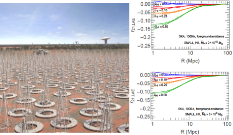
Figure 103: Left: Artist impression image of SKA low frequency array (courtesy: SKA 2018). Right: LAE-21cm cross correlation functions for the average neutral hydrogen fractions of $x_{\rm HI}=0$ (blue dot-dashed lines), $0.10$ (red long-dashed lines), $0.25$ (orange dashed lines), and $0.50$ (green short-dashed lines) that are predicted by numerical simulations (Sobacchi et al., 2016). The shades indicate the total uncertainties of theoretical models and observations including foreground effects. These calculations assume SKA1-Low 1000 hour observations for the 21cm data and the HSC survey for the LAE data (Ouchi et al., 2018). The top and bottom panels present the results of LAEs’ host halo masses of $2\times 10^{10}$ and $3\times 10^{9}$ $M_{\odot}$, respectively. This figure is reproduced by permission of the MNRAS.

Trying Other Approaches

In Sections 7.2 and 7.2, I have introduced the next-generation powerful instruments in the on-going and future programs. These next-generation instruments cover the unexplored parameter space, and are useful for resolving the issues of the open questions. However, even with no next-generation instruments, one can make a breakthrough with the present-generation instruments by a new approach. There are two observation examples in such breakthrough studies. One is the polarization observations for LABs conducted by Hayes et al. (2011b) and Prescott et al. (2011). Hayes et al. (2011b) have performed the polarization observations with VLT/FORS for a bright LAB, and detected the tangential polarization indicating the Ly$\alpha$ photon scattering in the LAB (Section LABEL:sec:lya_blob). Another example is the identifications of luminous SNe (SNe IIn) hosted by high-$z$ galaxies, $z\sim 2-4$ LBGs and LAEs (Cooke et al., 2012). Cooke et al. (2012) have investigated variables in these high-$z$ galaxies selected in the CFHT Legacy Survey data. Although it was well known that the popular bright SNe, SNe Ia, at $z\sim 2-4$ were too faint to be detected with the present data, Cooke et al. (2012) successfully found luminous SNe in the $z\sim 2-4$ galaxies. These are two good examples of making a breakthrough discovery with the existing facilities and data, if one takes new approaches. I would suggest young astronomers not to simply wait for next-generation instruments, but to try new observational approaches with existing telescopes and data.

7.3 Summary of On-Going and Future Projects

I have showcased the five major open questions related to LAEs about galaxy formation and cosmic reionization. For galaxy formation, there are four questions about i) the LAE’s distinguishing characteristics of star-formation and ISM, ii) physical origins of LABs and diffuse halos, iii) physical reasons for the large Ly$\alpha$ EW + Ly$\alpha$ escape fraction, and iv) the LAE-popIII connection. For cosmic reionization, two questions are presented: a) reionization history (late or early / sharp or extended reionization?) and b) major sources of reionization (star-forming galaxies and/or faint AGN?). These open questions are being addressed by on-going observations with the three new instruments, Subaru/HSC(+PFS), HETDEX, and VLT/MUSE. Although the observing programs of these three new instruments cover the complementary survey parameter space in redshift and depth, these programs can investigate LAEs only at $z\sim 2-7$. Beyond $z\sim 7-8$, one needs next generation large telescopes with great sensitivities, JWST, E-ELT, GMT, and TMT in the optical-IR wavelength range. Among these next generation projects, forthcoming JWST projects will probe rest-frame optical nebular lines of LAEs at $z\mathrel{\hbox{\hbox to0.0pt{\hbox{\lower 4.0pt\hbox{$\sim$}}\hss}\hbox{$>$}}}5$ for testing popIII, and conduct the unbiased search for LAEs at $z\sim 6-17$. Beyond the optical-IR wavelength range, 21cm observations with HERA and SKA will provide important results. Theoretical studies suggest that the early-phase low-frequency array of SKA1-Low and Subaru/HSC will identify a signal of spatial anti-correlation between 21 cm emission and LAEs. Although these new facilities are key for exciting discoveries, there exist examples that new observational approaches with existing facilities can also make a breakthrough. With these examples in hand, I encourage young astronomers not to simply wait for next-generation instruments, but try new observational approaches for LAE studies with the existing facilities.

8 Grand Summary for this Series of Lectures

Observations of high-$z$ LAEs and the related scientific subjects are detailed in this series of lecturers. After I explain the background of LAE discoveries, I clarify that LAEs are important objects for studying galaxy formation and cosmic reionization (Section 1). This is because LAEs are unique probes for high-$z$/low-mass (popIII-like) galaxies and the IGM Hi gas via resonance scattering and damping wing absorptions. I then overview the basic theoretical ideas of galaxy formation including structure formation, gas cooling/feedback, and the five Ly$\alpha$ emission mechanisms (Section 2). In Section 3, I summarize the physical properties of LAEs, known to date, stellar populations, luminosity functions, morphologies, ISM state, LAE-AGN connection, and hosting halos. Section LABEL:sec:galaxy_formationIII discusses the observational challenges of LAE properties; extended Ly$\alpha$ halos, Ly$\alpha$ escape fraction, and LAE-popIII connection. This series of lectures moves to cosmic reionization science in Section LABEL:sec:cosmic_reionizationI. Evolution of neutral hydrogen fraction (i.e. cosmic reionization history) is constrained by the estimates of the IGM Ly$\alpha$ absorption including the Ly$\alpha$ damping wing absorption. The combination of the Ly$\alpha$ absorption, CMB, and Hi 21 cm data provides the rough picture of reionization history. In Section LABEL:sec:cosmic_reionizationII, I explain simple analytic formulae to evaluate sources of reionization with three parameters for the ionizing photon production rate and one parameter for the IGM spatial distribution, and discuss whether star-forming galaxies can be major sources of reionization. The observational results suggest that star-forming galaxies alone can explain cosmic reionization, although the contribution of faint AGNs and the other sources are poorly understood, to date. Section LABEL:sec:ongoing_and_future_projects lists up the five open questions about LAEs, and explains three on-going projects for LAEs at $z\sim 2-7$ (Subaru/HSC+PFS, HETDEX, and VLT/MUSE) and various future optical-IR telescope projects for LAEs at $z\mathrel{\hbox{\hbox to0.0pt{\hbox{\lower 4.0pt\hbox{$\sim$}}\hss}\hbox{$>$}}}7-8$ (JWST and ground-based extremely large telescopes), together with low-frequency 21-cm observations (HERA and SKA), including some examples of science cases.

In the past two decades, I find that high-$z$ LAE studies are one of the most important driving forces for the state-of-the-art observational facilities. The importance of Ly$\alpha$ emission is undoubted, due to the fact that Ly$\alpha$ is the strongest emission for the most abundant element in the universe, namely hydrogen. Moreover, the resonance nature of Ly$\alpha$ photons allows us to probe the distribution and kinematics of neutral hydrogen in any cosmic structures of galaxies and LSSs, from the ISM to the CGM and the IGM. In the coming decade, Ly$\alpha$ observations will continue leading the field of high-$z$ observations with the on-going and future facilities. I hope that some of the readers will conduct new Ly$\alpha$ studies inspired by this series of lectures, and produce exciting results very soon.