Exponential integrators preserving first integrals or Lyapunov functions for conservative or dissipative systems

Abstract.

In this paper, combining the ideas of exponential integrators and discrete gradients, we propose and analyze a new structure-preserving exponential scheme for the conservative or dissipative system $\dot{y}=Q(My+\nabla U(y))$, where $Q$ is a $d\times d$ skew-symmetric or negative semidefinite real matrix, $M$ is a $d\times d$ symmetric real matrix, and $U:\mathbb{R}^{d}\rightarrow\mathbb{R}$ is a differentiable function. We present two properties of the new scheme. The paper is accompanied by numerical results that demonstrate the remarkable superiority of our new scheme in comparison with other structure-preserving schemes in the scientific literature.

1. Introduction

The IVP

(1) $$\dot{y(t)} =Ay(t)+f(y(t)),\quad{y(t_{0})=y^{0},}$$

arises most frequently in a variety of applications such as mechanics, molecular dynamics, quantum physics, circuit simulations and engineering, where $f:\mathbb{R}^{d}\rightarrow\mathbb{R}^{d}$ and $\cdot$ denotes the derivative operator $\frac{d}{dt}$. An algorithm for (1) is an exponential integrator if it involves the computation of matrix exponential (or related matrix functions) and integrates the linear system

$$\dot{y(t)}-Ay(t)=0$$

exactly. In general, exponential integrators permit larger stepsizes and achieve higher accuracy than non-exponential ones when (1) is a very stiff differential equation such as highly oscillatory ODEs and semi-discrete time-dependent PDEs. Therefore, numerous exponential algorithms have been proposed for first-order (see, e.g. [1, 10, 20, 22, 23, 24, 25, 26, 30]) and second-order (see e.g. [11, 12, 14, 18, 33]) ODEs. On the other hand, (1) might inherit many important geometrical/physical structures. For example, the canonical Hamiltonian system

(2) $$\dot{y(t)} =J^{-1}\nabla H(y(t)),\quad{y(t_{0})=y^{0},}$$

is a special case of (1), with

$$J=\left(\begin{array}[]{cc}O_{d_{1}\times d_{1}}&I_{d_{1}\times d_{1}}\\ -I_{d_{1}\times d_{1}}&O_{d_{1}\times d_{1}}\end{array}\right).$$

And the flow of (2) preserves the symplectic 2-form $dy\wedge Jdy$ and the function $H(y)$. In the sense of geometric integration, it is a natural idea to design numerical schemes that preserve the two structures. As far as we know, most of research papers dealing with exponential integrators up to now focus on the constructions of high-order explicit schemes and fail to be structure-preserving except for symmetric/symplectic/energy-preserving methods for first-order ODEs in [5, 7] and oscillatory second-order ODEs (see, e.g. [18, 31, 32]). To combine ideas of exponential integrators and energy-preserving methods, we address ourselves to the system:

(3) $$\dot{y}=Q(My+\nabla U(y)),\quad{y(t_{0})=y^{0},}$$

where $Q$ is a $d\times d$ real matrix, $M$ is a $d\times d$ symmetric real matrix and $U:\mathbb{R}^{d}\rightarrow\mathbb{R}$ is a differentiable function. Clearly, (3) could be considered as a special class of (1) or the generalization of (2). However, (3) concentratively exhibits some important structures which should be respected by a structure-preserving scheme. Since $M$ is symmetric, $My+\nabla U(y)$ is the gradient of the function $H(y)=\frac{1}{2}y^{\intercal}My+U(y)$. If $Q$ is skew-symmetric, then (3) is a conservative system with the first integral $H$, i.e. $H(y(t))$ is constant; If $Q$ is negative semi-definite (denoted by $Q\leq 0$), then (3) is a dissipative system with the Lyapunov function $H$, i.e. $H(y(t))$ is monotonically decreasing. In these two cases, $H$ is also called ‘energy’. It should be noted that the choice for $A$ in (1) or $M$ in (3) is not unique. General speaking, exponential integrators deal with systems having a major linear term and a comparably small nonlinear term, i.e. $||A||\gg||\frac{\partial f}{\partial y}||$. Thus, in order to take advantage of exponential integrators, the matrix $M$ in (3) should be chosen such that $||QM||\gg||QHess(U)||$, where $Hess(U)$ is the Hessian matrix of $U$. For example, highly oscillatory Hamiltonian systems can be characterized by (3) with a dominant linear part, where $M$ implicitly contain the large frequency component. Up to now, many energy-preserving or energy-decaying methods have been proposed in the case of $M=0$ (see, e.g. [3, 4, 15, 17, 19, 29]). However, these general-purpose methods are not suitable for dealing with (3) when $||QM||$ is very large. Firstly, numerical solutions generated by them are far from accurate. They are generally implicit and iterative solutions are required at each step. But the fixed-point iterations for them are not convergent unless the stepsize is tiny enough. As mentioned at the beginning, the two obstacles are hopeful of overcoming by introducing exponential integrators. In [31], the authors proposed an energy-preserving AAVF integrator (a Trigonometric method) dealing with the second-order Hamiltonian system:

$$\left\{\begin{aligned} &\ddot{q}(t)+\tilde{M}q(t)=\nabla V(q(t)),\quad\text{$\tilde{M}$ is a symmetric matrix},\\ &q(t_{0})=q_{0},\quad\dot{q}(t_{0})=\dot{q}_{0},\\ \end{aligned}\right.$$

which falls into the class of (3) by introducing $\dot{q}=p$. In this paper, we present and analyse a new exponential integrator for (3) which can preserve the first integral or the Lyapunov function.

The plan of this paper is as follows. In Section 2, we construct a general structure-preserving scheme for (3). In Section 3, we discuss two important properties of the scheme. Then we present a list of problems which can be solved by this scheme in Section 4. Numerical results including the comparison between our new scheme and other structure-preserving schemes in the literature are shown in section 5. The last Section is concerned with the conclusion.

2. Construction of the structure-preserving scheme for conservative and dissipative systems

Preliminaries 2.1.

Throughout this paper, given a holomorphic function $f$ in the neighborhood of zero ($f(0):=\lim\limits_{z\to 0}f(z)$ if  $0$ is a removable singularity ):

$$f(z)=\sum_{i=0}^{\infty}\frac{f^{(i)}(0)}{i!}z^{i},$$

and a matrix $A$, the matrix-valued function $f(A)$ is defined by :

$$f(A)=\sum_{i=0}^{\infty}\frac{f^{(i)}(0)}{i!}A^{i}.$$

$I$ and $O$ always denote identity and zero matrices of appropriate dimensions respectively. $A^{\frac{1}{2}}$ is a square root (not necessarily principal) of a symmetric matrix $A$. If $f^{(i)}(0)=0$ for odd $i$, then $f(A^{\frac{1}{2}})$ is well-defined for every symmetric $A$ (independent of the choice of $A^{\frac{1}{2}}$). Readers are referred to [21] for details about functions of matrices.

It is well known that the discrete gradient (DG) method is a popular tool for constructing energy-preserving schemes. Broadly speaking, $\overline{\nabla}H(y,\hat{y})$ is said to be a discrete gradient of function $H$ if

(4) $$\left\{\begin{aligned} &\overline{\nabla}H(y,\hat{y})^{\intercal}(y-\hat{y})=H(y)-H(\hat{y}),\\ &\overline{\nabla}H(y,y)=\nabla H(y).\\ \end{aligned}\right.$$

Accordingly,

(5) $$y^{1}=y^{0}+hJ^{-1}\overline{\nabla}H(y^{1},y^{0})$$

is called a DG method for the system (2). Multiplying $\overline{\nabla}H(y^{1},y^{0})^{\intercal}$ on both sides of (5) and using the first identity of (4), we obtain $H(y^{1})=H(y^{0})$, i.e. the scheme (5) is energy-preserving. For more details on the DG method, readers are referred to [15, 28].

On the other hand, most of exponential integrators can be derived from the variation-of-constants formula for the problem (3):

(6) $$y(t_{0}+h)=\exp(hQM)y(t_{0})+h\int_{0}^{1}\exp((1-\xi)hQM)Q\nabla U(y(t_{0}+\xi h))d\xi.$$

Replacing $\nabla U(y(t_{0}+\xi h))$ with the discrete gradient $\overline{\nabla}U(y^{1},y^{0})$, the integral in (6) can be approximated by :

$$\int_{0}^{1}\exp((1-\xi)hQM)Q\nabla U(y(t_{0}+\xi h))d\xi$$

$$\approx(\int_{0}^{1}\exp((1-\xi)hQM)d\xi)Q\overline{\nabla}U(y^{1},y^{0})=\varphi(hQM)Q\overline{\nabla}U(y^{1},y^{0}),$$

where the scalar function is given by

$$\varphi(z)=(\exp(z)-1)/z.$$

Then we obtain the new scheme:

(7) $$y^{1}=\exp(V)y^{0}+h\varphi(V)Q\overline{\nabla}U(y^{1},y^{0}),$$

where $V=hQM$ and $y^{1}\approx y(t_{0}+h)$.

Due to the energy-preserving property of the DG method, we are hopeful of preserving the first integral by (7) when $Q$ is skew. For convenience, we denote $\overline{\nabla}U(y^{1},y^{0})$ by $\overline{\nabla}U$ sometimes. To begin with, we give the following preliminary lemma.

Lemma 2.2.

For any symmetric matrix $M$ and scalar $h\geq 0$, the matrix

$$B=\exp(hQM)^{\intercal}M\exp(hQM)-M$$

satisfies:

$$B=\left\{\begin{aligned} &=0,\quad\text{if $Q$ is skew-symmetric,}\\ &\leq 0,\quad\text{if $Q\leq 0$.}\end{aligned}\right.$$

Proof.

Consider the linear ODE:

(8) $$\dot{y}(t)=QMy(t).$$

When $Q$ is skew, (8) is a conservative equation with the first integral $\frac{1}{2}y^{\intercal}My$, and its exact solution starting from the initial value $y(0)=y^{0}$ is $y(t)=\exp(tQM)y^{0}$. From $\frac{1}{2}y(h)^{\intercal}My(h)=\frac{1}{2}y^{0\intercal}My^{0}$, we have

$$\ \frac{1}{2}y^{0\intercal}\exp(hQM)^{\intercal}M\exp(hQM)y^{0}=\frac{1}{2}y^{0\intercal}My^{0}$$

for any vector $y^{0}$. Therefore, $B=\exp(hQM)^{\intercal}M\exp(hQM)-M$ is skew-symmetric. Since it is also symmetric, $B=0$. The case that $Q\leq 0$ can be proved in a similar way. ∎

Theorem 2.3.

If $Q$ is skew-symmetric, then the scheme (7) preserves the first integral $H$ in (3) exactly :

$$H(y^{0})=H(y^{1}),$$

where $H(y)=\frac{1}{2}y^{\intercal}My+U(y)$.

Proof.

Here we firstly assume that the matrix $M$ is not singular. We next calculate $\frac{1}{2}y^{1\intercal}My^{1}$. Let $M^{-1}\overline{\nabla}U=\widetilde{\nabla}U$. Replacing $y^{1}$ by $\exp(V)y^{0}+h\varphi(V)Q\overline{\nabla}U(y^{1},y^{0})$ leads to

(9) $$\frac{1}{2}y^{1\intercal}My^{1}$$

$$=\frac{1}{2}(y^{0\intercal}\exp(V)^{\intercal}+h\overline{\nabla}U^{\intercal}Q^{\intercal}\varphi(V)^{\intercal})M(\exp(V)y^{0}+h\varphi(V)Q\overline{\nabla}U)$$

$$=\frac{1}{2}y^{0\intercal}\exp(V)^{\intercal}M\exp(V)y^{0}+hy^{0\intercal}\exp(V)^{\intercal}M\varphi(V)Q\overline{\nabla}U+\frac{h^{2}}{2}\overline{\nabla}U^{\intercal}Q^{\intercal}\varphi(V)^{\intercal}M\varphi(V)Q\overline{\nabla}U$$

$$=\frac{1}{2}y^{0\intercal}\exp(V)^{\intercal}M\exp(V)y^{0}+y^{0\intercal}\exp(V)^{\intercal}M\varphi(V)V\widetilde{\nabla}U+\frac{1}{2}\widetilde{\nabla}U^{\intercal}V^{\intercal}\varphi(V)^{\intercal}M\varphi(V)V\widetilde{\nabla}U\quad(\text{using }V=hQM)$$

$$=\frac{1}{2}y^{0\intercal}\exp(V)^{\intercal}M\exp(V)y^{0}+y^{0\intercal}\exp(V)^{\intercal}M(\exp(V)-I)\widetilde{\nabla}U$$

$$+\frac{1}{2}\widetilde{\nabla}U^{\intercal}(\exp(V)^{\intercal}-I)M(\exp(V)-I)\widetilde{\nabla}U\quad(\text{using }\varphi(V)V=\exp(V)-I)$$

$$=\frac{1}{2}y^{0\intercal}\exp(V)^{\intercal}M\exp(V)y^{0}+y^{0\intercal}(\exp(V)^{\intercal}M\exp(V)-\exp(V)^{\intercal}M)\widetilde{\nabla}U$$

$$+\frac{1}{2}\widetilde{\nabla}U^{\intercal}(\exp(V)^{\intercal}M\exp(V)-\exp(V)^{\intercal}M-M\exp(V)+M)\widetilde{\nabla}U.$$

On the other hand, it follows from the property of the discrete gradient (4) that

(10) $$U(y^{1})-U(y^{0})$$

$$=(y^{1\intercal}-y^{0\intercal})\overline{\nabla}U(y^{1},y^{0})$$

$$=y^{0\intercal}(\exp(V)^{\intercal}-I)\overline{\nabla}U+h\overline{\nabla}U^{\intercal}Q^{\intercal}\varphi(V)^{\intercal}\overline{\nabla}U$$

$$=y^{0\intercal}(\exp(V)^{\intercal}M-M)\widetilde{\nabla}U+\widetilde{\nabla}U^{\intercal}V^{\intercal}\varphi(V)^{\intercal}M\widetilde{\nabla}U$$

$$=y^{0\intercal}(\exp(V)^{\intercal}M-M)\widetilde{\nabla}U+\widetilde{\nabla}U^{\intercal}(\exp(V)^{\intercal}M-M)\widetilde{\nabla}U.$$

Combining (9), (10) and collecting terms by types ‘$y^{0\intercal}*y^{0}$’, ‘$y^{0\intercal}*\widetilde{\nabla}U$’, ‘$\widetilde{\nabla}U^{\intercal}*\widetilde{\nabla}U$’ leads to

(11) $$H(y^{1})-H(y^{0})$$

$$=\frac{1}{2}y^{1\intercal}My^{1}-\frac{1}{2}y^{0\intercal}My^{0}+U(y^{1})-U(y^{0})$$

$$=\frac{1}{2}y^{0\intercal}(\exp(V)^{\intercal}M\exp(V)-M)y^{0}+y^{0\intercal}(\exp(V)^{\intercal}M\exp(V)-M)\widetilde{\nabla}U$$

$$+\frac{1}{2}\widetilde{\nabla}U^{\intercal}(\exp(V)^{\intercal}M\exp(V)-M)\widetilde{\nabla}U+\frac{1}{2}\widetilde{\nabla}U^{\intercal}(\exp(V)^{\intercal}M-M\exp(V))\widetilde{\nabla}U$$

$$=\frac{1}{2}(y^{0}+\widetilde{\nabla}U)^{\intercal}B(y^{0}+\widetilde{\nabla}U)+\frac{1}{2}\widetilde{\nabla}U^{\intercal}C\widetilde{\nabla}U=0,$$

where $B=\exp(V)^{\intercal}M\exp(V)-M$ and $C=\exp(V)^{\intercal}M-M\exp(V)$. The last step is from the skew-symmetry of the matrix $B$ (according to Lemma 2.2) and $C$.

If $M$ is singular, it is easy to find a series of symmetric and nonsingular matrices $\{M_{\varepsilon}\}$ which converge to $M$ when $\varepsilon\to 0.$ Thus, according to the result stated above, it still holds that

(12) $$H_{\varepsilon}(y_{\varepsilon}^{1})=H_{\varepsilon}(y^{0})$$

for all $\varepsilon,$ where $H_{\varepsilon}(y)=\frac{1}{2}y^{\intercal}M_{\varepsilon}y+U(y)$ is the first integral of the perturbed problem

$$\dot{y}=Q(M_{\varepsilon}y+\nabla U(y)),\quad{y(t_{0})=y^{0}},$$

and

$$y_{\varepsilon}^{1}=\exp(V_{\varepsilon})y^{0}+h\varphi(V_{\varepsilon})Q\overline{\nabla}U(y_{\varepsilon}^{1},y^{0}),\quad V_{\varepsilon}=hQM_{\varepsilon}.$$

Therefore, when $\varepsilon\to 0$, $y^{1}_{\varepsilon}\to y^{1}$ and (12) leads to

$$H(y^{1})=H(y^{0}).$$

This completes the proof. ∎

∎

Moreover, the scheme (7) can also model the decay of the Lyapunov function once $Q\leq 0$ in (3). The next theorem shows this point.

Theorem 2.4.

If $Q$ is negative semi-definite (not necessary to be symmetric), then the scheme (7) preserves the Lyapunov function $H$ in (3):

$$H(y^{1})\leq H(y^{0}),$$

where $H(y)=\frac{1}{2}y^{\intercal}My+U(y)$.

Proof.

If $M$ is nonsingular, the equation in (11)

$$H(y^{1})-H(y^{0})=\frac{1}{2}(y^{0}+\widetilde{\nabla}U)^{\intercal}B(y^{0}+\widetilde{\nabla}U)$$

still holds, since the derivation does not depend on the skew-symmetry of $Q$. By Lemma 2.2, $B$ is negative semi-definite. Thus $H(y^{1})\leq H(y^{0}).$ In the case that $M$ is singular, this theorem can be easily proved by replacing the equalities

$$H_{\varepsilon}(y_{\varepsilon}^{1})=H_{\varepsilon}(y^{0}),\quad H(y^{1})=H(y^{0})$$

in the proof of Theorem 2.3 with the inequalities

$$H_{\varepsilon}(y_{\varepsilon}^{1})\leq H_{\varepsilon}(y^{0}),\quad H(y^{1})\leq H(y^{0}).$$

∎

We here skip the details.∎

In this paper, we choose the average vector field (AVF) as the discrete gradient in (7). The corresponding scheme for (3) now is

(13) $$y^{1} =\exp(V)y^{0}+h\varphi(V)Q\int_{0}^{1}\nabla U((1-\tau)y^{0}+\tau y^{1})d\tau,$$

where $V=hQM$ and $y^{1}\approx y(t_{0}+h)$. (13) is called an exponential AVF integrator and denoted by EAVF.

3. Properties of EAVF

In this section, we present two properties of EAVF as follows.

Theorem 3.1.

The EAVF integrator (13) is symmetric.

Proof.

Exchanging $y^{0}\leftrightarrow y^{1}$ and replacing $h$ by $-h$ in (13), we obtain

(14) $$y^{0}=\exp(-V)y^{1}-h\varphi(-V)Q\int_{0}^{1}\nabla U((1-\tau)y^{1}+\tau y^{0})d\tau.$$

Rewrite (14) as:

(15) $$y^{1}=\exp(V)y^{0}+h\exp(V)\varphi(-V)Q\int_{0}^{1}\nabla U((1-\tau)y^{0}+\tau y^{1})d\tau.$$

Since $\exp(V)\varphi(-V)=\varphi(V)$, (15) is the same as (13) exactly, which means that EAVF is symmetric. ∎

∎

It should be noted that the scheme (13) is implicit in general, and thus iteration solutions are required. Next, we discuss the convergence of the fixed-point iteration for the EAVF integrator.

Theorem 3.2.

Suppose that $||\varphi(V)||_{2}\leq C$, $\nabla U(u)$ satisfies the Lipschitz condition, i. e. there exists a constant L such that

$$||\nabla U(v)-\nabla U(w)||_{2}\leq L||v-w||_{2}.$$

If

(16) $$0<h\leq\hat{h}<\frac{2}{CL||Q||_{2}}$$

then the iteration

$$\Psi:z\mapsto\exp(V)y^{n}+h\varphi(V)Q\int_{0}^{1}\nabla U((1-\tau)y^{n}+\tau z)d\tau$$

for the EAVF integrator (13) is convergent.

Proof.

Since

$$||\Psi(z_{1})-\Psi(z_{2})||_{2}$$

$$=||h\varphi(V)Q\int_{0}^{1}(\nabla U((1-\tau)y^{n}+\tau z_{1})-\nabla U((1-\tau)y^{n}+\tau z_{2}))d\tau||_{2}$$

$$\leq\frac{h}{2}CL||Q||_{2}||z_{1}-z_{2}||_{2}\leq\frac{\hat{h}}{2}CL||Q||_{2}||z_{1}-z_{2}||_{2}=\rho||z_{1}-z_{2}||_{2},$$

where

$$\rho=\frac{\hat{h}}{2}CL||Q||_{2}<1,$$

the iteration $\Psi$ converges by (16) and Contraction Mapping Theorem. ∎

∎

Remark 3.3.

We note two special and important cases in practical applications. If $QM$ is skew-symmetric or symmetric negative semi-definite, then the spectrum of $V$ lies in the left half-plane. Since $QM$ is unitarily diagonalizable and $|\varphi(z)|\leq 1$ for any $z$ satisfying $real(z)\leq 0$, we have $||\varphi(V)||_{2}\leq 1$.

In many cases, the matrix $M$ has extremely large norm (e.g., $M$ incorporates high frequency components in oscillatory problems or $M$ is the differential matrix in semi-discrete PDEs), thus, Theorem 3.2 ensures the possibility of choosing relatively large stepsize regardless of $M$.

In practice, the integral in (13) usually cannot be easily calculated. Therefore, we can evaluate it using the $s$-point Gauss-Legendre (GL$s$) formula $(b_{i},c_{i})_{i=1}^{s}$:

$$\int_{0}^{1}\nabla U((1-\tau)y^{0}+\tau y^{1})d\tau\approx\sum_{i=1}^{s}b_{i}\nabla U((1-c_{i})y^{0}+c_{i}y^{1})).$$

The corresponding scheme is denoted by EAVFGL$s$. Since the $s$-point GL quadrature formula is symmetric, EAVFGL$s$ is also symmetric. According to $\sum_{i=1}^{s}b_{i}c_{i}=1/2$, the corresponding iteration for EAVFGL$s$ is convergent provided (16) holds.

4. Problems suitable for the EAVF

4.1. Highly oscillatory nonseparable Hamiltonian system

Consider the Hamiltonian

$$H(p,q)=\frac{1}{2}p_{1}^{\intercal}M_{1}^{-1}p_{1}+\frac{1}{2\varepsilon^{2}}q_{1}^{\intercal}A_{1}q_{1}+S(p,q),$$

where

$$p=\left(\begin{array}[]{c}p_{0}\\ p_{1}\end{array}\right),\quad q=\left(\begin{array}[]{c}q_{0}\\ q_{1}\end{array}\right)$$

are both $d$-length vectors, $M_{1},A_{1}$ are symmetric positive definite matrices, and $0<\varepsilon\ll 1$. This Hamiltonian governs oscillatory mechanical systems in 2 or 3 space dimensions such as the stiff spring pendulum and the dynamics of the multi-atomic molecule (see, e.g. [8, 9]). After an appropriate canonical transformation (see, e.g. [18]), this Hamiltonian becomes:

(17) $$H(p,q)=\frac{1}{2}\sum_{j=1}^{l}(p_{1,j}^{2}+\frac{\lambda_{j}^{2}}{\varepsilon^{2}}q_{1,j}^{2})+S(p,q),$$

where $p_{1}=(p_{1,1},\ldots,p_{1,l})^{\intercal},q_{1}=(q_{1,1},\ldots,q_{1,l})^{\intercal}$. The corresponding equation is given by

(18) $$\left\{\begin{aligned} &\dot{p_{0}}=-\nabla_{q_{0}}S(p,q),\\ &\dot{p_{1}}=-\omega^{2\intercal}q_{1}-\nabla_{q_{1}}S(p,q),\\ &\dot{q_{0}}=p_{0}+(\nabla_{p_{0}}S(p,q)-p_{0}),\\ &\dot{q_{1}}=p_{1}+\nabla_{p_{1}}S(p,q),\\ \end{aligned}\right.$$

where $\omega=(\omega_{1},\ldots,\omega_{l})^{\intercal},\omega_{j}=\lambda_{j}/\varepsilon$ for $j=1,\ldots,l$. (LABEL:NSP) is of the form (3) :

$$y=\left(\begin{array}[]{c}p\\ q\end{array}\right),\quad Q=\left(\begin{array}[]{cc}O&-I_{d\times d}\\ I_{d\times d}&O\end{array}\right),\quad M=\left(\begin{array}[]{cc}I_{d\times d}&O\\ O&\Omega_{d\times d}\end{array}\right),$$

and

$$U(p,q)=S(p,q)-\frac{1}{2}p_{0}^{\intercal}p_{0},\quad\Omega=diag(0,\ldots,0,\omega_{1}^{2},\ldots,\omega_{l}^{2}).$$

Since $q_{11},\ldots,q_{1l}$ and $p_{11},\ldots,p_{1l}$ are fast variables, it is favorable to integrate the linear part of them exactly by the scheme (13). Note that

$$\varphi(V)=\left(\begin{array}[]{cc}sinc(h\Omega^{\frac{1}{2}})&h^{-1}g_{2}(h\Omega^{\frac{1}{2}})\\ hg_{1}(h\Omega^{\frac{1}{2}})&sinc(h\Omega^{\frac{1}{2}})\end{array}\right),$$

where $sinc(z)=\sin(z)/z,g_{1}(z)=(1-\cos(z))/z^{2},g_{2}(z)=\cos(z)-1$. Unfortunately, the block $h^{-1}g_{2}(h\Omega^{\frac{1}{2}})$ is not uniformly bounded. In the first experiment, the iteration still works well, perhaps due to the small Lipshitz constant of $\nabla S$.

4.2. Second-order (damped) highly oscillatory system

Consider

(19) $$\ddot{q}-N\dot{q}+\Omega q=-\nabla U_{1}(q),$$

where $q$ is a $d$-length vector variable, $U_{1}:\mathbb{R}^{d}\to\mathbb{R}$ is a differential function, $N$ is a symmetric negative semi-definite matrix, $\Omega$ is a symmetric positive semi-definite matrix, $||\Omega||$ or $||N||\gg 1$. (19) stands for highly oscillatory problems such as the dissipative molecular dynamics, the (damped) Duffing and semi-discrete nonlinear wave equations. By introducing $p=\dot{q},$ we write (19) as a first-order system of ODEs :

(20) $$\left(\begin{array}[]{c}\dot{q}\\ \dot{p}\end{array}\right)=\left(\begin{array}[]{cc}O&I\\ -\Omega&N\end{array}\right)\left(\begin{array}[]{c}q\\ p\end{array}\right)+\left(\begin{array}[]{c}0\\ -\nabla U_{1}(q)\end{array}\right),$$

which falls into the class (3), where

$$y=\left(\begin{array}[]{c}q\\ p\end{array}\right),Q=\left(\begin{array}[]{cc}O&I\\ -I&N\end{array}\right),M=\left(\begin{array}[]{cc}\Omega&O\\ O&I\end{array}\right),U(y)=\left(\begin{array}[]{c}U_{1}(q)\\ O\end{array}\right).$$

Clearly, $Q\leq 0$ and (20) is a dissipative system with the Lyapunov function $H=\frac{1}{2}p^{\intercal}p+\frac{1}{2}q^{\intercal}\Omega q+U_{1}(q)$. In the particular case $N=0,$ (20) becomes a conservative Hamiltonian system. Let

$$A=QM=\left(\begin{array}[]{cc}O&I\\ -\Omega&N\end{array}\right).$$

Applying the EAVF integrator (13) to the equation (20) yields the scheme:

(21) $$\left\{\begin{aligned} &q^{1}=\exp_{11}q^{0}+\exp_{12}p^{0}-h\varphi_{12}\int_{0}^{1}\nabla U_{1}((1-\tau)q^{0}+\tau q^{1})d\tau,\\ &p^{1}=\exp_{21}q^{0}+\exp_{22}p^{0}-h\varphi_{22}\int_{0}^{1}\nabla U_{1}((1-\tau)q^{0}+\tau q^{1})d\tau,\\ \end{aligned}\right.$$

where $\exp(hA)$ and $\varphi(hA)$ are partitioned into

$$\left(\begin{array}[]{cc}\exp_{11}&\exp_{12}\\ \exp_{21}&\exp_{22}\end{array}\right)\text{ and }\left(\begin{array}[]{cc}\varphi_{11}&\varphi_{12}\\ \varphi_{21}&\varphi_{22}\end{array}\right),$$

respectively.

It should be noted that only the first equation in the scheme (21) need to be solved by iterations. From the proof procedure of Theorem 3.2, one can find that the convergence of the fixed-point iteration for (21) is irrelevant to $||A||$ provided $\varphi_{12}$ is uniformly bounded.

Theorem 4.1.

Assume that $\Omega$ commutes with $N$, $||\nabla U_{1}(v)-\nabla U_{1}(w)||_{2}\leq L||v-w||_{2}$, then the iteration

$$\Phi:z\mapsto\exp_{11}q^{0}+\exp_{12}p^{0}-h\varphi_{12}\int_{0}^{1}\nabla U_{1}((1-\tau)q^{0}+\tau z)d\tau$$

for the scheme (21) is convergent provided

$$0<h\leq\hat{h}<\frac{2}{L^{\frac{1}{2}}}.$$

Proof.

The crucial point here is to find a uniform upper bound of $||\varphi_{12}||$. Since $\Omega$ commutes with $N$, they can be simultaneously diagonalized:

$$\Omega=F^{\intercal}\Lambda F,\quad N=F^{\intercal}\Sigma F,$$

where $F$ is an orthogonal matrix, $\Lambda=diag(\lambda_{1},\ldots,\lambda_{d}),\Sigma=diag(\sigma_{1},\ldots,\sigma_{d})$ and $\lambda_{i}\geq 0,\sigma_{i}\leq 0$ for $i=1,2,\ldots,d$. It now follows from

$$A=\left(\begin{array}[]{cc}F^{\intercal}&O\\ O&F^{\intercal}\end{array}\right)\left(\begin{array}[]{cc}O&I\\ -\Lambda&\Sigma\end{array}\right)\left(\begin{array}[]{cc}F&O\\ O&F\end{array}\right)$$

that

$$\exp(hA)=\left(\begin{array}[]{cc}F^{\intercal}&O\\ O&F^{\intercal}\end{array}\right)\exp\left\{\left(\begin{array}[]{cc}O&hI\\ -h\Lambda&h\Sigma\end{array}\right)\right\}\left(\begin{array}[]{cc}F&O\\ O&F\end{array}\right).$$

To show that $\exp_{12}$ and $\varphi_{12}$ depends on $h$, we denote them by $\exp_{12}^{h}$ and $\varphi_{12}^{h}$, respectively. After some calculations, we have

$$\exp_{12}^{h}=F^{\intercal}\frac{2\sinh(h(\Sigma^{2}-4\Lambda)^{\frac{1}{2}}/2)}{(\Sigma^{2}-4\Lambda)^{\frac{1}{2}}}\exp\left(\frac{h\Sigma}{2}\right)F.$$

Then we have

(22) $$||\exp_{12}^{h}||_{2}=||\frac{2\sinh(h(\Sigma^{2}-4\Lambda)^{\frac{1}{2}}/2)}{(\Sigma^{2}-4\Lambda)^{\frac{1}{2}}}\exp\left(\frac{h\Sigma}{2}\right)||_{2}=h\max_{i}|\frac{\sinh((h^{2}\sigma_{i}^{2}/4-\lambda_{i})^{\frac{1}{2}})}{(h^{2}\sigma_{i}^{2}/4-\lambda_{i})^{\frac{1}{2}}}\exp\left(\frac{h\sigma_{i}}{2}\right)|.$$

In order to estimate $||\exp_{12}^{h}||_{2}$, the bound of the function

$$g(\lambda,\sigma)=\frac{\sinh((\sigma^{2}-4\lambda)^{\frac{1}{2}})}{(\sigma^{2}-4\lambda)^{\frac{1}{2}}}\exp\left(\sigma\right),$$

should be considered for $\sigma\leq 0,\lambda\geq 0$. If $\sigma^{2}-4\lambda<0$, we set $(\sigma^{2}-4\lambda)^{\frac{1}{2}}=ia,$ where $i$ is the imaginary unit and $a$ is a real number. Then we have

$$|g|=|\frac{\sin(a)}{a}\exp\left(\sigma\right)|\leq|\frac{\sin(a)}{a}|\leq 1.$$

If $\sigma^{2}-4\lambda\geq 0$, then $a=(\sigma^{2}-4\lambda)^{\frac{1}{2}}\leq-\sigma$,

$$|g|=|\frac{\sinh(a)}{a}\exp\left(\sigma\right)|\leq|\frac{\sinh(a)}{a}\exp(-a)|=|\frac{1-\exp(-2a)}{2a}|\leq 1.$$

Thus

(23) $$|g(\lambda,\sigma)|\leq 1\quad\text{for }\sigma\leq 0,\lambda\geq 0.$$

It follows from (22) and (23) that

(24) $$||\exp_{12}^{h}||_{2}=h\max_{i}|g(\frac{h\sigma_{i}}{2},\lambda_{i})|\leq h.$$

Therefore, using $\varphi(hA)=\int_{0}^{1}\exp((1-\xi)hA)d\xi$ and (24), we obtain

$$||\varphi_{12}^{h}||_{2}=||\int_{0}^{1}\exp_{12}^{(1-\xi)h}d\xi||_{2}\leq\int_{0}^{1}||\exp_{12}^{(1-\xi)h}||_{2}d\xi\leq\int_{0}^{1}(1-\xi)hd\xi=\frac{1}{2}h.$$

Since the rest of the proof is very similar to that of Theorem 3.2, we omit it here. ∎

∎

It can be observed that in the particular case that $N=0$, the scheme (21) reduces to the AAVF integrator in [31].

4.3. Semi-discrete conservative and dissipative PDEs

Many time-dependent PDEs are of the form :

(25) $$\partial_{t}y(x,t)=\mathcal{Q}\frac{\delta\mathcal{H}}{\delta y},$$

where $y(\cdot,t)\in X$ for every $t\geq 0$, $X$ is a Hilbert space such as $\mathbf{L}^{2}(\Omega),\mathbf{L}^{2}(\Omega)\times\mathbf{L}^{2}(\Omega),\ldots$, $\Omega$ is a domain in $\mathbb{R}^{d}$, and $\mathcal{Q}$ is a linear operator on $X$. $\mathcal{H}[y]=\int_{\Omega}H(y,\partial_{\alpha}y)dx$ ($H$ is smooth, $x=(x_{1},\ldots,x_{d}),dx=dx_{1}\ldots dx_{d}$ and $\partial_{\alpha}y$ denotes the partial derivatives of $y$ with respect to spatial variables $x_{i},1\leq i\leq d$). Under suitable boundary condition (BC), the variational derivative $\frac{\delta\mathcal{H}}{\delta y}$ is defined by :

$$\langle\frac{\delta\mathcal{H}}{\delta y},z\rangle=\frac{d}{d\varepsilon}|_{\varepsilon=0}\mathcal{H}[y+\varepsilon z]$$

for any smooth $z\in X$ satisfying the same BC, where $\langle\cdot,\cdot\rangle$ is the inner product of $X$. If $\mathcal{Q}$ is a skew or negative semi-definite operator with respect to $\langle\cdot,\cdot\rangle$, then the equation (25) is conservative (e.g., the nonlinear wave, nonlinear Schrödinger, Korteweg–de Vries and Maxwell equations) or dissipative (e.g., the Allen–Cahn, Cahn–Hilliard, Ginzburg–Landau and heat equations), i.e., $\mathcal{H}[y]$ is constant or monotonically decreasing (see, e.g. [6, 13]). In general, after the spatial discretization, (25) becomes a conservative or dissipative system of ODEs in the form (3). Here we exemplify conservative ones by the nonlinear Schrödinger equation:

(26) $$iy_{t}+y_{xx}+V^{{}^{\prime}}(|y|^{2})y=0$$

under the periodic BC $y(0,t)=y(L,t)$, where $y=p+iq$ is a complex-valued function, $p,q$ are both real, $i$ is the imaginary unit. The equation (26) is of the form (25) :

(27) $$\partial_{t}\left(\begin{array}[]{c}p\\ q\end{array}\right)=\left(\begin{array}[]{cc}0&-1\\ 1&0\end{array}\right)\left(\begin{array}[]{c}p_{xx}+V^{{}^{\prime}}(p^{2}+q^{2})p\\ q_{xx}+V^{{}^{\prime}}(p^{2}+q^{2})q\end{array}\right),$$

where $X=\mathbf{L}^{2}([0,L])\times\mathbf{L}^{2}([0,L]),\mathcal{H}[y]=\frac{1}{2}\int_{0}^{L}(V(p^{2}+q^{2})-p_{x}^{2}-q_{x}^{2})dx$. Assume that the spatial domain is equally partitioned into $N$ intervals: $0=x_{0}<x_{1}<\ldots<x_{N}=L$. Discretizing the spatial derivatives of (27) by the central difference arrives at

(28) $$\left(\begin{array}[]{c}\dot{\tilde{p}}\\ \dot{\tilde{q}}\end{array}\right)=\left(\begin{array}[]{cc}O&-I\\ I&O\end{array}\right)\left(\begin{array}[]{c}D\tilde{p}+V^{{}^{\prime}}(\tilde{p}^{2}+\tilde{q}^{2})\tilde{p}\\ D\tilde{q}+V^{{}^{\prime}}(\tilde{p}^{2}+\tilde{q}^{2})\tilde{q}\end{array}\right),$$

where

$$D=\left(\begin{array}[]{ccccc}-2&1&&&\\ 1&-2&1&&\\ &\ddots&\ddots&\ddots&\\ &&1&-2&1\\ &&&1&-2\end{array}\right),$$

is an $N\times N$ symmetric differential matrix, $\tilde{p}=(p_{0},\ldots,p_{N-1})^{\intercal},\tilde{q}=(q_{0},\ldots,q_{N-1})^{\intercal},p_{i}(t)\approx p(x_{i},t)$ and $q_{i}(t)\approx q(x_{i},t)$ for $i=0,\ldots,N-1$.

An example of dissipative PDEs is the Allen-Cahn equation:

(29) $$y_{t}=dy_{xx}+y-y^{3},\quad d\geq 0$$

under the the Neumann BC $y_{x}(0,t)=y_{x}(L,t)$. $X=\mathbf{L}^{2}([0,L]),\mathcal{Q}=-1,\mathcal{H}[y]=\int(\frac{1}{2}dy_{x}^{2}-\frac{1}{2}y^{2}+\frac{1}{4}y^{4})dx$. The spatial grids are chosen in the same way as NLS. Discretizing the spatial derivative by the central difference, we obtain

(30) $$\dot{\tilde{y}}=d\hat{D}\tilde{y}+\tilde{y}-\tilde{y}^{3},$$

where

$$\hat{D}=\left(\begin{array}[]{ccccc}-1&1&&&\\ 1&-2&1&&\\ &\ddots&\ddots&\ddots&\\ &&1&-2&1\\ &&&1&-1\end{array}\right),$$

is the $(N-1)\times(N-1)$ symmetric differential matrix, $\tilde{y}=(y_{1},\ldots,y_{N-1})^{\intercal},y_{i}(t)\approx y(x_{i},t)$.

Both the semi-discrete NLS equation (28) and AC equation (30) are of the form (3). For the NLS and the AC equations, we have

$$Q=\left(\begin{array}[]{cc}O&-I\\ I&O\end{array}\right),\quad M=\left(\begin{array}[]{cc}D&O\\ O&D\end{array}\right),\quad U=\frac{1}{2}\sum_{i=0}^{N-1}V(p_{i}^{2}+q_{i}^{2}),$$

and

$$Q=-I,\quad M=-d\hat{D},\quad U=\sum_{i=1}^{N-1}(-\frac{1}{2}y_{i}^{2}+\frac{1}{4}y_{i}^{4}).$$

respectively. Therefore, the scheme (13) can be applied to solve them. Since the matrix $QM$ is skew or symmetric negative semi-definite in these two cases, according to the Remark 3.3, the convergence of fixed-point iterations for them is independent of the differential matrix.

5. Numerical experiments

In this section, we compare the EAVF method (13) with the well-known implicit midpoint method which is denoted by MID:

(31) $$y^{1}=y^{0}+hQ\nabla\widetilde{U}(\frac{y^{0}+y^{1}}{2}),$$

and the traditional AVF method for the equation (3) is given by

(32) $$y^{1}=y^{0}+hQ\int_{0}^{1}\nabla\widetilde{U}((1-\tau)y^{0}+\tau y^{1})d\tau,$$

where $\widetilde{U}(y)=U(y)+\frac{1}{2}y^{\intercal}My$. The authors in [28] showed that (32) preserves the first integral or the Lyapunov function $\widetilde{U}$. Our comparison also includes another energy-preserving method of order four for (3) :

(33) $$\left\{\begin{aligned} &y^{\frac{1}{2}}=y^{0}+hQ\int_{0}^{1}(\frac{5}{4}-\frac{3}{2}\tau)\nabla\widetilde{U}(y_{\tau})d\tau,\\ &y^{1}=y^{0}+hQ\int_{0}^{1}\nabla\widetilde{U}(y_{\tau})d\tau,\\ \end{aligned}\right.$$

where

$$y_{\tau}=(2\tau-1)(\tau-1)y^{0}-4\tau(\tau-1)y^{\frac{1}{2}}+(2\tau-1)\tau y^{1}.$$

This method is denoted by CRK since it can be written as a continuous Runge–Kutta method. For details, readers are referred to [17].

Throughout the experiment, the ‘reference solution’ is computed by high-order methods with a sufficiently small stepsize. We always start to calculate from $t_{0}=0$. $y^{n}\approx y(t_{n})$ is obtained by the time-stepping way $y^{0}\rightarrow y^{1}\rightarrow\cdots\rightarrow y^{n}\rightarrow\cdots$ for $n=1,2,\ldots$ and $t_{n}=nh$. The error tolerance for iteration solutions of the four methods is set as $10^{-14}$. The maximum global error (GE) over the total time interval is defined by:

$$GE=\max_{n\geq 0}||y^{n}-y(t_{n})||_{\infty}.$$

The maximum global error of $H$ ($EH$) on the interval is:

$$EH=\max_{n\geq 0}|H^{n}-H(y(t_{n}))|.$$

In our numerical experiments, the computational cost of each method is measured by the number of function evaluations (FE).

Problem 5.1.

The motion of a triatomic molecule can be modeled by a Hamiltonian system with the Hamiltonian of the form (17) (see, e.g. [8]):

(34) $$H(p,q)=S(p,q)+\frac{1}{2}(p_{1,1}^{2}+p_{1,2}^{2}+p_{1,3}^{2})+\frac{\omega^{2}}{2}(q_{1,1}^{2}+q_{1,2}^{2}+q_{1,3}^{2}),$$

where

$$S(p,q)=\frac{1}{2}p_{0}^{2}+\frac{1}{4}(q_{0}-q_{1,3})^{2}-\frac{1}{4}\frac{2q_{1,2}+q_{1,2}^{2}}{(1+q_{1,2})^{2}}(p_{0}-p_{1,3})^{2}-\frac{1}{4}\frac{2q_{1,1}+q_{1,1}^{2}}{(1+q_{1,1})^{2}}(p_{0}+p_{1,3})^{2}.$$

The initial values are given by :

$$\left\{\begin{aligned} &p_{0}(0)=p_{1,1}(0)=p_{1,2}(0)=p_{1,3}(0)=1,\\ &q_{0}(0)=0.4,q_{1,1}(0)=q_{1,2}(0)=\frac{1}{\omega},q_{1,3}=\frac{1}{2^{\frac{1}{2}}\omega}.\\ \end{aligned}\right.$$

Setting $h=1/2^{i},i=6,\ldots,10,\omega=50$ and $h=1/100\times 1/2^{i},i=0,\ldots,4,\omega=100$, we integrate the problem (LABEL:NSP) with the Hamiltonian (34) over the interval $[0,50]$. Since the nonlinear term $\nabla S(p,q)$ is complicated to be integrated, we evaluate the integrals in EAVF, AVF and CRK by the $3$-point Gauss–Legendre (GL) quadrature formula $(b_{i},c_{i})_{i=1}^{3}$:

$$b_{1}=\frac{5}{18},b_{2}=\frac{4}{9},b_{3}=\frac{5}{18};\quad c_{1}=\frac{1}{2}-\frac{15^{\frac{1}{2}}}{10},c_{2}=\frac{1}{2},c_{3}=\frac{1}{2}+\frac{15^{\frac{1}{2}}}{10}.$$

Corresponding schemes are denoted by EAVFGL3, AVFGL3 and CRKGL3 respectively. Numerical results are presented in Figs. 1.

Figs. 1(a) and 1(c) show that MID and AVFGL3 lost basic accuracy. It can be observed from 1(b) and 1(d) that AVFGL3, EAVFGL3, CRKGL3 are much more efficient in preserving energy than MID. In the aspects of both energy preservation and algebraic accuracy, EAVF is the most efficient among the four methods.

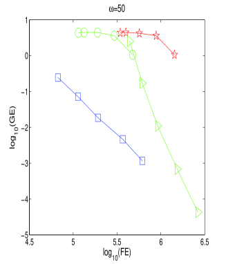
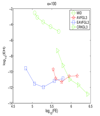
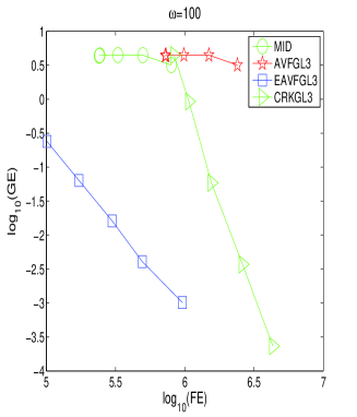
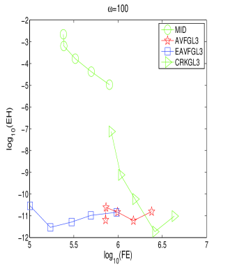
Figure 1. Efficiency curves.

Problem 5.2.

The equation

(35) $$\dot{x}_{1}=-\zeta x_{1}-\lambda x_{2}+x_{1}x_{2},$$

$$\dot{x}_{2}=\lambda x_{1}-\zeta x_{2}+\frac{1}{2}(x_{1}^{2}-x_{2}^{2}),$$

is an averaged system in wind-induced oscillation, where $\zeta\geq 0$ is a damping factor and $\lambda$ is a detuning parameter (see, e.g. [16]). For convenience, setting $\zeta=rcos(\theta),\lambda=rsin(\theta),r\geq 0,0\leq\theta\leq\pi/2$, (see [29]) we write (35) as

(36) $$\left(\begin{array}[]{c}\dot{x}_{1}\\ \dot{x}_{2}\end{array}\right)=\left(\begin{array}[]{cc}-cos(\theta)&-sin(\theta)\\ sin(\theta)&-cos(\theta)\end{array}\right)\left(\begin{array}[]{c}rx_{1}-\frac{1}{2}sin(\theta)(x_{2}^{2}-x_{1}^{2})-cos(\theta)x_{1}x_{2}\\ rx_{2}-sin(\theta)x_{1}x_{2}+\frac{1}{2}cos(\theta)(x_{2}^{2}-x_{1}^{2})\end{array}\right),$$

which is of the form (3), where

(37) $$Q=\left(\begin{array}[]{cc}-cos(\theta)&-sin(\theta)\\ sin(\theta)&-cos(\theta)\end{array}\right),\quad M=\left(\begin{array}[]{cc}r&0\\ 0&r\end{array}\right),\quad U=-\frac{1}{2}sin(\theta)(x_{1}x_{2}^{2}-\frac{1}{3}x_{1}^{3})+\frac{1}{2}cos(\theta)(\frac{1}{3}x_{2}^{3}-x_{1}^{2}x_{2}).$$

Its Lyapunov function (dissipative case, when $\theta<\pi/2$) or the first integral (conservative case, when $\theta=\pi/2$) is:

$$H=\frac{1}{2}r(x_{1}^{2}+x_{2}^{2})-\frac{1}{2}sin(\theta)(x_{1}x_{2}^{2}-\frac{1}{3}x_{1}^{3})+\frac{1}{2}cos(\theta)(\frac{1}{3}x_{2}^{3}-x_{1}^{2}x_{2}).$$

The matrix exponential of the EAVF scheme (13) for (36) are calculated by:

$$\exp(V)=\left(\begin{array}[]{cc}\exp(-hcr)cos(hsr)&-\exp(-hcr)sin(hsr)\\ \exp(-hcr)sin(hsr)&\exp(-hcr)cos(hsr)\end{array}\right),$$

where $c=cos(\theta),s=sin(\theta)$, and $\varphi(V)$ can be obtained by $(exp(V)-I)V^{-1}$. Given the initial values:

$$x_{1}(0)=0,x_{2}(0)=1,$$

we first integrate the conservative system (36) with the parameters $\theta=\pi/2,r=20$ and stepsizes $h=1/20\times 1/2^{i},i=-1,\ldots,4$ over the interval $[0,200]$. Setting $\theta=\pi/2-10^{-4},r=20,$ we then integrate the dissipative (36) with the stepsizes $h=1/20\times 1/2^{i},i=-1,\ldots,4$ over the interval $[0,100]$. Numerical errors are presented in Figs. 2, 3. It is noted that the integrands appearing in AVF, EAVF are polynomials of degree two and the integrands in CRK are polynomials of degree five. We evaluate the integrals in AVF, EAVF by the 2-point GL quadrature:

$$b_{1}=\frac{1}{2},b_{2}=\frac{1}{2},\quad c_{1}=\frac{1}{2}-\frac{3^{\frac{1}{2}}}{6},c_{2}=\frac{1}{2}+\frac{3^{\frac{1}{2}}}{6},$$

and the integrals appearing in CRK by the 3-point GL quadrature. Then there is no quadrature error.

The efficiency curves of AVF and MID consist of only five points in Figs. 2 (a), 2 (b), 3 (a) (two points overlap in Figs. 2 (a), 3 (a)), since the fixed-point iterations of MID and AVF are not convergent when $h=1/10$. Note that $QM$ is skew-symmetric or negative semi-definite, the convergence of iterations for the EAVF method is independent of $r$ by Theorem 3.2 and Remark 3.3. Thus larger stepsizes are allowed for EAVF. The experiment shows that the iterations of EAVF uniformly work for $h=1/20\times 1/2^{i},i=-1,\ldots,4$. Moreover, it can be observed from Fig. 2(d) that MID cannot strictly preserve the decay of the Lyapunov function.

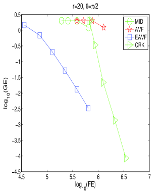
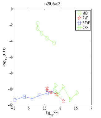
Figure 2. Efficiency curves.

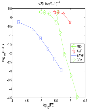
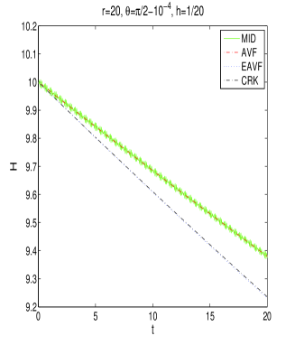
Figure 3. (a) Efficiency curves. (b) The Lyapunov function against time $t$.

Problem 5.3.

The PDE:

(38) $$\frac{\partial^{2}u}{\partial t^{2}}=\beta\frac{\partial^{3}u}{\partial t\partial x^{2}}+\frac{\partial^{2}u}{\partial x^{2}}\left(1+\varepsilon\left(\frac{\partial u}{\partial x}\right)^{p}\right)-\gamma\frac{\partial u}{\partial t}-m^{2}u,$$

where $\varepsilon>0,\beta,\gamma\geq 0$, is a continuous generalization of $\alpha$-FPU (Fermi-Pasta-Ulam) system (see, e.g. [27]). Taking $\partial_{t}u=v$ and the homogeneous Dirichlet BC $u(0,t)=u(L,t)=0$, the equation (38) is of the type (25), where $X=\mathbf{L}^{2}([0,L])\times\mathbf{L}^{2}([0,L])$ and

$$y=\left(\begin{array}[]{c}u\\ v\end{array}\right),\quad\mathcal{Q}=\left(\begin{array}[]{cc}0&1\\ -1&\beta\partial_{x}^{2}-\gamma\end{array}\right),\quad\mathcal{H}[y]=\int_{0}^{L}\left(\frac{1}{2}u_{x}^{2}+\frac{m^{2}}{2}u^{2}+\frac{v^{2}}{2}+\frac{\varepsilon u_{x}^{p+2}}{(p+2)(p+1)}\right)dx.$$

It is easy to verify that $\mathcal{Q}$ is a negative semi-definite operator, and thus (38) is dissipative. The spatial discretization yields a dissipative system of ODEs:

$$\ddot{u}_{j}(t)-c^{2}(u_{j-1}-2u_{j}+u_{j+1})+m^{2}u_{j}-\beta^{{}^{\prime}}(\dot{u}_{j-1}-2\dot{u}_{j}+\dot{u}_{j+1})+\gamma\dot{u}_{j}(t)=\varepsilon^{{}^{\prime}}(V^{{}^{\prime}}(u_{j+1}-u_{j})-V^{{}^{\prime}}(u_{j}-u_{j-1})),$$

where $c=1/\Delta x,\beta^{{}^{\prime}}=c^{2}\beta,\varepsilon^{{}^{\prime}}=c^{p+2}\varepsilon,V(u)=u^{p+2}/[(p+2)(p+1)],u_{j}(t)\approx u(x_{j},t),x_{j}=j/\Delta x$ for $j=1,\ldots,N-1$ and $u_{0}(t)=u_{N}(t)=0$. Note that the nonlinear term $u_{xx}u_{x}^{p}$ is approximated by :

$$\frac{\partial^{2}u}{\partial x^{2}}\left(\frac{\partial u}{\partial x}\right)^{p}|_{x=x_{j}}=\frac{1}{p+1}\partial_{x}\left(\frac{\partial u}{\partial x}\right)^{p+1}|_{x=x_{j}}\approx\frac{1}{p+1}\left(\left(\frac{u_{j+1}-u_{j}}{\Delta x}\right)^{p+1}-\left(\frac{u_{j}-u_{j-1}}{\Delta x}\right)^{p+1}\right)/\Delta x.$$

We now write it in the compact form (19):

$$\ddot{q}-N\dot{q}+\Omega q=-\nabla U_{1}(q),$$

where $q=(u_{1},\ldots,u_{N-1})^{\intercal},N=\beta^{{}^{\prime}}D-\gamma I,\Omega=-c^{2}D+m^{2}I,U_{1}(q)=\varepsilon^{{}^{\prime}}\sum_{j=0}^{N-1}V(u_{j+1}-u_{j})$ and

$$D=\left(\begin{array}[]{ccccc}-2&1&&&\\ 1&-2&1&&\\ &\ddots&\ddots&\ddots&\\ &&1&-2&1\\ &&&1&-2\end{array}\right).$$

In this experiment, we set $p=1,m=0,c=1,\varepsilon=\frac{3}{4},$ and $\gamma=0.005.$ Consider the initial conditions in [27]:

$$\phi_{j}(t)=B\ln\left\{\left(\frac{1+\exp[2(\kappa(j-97)+t\sinh(\kappa))]}{1+\exp[2(\kappa(j-96)+t\sinh(\kappa))]}\right)\left(\frac{1+\exp[2(\kappa(j-32)+t\sinh(\kappa))]}{1+\exp[2(\kappa(j-33)+t\sinh(\kappa))]}\right)\right\}$$

with $B=5,\kappa=0.1$, that is,

$$\left\{\begin{aligned} &u_{j}(0)=\phi_{j}(0),\\ &v_{j}(0)=\dot{\phi}_{j}(0).\\ \end{aligned}\right.$$

for $j=1,\ldots,N-1$. Let $N=128,\beta=0,2.$ We compute the numerical solution by MID, AVF and EAVF with the stepsizes $h=1/2^{i},i=1,\ldots,5$ over the time interval $[0,100]$. Similarly to EAVF (21), the nonlinear systems resulting from MID (31) and AVF (32) can be reduced to:

$$q^{1}=q^{0}+hp^{0}+\frac{h}{2}N(q^{1}-q^{0})-\frac{h^{2}}{4}\Omega(q^{1}+q^{0})-\frac{h^{2}}{2}\nabla U_{1}(\frac{q^{0}+q^{1}}{2}),$$

and

$$q^{1}=q^{0}+hp^{0}+\frac{h}{2}N(q^{1}-q^{0})-\frac{h^{2}}{4}\Omega(q^{1}+q^{0})-\frac{h^{2}}{2}\int_{0}^{1}\nabla U_{1}((1-\tau)q^{0}+\tau q^{1})d\tau$$

respectively. Both the velocity $p^{1}$ of MID and AVF can be recovered by

$$\frac{q^{1}-q^{0}}{h}=\frac{p^{1}+p^{0}}{2}.$$

The integrals in AVF and EAVF are exactly evaluated by the 2-point GL quadrature. Since $\exp(hA),\varphi(hA)$ in (21) have no explicit expressions, they are calculated by the Matlab package in [2]. The basic idea is evaluating $\exp(hA),\varphi(hA)$ by their Padé approximations. Numerical results are plotted in Figs. 4. Alternatively, there are other popular algorithms such as contour integral method and Krylov subspace method for matrix exponentials and $\varphi$-functions. Readers are referred to [23] for a summary of algorithms and well-established mathematical software.

According to Theorem 4.1, the convergence of iterations in the EAVF scheme is independent of $\Omega$ and $N$. Iterations of MID and AVF are not convergent when $\beta=2,h=1/2$. Thus the efficiency curves of MID and AVF in Fig. 4(b) consist of only $4$ points. From Fig. 4(c), it can be observed that the EAVF method can preserve dissipation even using the relatively large stepsize $h=1/2$.

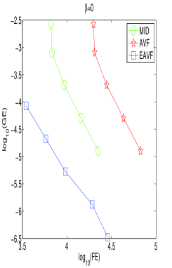
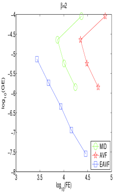
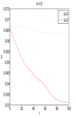
Figure 4. (a) (b) Efficiency curves. (c) The decay of Lyapunov function obtained by EAVF.

6. Conclusions

Exponential integrators can be traced back to the original paper by Hersch [20]. The term ‘exponential integrators’ was coined in the seminal paper by Hochbruck, Lubich and Selhofer [22]. It turns out that exponential integrators have constituted an important class of schemes for the numerical simulation of differential equations. In this paper, combining the ideas of the exponential integrator with the average vector field, we derived and analyzed a new exponential scheme EAVF preserving the first integral or the Lyapunov function for the conservative or dissipative system (3), which includes numerous important mathematical models in applications. The symmetry of EAVF ensures the prominent long-term numerical behavior. Due to the implicity of EAVF requires iteration solutions, we analysed the convergence of the fixed-point iteration and showed that the convergence is free from the influence of a wide range of coefficient matrices $M$. In the dynamics of the triatomic molecule, the wind-induced oscillation and the damped FPU problem, we compared the new EAVF method with the MID, AVF and CRK methods. The three problems are modeled by the system (3) having a dominant linear term and small nonlinear term. In the aspects of algebraic accuracy as well as preserving energy and dissipation, EAVF is very efficient among the four methods. In general, energy-preserving and energy-decaying methods are implicit, and then iteration solutions are required. With a relatively large stepsize, the iterations of EAVF are convergent, whereas AVF and MID do not work in experiments. Therefore, EAVF is expected to be a promising method solving the system (3) with $||QM||\gg||QHess(U)||$.

Acknowledgments.

The authors are sincerely thankful to two anonymous referees for their valuable suggestions, which help improve the presentation of the manuscript.

References

- [1] H. Berland, B. Owren, and B. Skaflestad, Solving the nonlinear Schrödinger equations using exponential integrators on the cubic Schrödinger equation, Model. Identif. Control 27 (2006) 201-217.
- [2] H. Berland, B. Skaflestad, and W. Wright, EXPINT – A MATLAB package for exponential integrators, ACM Transactions on Mathematical Software, 33 (2007).
- [3] L. Brugnano, F. Iavernaro, and D. Trigiante, Hamiltonan Boundary Value Methods (Energy Preserving Discrete Line Integral Methods), J. Numer. Anal. Ind. Appl. Math. 5 (2010) 13-17.
- [4] Projection methods preserving Lyapunov functions, BIT Numer. Math. 50 (2010) 223-241.
- [5] E. Celledoni, D. Cohen and B. Owren, Symmetric exponential integrators with an application to the cubic Schrödinger equation, Found. Comp. Math. 8 (2008) 303-317.
- [6] E. Celledoni, V. Grimm, R. I. Maclachlan, D. I. Maclaren, D. O’Neale, B. Owren, G. R. W. Quispel, Preserving energy resp. dissipation in numerical PDEs using the “Average Vector Field” method, J. Comput. Phys. 231 (2012) 6770-6789.
- [7] Jan L. Cieśliński, Locally exact modifications of numerical schemes, Computers&Mathematics with applications, 62 (2013) 1920-1938.
- [8] D. Cohen, Conservation properties of numerical integrators for highly oscillatory Hamiltonian systems, IMA Journal of Numerical Analysis 26 (2006) 34-59.
- [9] D. Cohen, T. Jahnke, K. Lorenz and C. Lubich, Numerical integrators for highly oscillatory Hamiltonian systems : A review. In Analysis, Modeling and Simulation of Multiscale Problems, (A. Mielke ed.), Springer (2006) 553-576.
- [10] S. M. Cox, P. C. Matthews, Exponential time differencing for stiff systems, J. Comput. Phys. 176 (2002) 430-455.
- [11] P. Deuflhard, A study of extrapolation methods based on multistep schemes without parasitic solutions, Z. Angew. Math. Phys. 30 (1979) 177-189.
- [12] J. Franco, Runge–Kutta–Nystrom methods adapted to the numerical integration of perturbed oscillators, Comput. Phys. Commun. 147 (2002) 770-787.
- [13] D. Furihata, T. Matuso, Discrete Variational Derivative Method : A Structure-Preserving Numerical Method for Partial Differential Equations, Chapman and Hall/CRC (2010).
- [14] W. Gautschi, Numerical integration of ordinary differential equations based on trigonometric polynomials, Numer. Math. 3 (1961) 381-397.
- [15] O. Gonzalez, Time Integration and Discrete Hamiltonian Systems, J. Nonlinear Sci. 6 (1996) 449-467.
- [16] J. Guckenheimer and P. Holmes, Nonlinear oscillations, Dynamical systems, and Bifurcations of vector fields, Springer–Verlag, New York, 1983.
- [17] E. Hairer, Energy-preserving variant of collocation methods, J. Numer. Anal. Ind. Appl. Math. 5 (2010) 73-84.
- [18] E. Hairer, C. Lubich, G. Wanner, Geometric Numerical Integration, 2nd edn. Springer, Berlin (2006) .
- [19] Y. Hernández-Solano, M. Atencia, G. Joya, F. Sandoval, A discrete gradient method to enhance the numerical behavior of Hopfield networks, Neurocomputing 164 (2015) 45-55.
- [20] J. Hersch, Contribution à la méthode des équations aux différences, Z. Angew. Math. Phys. 9 (1958) 129-180.
- [21] N. J. Higham, Functions of Matrices : Theory and Computation, SIAM, Philadelphia (2008).
- [22] M. Hochbruck, C. Lubich, H. Selhofer, Exponential integrators for large systems of differential equations, SIAM J. Sci. Comput. 19 (1998) 1552-1574.
- [23] M. Hochbruck, A. Ostermann, Exponential integrators, Acta Numerica (2010) 209-286.
- [24] A. K. Kassam, L. N. Trefethen, Fourth order time-stepping for stiff PDEs, SIAM. J. Sci. Comput. 26 (2005) 1214-1233.
- [25] C. Klein, Fourth order time-stepping for low dispersion Kortewerg–de Vries and nonlinear Schrödinger equations, Electron. Trans. Numer. Anal. 29 (2008) 116-135.
- [26] J. D. Lawson, Generalized Runge–Kutta processes for stable systems with large Lipschitz constants, SIAM. J. Numer. Anal. Model. 6 (1967) 642-659.
- [27] J. E. Macías–Díaz, I. E. Medina–Ramírez, An implicit four-step computational method in the study on the effects of damping in a modified –Fermi–Pasta–Ulam medium, Commun. Nonlinear Sci. Numer. Simulat. 14 (2009) 3200-3212.
- [28] R. I. Maclachlan, G. R. W Quispel, and N. Robidoux, Geometric Integration Using Dicrete Gradients, Philos. Trans. R. Soc. A 357 (1999) 1021-1046.
- [29] R. I. Maclachlan, G. R. W Quispel, and N. Robidoux, A unified approach to Hamiltonian systems, Poisson systems, gradient systems, and systems with Lyapunov functions or first integrals, Phys. Rev. Lett. 81 (1998) 2399-2411.
- [30] B.V. Pavlov, O. E. Rodionova, The method of local linearization in the numerical solution of stiff systems of ordinary differential equations, USSR Computational Mathematics and Mathemaitcal Physics, 27 (1987) 30-38.
- [31] B. Wang, X. Wu, A new high presicion energy-preserving integrator for system of oscillatory second-order differential equations, Physics Letters A 376 (2012) 1185-1190.
- [32] X. Wu, B. Wang, Xia, J., Explicit symplectic multidimensional exponential fitting modified Runge–Kutta–Nystrom methods, BIT Numer. Math. 52 (2012) 773-791.
- [33] H. Yang, X. Wu, X. You, Y. Fang, Extended RKN-type methods for numerical integration of perturbed oscillators, Comput. Phys. Commun. 180 (2009) 1777-1794.