Functionally-fitted energy-preserving methods for solving oscillatory nonlinear Hamiltonian systems

Abstract.

In the last few decades, numerical simulation for nonlinear oscillators has received a great deal of attention, and many researchers have been concerned with the design and analysis of numerical methods for solving oscillatory problems. In this paper, from the perspective of the continuous finite element method, we propose and analyze new energy-preserving functionally fitted methods, in particular trigonometrically fitted methods of an arbitrarily high order for solving oscillatory nonlinear Hamiltonian systems with a fixed frequency. To implement these new methods in a widespread way, they are transformed into a class of continuous-stage Runge–Kutta methods. This paper is accompanied by numerical experiments on oscillatory Hamiltonian systems such as the FPU problem and nonlinear Schrödinger equation. The numerical results demonstrate the remarkable accuracy and efficiency of our new methods compared with the existing high-order energy-preserving methods in the literature.

1. Introduction

In this paper, we consider nonlinear Hamiltonian systems:

(1) $$y^{\prime}(t)=f(y(t))=J^{-1}\nabla H(y(t)),\quad y(t_{0})=y_{0}\in\mathbb{R}^{d},$$

where $d=2d_{1},f:\mathbb{R}^{d}\rightarrow\mathbb{R}^{d},H:\mathbb{R}^{d}\rightarrow\mathbb{R}$ are sufficiently smooth functions and

$$J=\left(\begin{array}[]{cc}O_{d_{1}\times d_{1}}&I_{d_{1}\times d_{1}}\\ -I_{d_{1}\times d_{1}}&O_{d_{1}\times d_{1}}\end{array}\right)$$

is the canonical symplectic matrix. It is well known that the flow of (1) preserves the symplectic form $dy\wedge Jdy$ and the Hamiltonian or energy $H(y(t))$. In the spirit of geometric numerical integration, it is a natural idea to design schemes that preserve both the symplecticity of the flow and Hamiltonian function. Unfortunately, a numerical scheme cannot achieve this goal unless it generates the exact solution (see, e.g. [21], page 379). Hence researchers face a choice between preserving symplecticity or energy and many of them have given more weight on the former in the last decades, and readers are referred to [21] and references therein. Whereas investigations on energy-preserving (EP) methods are relatively insufficient (see, e.g. [1, 4, 6, 10, 11, 16, 18, 22, 26, 35]). Comparing to symplectic methods, EP methods are beneficial for improving nonlinear stability, easier to adapt the time step and more suitable for the integration of chaotic systems (see, e.g. [12, 19, 32, 34]).

On the other hand, in scientific computing and modelling, the design and analysis of methods for periodic or oscillatory systems have been considered by many authors (see, e.g. [2, 17, 20, 31, 38, 41]). Generally, these methods utilize a priori information of special problems and they are more efficient than general-purpose methods. A popular approach to constructing methods suitable for oscillatory problems is using the functionally-fitted (FF) condition, namely, deriving a suitable method by requiring it to integrate members of a given finite-dimensional function space $X$ exactly. If $X$ incorporates trigonometrical or exponential functions, the corresponding methods are also named by trigonometrically-fitted (TF) or exponentially-fitted (EF) methods (see, e.g. [14, 25, 29, 33]).

Therefore, combining the ideas of the EF/TF and structure-preserving methods is a promising approach to developing numerical methods which allow long-term computation of solutions to oscillatory Hamiltonian systems (1). Just as the research of symplectic and EP methods, EF/TF symplectic methods have been studied extensively by many authors (see, e.g. [7, 8, 9, 15, 36, 37, 40]). By contrast, as far as we know, only a few papers paid attention to the EF/TF EP methods (see, e.g. [27, 28, 39]). Usually the existing EF/TF EP methods are derived in the context of continuous-stage Runge–Kutta (RK) methods. The coefficients in these methods are determined by a system of equations resulting from EF/TF, EP and symmetry conditions. As mentioned at the end of [27], it is not easy to find such a system having a unique solution in the case of deriving high-order methods. What’s more, how to verify the algebraic order of such methods falls into a question. A common way is to check order conditions related to rooted trees. Again, this is inconvenient in the high-order setting since the number of trees increases extremely fast as the order grows. In this paper, we will construct FF EP methods based on the continuous finite element method, which is inherently energy-preserving (see, e.g. [1, 16, 35]). Intuitively, we are expected to increase the order of the method through enlarging the finite element space. By adding trigonometrical functions to the space, the corresponding method is naturally trigonometrically fitted. Thus we are hopeful of constructing FF EP methods, in particular TF EP methods, of arbitrarily high order.

The outline of this paper is as follows. In Section 2, we construct FF CFE methods and present important geometric properties of them. In Section 3, we interpret them as continuous-stage Runge–Kutta methods and analyse the algebraic order. We then discuss implementation details of these new methods in Section 4. Numerical results are shown in section 5, including the comparison between our new TF EP methods and other prominent structure-preserving methods in the literature. The last section is concerned with the conclusion and discussion.

2. Functionally-fitted continuous finite element methods for Hamiltonian systems

Preliminaries 2.1.

Throughout this paper, we consider the IVP (1) on the time interval $I=[t_{0},T]$, which is equally partitioned into $t_{0}<t_{1}<\ldots<t_{N}=T$, with $t_{n}=t_{0}+nh$ for $n=0,1,\ldots,N$. A function space $Y$=span$\left\{\varphi_{0},\ldots,\varphi_{r-1}\right\}$ means that

$$Y=\left\{w:w(t)=\sum_{i=0}^{r-1}W_{i}\varphi_{i}(t),W_{i}\in\mathbb{R}^{d}\right\}.$$

Here, $\{\varphi_{i}\}_{i=0}^{r-1}$ are supposed to be sufficiently smooth and linearly independent on $I$. A function $w$ on $I$ is called a piecewise $Y$-type function if for any $0\leq n\leq N-1$, there exists a function $g\in Y$, such that $w|_{(t_{n},t_{n+1})}=g|_{(t_{n},t_{n+1})}.$

Sometimes, it is convenient to introduce the transformation $t=t_{0}+\tau h$ for $\tau\in[0,1]$. Accordingly we denote $Y_{h}(t_{0})=\left\{v\text{ on }[0,1]:v(\tau)=w(t_{0}+\tau h),w\in Y\right\}$. Hence $Y_{h}(t_{0})$=span$\left\{\tilde{\varphi}_{0},\ldots,\tilde{\varphi}_{r-1}\right\}$, where $\tilde{\varphi}_{i}(\tau)=\varphi_{i}(t_{0}+\tau h)$ for $i=0,1,\ldots,r-1$. In what follows, lowercase Greek letters such as $\tau,\sigma,\alpha$ always indicate variables on the interval [0,1] unless confusions arise.

Given two integrable functions (scalar-valued or vector-valued) $w_{1}$ and $w_{2}$ on $[0,1]$, the inner product $\langle\cdot,\cdot\rangle$ is defined by

$$\langle w_{1},w_{2}\rangle=\langle w_{1}(\tau),w_{2}(\tau)\rangle_{\tau}=\int_{0}^{1}w_{1}(\tau)\cdot w_{2}(\tau)d\tau,$$

where $\cdot$ is the entrywise multiplication operation if $w_{1},w_{2}$ are both vector-valued functions of the same length.

Given two finite-dimensional function spaces $X$ and $Y$ whose members are $\mathbb{R}^{d}$-valued, the continuous finite element method for (1) is described as follows.

Find a continuous piecewise X-type function $U(t)$ on $I$ with $U(t_{0})=y_{0}$, such that

(2) $$\int_{I}v(t)\cdot(U^{\prime}(t)-f(U(t)))dt=0,$$

for any piecewise Y-type function $v(t)$, where $U(t)\approx y(t)$ on $I$ and $y(t)$ solves the IVP (1). The term ‘continuous finite element’(CFE) comes from the continuity of the finite element solution $U(t)$. Since (2) deals with an initial value problem, we need only to consider it on $[t_{0},t_{0}+h]$.

Find $u\in X_{h}(t_{0})$ with $u(0)=y_{0}$, such that

(3) $$\langle v,u^{\prime}\rangle=h\langle v,f\circ u\rangle,$$

for any $v\in Y_{h}(t_{0})$, where

$$u(\tau)=U(t_{0}+\tau h)\approx y(t_{0}+\tau h)$$

for $\tau\in[0,1]$. Since $U(t)$ is continuous, $y_{1}=u(1)$ is the initial value of the local problem on the next interval $[t_{1},t_{2}]$. Thus we can solve the global variational problem (2) on $I$ step by step.

In the special case of

$$X=\text{span}\left\{1,t,\ldots,t^{r}\right\},\quad Y=\text{span}\left\{1,t,\ldots,t^{r-1}\right\},$$

(2) reduces to the classical continuous finite element method (see, e.g. [1, 24]) denoted by CFE$r$ in this paper. For the purpose of deriving functionally-fitted methods, we generalize $X$ and $Y$ a little:

(4) $$Y=\text{span}\left\{\varphi_{0}(t),\ldots,\varphi_{r-1}(t)\right\},\quad X=\text{span}\left\{1,\int_{t_{0}}^{t}\varphi_{0}(s)ds,\ldots,\int_{t_{0}}^{t}\varphi_{r-1}(s)ds\right\}.$$

Thus it is sufficient to give $X$ or $Y$ since they can be determined by each other. Besides, $Y$ is supposed to be invariant under translation and reflection , namely,

(5) $$v(t)\in Y\Rightarrow v(t+c)\in Y\text{ for any }c\in\mathbb{R},$$

$$v(t)\in Y\Rightarrow v(-t)\in Y.$$

Clearly, $Y_{h}(t_{0})$ and $X_{h}(t_{0})$ are irrelevant to $t_{0}$ provided (5) holds. For convenience, we simplify $Y_{h}(t_{0})$ and $X_{h}(t_{0})$ by $Y_{h}$ and $X_{h}$ respectively. In the remainder of this paper, we denote the CFE method (2) or (3) based on the general function spaces (4) satisfying the condition (5) by FFCFE$r$.

It is noted that the FFCFE$r$ method (3) is defined by a variational problem and the well-definedness of this problem has not been confirmed yet. Here we presume the existence and uniqueness of the solution to (3). This assumption will be proved in the next section. With this premise, we are able to present three significant properties of the FFCFE$r$ method. At first, by the definition of the variational problem (2), the FFCFE$r$ method is functionally fitted with respect to the space $X$.

Theorem 2.2.

The FFCFE$r$ method (2) solves the IVP (1) whose solution is a piecewise $X$-type function without any error.

Moreover, the FFCFE$r$ method is inherently energy preserving method. The next theorem confirms this point.

Theorem 2.3.

The FFCFE$r$ method (3) exactly preserves the Hamiltonian $H$: $H(y_{1})=H(y_{0})$.

Proof.

Firstly, given a vector $V$, its $i$th entry is denoted by $V_{i}$. For each function $w\in Y_{h}$, setting $v(\tau)=w(\tau)\cdot e_{i}\in Y_{h}$ in (3) leads to

$$\int_{0}^{1}w(\tau)_{i}u^{\prime}(\tau)_{i}d\tau=h\int_{0}^{1}w(\tau)_{i}f(u(\tau))_{i}d\tau,\quad i=1,2,\ldots,d,$$

where $e_{i}$ is the $i$th vector of units. Thus

(6) $$\int_{0}^{1}w(\tau)^{\intercal}u^{\prime}(\tau)d\tau=\sum_{i=1}^{d}\int_{0}^{1}w(\tau)_{i}u^{\prime}(\tau)_{i}d\tau$$

$$=\sum_{i=1}^{d}h\int_{0}^{1}w(\tau)_{i}f(u(\tau))_{i}d\tau=h\int_{0}^{1}w(\tau)^{\intercal}f(u(\tau))d\tau.$$

Since $u(\tau)\in X_{h}$, $u^{\prime}(\tau)\in Y_{h}$ and $J^{-1}u^{\prime}(\tau)\in Y_{h}$, by taking $w(\tau)=J^{-1}u^{\prime}(\tau)$ in (6), we have

$$H(y_{1})-H(y_{0})$$

$$=\int_{0}^{1}\frac{d}{d\tau}H(u(\tau))d\tau=\int_{0}^{1}u^{\prime}(\tau)^{\intercal}\nabla H(u(\tau))d\tau$$

$$=\int_{0}^{1}(J^{-1}u^{\prime}(\tau))^{\intercal}f(u(\tau))d\tau=h^{-1}\int_{0}^{1}u^{\prime}(\tau)^{\intercal}Ju^{\prime}(\tau)d\tau=0.$$

This completes the proof.∎

∎

The FFCFE$r$ method can also be viewed as a one-step method $\Phi_{h}:y_{0}\rightarrow y_{1}=u(1)$. It is well known that reversible methods show a better long-term behaviour than nonsymmetric ones when applied to reversible differential systems such as (1) (see, e.g. [21]). This fact motivates the investigation of the symmetry of the FFCFE$r$ method. Since spaces $X$ and $Y$ satisfy the invariance (5), which is a kind of symmetry, the FFCFE$r$ method is expected to be symmetric.

Theorem 2.4.

The FFCFE$r$ method (3) is symmetric provided (5) holds.

Proof.

According to (5), we have $X_{h}=X_{-h},Y_{h}=Y_{-h}.$ Exchanging $y_{0}\leftrightarrow y_{1}$ and replacing $h$ with $-h$ in (3) give: $u(0)=y_{1}$, $y_{0}=u(1)$, where

$$\langle v(\tau),u^{\prime}(\tau)\rangle_{\tau}=-h\langle v(\tau),f(u(\tau))\rangle_{\tau},\quad u(\tau)\in X_{-h}=X_{h},$$

for each $v(\tau)\in Y_{-h}=Y_{h}$. Setting $u_{1}(\tau)=u(1-\tau)\in X_{h}$ and $\tau\to 1-\tau$ leads to $u_{1}(0)=y_{0}$, $y_{1}=u_{1}(1)$, where

$$\langle v_{1}(\tau),u_{1}^{\prime}(\tau)\rangle_{\tau}=h\langle v_{1}(\tau),f(u_{1}(\tau))\rangle_{\tau},$$

for each $v_{1}(\tau)=v(1-\tau)\in Y_{h}.$ This method is exactly the same as (3), which means that the FFCFE$r$ method is symmetric. ∎

∎

It is well known that polynomials cannot approximate oscillatory functions satisfactorily. If the problem (1) has a fixed frequency $\omega$ which can be evaluated effectively in advance, then the function space containing the pair $\left\{\sin(\omega t),\cos(\omega t)\right\}$ seems to be a more promising candidate for $X$ and $Y$ than the polynomial space. For example, possible $Y$ spaces for deriving the TF CFE method are

(7) $$Y_{1}=\left\{\begin{aligned} &\text{span}\left\{\cos(\omega t),\sin(\omega t)\right\},r=2,\\ &\text{span}\left\{1,t,\ldots,t^{r-3},\cos(\omega t),\sin(\omega t)\right\},r\geq 3,\\ \end{aligned}\right.$$

(8) $$Y_{2}=\text{span}\left\{\cos(\omega t),\sin(\omega t),\ldots,\cos(k\omega t),\sin(k\omega t)\right\},r=2k,$$

and

(9) $$Y_{3}=\text{span}\left\{1,t,\ldots,t^{p},t\cos(\omega t),t\sin(\omega t),\ldots,t^{k}\cos(\omega t),t^{k}\sin(\omega t)\right\}.$$

Correspondingly, by equipping the FF CFE method with the space $Y=Y_{1},Y_{2}$ or $Y_{3}$, we obtain three families of TF CFE methods. According to Theorem 2.3 and Theorem 2.4, all of them are symmetric energy-preserving methods. To exemplify this framework of the TF CFE method, in numerical experiments, we will test the TF CFE method denoted by TFCFE$r$ and TF2CFE$r$ based on the spaces (7) and (8). It is noted that TFCFE2 and TF2CFE2 coincide.

3. Interpretation as continuous-stage Runge–Kutta methods and the analysis on the algebraic order

An interesting connection between CFE methods and RK-type methods has been shown in a few papers (see, e.g. [3, 24, 35]). Since the RK methods are dominant in the numerical integration of ODEs, it is meaningful and useful to transform the FFCFE$r$ method to the corresponding RK-type method which has been widely and conventionally used in applications. After the transformation, the FFCFE$r$ method can be analysed and implemented by standard techniques in ODEs conveniently. To this end, it is helpful to introduce the projection operation $P_{h}$. Given a continuous $\mathbb{R}^{d}$-valued function $w$ on $[0,1]$, its projection onto $Y_{h}$, denoted by $P_{h}w$, is defined by

(10) $$\langle v,P_{h}w\rangle=\langle v,w\rangle,\quad\text{for any }v\in Y_{h}.$$

Clearly, $P_{h}w(\tau)$ can be uniquely expressed as a linear combination of $\{\tilde{\varphi}_{i}(\tau)\}_{i=0}^{r-1}$:

$$P_{h}w(\tau)=\sum_{i=0}^{r-1}U_{i}\tilde{\varphi}_{i}(\tau),\quad U_{i}\in\mathbb{R}^{d}.$$

Taking $v(\tau)=\tilde{\varphi}_{i}(\tau)e_{j}$ in (10) for $i=0,1,\ldots,r-1$ and $j=1,\ldots,d$, it can be observed that coefficients $U_{i}$ satisfy the equation

$$M\otimes I_{d\times d}\left(\begin{array}[]{c}U_{0}\\ \vdots\\ U_{r-1}\end{array}\right)=\left(\begin{array}[]{c}\langle\tilde{\varphi}_{0},w\rangle\\ \vdots\\ \langle\tilde{\varphi}_{r-1},w\rangle\end{array}\right),$$

where

$$M=(\langle\tilde{\varphi}_{i},\tilde{\varphi}_{j}\rangle)_{0\leq i,j\leq r-1}.$$

Since $\left\{\tilde{\varphi}_{i}\right\}_{i=0}^{r-1}$ are linearly independent for $h>0$, the stiffness matrix $M$ is nonsingular. Thus the projection can be explicitly expressed by

$$P_{h}w(\tau)=\langle P_{\tau,\sigma},w(\sigma)\rangle_{\sigma},$$

where

(11) $$P_{\tau,\sigma}=(\tilde{\varphi}_{0}(\tau),\ldots,\tilde{\varphi}_{r-1}(\tau))M^{-1}(\tilde{\varphi}_{0}(\sigma),\ldots,\tilde{\varphi}_{r-1}(\sigma))^{\intercal}.$$

Clearly, $P_{\tau,\sigma}$ can be calculated by a basis other than $\left\{\tilde{\varphi}_{i}\right\}_{i=0}^{r-1}$ since they only differ in a linear transformation. If $\left\{\phi_{0},\ldots,\phi_{r-1}\right\}$ is an orthonormal basis of $X_{h}$ under the inner product $\langle\cdot,\cdot\rangle$, then $P_{\tau,\sigma}$ admits a simpler expression:

(12) $$P_{\tau,\sigma}=\sum_{i=0}^{r-1}\phi_{i}(\tau)\phi_{i}(\sigma).$$

Now using (3) and the definition (10) of the operator $P_{h}$, we obtain that $u^{\prime}=hP_{h}(f\circ u)$ and

(13) $$u^{\prime}(\tau)=h\langle P_{\tau,\sigma},f(u(\sigma))\rangle_{\sigma}.$$

Integrating the above equation with respect to $\tau$, we transform the FFCFE$r$ method (3) into the continuous-stage RK method:

(14) $$\left\{\begin{aligned} &u(\tau)=y_{0}+h\int_{0}^{1}A_{\tau,\sigma}f(u(\sigma))d\sigma,\\ &y_{1}=u(1),\\ \end{aligned}\right.$$

where

(15) $$A_{\tau,\sigma}=\int_{0}^{\tau}P_{\alpha,\sigma}d\alpha=\sum_{i=0}^{r-1}\int_{0}^{\tau}\phi_{i}(\alpha)d\alpha\phi_{i}(\sigma).$$

In particular,

(16) $$\phi_{i}(\tau)=\hat{p}_{i}(\tau),$$

for the CFE$r$ method for $i=0,1,\ldots,r-1$, where $\hat{p}_{i}(\tau)$ is the shifted Legendre polynomial of degree $i$ on $[0,1]$, scaled in order to be orthonormal. Thus the CFE$r$ method in the form (14) is identical to the energy-preserving collocation method of order $2r$ (see [22]) or the Hamiltonian boundary value method HBVM$(\infty,r)$ (see, e.g. [4]). For the FFCFE$r$ method, since $P_{\tau,\sigma},A_{\tau,\sigma}$ are functions of variable $h$ and $u(\tau)$ is implicitly determined by (14), it is necessary to analyse their smoothness with respect to $h$ before investigating the analytic property of the numerical solution $u(\tau)$. First of all, it can be observed from (11) that $P_{\tau,\sigma}=P_{\tau,\sigma}(h)$ is not defined at $h=0$ since the matrix $M$ is singular in this case. Fortunately, the following lemma shows that the singularity is removable.

Lemma 3.1.

When $h$ tends to 0, the limit of $P_{\tau,\sigma}$ there exists. What’s more, $P_{\tau,\sigma}$ can be smoothly extended to $h=0$ by setting $P_{\tau,\sigma}(0)=\lim_{h\to 0}P_{\tau,\sigma}(h)$.

Proof.

By expanding $\{\varphi_{i}(t_{0}+\tau h)\}_{i=0}^{r-1}$ at $t_{0}$, we obtain that

(17) $$(\tilde{\varphi}_{0}(\tau),\ldots,\tilde{\varphi}_{r-1}(\tau))=(1,\tau h,\ldots,\frac{\tau^{r-1}h^{r-1}}{(r-1)!})W+\mathcal{O}(h^{r}),$$

where

(18) $$W=\left(\begin{array}[]{cccc}\varphi_{0}(t_{0})&\varphi_{1}(t_{0})&\cdots&\varphi_{r-1}(t_{0})\\ \varphi_{0}^{(1)}(t_{0})&\varphi_{1}^{(1)}(t_{0})&\cdots&\varphi_{r-1}^{(1)}(t_{0})\\ \vdots&\vdots&&\vdots\\ \varphi_{0}^{(r-1)}(t_{0})&\varphi_{1}^{(r-1)}(t_{0})&\cdots&\varphi_{r-1}^{(r-1)}(t_{0})\end{array}\right)$$

is the Wronskian of $\{\varphi_{i}(t)\}_{i=0}^{r-1}$ at $t_{0}$, which is nonsingular. Post-multiplying the right-hand side of (17) by $W^{-1}diag(1,h^{-1},\ldots,h^{1-r}(r-1)!)$ yields another basis of $X_{h}$:

$$\{1+\mathcal{O}(h),\tau+\mathcal{O}(h),\ldots,\tau^{r-1}+\mathcal{O}(h)\}.$$

Applying the Gram-Schmidt process (with respect to the inner product $\langle\cdot,\cdot\rangle$) to the above basis, we obtain an orthonormal basis $\left\{\phi_{i}(\tau)=\hat{p}_{i}(\tau)+\mathcal{O}(h)\right\}_{i=0}^{r-1}$. Thus by (12) and defining

(19) $$P_{\tau,\sigma}(0)=\lim_{h\to 0}\sum_{i=0}^{r-1}\phi_{i}(\tau)\phi_{i}(\sigma)=\sum_{i=0}^{r-1}\hat{p}_{i}(\tau)\hat{p}_{i}(\sigma),$$

$P_{\tau,\sigma}$ is extended to $h=0$. Since each $\phi_{i}(\tau)=\hat{p}_{i}(\tau)+\mathcal{O}(h)$ is smooth with respect to $h$, $P_{\tau,\sigma}$ is also a smooth function of $h$. ∎

∎

From (16) and (19), it can be observed that the FFCFE$r$ method (14) reduces to the CFE$r$ method when $h\to 0$, or equivalently, the energy-preserving collocation method of order $2r$ and HBVM$(\infty,r)$ method mentioned above. Since $A_{\tau,\sigma}=\int_{0}^{\tau}P_{\alpha,\sigma}d\alpha$ is also a smooth function of $h$, we can assume that

(20) $$M_{k}=\max_{\tau,\sigma,h\in[0,1]}\left|\frac{\partial^{k}A_{\tau,\sigma}}{\partial h^{k}}\right|,\quad k=0,1,\ldots.$$

Furthermore, since the right function $f$ in (1) maps from $\mathbb{R}^{d}$ to $\mathbb{R}^{d}$, the $n$th-order derivative of $f$ at $y$ denoted by $f^{(n)}(y)$ is a multilinear map from $\underbrace{\mathbb{R}^{d}\times\ldots\times\mathbb{R}^{d}}_{n-fold}$ to $\mathbb{R}^{d}$ defined by

$$f^{(n)}(y)(z_{1},\ldots,z_{n})=\sum_{1\leq\alpha_{1},\ldots,\alpha_{n}\leq d}\frac{\partial^{n}f}{\partial y_{\alpha_{1}}\cdots\partial y_{\alpha_{n}}}(y)z_{1}^{\alpha_{1}}\ldots z_{n}^{\alpha_{n}},$$

where $y=(y_{1},\ldots,y_{d})^{\intercal}$ and $z_{i}=(z_{i}^{1},\ldots,z_{i}^{d})^{\intercal}$, $i=1,\ldots,n$. With this background, we now can give the existence, uniqueness, especially the smoothness with respect to $h$ for the continuous finite element approximation $u(\tau)$ associated with the FFCFE$r$ method. The proof of the following theorem is based on a fixed-point iteration which is analogous to Picard iteration.

Theorem 3.2.

Given a positive constant $R$, let

$$B(y_{0},R)=\left\{y\in\mathbb{R}^{d}:||y-y_{0}||\leq R\right\}$$

and

(21) $$D_{n}=\max_{y\in B(y_{0},R)}||f^{(n)}(y)||,\quad n=0,1,\ldots,$$

where $||\cdot||=||\cdot||_{\infty}$ is the maximum norm for vectors in $\mathbb{R}^{d}$ or the corresponding induced norm for the multilinear maps $f^{(n)}(y),n\geq 1$. Then the FFCFE$r$ method (3) or (14) has a unique solution $u(\tau)$ which is smoothly dependent of $h$ provided

(22) $$0\leq h\leq\varepsilon<\min\left\{\frac{1}{M_{0}D_{1}},\frac{R}{M_{0}D_{0}},1\right\}.$$

Proof.

Set $u_{0}(\tau)\equiv y_{0}$. We construct a function series $\{u_{n}(\tau)\}_{n=0}^{\infty}$ defined by the relation

(23) $$u_{n+1}(\tau)=y_{0}+h\int_{0}^{1}A_{\tau,\sigma}f(u_{n}(\sigma))d\sigma,{\quad n=0,1,\ldots.}$$

Obviously, $\lim_{n\to\infty}u_{n}(\tau)$ is a solution to (14) provided $\left\{u_{n}(\tau)\right\}_{n=0}^{\infty}$ is uniformly convergent. Thus we need only to prove the uniform convergence of the infinite series

$$\sum_{n=0}^{\infty}(u_{n+1}(\tau)-u_{n}(\tau)).$$

It follows from (20), (22), (23) and induction that

(24) $$||u_{n}(\tau)-y_{0}||\leq R,\quad n=0,1,\ldots$$

Then by using (21), (22), (23), (24) and the inequalities

$$||\int_{0}^{1}w(\tau)d\tau||\leq\int_{0}^{1}||w(\tau)||d\tau,\quad\text{for $\mathbb{R}^{d}$-valued function $w(\tau)$},$$

$${||f(y)-f(z)||\leq D_{1}||y-z||,\quad\text{for }y,z\in B(y_{0},R),}$$

we obtain the following inequalities

$$||u_{n+1}(\tau)-u_{n}(\tau)||\leq h\int_{0}^{1}M_{0}D_{1}||u_{n}(\sigma)-u_{n-1}(\sigma)||d\sigma$$

$$\leq\beta||u_{n}-u_{n-1}||_{c},\quad{\beta=\varepsilon M_{0}D_{1},}$$

where $||\cdot||_{c}$ is the maximum norm for continuous functions:

$$||w||_{c}=\max_{\tau\in[0,1]}||w(\tau)||,\quad\text{$w$ is a continuous $\mathbb{R}^{d}$-valued function on $[0,1]$}.$$

Thus, we have

$$||u_{n+1}-u_{n}||_{c}\leq\beta||u_{n}-u_{n-1}||_{c}$$

and

(25) $$||u_{n+1}-u_{n}||_{c}\leq\beta^{n}||u_{1}-y_{0}||_{c}\leq\beta^{n}R,\quad n=0,1,\ldots.$$

Since $\beta<1$, according to Weierstrass $M$-test, $\sum_{n=0}^{\infty}(u_{n+1}(\tau)-u_{n}(\tau))$ is uniformly convergent, and thus, the limit of $\{u_{n}(\tau)\}_{n=0}^{\infty}$ is a solution to (14). If $v(\tau)$ is another solution, then the difference between $u(\tau)$ and $v(\tau)$ satisfies

$$||u(\tau)-v(\tau)||\leq h\int_{0}^{1}||A_{\tau,\sigma}(f(u(\sigma))-f(v(\sigma)))||d\sigma\leq\beta||u-v||_{c},$$

and

$$||u-v||_{c}\leq\beta||u-v||_{c}.$$

This means $||u-v||_{c}=0,$ i.e., $u(\tau)\equiv v(\tau)$. Hence the existence and uniqueness have been proved.

As for the smooth dependence of $u$ on $h$, since every $u_{n}(\tau)$ is a smooth function of $h$, we need only to prove the series

$$\left\{\frac{\partial^{k}u_{n}}{\partial h^{k}}(\tau)\right\}_{n=0}^{\infty}$$

are uniformly convergent for $k\geq 1$. Firstly, differentiating both sides of (23) with respect to $h$ yields

(26) $$\frac{\partial u_{n+1}}{\partial h}(\tau)=\int_{0}^{1}(A_{\tau,\sigma}+h\frac{\partial A_{\tau,\sigma}}{\partial h})f(u_{n}(\sigma))d\sigma+h\int_{0}^{1}A_{\tau,\sigma}f^{(1)}(u_{n}(\sigma))\frac{\partial u_{n}}{\partial h}(\sigma)d\sigma.$$

We then have

(27) $$||\frac{\partial u_{n+1}}{\partial h}||_{c}\leq\alpha+\beta||\frac{\partial u_{n}}{\partial h}||_{c},\quad\alpha=(M_{0}+\varepsilon M_{1})D_{0}.$$

By induction, it is easy to show that $\left\{\frac{\partial u_{n}}{\partial h}(\tau)\right\}_{n=0}^{\infty}$ is uniformly bounded:

(28) $$||\frac{\partial u_{n}}{\partial h}||_{c}\leq\alpha(1+\beta+\ldots+\beta^{n-1})\leq\frac{\alpha}{1-\beta}=C^{*},\quad n=0,1,\ldots.$$

Combining (25), (26) and (28), we obtain

$$||\frac{\partial u_{n+1}}{\partial h}-\frac{\partial u_{n}}{\partial h}||_{c}$$

$$\leq\int_{0}^{1}(M_{0}+hM_{1})||f(u_{n}(\sigma))-f(u_{n-1}(\sigma))||d\sigma$$

$$+h\int_{0}^{1}M_{0}\left(||(f^{(1)}(u_{n}(\sigma))-f^{(1)}(u_{n-1}(\sigma)))\frac{\partial u_{n}}{\partial h}(\sigma)||+||f^{(1)}(u_{n-1}(\sigma))(\frac{\partial u_{n}}{\partial h}(\sigma)-\frac{\partial u_{n-1}}{\partial h}(\sigma))||\right)d\sigma$$

$$\leq\gamma\beta^{n-1}+\beta||\frac{\partial u_{n}}{\partial h}-\frac{\partial u_{n-1}}{\partial h}||_{c},$$

where

$$\gamma=(M_{0}D_{1}+\varepsilon M_{1}D_{1}+\varepsilon M_{0}L_{2}C^{*})R,$$

and $L_{2}$ is a constant satisfying

$$||f^{(1)}(y)-f^{(1)}(z)||\leq L_{2}||y-z||,\quad\text{for $y,z\in B(y_{0},R)$}.$$

Thus again by induction, we have

$$||\frac{\partial u_{n+1}}{\partial h}-\frac{\partial u_{n}}{\partial h}||_{c}\leq n\gamma\beta^{n-1}+\beta^{n}C^{*},\quad n=1,2,\ldots$$

and $\left\{\frac{\partial u_{n}}{\partial h}(\tau)\right\}_{n=0}^{\infty}$ is uniformly convergent. By a similar argument, one can show that other function series $\left\{\frac{\partial^{k}u_{n}}{\partial h^{k}}(\tau)\right\}_{n=0}^{\infty}$ for $k\geq 2$ are uniformly convergent as well. Therefore, $u(\tau)$ is smoothly dependent on $h$. The proof is complete. ∎

∎

Since our analysis on the algebraic order of the FFCFE$r$ method is mainly based on Taylor’s theorem, it is meaningful to investigate the expansion of $P_{\tau,\sigma}$.

Proposition 3.3.

Assume that the Taylor expansion of $P_{\tau,\sigma}$ with respect to $h$ at zero is

(29) $$P_{\tau,\sigma}=\sum_{n=0}^{r-1}P_{\tau,\sigma}^{[n]}h^{n}+\mathcal{O}(h^{r}).$$

Then the coefficients $P_{\tau,\sigma}^{[n]}$ satisfy

$$\langle P_{\tau,\sigma}^{[n]},g_{m}(\sigma)\rangle_{\sigma}=\left\{\begin{aligned} &g_{m}(\tau),{\quad n=0,\quad m=r-1,}\\ &0,\quad{n=1,\ldots,r-1,\quad m=r-1-n,}\\ \end{aligned}\right.$$

for any $g_{m}\in P_{m}([0,1]),$ where $P_{m}([0,1])$ consists of polynomials of degrees $\leq m$ on $[0,1]$.

Proof.

It can be observed from (11) that

(30) $$\langle P_{\tau,\sigma},\varphi_{i}(t_{0}+\sigma h)\rangle_{\sigma}=\varphi_{i}(t_{0}+\tau h),\quad i=0,1,\ldots,r-1.$$

Meanwhile, expanding $\varphi_{i}(t_{0}+\tau h)$ at $t_{0}$ yields

(31) $$\varphi_{i}(t_{0}+\tau h)=\sum_{n=0}^{r-1}\frac{\varphi_{i}^{(n)}(t_{0})}{n!}\tau^{n}h^{n}+\mathcal{O}(h^{r}).$$

Then by inserting (29) and (31) into the equation (30), we obtain that

$$\langle\sum_{n=0}^{r-1}P_{\tau,\sigma}^{[n]}h^{n},\sum_{m=0}^{r-1}\frac{\varphi_{i}^{(m)}(t_{0})}{m!}\sigma^{m}h^{m}\rangle_{\sigma}=\sum_{k=0}^{r-1}\frac{\varphi_{i}^{(k)}(t_{0})}{k!}\tau^{k}h^{k}+\mathcal{O}(h^{r}).$$

Collecting the terms by $h^{k}$ leads to

$$\sum_{k=0}^{r-1}(\sum_{m+n=k}\frac{\varphi_{i}^{(m)}(t_{0})}{m!}\langle P_{\tau,\sigma}^{[n]},\sigma^{m}\rangle_{\sigma}-\frac{\varphi_{i}^{(k)}(t_{0})}{k!}\tau^{k})h^{k}=\mathcal{O}(h^{r}),$$

$$\sum_{m=0}^{k-1}\frac{\varphi_{i}^{(m)}(t_{0})}{m!}P_{m,k-m}+\frac{\varphi_{i}^{(k)}(t_{0})}{k!}(P_{k0}-\tau^{k})=0,\quad i,\ k=0,1,\ldots,r-1,$$

and

$$W^{\intercal}V=0,$$

where $P_{mn}=\langle P_{\tau,\sigma}^{[n]},\sigma^{m}\rangle_{\sigma},\ W$ is the Wronskian (18), and $V=(V_{mk})_{0\leq m,k\leq r-1}$ is an upper triangular matrix with the entries determined by

$$V_{mk}=\left\{\begin{aligned} &\frac{1}{m!}P_{m,k-m},\quad m<k,\\ &\frac{1}{m!}(P_{m,0}-\tau^{m}),\quad m=k.\\ \end{aligned}\right.$$

Since $W$ is nonsingular, $V=0$,

(32) $$P_{mn}=\left\{\begin{aligned} &\tau^{m},\quad n=0,\quad m+n\leq r-1,\\ &0,\quad n=1,2,\ldots,r-1,\quad m+n\leq r-1.\\ \end{aligned}\right.$$

Then the statement of this proposition directly follows from (32). ∎

∎

Aside from $P_{\tau,\sigma}$, it is also crucial to analyse the expansion of the solution $u(\tau)$. For convenience, we say that an $h$-dependent function $w(\tau)$ is regular if it can be expanded as

$$w(\tau)=\sum_{n=0}^{r-1}w^{[n]}(\tau)h^{n}+\mathcal{O}(h^{r}),$$

where

$$w^{[n]}(\tau)=\frac{1}{n!}\frac{\partial^{n}w(\tau)}{\partial h^{n}}|_{h=0}$$

is a vector-valued function with polynomial entries of degrees $\leq n$.

Lemma 3.4.

Given a regular function $w$ and an $h$-independent sufficiently smooth function $g$, the composition (if exists) is regular. Moreover, the difference between $w$ and its projection satisfies

$$P_{h}w(\tau)-w(\tau)=\mathcal{O}(h^{r}).$$

Proof.

Assume that the expansion of $g(w(\tau))$ with respect to $h$ at zero is

$$g(w(\tau))=\sum_{n=0}^{r-1}p^{[n]}(\tau)h^{n}+\mathcal{O}(h^{r}).$$

Then by differentiating $g(w(\tau))$ with respect to $h$ at zero iteratively and using

$$p^{[n]}(\tau)=\frac{1}{n!}\frac{\partial^{n}g(w(\tau))}{\partial h^{n}}|_{h=0},\quad\text{the degree of $\frac{\partial^{n}w(\tau)}{\partial h^{n}}|_{h=0}\leq n$},\quad{n=0,1,\ldots,r-1,}$$

it can be observed that $p^{[n]}(\tau)$ is a vector with polynomials entries of degrees $\leq n$ for $n=0,1,\ldots,r-1$ and the first statement is confirmed.

As for the second statement, using Proposition 3.3, we have

$$P_{h}w(\tau)-w(\tau)$$

$$=\langle\sum_{n=0}^{r-1}P_{\tau,\sigma}^{[n]}h^{n},\sum_{k=0}^{r-1}w^{[k]}(\sigma)h^{k}\rangle_{\sigma}-\sum_{m=0}^{r-1}w^{[m]}(\tau)h^{m}+\mathcal{O}(h^{r})$$

$$=\sum_{m=0}^{r-1}(\sum_{n+k=m}\langle P_{\tau,\sigma}^{[n]},w^{[k]}(\sigma)\rangle_{\sigma}-w^{[m]}(\tau))h^{m}+\mathcal{O}(h^{r})$$

$$=\sum_{m=0}^{r-1}(\langle P_{\tau,\sigma}^{[0]},w^{[m]}(\sigma)\rangle_{\sigma}-w^{[m]}(\tau))h^{m}+\mathcal{O}(h^{r})=\mathcal{O}(h^{r}).$$

∎

∎

Before going further, it may be useful to recall some standard results in the theory of ODEs. To emphasize the dependence of the solution to $y^{\prime}(t)=f(y(t))$ on the initial value, we assume that $y(\cdot,\tilde{t},\tilde{y})$ solves the IVP :

$$\frac{d}{dt}y(t,\tilde{t},\tilde{y})=f(y(t,\tilde{t},\tilde{y})),\quad y(\tilde{t},\tilde{t},\tilde{y})=\tilde{y}.$$

Clearly, this problem is equivalent to the following integral equation

$$y(t,\tilde{t},\tilde{y})=\tilde{y}+\int_{\tilde{t}}^{t}f(y(\xi,\tilde{t},\tilde{y}))d\xi.$$

Differentiating it with respect to $\tilde{t}$ and $\tilde{y}$ and using the uniqueness of the solution results in

(33) $$\frac{\partial y}{\partial\tilde{t}}(t,\tilde{t},\tilde{y})=-\frac{\partial y}{\partial\tilde{y}}(t,\tilde{t},\tilde{y})f(\tilde{y}).$$

With the previous analysis results, we are in the position to give the order of FFCFE$r$.

Theorem 3.5.

The stage order and order of the FFCFE$r$ method (3) or (14) are $r$ and $2r$ respectively, that is,

$$u(\tau)-y(t_{0}+\tau h)=\mathcal{O}(h^{r+1}),$$

for $0<\tau<1$, and

$$\quad u(1)-y(t_{0}+h)=\mathcal{O}(h^{2r+1}).$$

Proof.

Firstly, by Theorem 3.2 and Lemma 3.1, we can expand $u(\tau)$ and $A_{\tau,\sigma}$ with respect to $h$ at zero:

$$u(\tau)=\sum_{m=0}^{r-1}u^{[m]}(\tau)h^{m}+\mathcal{O}(h^{r}),\quad A_{\tau,\sigma}=\sum_{m=0}^{r-1}A_{\tau,\sigma}^{[m]}h^{m}+\mathcal{O}(h^{r}).$$

Then let

$$\delta=u(\sigma)-y_{0}=\sum_{m=1}^{r-1}u^{[m]}(\sigma)h^{m}+\mathcal{O}(h^{r})=\mathcal{O}(h).$$

Expanding $f(u(\sigma))$ at $y_{0}$ and inserting the above equalities into the first equation of (14), we obtain

(34) $$\sum_{m=0}^{r-1}u^{[m]}(\tau)h^{m}=y_{0}+h\int_{0}^{1}\sum_{k=0}^{r-1}A_{\tau,\sigma}^{[k]}h^{k}\sum_{n=0}^{r-1}F^{(n)}(y_{0})(\underbrace{\delta,\ldots,\delta}_{n-fold})d\sigma+\mathcal{O}(h^{r}),$$

where $F^{(n)}(y_{0})=f^{(n)}(y_{0})/n!.$ We claim that $u(\tau)$ is regular, i.e. $u^{[m]}(\tau)\in P_{m}^{d}=\underbrace{P_{m}([0,1])\times\ldots\times P_{m}([0,1])}_{d-fold}$ for $m=0,1,\ldots,r-1$. This fact can be confirmed by induction. Clearly, $u^{[0]}(\tau)=y_{0}\in P_{0}^{d}$. If $u^{[n]}(\tau)\in P_{n}^{d},n=0,1,\ldots,m$, then by comparing the coefficients of $h^{m+1}$ on both sides of (34) and using (15) and Proposition 3.3, we obtain that

$$u^{[m+1]}(\tau)=\sum_{k+n=m}\int_{0}^{1}A_{\tau,\sigma}^{[k]}g_{n}(\sigma)d\sigma=\sum_{k+n=m}\int_{0}^{\tau}\int_{0}^{1}P_{\alpha,\sigma}^{[k]}g_{n}(\sigma)d\sigma d\alpha$$

$$=\int_{0}^{\tau}\int_{0}^{1}P_{\alpha,\sigma}^{[0]}g_{m}(\sigma)d\sigma d\alpha=\int_{0}^{\tau}g_{m}(\alpha)d\alpha\in P_{m+1}^{d},\quad g_{n}(\sigma)\in P_{n}^{d}.$$

This completes the induction. By Lemma 3.4, $f(u(\tau))$ is also regular and

(35) $$f(u(\tau))-P_{h}(f\circ u)(\tau)=\mathcal{O}(h^{r}).$$

Then it follows from (13), (33) and (35) that

(36) $$u(\tau)-y(t_{0}+\tau h)=y(t_{0}+\tau h,t_{0}+\tau h,u(\tau))-y(t_{0}+\tau h,t_{0},y_{0})$$

$$=\int_{0}^{\tau}\frac{d}{d\alpha}y(t_{0}+\tau h,t_{0}+\alpha h,u(\alpha))d\alpha$$

$$=\int_{0}^{\tau}(h\frac{\partial y}{\partial\tilde{t}}(t_{0}+\tau h,t_{0}+\alpha h,u(\alpha))+\frac{\partial y}{\partial\tilde{y}}(t_{0}+\tau h,t_{0}+\alpha h,u(\alpha))u^{\prime}(\alpha))d\alpha$$

$$=-h\int_{0}^{\tau}\Phi^{\tau}(\alpha)(f(u(\alpha))-P_{h}(f\circ u)(\alpha))d\alpha$$

$$=\mathcal{O}(h^{r+1}),$$

where

$$\Phi^{\tau}(\alpha)=\frac{\partial y}{\partial\tilde{y}}(t_{0}+\tau h,t_{0}+\alpha h,u(\alpha)).$$

As for the algebraic order, setting $\tau=1$ in (36) leads to

(37) $$u(1)-y(t_{0}+h)$$

$$=-h\int_{0}^{1}\Phi^{1}(\alpha)(f(u(\alpha))-P_{h}(f\circ u)(\alpha))d\alpha.$$

Since $\Phi^{1}(\alpha)$ is a matrix-valued function, we partition it as $\Phi^{1}(\alpha)=(\Phi_{1}^{1}(\alpha),\ldots,\Phi_{d}^{1}(\alpha))^{\intercal}$. Using Lemma 3.4 again leads to

(38) $$\Phi_{i}^{1}(\alpha)=P_{h}\Phi_{i}^{1}(\alpha)+\mathcal{O}(h^{r}),\quad i=1,2,\ldots,d.$$

Meanwhile, setting $w(\alpha)=P_{h}\Phi_{i}(\alpha)^{\intercal}$ in (6) and using (13) yield

(39) $$\int_{0}^{1}P_{h}\Phi_{i}^{1}(\alpha)f(u(\alpha))d\alpha=h^{-1}\int_{0}^{1}P_{h}\Phi_{i}^{1}(\alpha)u^{\prime}(\alpha)d\alpha=\int_{0}^{1}P_{h}\Phi_{i}^{1}(\alpha)P_{h}(f\circ u)(\alpha)d\alpha,\quad i=1,2,\ldots,d.$$

Therefore, using (37), (38) and (39) we have

$$u(1)-y(t_{0}+h)$$

$$=-h\int_{0}^{1}\left(\left(\begin{array}[]{c}P_{h}\Phi_{1}^{1}(\alpha)\\ \vdots\\ P_{h}\Phi_{d}^{1}(\alpha)\end{array}\right)+\mathcal{O}(h^{r})\right)(f(u(\alpha))-P_{h}(f\circ u)(\alpha))d\alpha$$

$$=-h\int_{0}^{1}\left(\begin{array}[]{c}P_{h}\Phi_{1}^{1}(\alpha)(f(u(\alpha))-P_{h}(f\circ u)(\alpha))\\ \vdots\\ P_{h}\Phi_{d}^{1}(\alpha)(f(u(\alpha))-P_{h}(f\circ u)(\alpha))\end{array}\right)d\alpha-h\int_{0}^{1}\mathcal{O}(h^{r})\times\mathcal{O}(h^{r})d\alpha=\mathcal{O}(h^{2r+1}).$$

∎

∎

According to Theorem 3.5, the TF CFE methods based on the spaces (7), (8) and (9) are of order $2r$, $4k$ and $2(k+p+1)$, respectively.

4. Implementation issues

It should be noted that (14) is not a practical form for applications. In this section, we will detail the implementation of the FFCFE$r$ method. Firstly, it is necessary to introduce the generalized Lagrange interpolation functions $l_{i}(\tau)\in X_{h}$ with respect to $(r+1)$ distinct points $\{d_{i}\}_{i=1}^{r+1}\subseteq[0,1]$:

(40) $$(l_{1}(\tau),\ldots,l_{r+1}(\tau))=(\widetilde{\Phi}_{1}(\tau),\widetilde{\Phi}_{2}(\tau),\ldots,\widetilde{\Phi}_{r+1}(\tau))\Lambda^{-1},$$

where $\{\Phi_{i}(t)\}_{i=1}^{r+1}$ is a basis of $X$, $\widetilde{\Phi}_{i}(\tau)=\Phi_{i}(t_{0}+\tau h)$ and

$$\Lambda=\left(\begin{array}[]{cccc}\widetilde{\Phi}_{1}(d_{1})&\widetilde{\Phi}_{2}(d_{1})&\ldots&\widetilde{\Phi}_{r+1}(d_{1})\\ \widetilde{\Phi}_{1}(d_{2})&\widetilde{\Phi}_{2}(d_{2})&\ldots&\widetilde{\Phi}_{r+1}(d_{2})\\ \vdots&\vdots&&\vdots\\ \widetilde{\Phi}_{1}(d_{r+1})&\widetilde{\Phi}_{2}(d_{r+1})&\ldots&\widetilde{\Phi}_{r+1}(d_{r+1})\\ \end{array}\right).$$

By means of the expansions

$$\Phi_{i}(t_{0}+d_{j}h)=\sum_{n=0}^{r}\frac{\Phi_{i}^{(n)}(t_{0})}{n!}d_{j}^{n}h^{n}+\mathcal{O}(h^{r+1}),\quad i,j=1,2,\ldots,r+1,$$

we have

$$\Lambda=\left(\begin{array}[]{cccc}1&d_{1}h&\ldots&\frac{d_{1}^{r}h^{r}}{r!}\\ 1&d_{2}h&\ldots&\frac{d_{2}^{r}h^{r}}{r!}\\ \vdots&\vdots&&\vdots\\ 1&d_{r+1}h&\ldots&\frac{d_{r+1}^{r}h^{r}}{r!}\\ \end{array}\right)\widetilde{W}+\mathcal{O}(h^{r+1}),$$

where $\widetilde{W}$ is the Wronskian of $\{\Phi_{i}(t)\}_{i=1}^{r+1}$ at $t_{0}$. Since $\widetilde{W}$ is nonsingular, $\Lambda$ is also nonsingular for $h$ which is sufficiently small but not zero and the equation (40) makes sense in this case. Then $\{l_{i}(\tau)\}_{i=1}^{r+1}$ is a basis of $X_{h}$ satisfying $l_{i}(d_{j})=\delta_{ij}$ and $u(\tau)$ can be expressed as

$$u(\tau)=\sum_{i=1}^{r+1}u(d_{i})l_{i}(\tau).$$

Choosing $d_{i}=(i-1)/r$ and denoting $y_{\sigma}=u(\sigma)$, (14) now reads

(41) $$\left\{\begin{aligned} &y_{\sigma}=\sum_{i=1}^{r+1}y_{\frac{i-1}{r}}l_{i}(\sigma),\\ &y_{\frac{i-1}{r}}=y_{0}+h\int_{0}^{1}A_{\frac{i-1}{r},\sigma}f(y_{\sigma})d\sigma,\quad i=2,\ldots,r+1.\\ \end{aligned}\right.$$

When $f$ is a polynomial and $\{\Phi_{i}(t)\}_{i=1}^{r+1}$ are polynomials, trigonometrical or exponential functions, the integral in (41) can be calculated exactly. After solving this algebraic system about variables $y_{1/r},y_{2/r},\ldots,y_{1}$ by iterations, we obtain the numerical solution $y_{1}\approx y(t_{0}+h)$. Therefore, although the FFCFE$r$ method can be analysed in the form of continuous-stage RK method (14), it is indeed an $r$-stage method in practice. If the integral cannot be directly calculated, we approximate it by a high-order quadrature rule $(b_{k},c_{k})_{k=1}^{s}$. The corresponding full discrete scheme of (41) is

(42) $$\left\{\begin{aligned} &y_{\sigma}=\sum_{i=1}^{r+1}y_{\frac{i-1}{r}}l_{i}(\sigma),\\ &y_{\frac{i-1}{r}}=y_{0}+h\sum_{k=1}^{s}b_{k}A_{\frac{i-1}{r},c_{k}}f(y_{c_{k}}),\quad i=2,\ldots,r+1.\\ \end{aligned}\right.$$

By an argument which is similar to that stated at the beginning of Section 3, (42) is equivalent to a discrete version of the FFCFE$r$ method (3):

$$\left\{\begin{aligned} &u(0)=y_{0},\\ &\langle v,u^{\prime}\rangle_{\tau}=h[v,f\circ u],\quad u(\tau)\in X_{h},\text{ for all }v(\tau)\in Y_{h},\\ &y_{1}=u(1),\\ \end{aligned}\right.$$

where $[\cdot,\cdot]$ is the discrete inner product:

$$[w_{1},w_{2}]=[w_{1}(\tau),w_{2}(\tau)]_{\tau}=\sum_{k=1}^{s}b_{k}w_{1}(c_{k})\cdot w_{2}(c_{k}).$$

By the proof procedure of Theorem 2.4, one can show that the full discrete scheme is still symmetric provided the quadrature rule is symmetric, i.e. $c_{s+1-k}=1-c_{k}$ and $b_{s+1-k}=b_{k}$ for $k=1,2,\ldots,s$.

Now it is clear that the practical form (41) or (42) is determined by the Lagrange interpolation functions $l_{i}(\tau)$ and the coefficient $A_{\tau,\sigma}$. For the CFE$r$ method,

$$Y_{h}=\text{span}\left\{1,\tau,\ldots,\tau^{r-1}\right\},\quad X_{h}=\text{span}\left\{1,\tau,\ldots,\tau^{r}\right\},$$

and all $l_{i}(\tau)$ for $i=1,2,\ldots,r+1$ are Lagrange interpolation polynomials of degrees $r$. The $A_{\tau,\sigma}$ for $r=2,3,4$ are given by

$$A_{\tau,\sigma}=\left\{\begin{aligned} &(4+6\sigma(-1+\tau)-3\tau)\tau,\quad r=2,\\ &\tau(9-18\tau+10\tau^{2}+30\sigma^{2}(1-3\tau+2\tau^{2})-12\sigma(3-8\tau+5\tau^{2})),\quad r=3,\\ &\tau(16-60\tau+80\tau^{2}-35\tau^{3}+140\sigma^{3}(-1+6\tau-10\tau^{2}+5\tau^{3})\\ &+60\sigma(-2+10\tau-15\tau^{2}+7\tau^{3})-30\sigma^{2}(-8+45\tau-72\tau^{2}+35\tau^{3})),\quad r=4.\\ \end{aligned}\right.$$

For the TFCFE$r$ method,

$$Y=\text{span}\left\{1,t,\ldots,t^{r-3},\cos(\omega t),\sin(\omega t)\right\},$$

then

$$Y_{h}=\text{span}\left\{1,\tau,\ldots,\tau^{r-3},\cos(\nu\tau),\sin(\nu\tau)\right\},\quad X_{h}=\text{span}\left\{1,\tau,\ldots,\tau^{r-2},\cos(\nu\tau),\sin(\nu\tau)\right\},$$

where $\nu=h\omega$. The corresponding $A_{\tau,\sigma}$ and $l_{i}(\tau)$ are more complicated than those of CFE$r$, but one can calculate them by the formulae (15) and (40) without any difficulty before solving the IVP numerically. Thus the computational cost of the TFCFE$r$ method at each step is comparable to that of the CFE$r$ method. Besides, when $\nu$ is small, to avoid unacceptable cancellation, it is recommended to calculate variable coefficients in TF methods by their Taylor expansions with respect to $\nu$ at zero.

5. Numerical experiments

In this section, we carry out four numerical experiments to test the effectiveness and efficiency of the new methods TFCFE$r$ based on the space (7) for $r=2,3,4$ and TF2CFE4 based on the space (8) in the long-term computation of structure preservation. These new methods are compared with standard $r$-stage $2r$th-order EP CFE$r$ methods for $r=2,3,4$. Other methods such as the $2$-stage $4$th-order EF symplectic Gauss-Legendre collocation method (denoted by EFGL$2$) derived in [7] and the $2$-stage $4$th-order EF EP method (denoted by EFCRK$2$) derived in [27] are also considered. Since all of these structure-preserving methods are implicit, fixed-point iterations are needed to solve the nonlinear algebraic systems at each step. The tolerance error for the iteration solution is set to $10^{-15}$ in the numerical simulation.

Numerical quantities with which we are mainly concerned are the Hamiltonian error

$$EH=(EH^{0},EH^{1},\ldots),$$

with

$$EH^{n}=|H(y_{n})-H(y_{0})|,$$

and the solution error

$$ME=(ME^{0},ME^{1},\ldots),$$

with

$$ME^{n}=||y_{n}-y(t_{n})||_{\infty}.$$

Correspondingly, the maximum global errors of Hamiltonian (GEH) and the solution (GE) are defined by:

$$GEH=\max_{n\geq 0}EH^{n},\quad GE=\max_{n\geq 0}ME^{n},$$

respectively. Here the numerical solution at the time node $t_{n}$ is denoted by $y_{n}$.

Problem 5.1.

Consider the Perturbed Kepler problem defined by the Hamiltonian:

$$H(p,q)=\frac{1}{2}(p_{1}^{2}+p_{2}^{2})-\frac{1}{(q_{1}^{2}+q_{2}^{2})^{\frac{1}{2}}}-\frac{2\varepsilon+\varepsilon^{2}}{3(q_{1}^{2}+q_{2}^{2})^{\frac{3}{2}}},$$

with the initial condition $q_{1}(0)=1,q_{2}=0,p_{1}(0)=0,p_{2}=1+\varepsilon,$ where $\varepsilon$ is a small parameter. The exact solution of this IVP is

$$q_{1}(t)=\cos((1+\varepsilon)t),\quad q_{2}(t)=\sin((1+\varepsilon)t),\quad p_{i}(t)=q_{i}^{\prime}(t),\ i=1,2.$$

Taking $\omega=1$, $\varepsilon=0.001$ and $h=1/2^{i},i=-1,0,\ldots,6,$ we integrate this problem over the interval $[0,200\pi]$ by the TF2CFE4, TFCFE$r$ and CFE$r$ methods for $r=2,3,4.$ The nonlinear integral in the $r$-stage method is evaluated by the $(r+1)$-point Gauss-Legendre quadrature rule. Numerical results are presented in Fig. 1.

From Fig. 1(a) it can be observed that TFCFE$r$ and TF2CFE4 methods show the expected order. Under the same stepsize, the TF method is more accurate than the non-TF method of the same order. Since the double precision provides only $16$ significant digits, the numerical solution are polluted significantly by rounding errors when the maximum global error attains the magnitude $10^{-11}$. Fig. 1(b) shows that the efficiency of the TF method is higher than that of the non-TF method of the same order. Besides, high-order methods are more efficient than low-order ones when the stepsize is relatively small.

In Fig. 1(c), one can see that all of these EP methods preserve the Hamiltonian very well. The error in the Hamiltonian are mainly contributed by the quadrature error when the stepsize $h$ is large and the rounding error when $h$ is small.

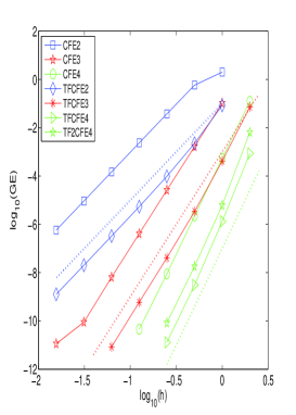
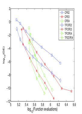
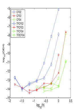
Figure 1. (a) The logarithm of the maximum global error against the logarithm of the stepsize. The dashed lines have slopes four, six and eight. (b) The logarithm of the maximum global error against the logarithm of function evaluations. (c) The logarithm of the maximum global error of Hamiltonian against the logarithm of the stepsize.

Problem 5.2.

Consider the Duffing equation defined by the Hamiltonian :

$$H(p,q)=\frac{1}{2}p^{2}+\frac{1}{2}(\omega^{2}+k^{2})q^{2}-\frac{k^{2}}{2}q^{4}$$

with the initial value $q(0)=0,p(0)=\omega$. The exact solution of this IVP is

$$q(t)=sn(\omega t;k/\omega),\quad p(t)=cn(\omega t;k/\omega)dn(\omega t;k/\omega).$$

where $sn,cn$ and $dn$ are Jacobi elliptic functions. Taking $k=0.07,\omega=5$ and $h=1/5\times 1/2^{i},i=0,1,\ldots,5,$ we integrate this problem over the interval $[0,100]$ by TFCFE$2$, TFCFE$3$, CFE$2$, CFE$3$ and EFCRK$2$ methods. Since the nonlinear term $f$ is polynomial, we can calculate the integrals involved in these methods exactly by Mathematica at the beginning of the computation. Numerical results are shown in Figs. 2.

In Fig. 2(a), one can see that the TF method is more accurate than the non-TF method of the same order under the same stepsize. Both as $2$-stage $4th$-order methods, TFCFE$2$ method is more accurate than EFCRK$2$ method in this problem. Again, it can be observed from Fig. 2(b) that the efficiency of the CFE$r$ method is lower than that of the EF/TF method of the same order. Although the nonlinear integrals are exactly calculated in theory, Fig. 2(c) shows that all of these method only approximately preserve the Hamiltonian. It seems that the rounding error increases as $h\to 0$.

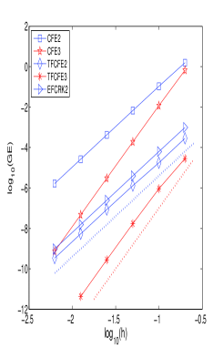
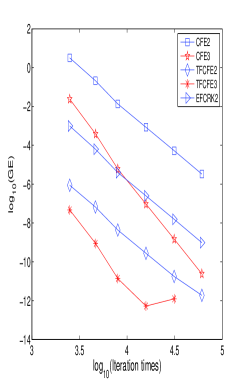
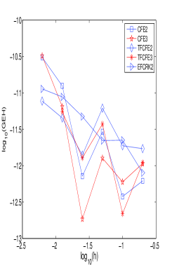
Figure 2. (a) The logarithm of the maximum global error against the logarithm of the stepsize. The dashed lines have slopes four and six. (b) The logarithm of the maximum global error against the logarithm of iteration times. (c) The logarithm of the maximum global error of Hamiltonian against the logarithm of the stepsize.

Problem 5.3.

Consider the Fermi-Pasta-Ulam problem studied by Hairer, et al in [20, 21], which is defined by the Hamiltonian

$$H(p,q)=\frac{1}{2}p^{\intercal}p+\frac{1}{2}q^{\intercal}Mq+U(q),$$

where

$$M=\left(\begin{array}[c]{cc}O_{m\times m}&O_{m\times m}\\ O_{m\times m}&\omega^{2}I_{m\times m}\end{array}\right),$$

$$U(q)=\dfrac{1}{4}\left((q_{1}-q_{m+1})^{4}+\textstyle\sum\limits_{i=1}^{m-1}(q_{i+1}-q_{m+i+1}-q_{i}-q_{m+i})^{4}+(q_{m}+q_{2m})^{4}\right).$$

In this problem, we choose $m=2,q_{1}(0)=1,p_{1}(0)=1,q_{3}(0)=1/\omega,p_{3}(0)=1,$ and zero for the remaining initial values. Setting $\omega=50,h=1/50$ and $\omega=100,h=1/100$, we integrate this problem over the interval $[0,100]$ by CFE2, CFE3, TFCFE2, TFCFE3 and EFCRK2 methods. The nonlinear integrals are calculated exactly by Mathematica at the beginning of the computation. We choose the numerical solution obtained by a high-order method with a sufficiently small stepsize as the ‘reference solution’ in the FPU problem. Numerical results are plotted in Fig. 3.

In Figs. 3(a), 3(c), one can see that the TF methods are more accurate than non-TF ones. Unlike the previous problem, the EFCRK$2$ method wins slightly over TFCFE$2$ method in this case. And Figs. 3(b), 3(d) show that all of these methods display promising EP property , which is especially important in the FPU problem.

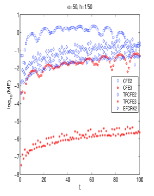
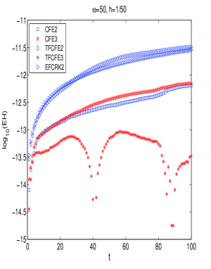
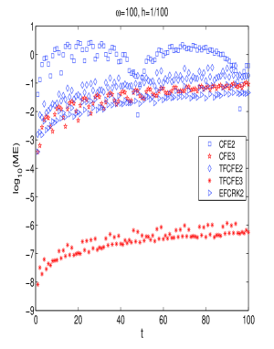
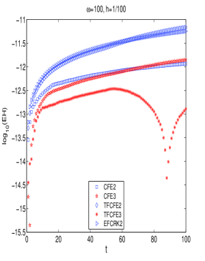
Figure 3. (a) (c) The logarithm of the solution error against time $t$. (b) (d) The logarithm of the Hamiltonian error against time $t$.

Problem 5.4.

Consider the IVP defined by the nonlinear Schrödinger equation

(43) $$\left\{\begin{aligned} &iu_{t}+u_{xx}+2|u|^{2}u=0,\\ &u(x,0)=\varphi(x),\\ \end{aligned}\right.$$

where $u$ is a complex function of $x,t$, and $i$ is the imaginary unit. Taking the periodic boundary condition $u(x_{0},t)=u(x_{0}+L,t)$ and discretizing the spatial derivative $\partial_{xx}$ by the pseudospectral method (see e.g. [13]), this problem is converted into a complex system of ODEs :

$$\left\{\begin{aligned} &i\frac{d}{dt}U+D^{2}U+2|U|^{2}\cdot U=0,\\ &U(0)=(\varphi(x_{0}),\varphi(x_{1}),\ldots,\varphi(x_{d-1}))^{\intercal},\\ \end{aligned}\right.$$

or an equivalent Hamiltonian system:

(44) $$\left\{\begin{aligned} &\frac{d}{dt}P=-D^{2}Q-2(P^{2}+Q^{2})\cdot Q,\\ &\frac{d}{dt}Q=D^{2}P+2(P^{2}+Q^{2})\cdot P,\\ &P(0)=real(U(0)),\quad Q(0)=imag(U(0)),\\ \end{aligned}\right.$$

where the superscript ‘2’ is the entrywise square multiplication operation for vectors, $x_{n}=x_{0}+n\Delta x/d,\ n=0,1,\ldots,d-1,U=(U_{0}(t),U_{1}(t),\ldots,U_{d-1}(t))^{\intercal},P(t)=real(U(t)),Q(t)=imag(U(t))$ and $D=(D_{jk})_{0\leq j,k\leq d-1}$ is the pseudospectral differential matrix defined by:

$$D_{jk}=\left\{\begin{aligned} &\frac{\pi}{L}(-1)^{j+k}cot(\pi\frac{x_{j}-x_{k}}{L}),\ j\neq k,\\ &0,\quad\quad\quad\quad\quad\quad\quad\quad\quad j=k.\\ \end{aligned}\right.$$

The Hamiltonian or the total energy of (44) is

$$H(P,Q)=\frac{1}{2}P^{\intercal}D^{2}P+\frac{1}{2}Q^{\intercal}D^{2}Q+{\frac{1}{2}\sum_{i=0}^{d-1}(P_{i}^{2}+Q_{i}^{2})^{2}.}$$

In [30], the author constructed a periodic bi-soliton solution of (43):

(45) $$u(x,t)=\frac{U(x,t)}{V(x,t)},$$

where

$$U(x,t)=\exp(iM^{2}t)M\cosh^{-1}(M(x-A))-\exp(iN^{2}t)N\cosh^{-1}(N(x+A)),$$

$$V(x,t)=\cosh(J)-\sinh(J)(\tanh(M(x-A))\tanh(N(x+A))$$

$$+\cos((M^{2}-N^{2})t)\cosh^{-1}(M(x-A))\cosh^{-1}(N(x+A))),$$

with

$$J=\tanh^{-1}(\frac{2MN}{M^{2}+N^{2}}).$$

This solution can be viewed approximately as the superposition of two single solitons located at $x=A$ and $x=-A$ respectively. Since it decays exponentially when $x\to\infty$, we can take the periodic boundary condition for sufficiently small $x_{0}$ and large $L$ with little loss of accuracy. Aside from the total energy, it is well known that the semi-discrete NLS (44) has another invariant, the total charge

$$C(P,Q)=\sum_{i=0}^{d-1}(P_{i}^{2}+Q_{i}^{2}).$$

Thus we also calculate the error in the charge(EC):

$$EC=(EC^{0},EC^{1},\ldots)$$

with

$$EC^{n}=|C^{n}-C^{0}|,\quad C^{n}=C(P^{n},Q^{n})$$

where $P^{n}\approx P(t_{n}),Q^{n}\approx Q(t_{n})$ is the numerical solution at the time node $t_{n}$. Taking $x_{0}=-50,L=100,A=10,M=1,N=2^{\frac{1}{2}},d=450,h=0.2,\omega=2,$ we integrate the semi-discrete problem (44) by TFCFE$2$, CFE$2$ and EFGL$2$ methods over the time interval $[0,100]$. The nonlinear integrals are calculated exactly by Mathematica at the beginning of the computation. Numerical results are presented in Fig. 4.

It is noted that the exact solution (45) has two approximate frequency $M^{2}$ and $N^{2}$. By choosing the larger frequency $N^{2}=2$ as the fitting frequency $\omega$, the EF/TF methods still reach higher accuracy than the general-purpose method CFE2, see Fig. 4(a). Among three EF/TF methods, TFCFE2 is the most accurate. Fig. 4(b) shows that three EP methods CFE2, TFCFE2 and EFCRK2 preserve the Hamiltonian (apart from the rounding error). Since EFGL2 is a symplectic method, it preserves the discrete charge, which is a quadratic invariant, see Fig. 4(c). Although TFCFE2 method cannot preserve the discrete charge, its error in the charge is smaller than the charge error of CFE2 and EFCRK2.

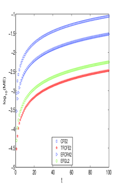
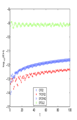
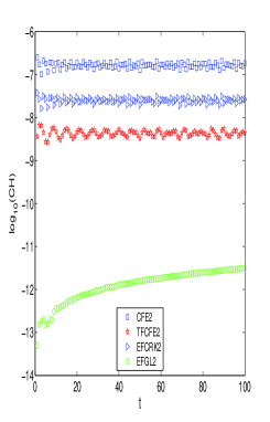
Figure 4. (a) The logarithm of the solution error against time $t$. (b) The logarithm of the Hamiltonian error against time $t$. (c) The logarithm of the charge error against time $t$.

6. Conclusions and discussions

Oscillatory systems constitute an important category of differential equations in numerical simulations. It should be noted that the numerical treatment of oscillatory systems is full of challenges. This paper is mainly concerned with the establishment of high-order functionally-fitted energy-preserving methods for solving oscillatory nonlinear Hamiltonian systems. To this end, we have derived new FF EP methods FFCFE$r$ based on the analysis of continuous finite element methods. The FFCFE$r$ method can be thought of as the continuous-stage Runge–Kutta methods, therefore they can be used conveniently in applications. The geometric properties and algebraic orders of them have been analysed in detail. By equipping FFCFE$r$ with the spaces (7) and (8), we have developed the TF EP methods denoted by TFCFE$r$ and TF2CFE$r$ which are suitable for solving oscillatory Hamiltonian systems with a fixed frequency $\omega$. Evaluating the nonlinear integrals in the EP methods exactly or approximately, we have compared TFCFE$r$ for $r=2,3,4$ and TF2CFE4 with other structure-preserving methods such as EP methods CFE$r$ for $r=2,3,4$, the EP method EFCRK2 and the symplectic method EFGL2. It can be observed from the numerical results that the newly derived TF EP methods show definitely a high accuracy, an excellent invariant-preserving property and a prominent long-term behaviour.

In this paper, our numerical experiments are mainly concerned with the TFCFE$r$ method and oscillatory Hamiltonian systems. However, the FFCFE$r$ method is still symmetric and of order $2r$ for the general autonomous system $y^{\prime}(t)=f(y(t))$. By choosing appropriate function spaces, the FFCFE$r$ method can be applied to solve a much wider class of dynamic systems in applications. For example, the numerical experiment concerning the application of FF Runge–Kutta method to the stiff system has been shown in [29]. Consequently, the FFCFE$r$ method is likely to be a highly flexible method with broad prospects.

References

- [1] P. Betsch, P. Steinmann, Inherently energy conserving time finite element methods for classical mechanics, J. Comput. Phys. 160 (2000) 88-116.
- [2] D. G. Bettis, Numerical integration of products of Fourier and ordinary polynomials, Numer. Math. 14 (1970) 424-434.
- [3] C. L. Bottasso, A new look at finite elements in time : a variational interpretation of Runge–Kutta methods, Appl. Numer. Math. 25 (1997) 355-368.
- [4] L. Brugnano, F. Iavernaro, and D. Trigiante, Hamiltonan Boundary Value Methods (Energy Preserving Discrete Line Integral Methods), J. Numer. Anal. Ind. Appl. Math. 5 (2010) 13-17.
- [5] L. Brugnano, F. Iavernaro, and D. Trigiante, A simple framework for the derivation and analysis of effective one-step methods for ODEs, Appl. Math. Comput. 218 (2012) 8475-8485.
- [6] L. Brugnano, F. Iavernaro, and D. Trigiante, Energy- and quadratic invariants-preserving integrators based upon Gauss-Collocation formulae, SIAM J. Numer. Anal. 50 (2012) 2897-2916.
- [7] M. Calvo, J. M. Franco, J. I. Montijano, and L. Rández, Structure preservation of exponentially fitted Runge–Kutta methods, J. Comput. Appl. Math. 218 (2008) 421-434.
- [8] M. Calvo, J. M. Franco, J. I. Montijano, and L. Rández, On high order symmetric and symplectic trigonometrically fitted Runge–Kutta methods with an even number of stages, BIT Numer. Math. 50 (2010) 3-21.
- [9] M. Calvo, J. M. Franco, J. I. Montijano, and L. Rández, Symmetric and symplectic exponentially fitted Runge–Kutta methods of high order, Comput. Phys. Comm. 181 (2010) 2044-2056.
- [10] E. Celledoni, R. I. Mclachlan, D. I. Mclaren, B. Owren, G. R. W. Quispel, and W. M. Wright, Energy-preserving Runge–Kutta methods, ESIAM. Math. Model. Numer. Anal. 43 (2009) 645-649.
- [11] E. Celledoni, R. I. Mclachlan, B. Owren, and G. R. W. Quispel, Energy-preserving integrators and the structure of B-series, Found. Comput. Math. 10 (2010) 673-693.
- [12] E. Celledoni, V. Grimm, R. I. Mclachlan, D. I. Mclaren, D. O’Neale, B. Owren, and G. R. W. Quispel, Preserving energy resp. dissipation in numerical PDEs using the ‘Average Vector Field’ method, J. Comput. Phys. 231 (2012) 6770-6789.
- [13] J. B. Chen, M. Z. Qin, Multisymplectic Fourier pseudospectral method for the nonlinear Schrödinger equation, Electron. Trans. Numer. Anal. 12 (2001) 193-204.
- [14] J. P. Coleman, P-stability and exponential-fitting methods for , IMA J. Numer. Anal. 16 (1996) 179-199.
- [15] J. M. Franco, Exponentially fitted symplectic integrators of RKN type for solving oscillatory problems, Comput. Phys. Comm. 177 (2007) 479-492.
- [16] D. A. French, J. W. Schaeffer, Continuous finite element methods which preserve energy properties for nonlinear problems, Appl. Math. Comput. 39 (1990) 271-295.
- [17] W. Gautschi, Numerical integration of ordinary differential equations based on trigonometric polynomials, Numer. Math. 3 (1961) 381-397.
- [18] O. Gonzalez, Time Integration and Discrete Hamiltonian Systems, J. Nonlinear Sci. 6 (1996) 449-467.
- [19] E. Hairer, Variable time step integration with symplectic methods, Appl. Numer. Math. 25 (1997) 219-227.
- [20] E. Hairer, C. Lubich, Long-time energy conservation of numerical methods for oscillatory differential equations. SIAM J. Numer. Anal. 38 (2000) 414-441.
- [21] E. Hairer, C. Lubich, G. Wanner, Geometric Numerical Integration, 2nd edn. Springer, Berlin (2006).
- [22] E. Hairer, Energy-preserving variant of collocation methods, J. Numer. Anal. Ind. Appl. Math. 5 (2010) 73-84.
- [23] N. S. Huang, R. B. Sidge, N. H. Cong, On functionally fitted Runge–Kutta methods, BIT Numer. Math. 46 (2006) 861-874.
- [24] B. L. Hulme, One-step piecewise polynomial Galerkin methods for initial value problems, Math. Comp. 26 (1972) 415-426.
- [25] L.Gr. Ixaru, G. Vanden Bergehe (eds.), Exponential Fitting, Kluwer Academic Publishers, Dordrecht,2004.
- [26] R. I. Mclachlan, G. R. W Quispel, and N. Robidoux, Geometric Integration Using Dicrete Gradients, Philos. Trans. R. Soc. A 357 (1999) 1021-1046.
- [27] Y. Miyatake, An energy-preserving exponentially-fitted continuous stage Runge–Kutta method for Hamiltonian systems, BIT Numer. Math. 54 (2014) 777-799.
- [28] Y. Miyatake, A derivation of energy-preserving exponentially-fitted integrators for Poisson systems, Comput. Phys. Comm. 187 (2015) 156-161.
- [29] K. Ozawa, A functionally fitting Runge–Kutta method with variable coefficients, Jpn. J. Ind. Appl. Math. 18 (2001) 107-130.
- [30] D. H. Peregrine, Water waves, nonlinear Schrödinger equations and their solutions, J. Austral. Math. Soc. Ser B 25 (1983) 16-43.
- [31] L. R. Petzold, L. O. Jay, Y. Jeng, Numerical solution of highly oscillatory ordinary differential equations, Acta Numerica 6 (1997) 437-483.
- [32] J. C. Simos, Assessment of energy-momentum and symplectic schemes for stiff dynamical systems, American Sociery for Mechanical Engineers, ASME Winter Annual meeting, New Orleans, Louisiana, 1993.
- [33] T. E. Simos, An exponentially-fitted Rung–Kutta method for the numerical integration of initial-value problems with periodic or oscillating solutions, Comput. Phys. Comm. 115 (1998) 1-8.
- [34] T. E. Simos, Does variable step size ruin a symplectic integrator? Physica D: Nonlinear Phenomena 60 (1992) 311-313.
- [35] W. Tang, Y. Sun, Time finite element methods : A unified framework for the numerical discretizations of ODEs, Appl. Math. Comput. 219 (2012) 2158-2179.
- [36] G. Vanden Berghe, Exponentially-fitted Runge–Kutta methods of collocation type : fixed or variable knots?, J. Comput. Appl. Math. 159 (2003) 217-239.
- [37] H. Van de Vyver, A fourth order symplectic exponentially fitted integrator, Comput. Phys. Comm. 176 (2006) 255-262.
- [38] B. Wang, A. Iserles, X. Wu, Arbitrary order trigonometric Fourier collocation methods for multi-frequency oscillatory systems, Found. Comput. Math. (2014): DOI 10.1007/s10208-014-9241-9.
- [39] X. Wu, B. Wang, A new high precision energy-preserving integrator for system of second-order differential equations, Physics Letters A 376 (2012) 1185-1190.
- [40] X. Wu, B. Wang, J. Xia, Explicit symplectic multidimensional exponential fitting modified Runge–Kutta–Nyström methods, BIT Numer. Math. 52 (2012) 773-791.
- [41] H. Yang, X. Wu, X. You, Y. Fang, Extended RKN-type methods for numerical integration of perturbed oscillators , Comput. Phys. Comm. 180 (2009) 1777-1794.