A Plug-and-Play Priors Framework for Hyperspectral Unmixing

Abstract

Spectral unmixing is a widely used technique in hyperspectral image processing and analysis. It aims to separate mixed pixels into the component materials and their corresponding abundances. Early solutions to spectral unmixing are performed independently on each pixel. Nowadays, investigating proper priors into the unmixing problem has been popular as it can significantly enhance the unmixing performance. However, it is non-trivial to handcraft a powerful regularizer, and complex regularizers may introduce extra difficulties in solving optimization problems in which they are involved. To address this issue, we present a plug-and-play (PnP) priors framework for hyperspectral unmixing. More specifically, we use the alternating direction method of multipliers (ADMM) to decompose the optimization problem into two iterative subproblems. One is a regular optimization problem depending on the forward model, and the other is a proximity operator related to the prior model and can be regarded as an image denoising problem. Our framework is flexible and extendable which allows a wide range of denoisers to replace prior models and avoids handcrafting regularizers. Experiments conducted on both synthetic data and real airborne data illustrate the superiority of the proposed strategy compared with other state-of-the-art hyperspectral unmixing methods.

I Introduction

Hyperspectral imaging is a continuously growing field and has received increasing interest in the past few years. In contrast to traditional RGB and multispectral images providing a limited number of spectral channels, hyperspectral images capture hundreds of spectral bands, and this rich spectral information facilitates the analysis of elements in the scenes [2, 3]. However, due to factors such as the low spatial resolution and the presence of multiple scattering, an observed pixel usually contains a mixture of several materials. The presence of mixed pixels restricts the interpretability of the data and has an adverse impact on the accuracy of various tasks, such as image classification [4] and target detection[5]. Spectral unmixing is thus playing an important role in hyperspectral image processing. This technique aims at decomposing a mixed pixel spectrum into a set of pure spectral signatures called endmembers, and their corresponding fractional abundances [6, 7].

There exist many hyperspectral unmixing methods, and most of them are based on the linear mixing model (LMM) due to its simplicity and physical interpretability [8, 9, 10]. The LMM assumes that an observed pixel spectrum is a linear combination of a set of endmembers weighted by their associated fractional abundances [11, 12]. Though the LMM has practical advantages, there are many situations where the incoming light may undergo complex interactions and multiple photon reflections introduce nonlinear effects on the mixed spectra [13]. The mixing model is then advantageously formulated as a nonlinear one. The work [12] proposes an augmented LMM to address the spectral variability issue. In our work, we focus on designing a flexible strategy to exploit proper priors to the unmixing task. Without loss of the generality, we discuss our method based on the LMM.

The spectral signatures of endmembers can be extracted from hyperspectral data or selected from a library. Under the assumption that the endmembers are known in advance, the unmixing task is committed to estimating the fractional abundances [14, 13, 15, 16]. Early unmixing methods, such as the fully constrained least square method (FCLS) [14] and the non-negative constrained least square error method (NCLS) [14], are pixel-by-pixel algorithms and ignore the prior information existing in hyperspectral images. Nevertheless, natural hyperspectral images usually contain various inherent correlations in both spatial and spectral domains. Properly using this prior information can effectively enhance the unmixing performance.

A significant amount of regularized unmixing algorithms have been proposed in recent years. One such regularizer is the total-variation (TV) regularizer. In [17], a TV regularizer is imposed on the reconstructed image to incorporate the spatial and spectral information via pixel links in the unmixing problem. The spatial smoothness of hyperspectral images can also be employed to abundance maps. The SUnSAL-TV method [18] introduces a TV regularizer to enhance the spatial consistency of estimated abundances. However, classical TV regularizers are restrictive due to their assumption in local spatial correlations, i.e., a pixel is similar to its neighbors [19, 20]. The non-local regularizers take non-local spatial information into consideration to fully exploit similar patterns and structures across the image [21, 22, 23]. Graph-based regularizers capture the features in arbitrary neighborhood [22]. The works [24, 25] use superpixel methods to generate the spatial groups and exract local pixels with homogenous spectra. In [26], $\ell_{1}$-norm is used to constrain the spatial and spectral domains to impose sparsity on the solution. In [27], subspace unmixing with low-rank attribute embedding (SULoRA) is proposed to jointly estimate subspace projections and abundance maps. It solves a constrained optimization problem with subspace and abundance regularizers. Therefore, properly introducing constraints and designing ingenious regularizers play an important role in improving the unmixing performance. However, it is a non-trivial task to handcraft an effective regularizer, and complex regularizers may increase the difficulty of solving associated optimization problems. Inspired by the successful applications of deep learning, convolutional neural networks (CNNs) have been introduced to learn spatial and spectral priors to conduct hyperspectral unmixing. The work [28] utilizes a 2D CNN framework to make use of the spatial and spectral information of hyperspectral images. In [29] and [30], 3D convolution based models are proposed to integrate spatial and spectral priors. However, these CNN based methods only focus on local areas and fail to capture nonlocal features of hyperspectral images.

Recently, benefiting from variable splitting techniques, many plug-and-play priors (PnP) methods have received great success in many hyperspectral image processing tasks (regarded as linear inverse problems), such as denoising [31, 32], deconvolution [33, 34] and pansharpening [35, 36]. Instead of using handcrafted regularizers, these PnP priors based approaches plug denoising methods as a module to replace the proximity operator in the iterative optimization procedure [37, 38]. The alternating direction method of multipliers (ADMM) [39] is widely used as the variable splitting technique in these image restoration approaches, for its well-known convergence property [36, 37]. In these methods, the spatial and spectral characteristics existing in 3D domain can be captured with denoisers. Various denoisers, which are regarded as black-boxes, can be flexibly injected. Another popular strategy is directly employing deep neural networks to solve linear inverse problems in an end-to-end way, an overview of recent state-of-the-art deep learning methods can be found in [40].

In this paper, we propose a novel framework based on ADMM to introduce prior information of abundance maps and hyperspectral images in the unmixing task. Without handcrafting regularizers, we incorporate different denoisers into this framework to capture various spatial and spectral correlations. Also, adopting denoisers significantly improves the robustness of the proposed unmixing method to noise interruption. The usage of various denoisers demonstrates the flexibility and extendability of our framework. We summarize our contributions as follows:

• In our work, we extend the PnP priors framework to propose a robust hyperspectral unmixing method. Our scheme is based on ADMM algorithm, which decomposes the associated optimization problem into two subproblems. Specifically, one of the subproblem is a proximity operator related to the prior model and can be replaced by a denoising operator.

• A variety of denoisers are plugged into the proposed unmixing framework, including linear and non-linear, band-wise and 3D, traditional and deep learning based. These denoising operators allows us to exploit various priors of images and bypass the difficulty in designing regularizers.

• The proposed framework is designed to incorporate denoisers with two strategies. One exploits the spatial and spectral prior information from reconstructed hyperspectral images. The other one captures the spectral and spatial correlations directly from fractional abundance maps and alleviates the computational burden.

The paper is organized as follows. In Section II, the outline of the PnP priors framework for linear inverse problem is presented. Section III presents the proposed a unmixing method based on PnP priors with a variety of denoisers. In Section IV, both synthetic and real data experiments are conducted and analyzed. Section V concludes this paper.

II Plug-and-play Priors framework

In this section, we outline the PnP priors framework for the linear inverse problem. Let $\mathbf{d}$ be the observed data, $\mathbf{x}$ is the hidden parameters to be estimated. A general description of the linear inverse problem is

$$\mathbf{d}=\mathcal{S}(\mathbf{x})+\mathbf{n},$$ (1)

where $\mathcal{S}(\cdot)$ presents the linear forward model, $\mathbf{n}$ is an additive independent and identically distributed (i.i.d.) Gaussian noise. We can estimate $\mathbf{x}$ by seeking the minimum of the following objective function:

$$\mathbf{\hat{x}}=\arg\min_{\mathbf{x}}\frac{1}{2}\|\mathbf{d}-\mathcal{S}(\mathbf{x})\|_{2}^{2}+\lambda J(\mathbf{x}),$$ (2)

where $J(\mathbf{x})$ presents a regularizer encoding the prior information to enforce the desired property of the solution, and $\lambda$ is a positive penalty parameter to control the impact of $J(\mathbf{x})$.

Various algorithms have been proposed to solve this problem, the proposed framework is based on ADMM to solve the optimization problem (2) owing to its good convergence property. We introduce an auxiliary variable $\mathbf{v}$ and the problem (2) can be rewritten as:

$$\begin{split}\mathbf{\hat{x}}=\arg\min_{\mathbf{x}}&\frac{1}{2}\|\mathbf{d}-\mathcal{S}(\mathbf{x})\|_{2}^{2}+\lambda J(\mathbf{v}),\\ &\text{s.t.}~{}~{}\mathbf{v}=\mathbf{x}.\end{split}$$ (3)

The associated augmented Lagrangian function is given by

$$\mathbf{\hat{x}}=\arg\min_{\mathbf{x}}\frac{1}{2}\|\mathbf{d}-\mathcal{S}(\mathbf{x})\|_{2}^{2}+\lambda J(\mathbf{v})+\frac{\rho}{2}\|\mathbf{x}-\mathbf{v}+\mathbf{u}\|_{2}^{2},$$ (4)

where $\mathbf{u}$ is the scaled dual variable, and $\rho$ is the penalty parameter. Then the optimization problem (4) can be solved by repeating the following steps:

$$\tilde{\mathbf{x}}\leftarrow\mathbf{\hat{v}}-\mathbf{u};$$ (5)

$$\mathbf{\hat{x}}\leftarrow\arg\min_{\mathbf{x}}\frac{1}{2}\|\mathbf{d}-\mathcal{S}(\mathbf{x})\|_{2}^{2}+\frac{\rho}{2}\|\mathbf{\tilde{x}}-\mathbf{x}\|_{2}^{2};$$ (6)

$$\tilde{\mathbf{v}}\leftarrow\mathbf{\hat{x}}+\mathbf{u};$$ (7)

$$\mathbf{\hat{v}}\leftarrow\arg\min_{\mathbf{v}}\lambda J(\mathbf{v})+\frac{\rho}{2}\|\mathbf{\tilde{v}}-\mathbf{v}\|_{2}^{2};$$ (8)

$$\mathbf{u}\leftarrow\mathbf{u}+\mathbf{\hat{x}}-\mathbf{\hat{v}}.$$ (9)

The steps include two key operators. The step (6) is a linear inverse operator, and the step (8) is the proximity operator that can be considered as a denoising problem. From a Bayesian viewpoint, the problem in step (8) can be regarded as a denoising problem. We can replace this step with a variety of denoisers rather than solving it with an explicit form. This strategy avoids handcrafting the regularizer $J(\mathbf{v})$ and exploits priors of the hidden parameters by using denoisers.

III Application to spectral unmixing

III-A Problem Formulation

We denote a hyperspectral image as $\mathbf{Y}_{\text{3D}}\in\mathbb{R}^{L\times M\times K}$, where $L$, $M$ and $K$ are the numbers of spectral bands, rows and columns of the image. For ease of mathematical formulation, the columns of image $\mathbf{Y}_{\text{3D}}$ are stacked to form $\mathbf{Y}\in\mathbb{R}^{L\times N}$ with $N=M\times K$ representing the number of hyperspectral pixels. The LMM for a hyperspectral image is based on the assumption that a pixel of hyperspectral data is a linear mixture of endmembers. We express it as:

$$\mathbf{Y}=\mathbf{MA}+\mathbf{N},$$ (10)

where $\mathbf{Y}=[\mathbf{y}_{1},\cdots,\mathbf{y}_{N}]\in\mathbb{R}^{L\times N}$ and $\mathbf{y}_{i}$ is the signature vector corresponding to the $i$-th pixel in the hyperspectral image. $\mathbf{M}\in\mathbb{R}^{L\times P}$ is the endmember matrix containing $P$ spectral signatures. $\mathbf{A}=[\mathbf{a}_{1},\cdots,\mathbf{a}_{N}]\in\mathbb{R}^{P\times N}$ is the abundance matrix and $\mathbf{a}_{i}$ denotes the corresponding fractional abundances of the $i$-th hyperspectral pixel. $\mathbf{N}=[\mathbf{n}_{1},\cdots,\mathbf{n}_{N}]\in\mathbb{R}^{L\times N}$ represents the i.i.d. Gaussian noise. As the abundances represent the relative amount of each endmember, they need to be non-negative (abundance nonnegativity constraint, ANC). Furthermore, the entire spectra are decomposed into endmember contributions, and thus the abundance fractions should satisfy the abundance sum-to-one constraint (ASC). The ANC and ASC can be defined as follows:

$${a}_{ij}\geq 0,\quad\forall i,j$$ (11)

$$\sum_{i=1}^{P}a_{ij}=1,\quad\forall j.$$ (12)

With a known endmember matrix $\mathbf{M}$, the estimation of abundances can be obtained by solving the following optimization problem,

$$\begin{split}&\min_{\mathbf{A}}\frac{1}{2}\|\mathbf{Y}-\mathbf{MA}\|_{\text{F}}^{2},\\ \text{s.t.}~{}~{}{a}_{ij}&\geq 0,\quad\forall i,j,\quad\sum_{i=1}^{P}{a}_{ij}=1,\quad\forall j,\end{split}$$ (13)

where $\|\cdot\|_{\text{F}}$ is the Frobenius norm of the matrix. Compared to performing unmixing on each individual pixel, incorporating proper regularizers is effective to enhance the unmixing performance. The regularization term can be imposed on the reconstructed image or directly on the abundances. In our work, we aim to exploit priors of reconstructed images and abundance maps respectively according to the different choices of the pattern switch matrix $\mathbf{H}$, and the optimization problem in (3) can be formulated as:

$$\begin{split}&\min_{\mathbf{A}}\frac{1}{2}\|\mathbf{Y}-\mathbf{MA}\|_{\text{F}}^{2}+\lambda\Phi(\mathbf{HA})\\ \text{s.t.}~{}~{}&{a}_{ij}\geq 0,\quad\forall i,j,\quad\sum_{i=1}^{P}a_{ij}=1,\quad\forall j.\end{split}$$ (14)

The squared-error term $\|\mathbf{Y}-\mathbf{MA}\|_{\text{F}}^{2}$ is the data fidelity term while the second term $\Phi(\mathbf{HA})$ is a regularization term, which is defined to further promote desired property of the results. The proposed framework is suggested to be conducted using two forms:

• Pro-H: $\mathbf{H}=\mathbf{M}$, $\Phi(\mathbf{HA})$ is used to penalize on reconstructed images;

• Pro-A: $\mathbf{H}=\mathbf{I}$ where $\mathbf{I}$ is identity matrix, $\Phi(\mathbf{HA})$ is used to penalize on abundance maps directly.

$\lambda$ is a positive parameter trading off the data fidelity term and the regularization term.

III-B Proposed Plug-and-Play Framework for Hyperspectral Unmixing

Designing a powerful regularizer is a non-trivial task, and complex regularizers usually make the optimization problem more complicated to solve. In our work, we aim to use the variable splitting strategy to create a flexible and extendable PnP priors framework to tackle the unmixing problem. It allows various image denoisers (linear or non-linear, band-wise or 3D, traditional or deep learning based) to replace the design of regularizers. More specially, the optimization problem (LABEL:eq.lms_model_22) is decoupled into two sub-problems: a quadratic programming (QP) sub-problem with linear constraints and an image denoising sub-problem. These sub-problems are then solved iteratively to estimate the final abundance.

ADMM is adopted to decouple the data fidelity term and the regularization term in (LABEL:eq.lms_model_22). By introducing an auxiliary variable $\mathbf{Z}$, problem (LABEL:eq.lms_model_22) is equivalent to:

$$\begin{split}&\min_{\mathbf{A},\mathbf{Z}}\frac{1}{2}\|\mathbf{Y}-\mathbf{MA}\|_{\text{F}}^{2}+\lambda\Phi(\mathbf{Z})\\ &\text{s.t.}~{}~{}\mathbf{Z}=\mathbf{HA}\\ &~{}~{}~{}~{}~{}{a}_{ij}\geq 0,\quad\forall i,j,\quad\sum_{i=1}^{P}a_{ij}=1,\quad\forall j{\color[rgb]{0,0,0}.}\end{split}$$ (15)

The corresponding augmented Lagrangian function with the scaled dual variable $\mathbf{U}$ is

$$\mathcal{L}_{\rho}({\bf A,Z})= \arg\mathop{\min}_{{\bf A,\bf Z}}\,\frac{1}{2}\|\mathbf{Y}-\mathbf{MA}\|_{\text{F}}^{2}+\lambda\Phi({\bf Z})$$ (16)

$$+\frac{\rho}{2}\|{\bf HA-Z+U}\|_{\text{F}}^{2}$$

$$\text{s.t.}~{}~{}{a}_{ij} \geq 0,\quad\forall i,j,\quad\sum_{i=1}^{P}a_{ij}=1,\quad\forall j$$

where $\rho$ is a positive penalty parameter. According to the PnP priors framework for the linear inverse problem, (16) can be solved by repeating the following steps until convergence:

$${\bf A}_{k+1}= \arg\mathop{\min}_{{\bf A}}\,\frac{1}{2}\|{\bf Y}-{\bf M}{\bf A}_{k}\|_{\text{F}}+\frac{\rho_{k}}{2}\|{\bf HA}_{k}-{\bf\tilde{\bf X}}_{k}\|_{\text{F}}$$ (17)

s.t. $$~{}~{}{a}_{ij}\geq 0,\quad\forall i,j,\quad\sum_{i=1}^{P}a_{ij}=1,\quad\forall j.$$

$${\bf Z}_{k+1}=\arg\mathop{\min}_{{\bf Z}}\,\lambda\Phi({\bf Z})+\frac{\rho_{k}}{2}\|{\tilde{\bf Z}}_{k}-{\bf Z}\|_{\text{F}}^{2}$$ (18)

$${\bf U}_{k+1}={\bf U}_{k}+{\bf HA}_{k+1}-{\bf Z}_{k+1}$$ (19)

$${\rho}_{k+1}={\alpha\rho}_{k}$$ (20)

where ${\tilde{\bf X}}_{k}={\bf Z}_{k}-{\bf U}_{k}$ and ${\tilde{\bf Z}}_{k}={\bf HA}_{k+1}+{\bf U}_{k}$. The objective function (LABEL:eq.object_equ) is thus decoupled into two subproblems (17) and (18). We solve the QP problem (17) pixel by pixel. For a hyperspectral pixel ${\bf y}_{i}$, this problem can be reformulated as

$${\bf a}_{k+1,i} =\arg\mathop{\min}_{{\bf a}_{i}}\,\frac{1}{2}\|{\bf y}_{i}-{\bf M}{\bf a}_{i}\|^{2}+\frac{\rho_{k}}{2}\|{\bf Ha}_{i}-{\bf\tilde{\bf x}}_{k,i}\|^{2}$$ (21)

$$=\arg\mathop{\min}_{{\bf a}_{i}}\frac{1}{2}{{\bf a}_{i}^{\top}}{\bf Q}{\bf a}_{i}+{\bf f}^{\top}{\bf a}_{i}$$

$$\text{s.t.}~{}~{}{a}_{ij}\geq 0,\quad\forall i,j,\quad\sum_{i=1}^{P}a_{ij}=1,\quad\forall j{\color[rgb]{0,0,0},}$$

where $\mathbf{Q}=\mathbf{M}^{\top}\mathbf{M}+{\rho_{k}}\mathbf{H}^{\top}\mathbf{H}$ and $\mathbf{f}=-(\mathbf{M}^{\top}\mathbf{y}_{i}+{\rho_{k}}\mathbf{H}^{\top}\tilde{\mathbf{x}}_{k,i})$. The QP problem in (21) is a standard FCLS problem, which can be solved by a generic QP solver. The second step involving regularizer in (18) can be rewritten as:

$${\bf Z}_{k+1}=\arg\mathop{\min}_{{\bf Z}}\,\frac{1}{2(\sqrt{{\lambda}/{\rho_{k}}})^{2}}\|{\tilde{\bf Z}}_{k}-{\bf Z}\|_{\text{F}}^{2}+\Phi({\bf Z}).$$ (22)

Based on Bayesian theory, the problem in (22) can be regarded as an image denoising problem to remove additive Gaussian noise with a standard deviation $\sigma_{n}=\sqrt{{\lambda}/{\rho_{k}}}$. In form Pro-H, this step aims to obtain a clean reconstructed hyperspectral image ${\bf Z}_{k+1}$ from the noisy observations $\tilde{\bf Z}_{k}$ with a noise level $\sqrt{{\lambda}/{\rho_{k}}}$ . In form Pro-A, this step becomes an abundance maps denoising operator. It is worth noting that, compared to Pro-H, Pro-A alleviates the computational burden since abundance maps always have smaller volumes than reconstructed hyperspectral images.

Instead of solving the step (18) in an explicit form, we replace it with various denoisers. In other words, the denoiser extracting prior information is plugged into the iterative algorithm to solve the step (18), which is so-called PnP priors. The denoising operator is actually performed in the 3D domain, we rewrite (22) as follows:

$${\bf Z}_{k+1}=\mathcal{T}^{-1}(\textit{Denoiser}({\mathcal{T}(\tilde{\bf Z}}_{k}),\sqrt{{\lambda}/{\rho_{k}}})),$$ (23)

where $\mathcal{T}(\cdot)$ is an operator to reshape a 2D matrix to a 3D data cube and $\mathcal{T}^{-1}(\cdot)$ is the opposite operator. In this way, the input of the denoiser is a 3D image cube and the denoiser can jointly capture the spatial and spectral information.

In order to force the constraint $\mathbf{Z}=\mathbf{HA}$ to be ideal and affect the noise level $\sqrt{{\lambda}/{\rho}}$ to make the denosier more conservative with iterations, we increase the penalty parameter $\rho$ with scaling factor $\alpha$ during the iterations in (20). The procedure of our PnP priors framework is summarized in Algorithm 1.

Data: A hyperspectral image $\bf Y$, endmembers $\bf M$, the number of hyperspectral pixels $N$, the regularization parameter $\lambda$, the penalty factor $\rho$, the number of iterations $K$, the scaling factor $\alpha$, the pattern switch matrix $\bf H$.

Result: Fractional abundance $\bf A$.

1 Initialize ${\bf A}$ randomly, initialize the auxiliary variable ${\bf Z}_{0}={\bf MA}_{0}$,

2 scaled dual variable ${\bf U}_{0}=\bf 0$, $k=0$;

3 while Stopping criterias are not met and $k\leq K$ do

4       ${\tilde{\bf X}}_{k}={\bf Z}_{k}-{\bf U}_{k}$;

5       for $i=1$ to $N$ do

6             Calculate ${\bf a}_{k+1,i}$ in (21) by using a generic QP solver;

7            

8       end for

9       ${\tilde{\bf Z}}_{k}={\bf HA}_{k+1}+{\bf U}_{k}$;

10       ${\bf Z}_{k+1}=\mathcal{T}^{-1}(\textit{Denoiser}(\mathcal{T}({\tilde{\bf Z}}_{k}),\sqrt{{\lambda}/{\rho_{k}}}))$;

11       ${\bf U}_{k+1}={\bf U}_{k}+{\bf HA}_{k+1}-{\bf Z}_{k+1}$;

12       $\rho_{k+1}=\alpha\rho_{k}$;

13       $k=k+1$;

14      

15 end while

Algorithm 1 Plug-and-play priors framework for hyperspectral unmixing.

III-C Denoisers Plugged into Plug-and-Play Priors Framework

Benefiting from the generalization ability of the proposed PnP priors framework for hyperspectral unmixing, different denoising algorithms can be plugged into it as prior models. Our framework is thus opening a huge opportunity to adopt a wide variety of prior information. In our work, we use popular and effective denoising operators in the PnP framework iterations, including linear or non-linear, band-wise or 3D, and traditional or deep learning based denoisers. Specifically, this work investigates the following denoisers:

• Non-local means denoising (NLM) [41]: NLM is a filter based image deniosing algorithm. This denoiser is linear and based on a non-local averaging of similar pixels in the image. Our proposed unmixing methods plugging NLM are named as Pro-H-NLM and Pro-A-NLM, respectively.

• Block-matching and 3D filtering (BM3D) [42]: BM3D is a non-linear denoiser proposed to use collaborative filter to reduce the noise of grouped image blocks. We denote our proposed unmixing methods using the BM3D as Pro-H-BM3D and Pro-A-BM3D, respectively.

• BM4D [43]: BM4D is a 3D cube based denoising algorithm extended from BM3D, which has been successfully applied to volumetric images. It can make full use of the spectral information as well as spatial correlation of volumetric data. We denote our proposed unmixing methods using BM4D denoiser as Pro-H-BM4D and Pro-A-BM4D, respectively.

• A total variation regularized low-rank tensor decomposition denoising model (LRTDTV) [44]: LRTDTV is a hyperspectral denoising method using an anisotropic spatial-spectral total variation regularization to characterize the smooth priors from spatial and spectral domains. The tensor Tucker decomposition is used to describe the global correlation in all bands. We use this method to denoise reconstructed hyperspectral images and name the corresponding unmixing method as Pro-H-LRTDTV.

• Denoising convolutional neural network (DnCNN) [45]: DnCNN is a deep learning based denoiser using a convolutional neural network. We use this method to denoise the abundance maps and this strategy is named as Pro-A-DnCNN. Considering the similar text features between natural images and abundance maps, we directly use this denoising network with default network parameters trained by natural image datasets, which is online available. Besides, a transfer learning strategy is considered, we generate the ground truth of abundance maps to fine tune models trained by natural images.

IV Experiments

In this section, we illustrate the performance of the proposed PnP priors based unmixing methods. Experiments on both synthetic data and real airborne images are conducted. Several state-of-the-art methods, FCLS [14], SUnSAL-TV [18], CsUnL0 [46] and SCHU [25] are implemented to compare with the proposed unmixing methods. FCLS is a conventional unmixing method and aims to minimize the least square error with the ANC and ASC. SUnSAL-TV is a sparse unmixing method with a TV-norm regularizer and solved using ADMM. CsUnL0 is a collaborative sparse unmixing approach using $\ell_{0}$-norm. SCHU is a graph-based unmixing method via the superpixel, which divides pixels of an image into local clusters that exhibit similar features.

The performance of abundance estimation is evaluated using the root-mean-square-error (RMSE) given by

$$\text{RMSE}=\sqrt{\frac{1}{NP}\sum_{i=1}^{N}\|\mathbf{a}_{i}-\hat{\mathbf{a}}_{i}\|^{2}},$$ (24)

where $\mathbf{a}_{i}$ and $\hat{\mathbf{a}}_{i}$ denote the true and estimated abundance vectors of the $i$-th pixel, respectively. Further, we use the peak signal-to-noise ratio (PSNR) to evaluate the image denoising quality, which is defined by:

$$\text{PSNR}=10\times\log_{10}\left(\frac{\text{MAX}^{2}}{\text{MSE}}\right),$$ (25)

we use the reconstructed hyperspectral image defined by $\mathbf{\hat{Y}}=\mathbf{M}\hat{\mathbf{A}}$ and the ground truth $\mathbf{\tilde{Y}}=\mathbf{M}\mathbf{A}$ to calculate PSNR. MAX is the maximum pixel value of $\mathbf{\hat{Y}}$, and MSE is the mean square error between $\mathbf{\hat{Y}}$ and $\mathbf{\tilde{Y}}$, which is defined by:

$$\text{MSE}=\frac{1}{MK}\sum_{i=1}^{M}\sum_{j=1}^{K}\|\mathbf{\hat{Y}}(i,j)-\mathbf{\tilde{Y}}(i,j)\|^{2},$$ (26)

where $M$ and $K$ are the numbers of rows and columns of the image.

IV-A Experiments with Synthetic Dataset

In these experiments, we generate a synthetic dataset to evaluate the unmixing methods in both quantitative and qualitative manners.

IV-A1 Data Description

Synthetic data are generated using the U.S. Geological Survey (USGS) spectral library. The USGS spectral library consists of 500 mineral materials, which can be download at the website. The hyperspectral image consists of 224 contiguous bands. We use $4$ spectral signatures ($P=4$) which are randomly selected from the USGS spectral library to build the endmember matrix $\mathbf{M}$. This data is generated following the method of Hyperspectral Imagery Synthesis tools, and we use Gaussian Fields to form the abundance matrix $\mathbf{A}$. There are both mixed and pure pixels in the dataset, and our dataset is also built with spatial correlation between neighboring pixels. The abundances are restricted to satisfy the ANC and ASC. The spatial resolution is set to $256\times 256$, and all spectral bands are used in our synthetic data. In order to verify the denoising ability of the proposed method, we add zero-mean Gaussian noise to this data, with the SNR setting to 5 dB, 10 dB, 20 dB and 30 dB, respectively. The ground-truth reference of synthetic data is shown in the first column of Figure 2.

We generate 400 simulated abundance maps with the spatial resolution $256\times 256$ to train the models of DnCNN. The learning rate is set to one hundredth of the original one, and the batch size is set to 16. We fine tune the network with different SNRs, namely, 10 dB, 15 dB, 20 dB, 25 dB, 30 dB, 35 dB, 40 dB, 45 dB, 50 dB, 55 dB and 60 dB.

IV-A2 Unmixing Results and Discussion

The setting values of $\rho$ and $\lambda$ used in experiments of this dataset are presented in Table I. We set $\alpha=1$ for experiments of denoising hyperspectral images (Pro-H), and $\alpha=1.1$ for experiments of denoising abundance maps (Pro-A). Figure 1 illustrates how parameters $\rho$ and $\lambda$ affect the performance of Pro-H-NLM using the synthetic data with SNR=20 dB. We can see that within a reasonable range of parameter values our method obtains a satisfactory unmixing result, and a good selection of $\rho$ and $\lambda$ makes the method easily find a solution near the optimal result. It is noted that $\lambda$ controls the impact of regularization term and has an effect on the unmixing results. $\rho$ is a penalty parameter in the augmented Lagrangian function and only influence the convergence speed.

TABLE I: RMSE and PSNR Comparison of Synthetic Dataset.

	5dB		10dB		20dB		30dB
	RMSE	PSNR	RMSE	PSNR	RMSE	PSNR	RMSE	PSNR
FCLS	0.0897	31.194	0.0581	35.435	0.0200	44.964	0.0064	55.647
SUnSAL-TV	0.0802	31.278	0.0492	35.698	0.0199	45.892	0.0064	55.774
	($\lambda_{\text{TV}}=1\times 10^{-2}$)		($\lambda_{\text{TV}}=5\times 10^{-3}$)		($\lambda_{\text{TV}}=5\times 10^{-3}$)		($\lambda_{\text{TV}}=5\times 10^{-3}$)
CsUnL0	0.1078	30.819	0.0695	35.199	0.0242	44.734	0.0077	54.709
	($\lambda_{\text{rs}}=1\times 10^{-3}$)		($\lambda_{\text{rs}}=1\times 10^{-2}$)		($\lambda_{\text{rs}}=1\times 10^{-4}$)		($\lambda_{\text{rs}}=5\times 10^{-4}$)
SCHU	0.1078	30.822	0.0695	35.205	0.0242	44.740	0.0077	54.711
	($\mu=0.001,\lambda_{\text{s}}=5\times 10^{-3}$)		($\mu=0.005,\lambda_{\text{s}}=1\times 10^{-2}$)		($\mu=0.003,\lambda_{\text{s}}=1\times 10^{-3}$)		($\mu=0.0001,\lambda_{\text{s}}=1\times 10^{-2}$)
Pro-H-NLM	0.0615	32.601	0.0418	37.351	0.0172	46.335	0.0062	55.710
	($\rho=1,\lambda=3\times 10^{-3}$)		($\rho=0.5,\lambda=1\times 10^{-3}$)		($\rho=0.1,\lambda=2\times 10^{-4}$)		($\rho=0.005,\lambda=1\times 10^{-4}$)
Pro-H-BM3D	0.0612	33.557	0.0391	38.489	0.0181	46.147	0.0062	55.813
	($\rho=0.1,\lambda=5\times 10^{-3}$)		($\rho=0.5,\lambda=5\times 10^{-3}$)		($\rho=0.01,\lambda=1\times 10^{-3}$)		($\rho=0.001,\lambda=2\times 10^{-4}$)
Pro-H-BM4D	0.0809	33.077	0.0537	37.009	0.0190	46.338	0.0061	56.142
	($\rho=1,\lambda=1\times 10^{-3}$)		($\rho=5,\lambda=2\times 10^{-4}$)		($\rho=0.01,\lambda=5\times 10^{-4}$)		($\rho=0.005,\lambda=5\times 10^{-4}$)
Pro-H-LRTDTV	0.0718	32.226	0.0502	37.099	0.0193	46.072	0.0063	55.968
	($\rho=0.01,\lambda=5\times 10^{-4}$)		($\rho=0.05,\lambda=2\times 10^{-4}$)		($\rho=0.01,\lambda=5\times 10^{-3}$)		($\rho=0.01,\lambda=5\times 10^{-3}$)
Pro-A-NLM	0.0760	32.723	0.00471	37.490	0.0184	46.419	0.0062	56.034
	($\rho=3,\lambda=5\times 10^{-5}$)		($\rho=2,\lambda=1\times 10^{-5}$)		($\rho=5,\lambda=3\times 10^{-4}$)		($\rho=5,\lambda=1\times 10^{-4}$)
Pro-A-BM3D	0.0900	31.777	0.0581	36.310	0.0199	45.958	0.0063	55.950
	($\rho=4,\lambda=1\times 10^{-3}$)		($\rho=10,\lambda=1\times 10^{-4}$)		($\rho=5,\lambda=2\times 10^{-4}$)		($\rho=8,\lambda=5\times 10^{-5}$)
Pro-A-BM4D	0.0890	31.742	0.0574	36.293	0.0200	45.934	0.0064	55.916
	($\rho=5,\lambda=2\times 10^{-5}$)		($\rho=10,\lambda=1\times 10^{-4}$)		($\rho=8,\lambda=2\times 10^{-4}$)		($\rho=10,\lambda=1\times 10^{-4}$)
Pro-A-DnCNN	0.0603	33.807	0.0472	37.449	0.0191	46.181	0.0061	55.981
	($\rho=8,\lambda=1\times 10^{-4}$)		($\rho=5,\lambda=1\times 10^{-4}$)		($\rho=8,\lambda=2\times 10^{-4}$)		($\rho=8,\lambda=1\times 10^{-4}$)

Boldface numbers are the lowest RMSEs and the highest PSNRs.

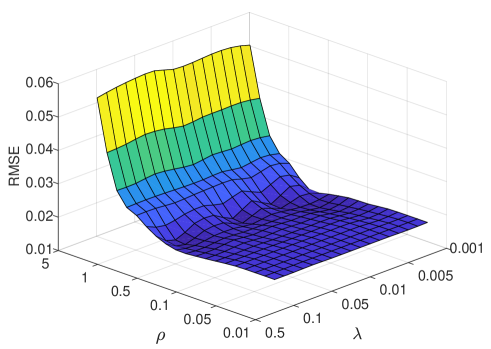
Figure 1: RMSE as a function of the regularization parameters for the Pro-H-NLM with synthetic data (SNR = 20 dB).

Table I shows the RMSE results of FCLS, SUnSAL-TV, CsUnL0, SCHU and our proposed PnP priors based unmixing methods. As we can see, for the synthetic data, RMSE results of the proposed framework show superiority compared to the other methods, especially when data SNRs are low. This indicates the effectiveness of priors excavated by denoisers. Whereas FCLS is a pixel-based unmixing method and it ignores the spatial-spectral correlations of natural hyperspectral images; SUnSAL-TV considers the spatial smooth information in the optimization problem. However, this method only considers the similarity of the four neighbors of a pixel. On the other hand, it neglects the variability information across spectral bands. CsUnL0 has no regard for the spatial information in the hyperspectral image, and SCHU does not introduce the spectral priors. All these compared methods use fixed regularizers and lack flexibility, while the proposed framwork does not need to handcraft regularizers and models the priors with the help of various denoisers. We can also observe that the unmixing results of denoisers plugged in the reconstructed image are better than denoisers plugged in the abundance maps. In other words, the features captured form the reconstructed image can effectively enhance the unmixing performance compared with the features captured form the abundance maps. Figure 2 presents the abundance maps of four compared methods, Pro-H-NLM, Pro-H-BM3D, Pro-H-BM4D and Pro-H-LRTDTV, with 5 dB data. In Figure 3, we present the abundance maps of four compared methods, Pro-A-NLM, Pro-A-BM3D, Pro-A-BM4D and Pro-A-DnCNN, with 10 dB data. We can observe that all the estimated abundance maps are consistent with the ground-truth. However, the abundance maps of our methods are with less noise and more close to ground-truth.

In addition, the PSNR results are also shown in Table I to demonstrate the impact of denoisers and show the superiority of our proposed framework. These results show that our proposed methods enhance the unmixing performance with priors form clean latent hyperspectral images by the application of denoisers. In Figure 4, we present the image reconstructed by the abundances and endmembers with LMM of different bands using the synthetic data with 10 dB. It is clear that our reconstructed images are cleaner compared with original noisy data and closer to the clean data. Using denoisers allows our method to maintain good unmixing performance when SNR is low. When SNR is high, the unmixing performance is still satisfactory, but the effect of denoisers is slight. The synthetic experiments confirm the applicability of our proposed methods from both quantitative and qualitative aspects.

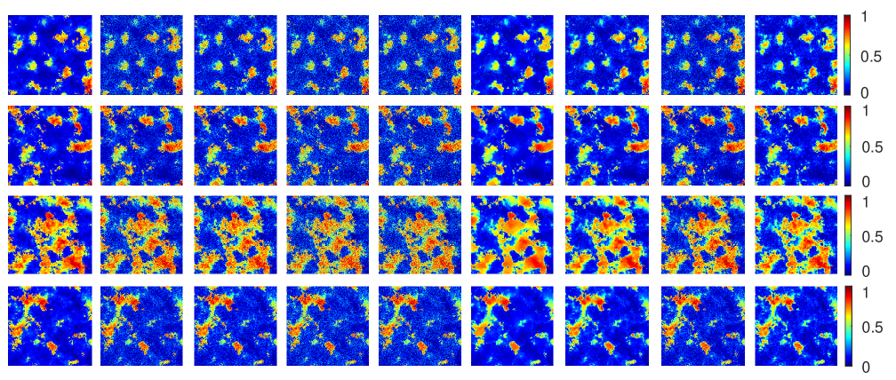
Figure 2: Abundance maps of synthetic data (SNR=5dB). From top to bottom: different endmembers. From left to right: ground-truth, FCLS, SUnSAL-TV, CsUnL0, SCHU, Pro-H-NLM, Pro-H-BM3D, Pro-H-BM4D, and Pro-H-LRTDTV.

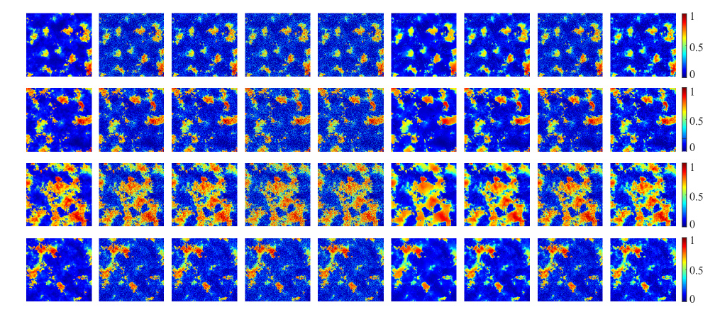
Figure 3: Abundance maps of synthetic data (SNR=10dB). From top to bottom: different endmembers. From left to right: ground-truth, FCLS, SUnSAL-TV, CsUnL0, SCHU, Pro-A-NLM, Pro-A-BM3D, Pro-A-BM4D, and Pro-A-DnCNN.

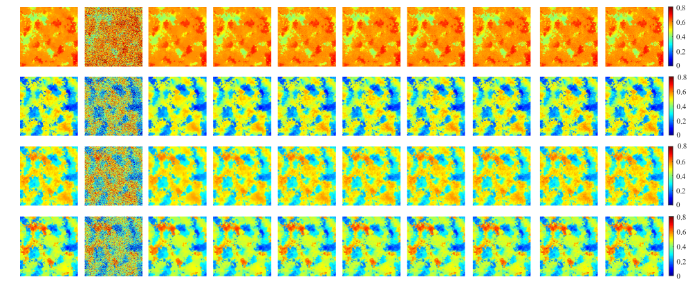
Figure 4: The reconstructed image maps. From top to bottom: reconstructed images in different channels (50, 100, 150, 200). From left to right: clean image, noisy image, reconstructed images of Pro-H-NLM, Pro-H-BM3D, Pro-H-BM4D, Pro-H-LRTDTV, Pro-A-NLM, Pro-A-BM3D, Pro-A-BM4D, and Pro-A-DnCNN.

IV-A3 Convergence Analysis

It is well known that a standard ADMM algorithm is guaranteed to converge [47, 48]. However, in our work, we use a denoiser as a black-box to replace the explicitly solving the second subproblem (18), and thus the convergence of this operator is difficult to analysis. In [37], the convergence of the PnP priors approach based on the linear filter, such as NLM, has been proved. For non-linear denoisers involving amounts of complex operators (e.g., BM3D and DnCNN), it is hard to prove the convergence of the proposed method theoretically. In practice, we observe the convergence curves of our proposed ADMM-based unmixing scheme involving both linear and non-linear denoisers to show its good convergence property.

Figure 8 illustrates the RMSE convergence curves of synthetic data of our proposed unmixing methods with different SNRs. It can be observed that the proposed ADMM-based framework with each denoising algorithm (both linear and non-linear) has a stable and robust convergence property. Moreover, the proposed method with all the deniosers achieve a low RMSE after 3 iterations, which indicates that an early stop operator can be considered for less computation time.

IV-B Experiments with Real Hyperspectral Dataset

Previous experiments were based on synthetic data, which can avoid extra errors caused by atmospheric or camera effects. However, hyperspectral unmixing methods are designed to be applied directly on real hyperspectral images. In this subsection, we use two real data to further verify the effectiveness of our proposed methods.

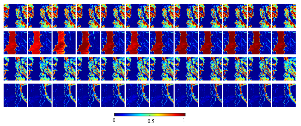
Figure 5: Abundance maps of Jasper Ridge dataset. From top to bottom: four endmembers, tree, water, soil, and road. From left to right: FCLS, SUnSAL-TV, CsUnL0, SCHU, Pro-H-NLM, Pro-H-BM3D, Pro-H-BM4D, Pro-H-LRTDTV, Pro-A-NLM, Pro-A-BM3D, Pro-A-BM4D, and Pro-A-DnCNN.

IV-B1 Data Description

The first dataset is Jasper Ridge dataset which was obtained by the Airborne Visible Infrared Imaging Spectrometer (AVIRIS). The original size of this data is $512\times 614$, with $224$ spectral bands. Following the previous unmixing works[49], we removed the noisy and water vapor absorption bands (1-3, 108-112, 154-166 and 220-224) of this data with 198 exploitable bands remained. An interest subset of $100\times 100$ size was selected to evaluate the unmixing performance. The color image of this dataset is shown in the left of Figure 6. There are four main endmembers in this dataset, including “tree”, “water”, “soil” and “road”. The endmembers used for this experiment were download from the website.

The second real hyperspectral dataset used for real hyperspectral image experiments is Urban dataset. The Urban dataset is of size $307\times 307$. The original Urban dataset consists of 210 bands, ranging from 400 nm to 2500 nm. We removed the water absorption and noisy channels (1-4, 76, 87, 101-111, 136-153, 198-210) in our experiment with 162 exploitable bands remained. Six endmembers, including “asphalt”, “grass”, “tree”, “roof”, “metal” and “dirt”, are extracted for this experiment. The endmembers used for this experiment was also download from the website${}^{\text{3}}$. The color image of this dataset is shown in the right of Figure 6.

For real hyperspectral dataset, it is impossible to obtain a dataset with the ground-truth of abundances to train the supervised denoising method DnCNN. We directly use the denoising network with parameters trained by natural image datasets.

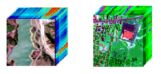
Figure 6: Color image of real dataset, Jasper Ridge dataset (left), Urban dataset (right).

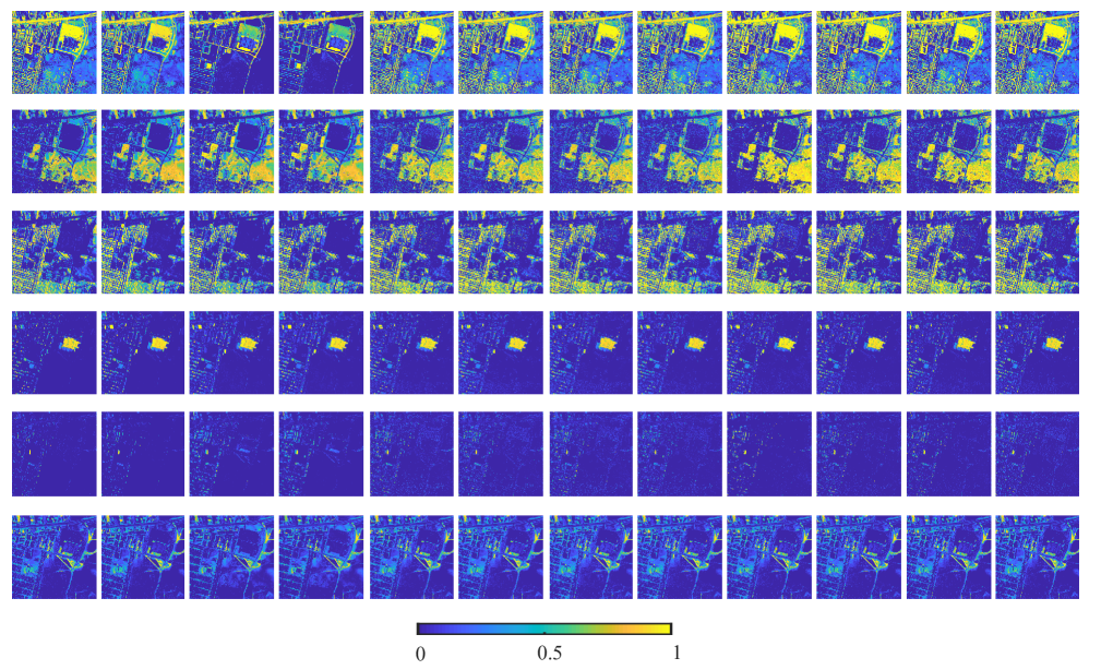
Figure 7: Abundance maps of Urban dataset. From top to bottom: six endmembers, asphalt, grass, tree, roof, metal, and dirt. From left to right: FCLS, SUnSAL-TV, CsUnL0, SCHU, Pro-H-NLM, Pro-H-BM3D, Pro-H-BM4D, Pro-H-LRTDTV, Pro-A-NLM, Pro-A-BM3D, Pro-A-BM4D, and Pro-A-DnCNN.

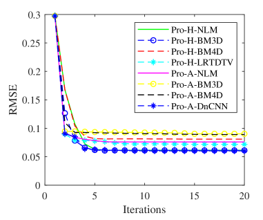
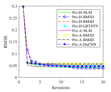
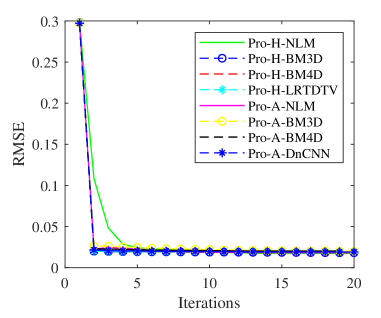
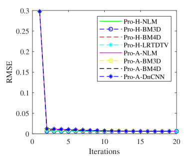
Figure 8: The RMSE convergence curves of synthetic data of our proposed methods with different SNRs. From left to right, top to bottom: SNR=5 dB, 10 dB, 20 dB and 30 dB, respectively.

IV-B2 Unmixing Results and Discussion

The parameter settings of these experiments are the same as the synthetic data. Figure 5 presents the abundance maps of different methods of the Jasper Ridge dataset. The unmixing results of our proposed methods show the most smooth and clear abundance maps, especially the unmixing results of the material “water”. For the material “road”, our methods can emphasize some locations and provide sharper maps. The abundance maps of the Urban dataset are shown in Figure 7. This dataset is more complex and increases the difficulty of unmixing. A visual comparison of these methods indicates that our methods preserve more spatial homogeneous information and contain more details. From Figure 7, we see that our methods provide clear and smooth abundance maps while CsUnL0 and SCHU fail to unmix this dataset with the material “asphalt”. All unmixing results of this two real datasets confirm that our PnP priors based framework for hyperspectral unmixing provides superior unmixing performance.

We use the reconstructed error (RE) to give a quantitative evaluation of the unmixing results of real data. RE is defined as:

$$\text{RE}=\sqrt{\frac{1}{NL}\sum_{i=1}^{N}\|\mathbf{y}_{i}-\mathbf{\hat{y}}_{i}\|^{2}},$$ (27)

where $\mathbf{y}_{i}$ is the $i$-th pixel and $\mathbf{\hat{y}}_{i}$ is its reconstruction. Note that the RE results are not necessarily proportional to the quality of the abundance estimation, and therefore it can only be considered as complementary information. Table II shows the RE results of Jasper Ridge dataset. Table III presents the RE results of Urban dataset. We can see that the RE results are all in an order of magnitude. As the noise are unavoidable in real data, and the proposed framework can effectively denoise the data, the RE results of the proposed methods are easily larger than compared methods. The maps of reconstructed error of Jasper Ridge dataset and Urban dataset are shown in Figure 9 and Figure 10, respectively.

TABLE II: RE Comparison of Jasper Ridge dataset.

	FCLS	SUnSAL-TV	CsUnL0	SCHU	Pro-H-NLM	Pro-H-BM3D
RE	0.0281	0.0157	0.0166	0.0166	0.0301	0.0312
	Pro-H-BM4D	Pro-H-LRTDTV	Pro-A-NLM	Pro-A-BM3D	Pro-A-BM4D	Pro-A-DnCNN
RE	0.0296	0.0300	0.0363	0.0315	0.0367	0.0304

TABLE III: RE Comparison of Urban dataset.

	FCLS	SUnSAL-TV	CsUnL0	SCHU	Pro-H-NLM	Pro-H-BM3D
RE	0.0411	0.0183	0.0144	0.0145	0.0555	0.0550
	Pro-H-BM4D	Pro-H-LRTDTV	Pro-A-NLM	Pro-A-BM3D	Pro-A-BM4D	Pro-A-DnCNN
RE	0.0559	0.0540	0.0514	0.0493	0.0529	0.0540

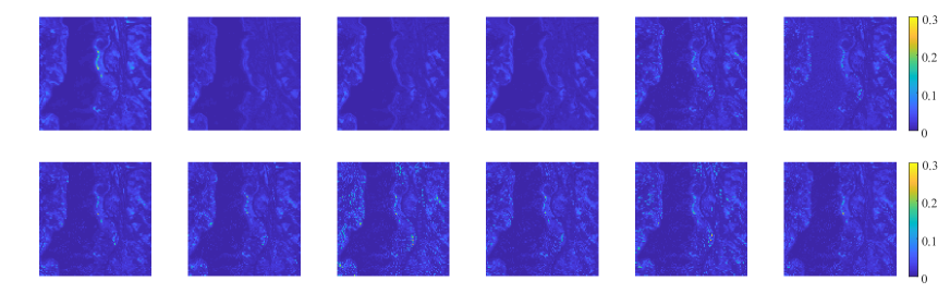
Figure 9: Maps of reconstructed error of Jasper Ridge dataset. From left to right, top to bottom: FCLS, SUnSAL-TV, CsUnL0, SCHU, Pro-H-NLM, Pro-H-BM3D, Pro-H-BM4D, Pro-H-LRTDTV, Pro-A-NLM, Pro-A-BM3D, Pro-A-BM4D and Pro-A-DnCNN.

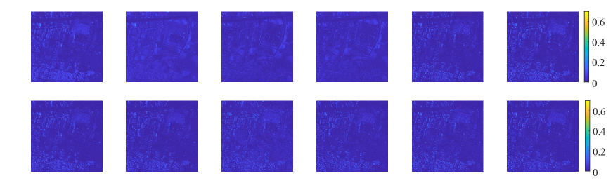
Figure 10: Maps of reconstructed error of Urban dataset. From left to right, top to bottom: FCLS, SUnSAL-TV, CsUnL0, SCHU, Pro-H-NLM, Pro-H-BM3D, Pro-H-BM4D, Pro-H-LRTDTV, Pro-A-NLM, Pro-A-BM3D, Pro-A-BM4D and Pro-A-DnCNN.

IV-C Running Time

To weigh the trade-off between performance gain and computational burden, we conduct experiments for evaluating the running time using different datasets. We set the number of iteration $K=20$. Note that all the experiments are conducted on the computer with Intel i7-8700 3.2-Ghz CPU and 16-GB random access memory. Table IV, Table V and Table VI present the average computing time of synthetic data, Jasper Ridge dataset and Urban dataset. We observe that the running time of the proposed framework mainly depends on the complexity of denoisers. The convergence speed of 2D denoisers is faster than 3D counterparts. Denoising abundance maps is faster than denoising hyperspectral images.

TABLE IV: Time consuming of the proposed methods for synthetic data (seconds).

	Pro-H-NLM	Pro-H-BM3D	Pro-H-BM4D	Pro-H-LRTDTV
time	288	374	6314	3247
	Pro-A-NLM	Pro-A-BM3D	Pro-A-BM4D	Pro-A-DnCNN
time	23	25	47	771

TABLE V: Time consuming of the proposed methods for Jasper Ridge dataset (seconds).

	Pro-H-NLM	Pro-H-BM3D	Pro-H-BM4D	Pro-H-LRTDTV
time	48	53	1497	439
	Pro-A-NLM	Pro-A-BM3D	Pro-A-BM4D	Pro-A-DnCNN
time	4	4	8	192

TABLE VI: Time consuming of the proposed methods for Urban dataset (seconds).

	Pro-H-NLM	Pro-H-BM3D	Pro-H-BM4D	Pro-H-LRTDTV
time	315	403	5879	3399
	Pro-A-NLM	Pro-A-BM3D	Pro-A-BM4D	Pro-A-DnCNN
time	37	44	191	1531

V Conclusion

In this paper, we propose a PnP priors based framework for hyperspectral unmixing, which is flexible and extendable by using various image denoisers. The proposed framework makes full use of the spatial-spectral priors of hyperspectral images and abundance maps. It is easy to switch the pattern of imposing the penalty on reconstructed hyperspectral images or abundance maps by different choices of matrix $\mathbf{H}$. Various denoisers, including linear, non-linear, or deep learning based denoisers are used to excavate the priors. Our proposed unmixing framework with all these denoisers have a good convergence property. Experiment results of both synthetic data and real data show that our framework achieves superior unmixing performance. Also, it indicates the effectiveness of excavated priors via denoisers. In future work, we will focus on how to automatically select the parameters $\rho$ and $\lambda$. Moreover, we will conduct the PnP priors framework for jointly deblurring and unmixing hyperspectral images.

References

- [1] X. Wang, M. Zhao, and J. Chen, “Hyperspectral unmixing via plug-and-play priors,” in 2020 IEEE International Conference on Image Processing (ICIP). IEEE, 2020, pp. 1063–1067.
- [2] D. W. Stein, S. G. Beaven, L. E. Hoff, E. M. Winter, A. P. Schaum, and A. D. Stocker, “Anomaly detection from hyperspectral imagery,” IEEE Signal Proc. Mag., vol. 19, no. 1, pp. 58–69, 2002.
- [3] C.-I. Chang and Q. Du, “Estimation of number of spectrally distinct signal sources in hyperspectral imagery,” IEEE Trans. Geosci. Remote Sens., vol. 42, no. 3, pp. 608–619, 2004.
- [4] M. Fauvel, Y. Tarabalka, J. A. Benediktsson, J. Chanussot, and J. C. Tilton, “Advances in spectral-spatial classification of hyperspectral images,” Proc. of the IEEE, vol. 101, no. 3, pp. 652–675, 2012.
- [5] X. Yang, J. Chen, and Z. He, “Sparse-spatialcem for hyperspectral target detection,” IEEE J. Sel. Top. Appl. Earth Observat. Remote Sens., vol. 12, no. 7, pp. 2184–2195, 2019.
- [6] R. Heylen, M. Parente, and P. Gader, “A review of nonlinear hyperspectral unmixing methods,” IEEE J. Sel. Top. Appl. Earth Observat. Remote Sens., vol. 7, no. 6, pp. 1844–1868, 2014.
- [7] J. M. Bioucas-Dias, A. Plaza, N. Dobigeon, M. Parente, Q. Du, P. Gader, and J. Chanussot, “Hyperspectral unmixing overview: Geometrical, statistical, and sparse regression-based approaches,” IEEE J. Sel. Top. Appl. Earth Observat. Remote Sens., vol. 5, no. 2, pp. 354–379, 2012.
- [8] N. Dobigeon, S. Moussaoui, M. Coulon, J.-Y. Tourneret, and A. O. Hero, “Joint bayesian endmember extraction and linear unmixing for hyperspectral imagery,” IEEE Trans. Signal Process., vol. 57, no. 11, pp. 4355–4368, 2009.
- [9] S. Yang, X. Zhang, Y. Yao, S. Cheng, and L. Jiao, “Geometric nonnegative matrix factorization (gnmf) for hyperspectral unmixing,” IEEE J. Sel. Top. Appl. Earth Observat. Remote Sens., vol. 8, no. 6, pp. 2696–2703, 2015.
- [10] J. Yuan, Y. Zhang, and F. Gao, “An overview on linear hyperspectral unmixing,” J. Infrared Millim. Waves, vol. 37, pp. 553–571, 2018.
- [11] L. Drumetz, M.-A. Veganzones, S. Henrot, R. Phlypo, J. Chanussot, and C. Jutten, “Blind hyperspectral unmixing using an extended linear mixing model to address spectral variability,” IEEE Trans. Image Process., vol. 25, no. 8, pp. 3890–3905, 2016.
- [12] D. Hong, N. Yokoya, J. Chanussot, and X. X. Zhu, “An augmented linear mixing model to address spectral variability for hyperspectral unmixing,” IEEE Trans. Image Process., vol. 28, no. 4, pp. 1923–1938, 2018.
- [13] J. Chen, C. Richard, and P. Honeine, “Nonlinear unmixing of hyperspectral data based on a linear-mixture/nonlinear-fluctuation model,” IEEE Trans. Signal Process., vol. 61, no. 2, pp. 480–492, 2012.
- [14] D. C. Heinz et al., “Fully constrained least squares linear spectral mixture analysis method for material quantification in hyperspectral imagery,” IEEE Trans. Geosci. Remote Sens., vol. 39, no. 3, pp. 529–545, 2001.
- [15] A. Halimi, J. M. Bioucas-Dias, N. Dobigeon, G. S. Buller, and S. McLaughlin, “Fast hyperspectral unmixing in presence of nonlinearity or mismodeling effects,” IEEE Trans. Comput. Imaging, vol. 3, no. 2, pp. 146–159, 2016.
- [16] R. Ammanouil, A. Ferrari, and C. Richard, “A graph laplacian regularization for hyperspectral data unmixing,” in 2015 IEEE International Conference on Acoustics, Speech and Signal Processing (ICASSP). IEEE, 2015, pp. 1637–1641.
- [17] ——, “Hyperspectral data unmixing with graph-based regularization,” in 2015 7th Workshop on Hyperspectral Image and Signal Processing: Evolution in Remote Sensing (WHISPERS). IEEE, 2015, pp. 1–4.
- [18] M.-D. Iordache, J. M. Bioucas-Dias, and A. Plaza, “Total variation spatial regularization for sparse hyperspectral unmixing,” IEEE Trans. Geosci. Remote Sens., vol. 50, no. 11, pp. 4484–4502, 2012.
- [19] R. Wang, H.-C. Li, A. Pizurica, J. Li, A. Plaza, and W. J. Emery, “Hyperspectral unmixing using double reweighted sparse regression and total variation,” IEEE Geosci. Remote Sens. Lett., vol. 14, no. 7, pp. 1146–1150, 2017.
- [20] W. He, H. Zhang, and L. Zhang, “Total variation regularized reweighted sparse nonnegative matrix factorization for hyperspectral unmixing,” IEEE Trans. Geosci. Remote Sens., vol. 55, no. 7, pp. 3909–3921, 2017.
- [21] R. Feng, Y. Zhong, Y. Wu, D. He, X. Xu, and L. Zhang, “Nonlocal total variation subpixel mapping for hyperspectral remote sensing imagery,” Remote Sensing, vol. 8, no. 3, p. 250, 2016.
- [22] Y. Zhong, R. Feng, and L. Zhang, “Non-local sparse unmixing for hyperspectral remote sensing imagery,” IEEE J. Sel. Top. Appl. Earth Observat. Remote Sens., vol. 7, no. 6, pp. 1889–1909, 2013.
- [23] J. Yao, D. Meng, Q. Zhao, W. Cao, and Z. Xu, “Nonconvex-sparsity and nonlocal-smoothness-based blind hyperspectral unmixing,” IEEE Trans. Image Process., vol. 28, no. 6, pp. 2991–3006, 2019.
- [24] X. Wang, Y. Zhong, L. Zhang, and Y. Xu, “Spatial group sparsity regularized nonnegative matrix factorization for hyperspectral unmixing,” IEEE Trans. Geosci. Remote Sens., vol. 55, no. 11, pp. 6287–6304, 2017.
- [25] Z. Li, J. Chen, and S. Rahardja, “Superpixel construction for hyperspectral unmixing,” in 2018 26th European Signal Processing Conference (EUSIPCO). IEEE, 2018, pp. 647–651.
- [26] S. Zhang, J. Li, H.-C. Li, C. Deng, and A. Plaza, “Spectral–spatial weighted sparse regression for hyperspectral image unmixing,” IEEE Trans. Geosci. Remote Sens., vol. 56, no. 6, pp. 3265–3276, 2018.
- [27] D. Hong and X. X. Zhu, “Sulora: Subspace unmixing with low-rank attribute embedding for hyperspectral data analysis,” IEEE J. Sel. Top. Sig. Process., vol. 12, no. 6, pp. 1351–1363, 2018.
- [28] B. Palsson, M. O. Ulfarsson, and J. R. Sveinsson, “Convolutional autoencoder for spatial-spectral hyperspectral unmixing,” in 2019 IEEE International Geoscience and Remote Sensing Symposium (IGARSS). IEEE, 2019, pp. 357–360.
- [29] F. Khajehrayeni and H. Ghassemian, “Hyperspectral unmixing using deep convolutional autoencoders in a supervised scenario,” IEEE J. Sel. Top. Appl. Earth Observat. Remote Sens., vol. 13, pp. 567–576, 2020.
- [30] X. Zhang, Y. Sun, J. Zhang, P. Wu, and L. Jiao, “Hyperspectral unmixing via deep convolutional neural networks,” IEEE Geosci. Remote Sens. Lett., vol. 15, no. 11, pp. 1755–1759, 2018.
- [31] B. Lin, X. Tao, and J. Lu, “Hyperspectral image denoising via matrix factorization and deep prior regularization,” IEEE Trans. Image Process., vol. 29, pp. 565–578, 2019.
- [32] “Hyperspectral image denoising and anomaly detection based on low-rank and sparse representations,” in Image and Signal Processing for Remote Sensing, 2017.
- [33] D. Gong, Z. Zhang, Q. Shi, A. v. d. Hengel, C. Shen, and Y. Zhang, “Learning an optimizer for image deconvolution,” arXiv preprint arXiv:1804.03368, 2018.
- [34] X. Wang, J. Chen, C. Richard, and D. Brie, “Learning spectral-spatial prior via 3DDnCNN for hyperspectral image deconvolution,” in 2020 45th IEEE International Conference on Acoustics, Speech and Signal Processing (ICASSP). IEEE, 2020, pp. 2403–2407.
- [35] A. Teodoro, J. Bioucas-Dias, and M. Figueiredo, “Sharpening hyperspectral images using plug-and-play priors,” in International Conference on Latent Variable Analysis and Signal Separation. Springer, 2017, pp. 392–402.
- [36] A. M. Teodoro, J. M. Bioucas-Dias, and M. A. Figueiredo, “Scene-adapted plug-and-play algorithm with convergence guarantees,” in 2017 IEEE 27th International Workshop on Machine Learning for Signal Processing (MLSP). IEEE, 2017, pp. 1–6.
- [37] S. Sreehari, S. V. Venkatakrishnan, B. Wohlberg, G. T. Buzzard, L. F. Drummy, J. P. Simmons, and C. A. Bouman, “Plug-and-play priors for bright field electron tomography and sparse interpolation,” IEEE Trans. Comput. Imaging, vol. 2, no. 4, pp. 408–423, 2016.
- [38] A. M. Teodoro, J. M. Bioucas-Dias, and M. A. Figueiredo, “Image restoration and reconstruction using targeted plug-and-play priors,” IEEE Trans. Comput. Imaging, vol. 5, no. 4, pp. 675–686, 2019.
- [39] S. Boyd, N. Parikh, E. Chu, B. Peleato, J. Eckstein et al., “Distributed optimization and statistical learning via the alternating direction method of multipliers,” Found. Trends Mach. Learn., vol. 3, no. 1, pp. 1–122, 2011.
- [40] Y. Bai, W. Chen, J. Chen, and W. Guo, “Deep learning methods for solving linear inverse problems: Research directions and paradigms,” Signal Processing, p. 107729, 2020.
- [41] A. Buades, B. Coll, and J.-M. Morel, “Non-local means denoising,” Image Processing On Line, vol. 1, pp. 208–212, 2011.
- [42] K. Dabov, A. Foi, V. Katkovnik, and K. Egiazarian, “Image denoising by sparse 3-d transform-domain collaborative filtering,” IEEE Trans. Image Process., vol. 16, no. 8, pp. 2080–2095, 2007.
- [43] M. Maggioni, V. Katkovnik, K. Egiazarian, and A. Foi, “Nonlocal transform-domain filter for volumetric data denoising and reconstruction,” IEEE Trans. Image Process., vol. 22, no. 1, pp. 119–133, 2012.
- [44] Y. Wang, J. Peng, Q. Zhao, Y. Leung, X.-L. Zhao, and D. Meng, “Hyperspectral image restoration via total variation regularized low-rank tensor decomposition,” IEEE J. Sel. Top. Appl. Earth Observat. Remote Sens., vol. 11, no. 4, pp. 1227–1243, 2017.
- [45] K. Zhang, W. Zuo, Y. Chen, D. Meng, and L. Zhang, “Beyond a gaussian denoiser: Residual learning of deep cnn for image denoising,” IEEE Trans. Image Process., vol. 26, no. 7, pp. 3142–3155, 2017.
- [46] Z. Shi, T. Shi, M. Zhou, and X. Xu, “Collaborative sparse hyperspectral unmixing using norm,” IEEE Trans. Geosci. Remote Sens., vol. 56, no. 9, pp. 5495–5508, 2018.
- [47] J. Eckstein and D. P. Bertsekas, “On the Douglas–Rachford splitting method and the proximal point algorithm for maximal monotone operators,” Mathematical Programming, vol. 55, no. 1-3, pp. 293–318, 1992.
- [48] M. V. Afonso, J. M. Bioucas-Dias, and M. A. Figueiredo, “Fast image recovery using variable splitting and constrained optimization,” IEEE Trans. Image Process., vol. 19, no. 9, pp. 2345–2356, 2010.
- [49] H. K. Aggarwal and A. Majumdar, “Hyperspectral unmixing in the presence of mixed noise using joint-sparsity and total variation,” IEEE J. Sel. Top. Appl. Earth Observat. Remote Sens., vol. 9, no. 9, pp. 4257–4266, 2016.