Constructing tensor network wavefunction for a generic two-dimensional quantum phase transition via thermofield double states

Abstract

The most important feature of two-dimensional quantum Rokhsar-Kivelson (RK) type models is that their ground state wavefunction norms can be mapped into the partition functions of two-dimensional statistical models so that the quantum phase transitions become the thermal phase transitions of the corresponding statistical models. For a generic quantum critical point, we generalize the framework of RK wavefunctions by introducing the concept of the thermofield double (TFD) state, which is a purification of the equilibrium density operator. Moreover, by expressing the TFD state in terms of the projected entangled pair state, its $N$-order of Rényi entropy results in a three-dimensional statistical model in Euclidian spacetime, describing the generic quantum phase transitions. Using the toric code model with two parallel magnetic fields as an example, we explain these ideas and derive the partition function of the three-dimensional $Z_{2}$ lattice gauge-Higgs model, where the phase transitions are characterized by the three-dimensional universality classes.

Introduction. -Recently quantum spin liquids, topological phases of matter, and their quantum phase transitions have been attracted enormous research interest, and there has been a very active development of tensor network states to study these correlated quantum many-body phenomenaVerstraete et al. (2008); Schollwöck (2011); Orús (2014); Haegeman and Verstraete (2017). Since the ground states and low-energy excited states of two-dimensional (2D) quantum systems with local interactions are only weak entangled, the entanglement entropy of a region scales with its areaWolf et al. (2008); Eisert et al. (2010). Then infinite projected entangled-pair states (iPEPS) or tensor network statesVerstraete and Cirac (2004); Jordan et al. (2008); Nishino et al. (2001); Nishio et al. (2004) has become a powerful theoretical tool to characterize those correlated quantum many-body phases in the thermodynamic limitSchuch et al. (2012, 2013). However, there still exists an open problem how well the iPEPS can describe two-dimensional quantum critical states emerging at the quantum critical pointsRader and Läuchli (2018a); Corboz et al. (2018a).

Since the norm of the iPEPS can be related to a partition function of classical statistical models, the zero-temperature quantum phase transitions can be mapped to the temperature-driven classical phase transitionsIsakov et al. (2011); Haegeman et al. (2015); Zhu and Zhang (2019); Xu et al. (2020), and there is a class of exact 2D critical iPEPS with a small value of bond dimension, describing the ground states of the generalized Rokhsar-Kivelson (RK) Hamiltonians at their critical pointArdonne et al. (2004); Castelnovo et al. (2005); Verstraete et al. (2006). However, a generic 2D quantum phase transition should be described by the partition function of a 3D classical statistical model in the Euclidian space, where an extra dimension corresponds to the ”imaginary time” to represent thermal fluctuations at the critical point. And the emerging critical properties of the 2D quantum model belong to the same universality class as that of the 3D classical system. Therefore, the most important question is to establish a general framework connecting the tensor network wavefunction for a 2D quantum system to a 3D classical partition function, and to find out the necessary conditions under which the general framework can be applied.

In this paper, we generalize the RK wavefunctions to the framework of the so-call thermofield double (TFD) statesTakahashi and Umezawa (1996), which are defined in an enlarged Hilbert space $\mathcal{H}_{P}\otimes\mathcal{H}_{F}$ consisting of the physical space $\mathcal{H}_{P}$ and a fictitious space $\mathcal{H}_{F}$. The TFD state is a purification of a mixed density operator in thermal equilibrium, and the thermal fluctuations is encoded in the form of quantum entanglement between the physical and fictitious parts. For a class of 2D quantum systems, their model Hamiltonians can be divided into two noncommutative parts $\hat{H}=\hat{H}^{(1)}+\hat{H}^{(2)}$ and each part is a sum of the commuting local terms. We can introduce a tensor network TFD state with variational parameters, and then a reduced TFD density operator can be obtained by integrating out the fictitious degrees of freedom. We prove that the $N$-th order Rényi entropy gives rise to the partition function of 3D statistical models in the Euclidian space, where the imaginary time dimension is discretized into $N$ layers. In the large $N$ limit, we expect that the phase transitions of the 3D statistical models characterize the quantum phase transitions in the 2D quantum model. As an example, we carefully study the toric code model in two parallel fieldsKitaev (2003); Vidal et al. (2009); Tupitsyn et al. (2010). By constructing a variational tensor network TFD state, we successfully derive the partition function of the 3D lattice gauge-Higgs modelFradkin and Shenker (1979); Jongeward et al. (1980); Tupitsyn et al. (2010), which can be used to describe the topological quantum phase transitions out of the toric code phase.

General framework. -From a 2D classical Hamiltonian $E(\sigma_{1},\cdots,\sigma_{n})$ with spin variables $\{\sigma_{i}\}$, the RK-type wavefunction with a parameter $\beta$ is defined by

$$|\psi(\beta)\rangle=\sum_{\bm{\sigma}}\text{e}^{-\beta E(\bm{\sigma})/2}|\bm{\sigma}\rangle.$$ (1)

where $|\bm{\sigma}\rangle=|\sigma_{1},\cdots,\sigma_{n}\rangle$ and $\{|\bm{\sigma}\rangle\}$ is a set of completely orthogonal basis. The wavefunction norm precisely corresponds to the partition function of a classical model with $\beta$ as the inverse temperature:

$$Z(\beta)=\langle\psi(\beta)|\psi(\beta)\rangle=\sum_{\bm{\sigma}}\exp[-\beta E(\bm{\sigma})].$$ (2)

With such a quantum-classical mapping, all equal-time correlation functions of local observable operators are mapped into the correlation functions of the classical partition function. Then the quantum phase transitions in the RK wavefunction are described by the partition function of a 2D classical model.

When we consider a 2D quantum Hamiltonian $\hat{H}(\hat{\sigma}_{i},\cdots,\hat{\sigma}_{n})$ with spin operators $\{\hat{\sigma}_{i}\}$, a generic quantum wavefunction function can be expressed as

$$|\Psi_{0}(\beta)\rangle=\sum_{\bm{\sigma}}e^{-\beta\hat{H}(\hat{\sigma}_{i}\cdots\hat{\sigma}_{n})/2}|\bm{\sigma}\rangle.$$ (3)

When $\beta\rightarrow\infty$, the wavefunction $|\Psi_{0}(\infty)\rangle$ approaches to the ground state of $\hat{H}$. Unlike the RK type wavefunctions, the norm of the wavefunction $\langle\Psi_{0}(\beta)|\Psi_{0}(\beta)\rangle$ is significantly different from the partition function of the quantum Hamiltonian $\mathcal{Z}(\beta)=\text{tr}e^{-\beta\hat{H}}$. The former sums over both diagonal and off-diagonal matrix elements of the density operator $e^{-\beta\hat{H}}$, the later is just a sum of diagonal matrix elements. So we can not make the norm of a pure state equivalent to the trace of a mixed state in the original Hilbert space, except the gapped system at zero temperature. However, in an enlarged Hilbert spaceTakahashi and Umezawa (1996), it can be done by constructing the so-called TFD state:

$$|\tilde{\Psi}_{0}(\beta)\rangle=\sum_{\bm{\sigma}}\left[e^{-\beta\hat{H}/2}|\bm{\sigma}\rangle_{P}\right]\otimes|\bm{\sigma}\rangle_{F},$$ (4)

where the enlarged Hilbert space $\mathcal{H}_{P}\otimes\mathcal{H}_{F}$ consists of the physical space $\mathcal{H}_{P}$ and a fictitious one $\mathcal{H}_{F}$, and the square root of the density operator acts on the physical space only. It is always sufficient to choose $\mathcal{H}_{F}$ to be identical to $\mathcal{H}_{P}$, “doubling” each degree of freedom. For a gapped quantum system with a non-degenerate ground state, the entanglement between the physical and fictitious parts decreases with increasing $\beta$. In the limit of $\beta\rightarrow\infty$, the density operator becomes a ground state projector, leading to a product state $|\tilde{\Psi}_{0}(\infty)\rangle=|\Psi_{0}(\infty)\rangle_{P}\otimes|\Psi_{0}^{\ast}(\infty)\rangle_{F}$. So for a gapped system at zero temperature, using the TFD state is not necessary. However, it is essential for a critical system to consider the entanglement between two parts of a TFD state.

Then tracing out the degrees of freedom in the fictitious space yields a reduced density matrix of the TFD state

$$\rho_{0}=\text{tr}_{F}|\tilde{\Psi}_{0}(\beta)\rangle\langle\tilde{\Psi}_{0}(\beta)|=e^{-\beta\hat{H}},$$ (5)

which is the exact Gibbs density operator. So the information of the thermal fluctuations is just encoded in the form of the quantum entanglement between the physical and fictitious parts, and the norm of the TFD state corresponds to the partition function of the 2D quantum Hamiltonian:

$$\mathcal{Z}(\beta)=\langle\tilde{\Psi}_{0}(\beta)|\tilde{\Psi}_{0}(\beta)\rangle=\text{tr}e^{-\beta\hat{H}}.$$ (6)

Therefore, the TFD state reconciles the norm and trace operations and generalizes the RK-type wavefunctions, and the unequal time correlation function can be calculated with the TFD states.

Usually it is very hard to express the wavefunction coefficients as the products of local Boltzmann weightsVerstraete et al. (2006); Molnar et al. (2015). For a special class of quantum systems, however, their model Hamiltonians can be divided into two noncommutative parts $\hat{H}=\hat{H}^{(1)}+\hat{H}^{(2)}$ and each part is a sum of the commuting local terms. Then a good variational ground state wavefunction can be expressed asVanderstraeten et al. (2017)

$$|\Psi(\alpha_{1},\alpha_{2})\rangle=\sum_{\bm{\sigma}}e^{-\alpha_{1}\hat{H}^{(1)}/2}e^{-\alpha_{2}\hat{H}^{(2)}/2}|\bm{\sigma}\rangle,$$ (7)

where $(\alpha_{1},\alpha_{2})$ are two variational parameters. Then we can express the corresponding TFD state as

$$|\tilde{\Psi}(\alpha_{1},\alpha_{2})\rangle=\sum_{\bm{\bar{\sigma}},\bm{\sigma}}(e^{-\alpha_{1}\hat{H}^{(1)}/2}e^{-\alpha_{2}\hat{H}^{(2)}/2})_{\bar{\sigma}{\sigma}}|\bm{\bar{\sigma}}\rangle_{P}\otimes|\bm{\sigma}\rangle_{F},$$ (8)

and those coefficients can be easily written as the products of local Boltzmann weights

$$(e^{-\alpha_{1}\hat{H}^{(1)}/2}e^{-\alpha_{2}\hat{H}^{(2)}/2})_{\bar{\sigma}{\sigma}}=\sum_{\bm{s}}\prod_{v}\exp\left[{-\epsilon_{s_{v}}^{\sigma_{v},\bar{\sigma}_{v}}(\alpha_{1},\alpha_{2})}\right],$$

where the auxiliary degrees of freedom $\bm{s}=s_{1},\cdots,s_{m}$ have been introduced and $\sigma_{v},s_{v},\bar{\sigma}_{v}$ are the sets of spin variables belonging to the vertex $v$. When the local Boltzmann weights are replaced by local tensors, the TFD state wavefunction becomes an iPEPS with physical degrees of freedom $\bm{\bar{\sigma}},\bm{\sigma}$.

From Eq. (8), after integrating out the fictitious degrees of freedom, we obtain a reduced TFD density operator

$$\rho=\text{tr}_{F}|\tilde{\Psi}\rangle\langle\tilde{\Psi}|=e^{-\alpha_{1}\hat{H}^{(1)}/2}e^{-\alpha_{2}\hat{H}^{((2)}}e^{-\alpha_{1}\hat{H}^{(1)}/2}.$$ (9)

In order to construct the partition function of a 3D statistical model for the critical iPEPS, we stack $N$ copies of $\rho$ and contract all degrees of freedom including those at the top of the $N$-th layer and those at the first layer. Then we identify $\mathcal{Z}_{N}=$tr$\rho^{N}$ as a partition function in the Euclidian spacetime. Actually the usual $N$-th order Rényi entropy is given by

$$S_{N}=\frac{\log\text{tr}\rho^{N}}{1-N}.$$ (10)

So the derived partition function $\mathcal{Z}_{N}$ can be explicitly written in terms of the local tensors of the iPEPS,

$$\mathcal{Z}_{N}=\sum_{\begin{subarray}{c}\bm{\sigma}_{1}^{[1]}\cdots\bm{\sigma}_{n}^{[N]},\\ \bm{s}_{1}^{[1]}\cdots\bm{s}_{1}^{[N]}\end{subarray}}\exp\left[{-\sum_{\tau=1}^{N}\sum_{v}\epsilon_{s_{v}^{[\tau]}}^{\sigma_{v}^{[\tau]},\sigma_{v}^{[\tau+1]}}(2\alpha_{1},2\alpha_{2})}\right],$$ (11)

where $\tau$ denotes the discretized imaginary time. When $N$ is sufficient large, the quantum-classical mapping of the RK-type wavefunction is thus generalized by using the concept of the TFD state via quantum entanglement, and the partition function of a 2D quantum system is transformed into that of a 3D classical one, which can be simulated with the classical resources. If the intra-layer interactions in the spatial directions have the same form as the inter-layer interactions in the imaginary time direction, the isotropic 3D model at the critical point has an emergent Lorentz symmetry and the dynamical critical exponent $z=1$.

Toric code model in two parallel fields. -To illustrate the above general theory, we consider the toric code model defined on a square lattice

$$H_{\text{TC}} = -\sum_{v}A_{v}-\sum_{p}B_{p},$$ (12)

$$A_{v} = -\sum_{v}\prod_{\langle ij\rangle\in v}\sigma_{ij}^{x},\quad B_{p}=-\sum_{p}\prod_{\langle ij\rangle\in p}\sigma_{ij}^{z},$$

where the vertex and plaquette terms $A_{v}$ and $B_{p}$ involve four Pauli spin-1/2 operators located on the bonds between sites $i$ and $j$. $A_{v}=-1$ is associated with an electric charge excitation, while $B_{p}=-1$ is associated with a magnetic flux excitation. The ground states can be projected out by the projectors of the subspaces:

$$|\Psi_{\text{TC}}^{m}\rangle=\prod_{v}\left(1+A_{v}\right)|\uparrow\rangle^{\otimes L},\text{ }|\Psi_{\text{TC}}^{e}\rangle=\prod_{p}\left(1+B_{p}\right)|+\rangle^{\otimes L}.$$

where $|+\rangle=(|\uparrow\rangle+|\downarrow\rangle)/\sqrt{2}$ and $L$ is the bond number. On a manifold with the trivial topology, the ground state is non-degenerate, $|\Psi_{\text{TC}}^{e}\rangle=|\Psi_{\text{TC}}^{m}\rangle$.

It is useful to represent the ground states as iPEPS. When auxiliary degrees of freedom $s_{j}=\pm 1$ on each site is introduced, the off-diagonal projector can be expressed as a projected entangled pair operator (PEPO)

$$\prod_{v}\left(1+A_{v}\right)=\sum_{\bm{s}\bm{\sigma}\bm{\bar{\sigma}}}\prod_{ij}\frac{1+s_{i}s_{j}\sigma_{ij}\bar{\sigma}_{ij}}{2}|\bm{\sigma}\rangle\langle\bm{\bar{\sigma}}|,$$

corresponding to a double-line PEPO on the dual lattice in Fig. 1 (a), while the diagonal projector is just a single line PEPO on the dual lattice

$$\prod_{p}\left(1+B_{p}\right)=\sum_{\bm{\sigma}}\prod_{\hat{v}}\left[1+\prod_{\langle ij\rangle\in\hat{v}}\sigma_{ij}\right]|\bm{\sigma}\rangle\langle\bm{\sigma}|,$$

with $\hat{v}=p$ as a vertex of the dual lattice, as shown in Fig. 1(b).

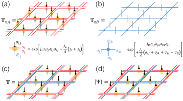
Figure 1: (a) The double-line PEPO representation of $\mathbb{T}_{xA}$ and a local tensor on a bond. When this PEPO is reduced to an off-diagonal projector, the local tensor becomes $({1+s_{i}s_{j}\sigma_{ij}\bar{\sigma}_{ij}})/2$. (b) The single-line PEPO representation of $\mathbb{T}_{zB}$ and a local tensor on the vertex $\hat{v}$. When this PEPO is reduced to the diagonal projector, the local tensor becomes $1+\sigma_{ij}\sigma_{jk}\sigma_{kl}\sigma_{li}$. (c) The triple-line PEPO representation of $\mathbb{T}$. (d) The triple-line PEPS of $|\Psi(h_{x},a,h_{z},b)\rangle$.

In order to study topological quantum phase transitions out of the topological phase, two different parallel fields are introduced into the toric code model

$$H=H_{TC}-\mathfrak{h}_{x}\sum_{\langle ij\rangle}\sigma_{ij}^{x}-\mathfrak{h}_{z}\sum_{\langle ij\rangle}\sigma_{ij}^{z}.$$ (13)

This generalized toric code model can not be exactly solved, because the eigenvalues of $A_{v}$ and $B_{p}$ are no longer good quantum numbers. According to our general proposal, a good variational wavefunction can be expressed as

$$|\Psi\left(h_{x},a,h_{z},b\right)\rangle=\mathbb{T}_{xA}\mathbb{T}_{zB}|+\rangle^{\otimes L},$$

$$\mathbb{T}_{xA}=\prod_{\langle ij\rangle}\left(1+h_{x}\sigma_{ij}^{x}\right)\prod_{v}\left(1+aA_{v}\right),$$

$$\mathbb{T}_{zB}=\prod_{\langle ij\rangle}\left(1+h_{z}\sigma_{ij}^{z}\right)\prod_{p}\left(1+bB_{p}\right),$$ (14)

with the parameters $h_{x},h_{z},a,b\in[0,1]$. When $a=0$, $b=1$, this wavefunction is reduced to the deformed wavefunctionHaegeman et al. (2015), whose norm can be mapped into the partition function of the 2D classical Ashkin-Teller modelZhu and Zhang (2019). When $h_{z}=0$, this variational wavefunction has been previously used to consider the topological phase transitions of the toric code phaseSchotte et al. (2019).

To represent the general variational wavefunction as the tensor networks, the off-diagonal and diagonal deformation operators are written as PEPOs

$$\mathbb{T}_{xA} \propto \sum_{\bm{s}\bm{\sigma}\bar{\bm{\sigma}}}\exp\left[{J_{A}\sum_{i}s_{i}+J_{x}\sum_{\langle ij\rangle}s_{i}s_{j}\sigma_{ij}\bar{\sigma}_{ij}}\right]|\bm{\sigma}\rangle\langle\bar{\bm{\sigma}}|,$$

$$\mathbb{T}_{zB} \propto \sum_{\bm{\sigma}}\exp\left[{J_{z}\sum_{\langle ij\rangle}\sigma_{ij}+J_{B}\sum_{p}\prod_{\langle ij\rangle\in p}\sigma_{ij}}\right]|\bm{\sigma}\rangle\langle\bm{\sigma}|.$$

where $2J_{A}=-\log a$, $J_{z}=\tanh^{-1}h_{z}$, $2J_{x}=-\log h_{x}$, $J_{B}=\tanh^{-1}b$. Then $\mathbb{T}=\mathbb{T}_{xA}\mathbb{T}_{zB}$ is a triple-line PEPO as displayed in Fig. 1 (c)

$$\mathbb{T} \propto \sum_{\bm{\sigma}\bm{\bar{\sigma}}\bm{s}}\exp\left(J_{A}\sum_{i}s_{i}+J_{x}\sum_{\langle ij\rangle}s_{i}s_{j}\sigma_{ij}\bar{\sigma}_{ij}\right.$$ (15)

$$\text{ \ \ }\left.+J_{z}\sum_{\langle ij\rangle}\sigma_{ij}+J_{B}\sum_{p}\prod_{\langle ij\rangle\in p}\bar{\sigma}_{ij}|\right)\bm{\sigma}\rangle\langle\bm{\bar{\sigma}}|.$$

Acting $\mathbb{T}$ on the reference state $|+\rangle^{\otimes L}$ gives rise to the triple-line PEPS $|\Psi\left(h_{x},a,h_{z},b\right)\rangle$, displayed in Fig.1(d).

With the operator $\mathbb{T}$, the corresponding TFD state can be constructed as

$$|\tilde{\Psi}\left(h_{x},a,h_{z},b\right)\rangle=\sum_{\bm{\sigma}}\mathbb{T}|\bm{\sigma}\rangle_{P}\otimes|\bm{\sigma}\rangle_{F}.$$ (16)

Then a reduced density matrix can be obtained by tracing out the degrees of freedom of the fictitious space:

$$\rho=\text{tr}_{F}|\tilde{\Psi}\left(h_{x},a,h_{z},b\right)\rangle\langle\tilde{\Psi}\left(h_{x},a,h_{z},b\right)|=\mathbb{T}\mathbb{T}^{\dagger}.$$

Actually $\mathbb{T}_{xA}$ can be regarded as a similar transformation, so we can further simplified the reduced density operator as

$$\rho\sim\mathbb{T}(\bar{J}_{A},\bar{J}_{x},\bar{J}_{z},\bar{J}_{B}).$$ (17)

with the modified parameters

$$\bar{J}_{A} = \frac{1}{2}\log\frac{1+a^{2}}{2a},\quad\quad\bar{J}_{z}=2\tanh^{-1}h_{z},\quad$$

$$\bar{J}_{x} = \frac{1}{2}\log\frac{1+h_{x}^{2}}{2h_{x}},\quad\quad\bar{J}_{B}=2\tanh^{-1}b.$$

According to the general framework, the partition function of a 3D classical model can be constructed from the Rényi entropy:

$$\mathcal{Z}_{N}=\text{tr}\rho^{N}\propto\text{tr}\mathbb{T}^{N}(\bar{J}_{A},\bar{J}_{x},\bar{J}_{z},\bar{J}_{B}).$$ (18)

By ignoring the unimportant coefficients, the explicit form of the partition function can be written as

$$\mathcal{Z}_{N}=\sum_{\begin{subarray}{c}\bm{\sigma}^{[1]},\bm{\sigma}^{[\frac{1}{2}]},\cdots,\\ \bm{\sigma}^{[N+\frac{1}{2}]},\bm{\sigma}^{[N]}\end{subarray}}\prod_{\tau=1}^{N}\exp\left[\bar{J}_{A}\sum_{i}\sigma_{i}^{[\tau+\frac{1}{2}]}+\bar{J}_{z}\sum_{\langle ij\rangle}\sigma_{ij}^{[\tau]}\right.$$

$$\left.+\bar{J}_{x}\sum_{\langle ij\rangle}\sigma_{i}^{[\tau+\frac{1}{2}]}\sigma_{j}^{[\tau+\frac{1}{2}]}\sigma_{ij}^{[\tau]}\sigma_{ij}^{[\tau+1]}+\bar{J}_{B}\sum_{p}\prod_{\langle ij\rangle\in p}\sigma_{ij}^{[\tau]}\right],$$

where we have substituted the labels $\sigma_{ij}^{[\tau]},\sigma_{ij}^{[\tau+1]},\sigma_{i}^{[\tau+\frac{1}{2}]}$ for the labels $\sigma_{ij},\bar{\sigma}_{ij},s_{i}$. The partition function $\mathcal{Z}_{N}$ is defined in the 3D Euclidian spacetime in the large $N$ limit, the entanglement structure between different layers is displayed in the Fig.2.

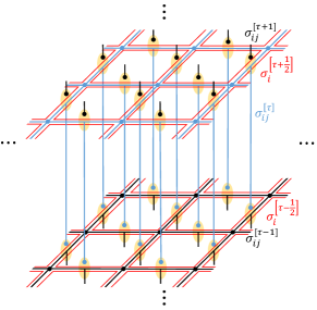
Figure 2: The entanglement between two neighbouring layers in a three-dimensional tensor network structure.

When the isotropic inter-layer and intra-layer interactions are required, we have to restrict the variational parameters as

$$\bar{J}_{A} = \bar{J}_{z}=2\tanh^{-1}h_{z}\equiv K,$$

$$\bar{J}_{x} = \bar{J}_{B}=\frac{1}{2}\log\frac{1+h_{x}^{2}}{2h_{x}}\equiv K_{\bm{p}},$$

and the number of the varying parameters are reduced. Then the obtained partition function can be simplified as

$$\mathcal{Z}_{N}=\sum_{\bm{\sigma}}\exp\left[K\sum_{\langle\bm{i}\bm{j}\rangle}\sigma_{\bm{i}\bm{j}}+K_{\bm{p}}\sum_{\bm{p}}\prod_{\langle\bm{i}\bm{j}\rangle\in\bm{p}}\sigma_{\bm{i}\bm{j}}\right],$$ (19)

where $\bm{i}=(i,\tau)$ denotes the cubic lattice sites, $\bm{p}$ are the plaquettes of the cubic lattice, and $\bm{\sigma}$ stands for the configurations of all spins $\sigma_{\bm{ij}}$ on the bonds of the cubic lattice, as displayed in Fig. 3 (a). Actually this partition function is nothing but the 3D isotropic Ising lattice gauge Higgs modelFradkin and Shenker (1979), which can also be obtained from mapping the 2D quantum Hamiltonian (13) onto a (2+1)-dimensional classical model based on imaginary time evolutionTupitsyn et al. (2010).

In the absence of the field $h_{z}$, we have $K=0$ and the obtained partition function is reduced to the 3D Ising gauge modelKogut (1979):

$$\mathcal{Z}_{N}=\sum_{\sigma}\exp\left[K_{\bm{p}}\sum_{\bm{p}}\prod_{\langle\bm{i}\bm{j}\rangle\in\bm{p}}\sigma_{\bm{i}\bm{j}}\right],$$ (20)

and a 3D Ising type of phase transition occurs at a critical value of $K_{\bm{p}}$. On the other hand, along the $h_{z}$ axis, $K_{\bm{p}}=\frac{1}{2}\log\frac{1+h_{x}^{2}}{2h_{x}}$ is extremely large and the corresponding partition function can be written

$$\mathcal{Z}_{N}=\sum_{\bm{\sigma}}\prod_{\bm{p}}\left(1+\prod_{{\langle\bm{i}\bm{j}\rangle}\in\bm{p}}\sigma_{\bm{i}\bm{j}}\right)\exp\left[K\sum_{\langle\bm{i}\bm{j}\rangle}\sigma_{\bm{i}\bm{j}}\right].$$ (21)

When new spin variables $\mu_{\bm{i}}$ are introduced on the cubic lattice sites $\bm{i}$, the spin variables $\sigma_{\bm{i}\bm{j}}$ on the bond between the sites $\bm{i}$ and $\bm{j}$ can be represented by the new variablesTrebst et al. (2007): $\sigma_{\bm{i}\bm{j}}=\mu_{\bm{i}}\mu_{\bm{j}}$, and the partition function of a 3D Ising model is thus obtained

$$\mathcal{Z}_{N}=\sum_{\mu}\exp\left[K\sum_{\langle\bm{i}\bm{j}\rangle}\mu_{\bm{i}}\mu_{\bm{i}}\right],$$ (22)

which is a 3D Ising spin model on a cubic lattice. There is a ferromagnetic-paramagnetic phase transition at a critical value of $K$.

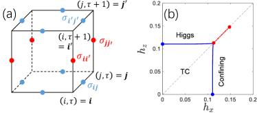
Figure 3: (a) The unit cell of the three-dimensional cubic lattice. The degrees of freedom of Ising gauge Higgs model locate on the bonds of the lattice. Each unit contains three plaquettes in average, each plaquette corresponds to a four-spin interaction term. (b) The phase diagram of the 3D isotropic Ising gauge Higgs model.

Moreover, when $h_{x}=h_{z}$, $K$ and $K_{\bm{p}}$ satisfies the self-dual condition of the Ising gauge-Higgs modelWegner (1971): $2K=-\log\tanh K_{\bm{p}}$, $2K_{\bm{p}}=-\log\tanh K$. In Fig. 3 (b), we displays the phase diagram of this 3D classical model derived from the numerical Monte Carlo calculationsJongeward et al. (1980); Tupitsyn et al. (2010); Wu et al. (2012), and the similar phase diagram has been also obtained from higher-order perturbation expansionVidal et al. (2009). Actually the phase diagram is symmetric about the self-dual line $h_{x}=h_{z}$, and the continuous phase transition between the toric code phase and Higgs (confining) belongs to the 3D Ising universality class. There is a first-order transition line along the self-dual line, but it ends at a critical point. In addition, the three transition lines just meet at a tri-critical point.

Conclusion and Outlook. -We have generalized the framework of RK wavefunctions using the TFD states. Compared with the RK wavefunctions, the TFD states contain the information of both equal and unequal time correlation functions. The partition function describing general quantum phase transitions can be extracted from the Rényi entropy of the TFD state ansatz and it is further interpreted as a 3D classical model by using the PEPS representation of the TFD state. These ideas are illustrated by mapping the general deformed toric code wavefunction into the 3D classical $\mathbb{Z}_{2}$ gauge-Higgs model. Moreover, our framework might be useful for studying the thermodynamical properties of quantum critical points. We notice the PEPS method has been used to numerically study generic quantum critical pointsCorboz et al. (2018b); Rader and Läuchli (2018b), which is beyond the RK type wavefunction with non-generic conformal quantum critical pointsArdonne et al. (2004). The static critical exponents have been accurately extracted with the finite correlation scaling methodIqbal and Schuch (2020). However, the information of dynamical exponents is not included in the PEPS. This might be improved by taking the TFD states into consideration.

Acknowledgements. -The authors are grateful to Qi Zhang for the stimulating discussions. The research is supported by the National Key Research and Development Program of MOST of China (2017YFA0302902).

References

- Verstraete et al. (2008) F. Verstraete, V. Murg, and J. Cirac, Advances in Physics 57, 143 (2008), eprint https://doi.org/10.1080/14789940801912366, URL https://doi.org/10.1080/14789940801912366.
- Schollwöck (2011) U. Schollwöck, Annals of Physics 326, 96 (2011), ISSN 0003-4916, january 2011 Special Issue, URL http://www.sciencedirect.com/science/article/pii/S0003491610001752.
- Orús (2014) R. Orús, Annals of Physics 349, 117 (2014), ISSN 0003-4916, URL http://www.sciencedirect.com/science/article/pii/S0003491614001596.
- Haegeman and Verstraete (2017) J. Haegeman and F. Verstraete, Annual Review of Condensed Matter Physics 8, 355 (2017), eprint https://doi.org/10.1146/annurev-conmatphys-031016-025507, URL https://doi.org/10.1146/annurev-conmatphys-031016-025507.
- Wolf et al. (2008) M. M. Wolf, F. Verstraete, M. B. Hastings, and J. I. Cirac, Phys. Rev. Lett. 100, 070502 (2008), URL https://link.aps.org/doi/10.1103/PhysRevLett.100.070502.
- Eisert et al. (2010) J. Eisert, M. Cramer, and M. B. Plenio, Rev. Mod. Phys. 82, 277 (2010), URL https://link.aps.org/doi/10.1103/RevModPhys.82.277.
- Verstraete and Cirac (2004) F. Verstraete and J. I. Cirac, arXiv e-prints cond-mat/0407066 (2004), eprint cond-mat/0407066.
- Jordan et al. (2008) J. Jordan, R. Orús, G. Vidal, F. Verstraete, and J. I. Cirac, Phys. Rev. Lett. 101, 250602 (2008), URL https://link.aps.org/doi/10.1103/PhysRevLett.101.250602.
- Nishino et al. (2001) T. Nishino, Y. Hieida, K. Okunishi, and N. Maeshima, Progress of Theoretical Physics 105, 409 (2001), eprint cond-mat/0011103.
- Nishio et al. (2004) Y. Nishio, N. Maeshima, A. Gendiar, and T. Nishino, arXiv e-prints cond-mat/0401115 (2004), eprint cond-mat/0401115.
- Schuch et al. (2012) N. Schuch, D. Poilblanc, J. I. Cirac, and D. Pérez-García, Phys. Rev. B 86, 115108 (2012), URL https://link.aps.org/doi/10.1103/PhysRevB.86.115108.
- Schuch et al. (2013) N. Schuch, D. Poilblanc, J. I. Cirac, and D. Pérez-García, Phys. Rev. Lett. 111, 090501 (2013), URL https://link.aps.org/doi/10.1103/PhysRevLett.111.090501.
- Rader and Läuchli (2018a) M. Rader and A. M. Läuchli, Phys. Rev. X 8, 031030 (2018a), URL https://link.aps.org/doi/10.1103/PhysRevX.8.031030.
- Corboz et al. (2018a) P. Corboz, P. Czarnik, G. Kapteijns, and L. Tagliacozzo, Phys. Rev. X 8, 031031 (2018a), URL https://link.aps.org/doi/10.1103/PhysRevX.8.031031.
- Isakov et al. (2011) S. V. Isakov, P. Fendley, A. W. W. Ludwig, S. Trebst, and M. Troyer, Phys. Rev. B 83, 125114 (2011), URL https://link.aps.org/doi/10.1103/PhysRevB.83.125114.
- Haegeman et al. (2015) J. Haegeman, K. Van Acoleyen, N. Schuch, J. I. Cirac, and F. Verstraete, Phys. Rev. X 5, 011024 (2015), URL https://link.aps.org/doi/10.1103/PhysRevX.5.011024.
- Zhu and Zhang (2019) G.-Y. Zhu and G.-M. Zhang, Phys. Rev. Lett. 122, 176401 (2019), URL https://link.aps.org/doi/10.1103/PhysRevLett.122.176401.
- Xu et al. (2020) W.-T. Xu, Q. Zhang, and G.-M. Zhang, Phys. Rev. Lett. 124, 130603 (2020), URL https://link.aps.org/doi/10.1103/PhysRevLett.124.130603.
- Ardonne et al. (2004) E. Ardonne, P. Fendley, and E. Fradkin, Annals of Physics 310, 493 (2004), ISSN 00034916, URL http://linkinghub.elsevier.com/retrieve/pii/S0003491604000247.
- Castelnovo et al. (2005) C. Castelnovo, C. Chamon, C. Mudry, and P. Pujol, Annals of Physics 318, 316 (2005), ISSN 0003-4916, URL http://www.sciencedirect.com/science/article/pii/S0003491605000096.
- Verstraete et al. (2006) F. Verstraete, M. M. Wolf, D. Perez-Garcia, and J. I. Cirac, Phys. Rev. Lett. 96, 220601 (2006), URL https://link.aps.org/doi/10.1103/PhysRevLett.96.220601.
- Takahashi and Umezawa (1996) Y. Takahashi and H. Umezawa, International Journal of Modern Physics B 10, 1755 (1996), eprint https://doi.org/10.1142/S0217979296000817, URL https://doi.org/10.1142/S0217979296000817.
- Kitaev (2003) A. Y. Kitaev, Annals of Physics 303, 2 (2003), ISSN 0003-4916, URL http://www.sciencedirect.com/science/article/pii/S0003491602000180.
- Vidal et al. (2009) J. Vidal, S. Dusuel, and K. P. Schmidt, Phys. Rev. B 79, 033109 (2009), URL https://link.aps.org/doi/10.1103/PhysRevB.79.033109.
- Tupitsyn et al. (2010) I. S. Tupitsyn, A. Kitaev, N. V. Prokof’ev, and P. C. E. Stamp, Phys. Rev. B 82, 085114 (2010), URL https://link.aps.org/doi/10.1103/PhysRevB.82.085114.
- Fradkin and Shenker (1979) E. Fradkin and S. H. Shenker, Phys. Rev. D 19, 3682 (1979), URL https://link.aps.org/doi/10.1103/PhysRevD.19.3682.
- Jongeward et al. (1980) G. A. Jongeward, J. D. Stack, and C. Jayaprakash, Phys. Rev. D 21, 3360 (1980), URL https://link.aps.org/doi/10.1103/PhysRevD.21.3360.
- Molnar et al. (2015) A. Molnar, N. Schuch, F. Verstraete, and J. I. Cirac, Phys. Rev. B 91, 045138 (2015), URL https://link.aps.org/doi/10.1103/PhysRevB.91.045138.
- Vanderstraeten et al. (2017) L. Vanderstraeten, M. Mariën, J. Haegeman, N. Schuch, J. Vidal, and F. Verstraete, Phys. Rev. Lett. 119, 070401 (2017), URL https://link.aps.org/doi/10.1103/PhysRevLett.119.070401.
- Schotte et al. (2019) A. Schotte, J. Carrasco, B. Vanhecke, L. Vanderstraeten, J. Haegeman, F. Verstraete, and J. Vidal, Phys. Rev. B 100, 245125 (2019), URL https://link.aps.org/doi/10.1103/PhysRevB.100.245125.
- Kogut (1979) J. B. Kogut, Rev. Mod. Phys. 51, 659 (1979), URL https://link.aps.org/doi/10.1103/RevModPhys.51.659.
- Trebst et al. (2007) S. Trebst, P. Werner, M. Troyer, K. Shtengel, and C. Nayak, Phys. Rev. Lett. 98, 070602 (2007), URL https://link.aps.org/doi/10.1103/PhysRevLett.98.070602.
- Wegner (1971) F. J. Wegner, Journal of Mathematical Physics 12, 2259 (1971), ISSN 0022-2488, URL https://aip.scitation.org/doi/10.1063/1.1665530.
- Wu et al. (2012) F. Wu, Y. Deng, and N. Prokof’ev, Phys. Rev. B 85, 195104 (2012), URL https://link.aps.org/doi/10.1103/PhysRevB.85.195104.
- Corboz et al. (2018b) P. Corboz, P. Czarnik, G. Kapteijns, and L. Tagliacozzo, Phys. Rev. X 8, 031031 (2018b), URL https://link.aps.org/doi/10.1103/PhysRevX.8.031031.
- Rader and Läuchli (2018b) M. Rader and A. M. Läuchli, Phys. Rev. X 8, 031030 (2018b), URL https://link.aps.org/doi/10.1103/PhysRevX.8.031030.
- Iqbal and Schuch (2020) M. Iqbal and N. Schuch, arXiv e-prints arXiv:2011.06611 (2020), eprint 2011.06611.