Probing the dynamics of
chiral $SU(N)$ gauge theories
via generalized anomalies

Abstract

We study symmetries and dynamics of chiral $SU(N)$ gauge theories with matter Weyl fermions in a two-index symmetric ($\psi$) or anti-symmetric tensor ($\chi$) representation, together with $N\pm 4+p$ fermions in the anti-fundamental ($\eta$) and $p$ fermions in the fundamental ($\xi$) representations. They are known as the Bars-Yankielowicz (the former) and the generalized Georgi-Glashow models (the latter). The conventional ’t Hooft anomaly matching algorithm is known to allow a confining, chirally symmetric vacuum in all these models, with a simple set of massless baryonlike composite fermions describing the infrared physics.

We analyzed recently one of these models ($\psi\eta$ model), by applying the ideas of generalized symmetries and the consequent, stronger constraints involving certain mixed anomalies, finding that the confining, chirally symmetric, vacuum is actually inconsistent.

In the present paper this result is extended to a wider class of the Bars-Yankielowicz and the generalized Georgi-Glashow models. It is shown that for all these models with $N$ and $p$ both even, at least, the generalized anomaly matching requirement forbids the persistence of the full chiral symmetries in the infrared if the system confines. The most natural and consistent possibility is that some bifermion condensates form, breaking the color gauge symmetry dynamically, together with part of the global symmetry.

1 Introduction

A few steps have been taken recently [1, 2] to go beyond the conventional ’t Hooft anomaly matching analysis in understanding the infrared dynamics of chiral gauge theories. The standard anomaly matching constraints and other generally accepted ideas, are usually not sufficient to pinpoint what happens in the infrared, where the system gets strongly coupled and perturbation theory has a limited power in predicting the phase and global symmetry realization patterns.

The tools which allow these new results come from the idea of the generalized symmetries, of gauging some 1-form discrete center symmetries and studying the consequences of mixed-’t Hooft-anomaly-matching conditions [3]-​​[16]. Most concrete applications of these new techniques so far refer to vectorlike gauge theories, such as pure $SU(N)$ Yang-Mills, or adjoint QCD, where there is an exact center symmetry (${\mathbbm{Z}}_{N}$ for $SU(N)$ theories), or QCD where the color center symmetry can be combined with $U(1)_{V}$ to give a color-flavor locked 1-form center symmetry. In these, vectorlike, gauge theories, the results from the new approach can be corroborated by the extensive literature, based on some general theorems [17, 18], on lattice simulations [19]-​​[22], on the effective Lagrangians [23]-​​[26], on ’t Hooft anomaly analysis [27], on the powerful exact results in ${\cal N}=2$ supersymmetrie theories [28, 29], or on some other theoretical ideas such as the space compactification combined with semi-classical analyses [30]-​​[33].

Most of these theoretical tools are however unavailable for the study of strongly-coupled chiral gauge theories, except for some general wisdom, the large-$N$ approximation, and the ’t Hooft anomaly considerations. Together, they offer significant, but not very stringent, information on the infrared dynamics, phases, and symmetry realization (see [34]-​​[47]). Such a situation is doubtlessly limiting our capability of utilizing chiral gauge theories in the context of realistic model building beyond the standard model, e.g., with composite fermions, with composite Higgs bosons, or with dynamical composite models for dark matter, and so on.

It was these considerations that recently motivated the present authors to apply some of the new concepts and techniques to chiral gauge theories, to see if new insights in the physics of these theories can be gained by doing so [1, 2]. In particular, in [2], a simple class of $SU(N)$ gauge theories with Weyl fermions

$$\psi^{ij}\,,\quad\eta_{i}^{A}\,,\qquad{\footnotesize i,j=1,\ldots,N\;,\quad A=1,\ldots,N+4}\;,$$ (1.1)

in the direct-sum representation

$$\yng(2)\oplus(N+4)\,{\bar{{\yng(1)}}}\;,$$ (1.2)

(“$\psi\eta$ model”) was studied. For even $N$ the (nonanomalous) symmetry of the system is

$$SU(N)\times G_{\mathrm{f}}\;,\qquad G_{\mathrm{f}}=\frac{SU(N+4)\times U(1)_{\psi\eta}\times(\mathbb{Z}_{2})_{F}}{\mathbb{Z}_{N}\times\mathbb{Z}_{N+4}}\;,$$ (1.3)

where $U(1)_{\psi\eta}$ is the anomaly-free combination of $U(1)_{\psi}$ and $U(1)_{\eta}$, and $(\mathbb{Z}_{2})_{F}$ is the fermion parity, $\psi,\eta\to-\psi,-\eta$.

In spite of the presence of fermions in the fundamental representation of $SU(N)$ the system turns out to possess, classically, an exact discrete ${\mathbbm{Z}}_{N}$ center 1-form symmetry ,

$${\mathbbm{Z}}_{N}=SU(N)\cap\{U(1)_{\psi\eta}\times(\mathbb{Z}_{2})_{F}\}\;.$$ (1.4)

Indeed, the gauge transformation with $\mathrm{e}^{\frac{2\pi\mathrm{i}}{N}}\in\mathbb{Z}_{N}\subset SU(N)$,

$$\psi\to\mathrm{e}^{\frac{4\pi\mathrm{i}}{N}}\psi\;,\;\qquad\eta\to\mathrm{e}^{-\frac{2\pi\mathrm{i}}{N}}\eta\;,$$ (1.5)

can be undone by the following $(\mathbb{Z}_{2})_{F}\times U(1)_{\psi\eta}$ transformation:

$$\psi\to(-1)\,\mathrm{e}^{\mathrm{i}{N+4\over 2}{2\pi\over N}}\psi=\mathrm{e}^{-\mathrm{i}{N\over 2}{2\pi\over N}}\,\mathrm{e}^{\mathrm{i}{N+4\over 2}{2\pi\over N}}\psi\;,\qquad\eta\to(-1)\,\mathrm{e}^{-\mathrm{i}{N+2\over 2}{2\pi\over N}}\eta=\mathrm{e}^{\mathrm{i}{N\over 2}{2\pi\over N}}\,\mathrm{e}^{-\mathrm{i}{N+2\over 2}{2\pi\over N}}\eta\;.$$ (1.6)

Note that the odd elements of $\mathbb{Z}_{N}$ belong to the disconnected component of $U(1)_{\psi\eta}\times(\mathbb{Z}_{2})_{F}$ while the even elements belong to the identity component.

The central idea is now to “gauge” this discrete, color-flavor locked 1-form $\mathbb{Z}_{N}$ symmetry. Remember that the unfamiliar-sounding expression of gauging a discrete symmetry means simply that field configurations related by it are identified and the redundancy eliminated. This implies redefinition of the path-integral sum over the gauge field configurations appropriately. By applying this to the 1-form ${\mathbbm{Z}}_{N}$ of an $SU(N)$ gauge theory, one arrives at an $\frac{SU(N)}{{\mathbbm{Z}}_{N}}$ gauge system, with consequent $\frac{1}{N}$ fractional instanton numbers. Concretely, this can be done by introducing the 2-form gauge fields $\big{(}B_{\mathrm{c}}^{(2)}$, $B_{\mathrm{c}}^{(1)}\big{)}$,

$$NB_{\mathrm{c}}^{(2)}=dB_{\mathrm{c}}^{(1)}\;,$$ (1.7)

and coupling to them the $SU(N)$ gauge fields $a$ and $U(1)_{\psi\eta}\times(\mathbb{Z}_{2})_{F}$ gauge fields, $A$ and $A_{2}^{(1)}$, appropriately. As for the $SU(N)$ gauge field $a$, this can be achieved by embedding it into a $U(N)$ gauge field $\widetilde{a}$ as

$$\widetilde{a}=a+{1\over N}B^{(1)}_{\mathrm{c}},$$ (1.8)

and requiring the whole system to be invariant under the 1-form gauge transformation,

$$B_{\mathrm{c}}^{(2)} \to B_{\mathrm{c}}^{(2)}+\mathrm{d}\lambda_{\mathrm{c}}\;,\qquad B_{\mathrm{c}}^{(1)}\to B_{\mathrm{c}}^{(1)}+N\lambda_{\mathrm{c}}\;,$$

$$\widetilde{a} \to\widetilde{a}+\lambda_{\mathrm{c}}\;.$$ (1.9)

As the ${\mathbbm{Z}}_{N}$ is a color-flavor locked symmetry, Eq. (1.4), the $U(1)_{\psi\eta}$ and $(\mathbb{Z}_{2})_{F}$ gauge fields must also be transformed simultaneously:

$$A\to A-\lambda_{\mathrm{c}}\;,\qquad A_{2}^{(1)}\to A_{2}^{(1)}+{N\over 2}\lambda_{\mathrm{c}}\;.\;$$ (1.10)

The relation (1.7) indicates that one has now an $\frac{SU(N)}{{\mathbbm{Z}}_{N}}$ connection rather than $SU(N)$. It implies that there are nontrivial ’t Hooft fluxes carried by the gauge fields

$$\frac{1}{2\pi}\int_{\Sigma_{2}}B_{\mathrm{c}}^{(2)}=\frac{n_{1}}{N}\;,\qquad n_{1}\in{\mathbbm{Z}}_{N}\;,$$ (1.11)

in a closed two-dimensionl subspace, ${\Sigma_{2}}$. On topologically nontrivial four dimensional spacetime of Euclidean signature containing such subspaces one has then

$$\frac{1}{8\pi^{2}}\int_{\Sigma_{4}}(B_{\mathrm{c}}^{(2)})^{2}=\frac{n}{N^{2}}\;,$$ (1.12)

where $n\in{\mathbbm{Z}}_{N}$.

The fermion kinetic term with the background gauge field is obtained by the minimal coupling procedure as

$$\overline{\psi}\gamma^{\mu}\Big{(}\partial+\mathcal{R}_{\mathrm{S}}(\widetilde{a})+{N+4\over 2}A+A_{2}\Big{)}_{\mu}P_{\mathrm{L}}\psi+\;$$

$$\overline{\eta}\gamma^{\mu}\Big{(}\partial+\mathcal{R}_{\mathrm{F}^{*}}(\widetilde{a})-{N+2\over 2}A-A_{2}\Big{)}_{\mu}P_{\mathrm{L}}\eta\;,$$ (1.13)

with the obvious notation. We compute the anomalies by applying the Stora-Zumino descent procedure starting with a $6D$ anomaly functional

$${\cal T}_{1} = {1\over 24\pi^{2}}\,{\mathrm{tr}}_{\mathcal{R}_{\mathrm{S}}}\left[\mathcal{R}_{\mathrm{S}}\big{(}F(\tilde{a})-B^{(2)}_{\mathrm{c}}\big{)}+{N+4\over 2}\Big{(}{\mathrm{d}}A+B^{(2)}_{\mathrm{c}}\Big{)}+\Big{(}\mathrm{d}A_{2}^{(1)}-{N\over 2}B^{(2)}_{\mathrm{c}}\Big{)}\right]^{3}\;,$$

$${\cal T}_{2} = {1\over 24\pi^{2}}\,{\mathrm{tr}}_{\mathcal{R}_{\mathrm{F}}^{*}}\left[-\big{(}F(\widetilde{a})-B^{(2)}_{\mathrm{c}}\big{)}-{N+2\over 2}\Big{(}{\mathrm{d}}A+B^{(2)}_{\mathrm{c}}\Big{)}-\Big{(}\mathrm{d}A_{2}^{(1)}-{N\over 2}B^{(2)}_{\mathrm{c}}\Big{)}\right]^{3}\;.$$

The rest of the procedure for computing the $(\mathbb{Z}_{2})_{F}$ anomaly is standard: (i) one first integrates to get the $5D$ boundary action containing $A_{2}^{(1)}$ (WZW action); (ii) the variations of the form

$$\delta A_{2}^{(1)}=\frac{1}{2}\partial\delta A_{2}^{(0)}\;,\qquad\delta A_{2}^{(0)}=\pm 2\pi\;,$$ (1.15)

leads to, via the anomaly-in-flow, the seeked-for anomaly in the $4D$ theory. The result is

$$\delta S=-N^{2}\,{1\over 8\pi^{2}}\int_{\Sigma^{4}}(B^{(2)}_{\mathrm{c}})^{2}\,\frac{1}{2}\delta A_{2}^{(0)}=-N^{2}\times\frac{\mathbbm{Z}}{N^{2}}\,({\pm\pi})=\pm\pi\times{\mathbbm{Z}}\;:$$ (1.16)

the partition function changes sign, under $\psi,\eta\to-\psi,-\eta$, that is, there is a $(\mathbb{Z}_{2})_{F}$ anomaly.

As the $({\mathbbm{Z}}_{2})_{F}-[{\mathbbm{Z}}_{N}]^{2}$ mixed anomaly is obviously absent in the IR, we conclude that the confining chirally symmetric vacuum, in which conventional ’t Hooft anomalies are saturated in the infrared by massless composite “baryons”

$${\cal B}^{AB}=\psi^{ij}\eta_{i}^{A}\eta_{j}^{B}\;,\qquad A,B=1,\ldots,N+4\;,$$ (1.17)

(antisymmetric in $A\leftrightarrow B$), is not the correct vacuum of the system. As shown in [2], the dynamical Higgs vacuum, characterized by bifermion condensates,

$$\langle\psi^{ij}\eta_{i}^{B}\rangle=\,c\,\Lambda^{3}\delta^{jB}\neq 0\;,\qquad j,B=1,\dots N\;,\qquad c\sim O(1)$$ (1.18)

is instead found to be fully consistent.

Several subtle features of the calculation and in the interpretation of the results are discussed carefully in [2].

The purpose of the present work is to investigate if the result found in the $\psi\eta$ model extends naturally to a wider class of the so-called Bars-Yankielowicz and the generalized Georgi-Glashow models. The gauge group is taken to be $SU(N)$, and the matter fermion content is ($p$ is a natural number)

$$\yng(2)\oplus(N+4+p)\,{\bar{{\yng(1)}}}\;\oplus p\,{{{\yng(1)}}}\;$$ (1.19)

for the former (let us call them $\{{\cal S},N,p\}$ models), and

$$\yng(1,1)\oplus(N-4+p)\,{\bar{{\yng(1)}}}\;\oplus p\,{{{\yng(1)}}}\;$$ (1.20)

for the latter ($\{{\cal A},N,p\}$ models). We will find that for all $N$ and $p$, both even, the system possesses a $(\mathbb{Z}_{2})_{F}$ symmetry, which is nonanomalous, i.e., respected by standard instantons. Also, these models all enjoy a “color-flavor locked” ${\mathbbm{Z}}_{N}$ center symmetry, in spite of the presence of fermions in the fundamental (or anti-fundamental) representation. It is thus possible to gauge this center symmetry and study if, by doing so, the $(\mathbb{Z}_{2})_{F}$ symmetry becomes anomalous, as happened in the $\{{\cal S},N,0\}$ model.

The paper is organized as follows. In Sec. 2 we discuss the conventional ’t Hooft-anomaly-matching analysis in all these models. A good part of this section is a review of [34]-[40], but there are some new results, especially concerning the Higgs phase, which we need later. As the global symmetry group is relatively large, the fact that one can find a set of gauge-invariant composite fermions which satisfy all the anomaly-matching equations at all, assuming the system to confine, is quite remarkable. Also, in all these models we find an alternative phase, also consistent with the anomaly matching criterion, characterized by certain bifermion condensates breaking color dynamically (dynamical Higgs phase) accompanied by a partial breaking of the global symmetry.

In the conventional ’t Hooft anomaly matching equations, only the perturbative (local) aspect of the flavor symmetry group matters, though nonperturbative (instanton) effects of the strong $SU(N)$ gauge interactions are taken into account. In Sec. 3, the symmetry of these models is re-analyzed more carefully, taking into account the global properties (e.g., the connectedness).

In Sec. 4.2 we calculate and find a mixed anomaly of the type, $({\mathbbm{Z}}_{2})_{F}-[{\mathbbm{Z}}_{N}]^{2}$, in all models with $N$ and $p$ both even, whereas such an anomaly is absent in the infrared (IR) in a confining vacuum with full global symmetry - one of the candidate vacua allowed by the conventional anomaly matching argument. Consistency implies that these vacua cannot be realized dynamically in the infrared, in all $\{{\cal S},N,p\}$ and $\{{\cal A},N,p\}$ models, with $N$ and $p$ are both even.

We summarize and discuss our results in Sec. 5.

2 Theories and possible phases

2.1 $\{{\cal S},N,p\}$ models

The first class of theories is the $\psi\eta$ model with additional $p$ pairs of fundamental and anti-fundamental fermions. Namely, the model is an $SU(N)$ gauge theory with Weyl fermions

$$\psi^{ij}\,,\quad\eta_{i}^{A}\,\,,\quad\xi^{i,a}$$ (2.1)

in the direct-sum representation

$$\yng(2)\oplus(N+4+p)\,{\bar{{\yng(1)}}}\;\oplus p\,{{{\yng(1)}}}\;.$$ (2.2)

The indices run as

$$\footnotesize i,j=1,\ldots,N\;,\quad A=1,\ldots,N+4+p\;,\quad a=1,\ldots,p\;.$$ (2.3)

These theories (the Bars-Yankielowicz models) will be denoted as $\{{\cal S},N,p\}$ below. The $\psi\eta$ model corresponds to $\{{\cal S},N,0\}$. The first coefficient of the beta function is

$$b_{0}=11N-(N+2)-(N+4+2p)=9N-6-2p\;,$$ (2.4)

and $p$ is limited by $\frac{9}{2}N-3$ before asymptotic freedom (AF) is lost. In the limit $N$ fixed and $p\to\infty$ we recover ordinary QCD with $p$ flavors, although this is outside the regime of AF. The classical symmetry group is

$$SU(N)_{\mathrm{c}}\times U(1)_{\psi}\times U(N+4+p)_{\eta}\times U(p)_{\xi}\;.$$ (2.5)

We discuss for the moment only $0$-form symmetries, leaving a more detailed discussion of the symmetry group to Sec. 3. Anomaly breaks the symmetry group (2.5) to

$$p=0:\quad SU(N)_{\mathrm{c}}\times SU(N+4)_{\eta}\times U(1)_{\psi\eta}\;,$$

$$p=1:\quad SU(N)_{\mathrm{c}}\times SU(N+5)_{\eta}\times U(1)_{\psi\eta}\times U(1)_{\psi\xi}\;,$$

$$p>1:\quad SU(N)_{\mathrm{c}}\times SU(N+4+p)_{\eta}\times SU(p)_{\xi}\times U(1)_{\psi\eta}\times U(1)_{\psi\xi}\;,$$ (2.6)

where the anomaly-free combination of $U(1)_{\psi}$ and $U(1)_{\eta}$ is

$$U(1)_{\psi\eta}:\qquad\psi\to\mathrm{e}^{\mathrm{i}(N+4+p)\alpha}\psi\;,\quad\eta\to\mathrm{e}^{-\mathrm{i}(N+2)\alpha}\eta\;,$$ (2.7)

with $\alpha\in\mathbbm{R}$, and the anomaly-free combination of $U(1)_{\psi}$ and $U(1)_{\xi}$ is

$$U(1)_{\psi\xi}:\qquad\psi\to\mathrm{e}^{\mathrm{i}p\beta}\psi\;,\quad\xi\to\mathrm{e}^{-\mathrm{i}(N+2)\beta}\xi\;,$$ (2.8)

with $\beta\in\mathbbm{R}$. The choice of the two unbroken $U(1)$’s is somehow arbritrary, for example also $U(1)_{\eta\xi}$

$$U(1)_{\eta\xi}:\qquad\eta\to\mathrm{e}^{\mathrm{i}p\gamma}\eta\;,\quad\xi\to\mathrm{e}^{-\mathrm{i}(N+4+p)\gamma}\xi\;,$$ (2.9)

with $\gamma\in\mathbbm{R}$ could be chosen as a generator. In Table 1 we summarize the fields and how they transform under the symmetry group.

	$SU(N)_{\rm c}$	$SU(N+4+p)$	$SU(p)$	${U}(1)_{\psi\eta}$	${U}(1)_{\psi\xi}$
$\psi$	${\yng(2)}$	$\frac{N(N+1)}{2}\cdot(\cdot)$	$\frac{N(N+1)}{2}\cdot(\cdot)$	$N+4+p$	$p$
$\eta$	$(N+4+p)\cdot{\bar{\yng(1)}}$	$N\cdot{\yng(1)}$	$N(N+4+p)\,\cdot(\cdot)$	$-(N+2)$	$0$
$\xi$	$p\cdot{{\yng(1)}}$	$Np\,\cdot(\cdot)$	$N\cdot{{\yng(1)}}$	$0$	$-(N+2)$

Table 1: The multiplicity, charges and the representation are shown for each set of fermions in the $\{{\cal S},N,p\}$ model. $(\cdot)$ stands for a singlet representation.

There are also discrete unbroken symmetries of the three $U(1)$’s: $({\mathbbm{Z}}_{N+2})_{\psi}$, $({\mathbbm{Z}}_{N+4+p})_{\eta}$ and $({\mathbbm{Z}}_{p})_{\xi}$. The relation between these discrete symmetries and the continuous non-anomalos group $U(1)_{\psi\eta}\times U(1)_{\psi\xi}$ will be discussed in Sec. 3.

2.2 $\{{\cal A},N,p\}$ models

The second class of models we are interested are $SU(N)$ gauge theories with Weyl fermions

$$\chi^{ij}\,,\quad\eta_{i}^{A}\,\,,\quad\xi^{i,a}$$ (2.10)

in the direct-sum representation

$$\yng(1,1)\oplus(N-4+p)\,{\bar{{\yng(1)}}}\;\oplus p\,{{{\yng(1)}}}\;.$$ (2.11)

The indices run as

$$\footnotesize i,j=1,\ldots,N\;,\quad A=1,\ldots,N-4+p\;,\quad a=1,\ldots,p\;.$$ (2.12)

These (the generalized Georgi-Glashow) models will be indicated as $\{{\cal A},N,p\}$. The first coefficient of the beta function is

$$b_{0}=11N-(N-2)-(N-4+2p)=9N+6-2p\;.$$ (2.13)

Here $p$ will be assumed to be less than $\frac{9}{2}N+3$ so as to maintain AF. The symmetry group is

$$SU(N)_{\mathrm{c}}\times U(1)_{\chi}\times U(N-4+p)_{\eta}\times U(p)_{\xi}\;.$$ (2.14)

Anomaly breaks this group to

$$p=0:\quad SU(N)_{\mathrm{c}}\times SU(N-4)_{\eta}\times U(1)_{\chi\eta}\;,$$

$$p=1:\quad SU(N)_{\mathrm{c}}\times SU(N-3)_{\eta}\times U(1)_{\chi\eta}\times U(1)_{\chi\xi}\;,$$

$$p>1:\quad SU(N)_{\mathrm{c}}\times SU(N-4+p)_{\eta}\times SU(p)_{\xi}\times U(1)_{\chi\eta}\times U(1)_{\chi\xi}\;,$$ (2.15)

where the anomaly-free combination of $U(1)_{\chi}$ and $U(1)_{\eta}$ is

$$U(1)_{\chi\eta}:\ \chi\to\mathrm{e}^{\mathrm{i}(N-4+p)\alpha}\chi\;,\qquad\eta\to\mathrm{e}^{-\mathrm{i}(N-2)\alpha}\eta\;,$$ (2.16)

and the anomaly-free combination of $U(1)_{\psi}$ and $U(1)_{\xi}$ is

$$U(1)_{\chi\xi}:\ \chi\to\mathrm{e}^{\mathrm{i}p\beta}\chi\;,\qquad\xi\to\mathrm{e}^{-\mathrm{i}(N-2)\beta}\xi\;.$$ (2.17)

Another possible anomaly-free combination is $U(1)_{\eta\xi}$:

$$U(1)_{\eta\xi}:\ \eta\to\mathrm{e}^{\mathrm{i}p\gamma}\eta\;,\qquad\xi\to\mathrm{e}^{-\mathrm{i}(N-4+p)\gamma}\xi\;.$$ (2.18)

In Table 2 we summarize the fields and how they transform under the symmetry group.

	$SU(N)_{\rm c}$	$SU(N-4+p)$	$SU(p)$	${U}(1)_{\chi\eta}$	${U}(1)_{\chi\xi}$
$\chi$	${\yng(1,1)}$	$\frac{N(N-1)}{2}\cdot(\cdot)$	$\frac{N(N-1)}{2}\cdot(\cdot)$	$N-4+p$	$p$
$\eta$	$(N-4+p)\cdot{\bar{\yng(1)}}$	$N\cdot{\yng(1)}$	$N(N-4+p)\,\cdot(\cdot)$	$-(N-2)$	$0$
$\xi$	$p\cdot{{\yng(1)}}$	$Np\,\cdot(\cdot)$	$N\cdot{{\yng(1)}}$	$0$	$-(N-2)$

Table 2: The multiplicity, charges and the representation are shown for each set of fermions in the $\{{\cal A},N,p\}$ model.

There are also discrete unbroken symmetries: $({\mathbbm{Z}}_{N-2})_{\psi}$, $({\mathbbm{Z}}_{N-4+p})_{\eta}$ and $({\mathbbm{Z}}_{p})_{\xi}$.

2.3 Confining phase with unbroken global symmetries

The standard ’t Hooft anomaly matching conditions were found to allow a chirally symmetric, confining vacuum in the model first proposed in [35]. Let us assume that no condensates form, the system confines, and the flavor symmetry is unbroken.

2.3.1 $\{{\cal S},N,p\}$ models

The candidate massless composite fermions for the $\{{\cal S},N,p\}$ models are the left-handed gauge-invariant fields:

$${({\cal B}_{1})}^{[AB]}=\psi^{ij}\eta_{i}^{A}\eta_{j}^{B}\;,\qquad{({\cal B}_{2})}^{a}_{A}=\bar{\psi}_{ij}\bar{\eta}^{i}_{A}\xi^{j,a}\;,\qquad{({\cal B}_{3})}_{\{ab\}}=\psi^{ij}{\bar{\xi}}_{i,a}{\bar{\xi}}_{j,b}\;,$$ (2.19)

the first is anti-symmetric in $A\leftrightarrow B$ and the third is symmetric in $a\leftrightarrow b$; their charges are given in Table 3. Writing explicitly also the spin indices they are

$${({\cal B}_{1})}^{AB,\alpha}=\frac{1}{2}\epsilon_{\beta\gamma}\psi^{ij,\beta}\eta_{i}^{A,\gamma}\eta_{j}^{B,\alpha}+\frac{1}{2}\epsilon_{\beta\gamma}\psi^{ij,\beta}\eta_{i}^{A,\alpha}\eta_{j}^{B,\gamma}\;,$$

$${({\cal B}_{2})}^{a,\alpha}_{A}=\epsilon_{\dot{\alpha}\dot{\beta}}\bar{\psi}_{ij}^{\dot{\alpha}}\bar{\eta}^{i,\dot{\beta}}_{A}\xi^{j,a,\alpha}\;,\qquad{({\cal B}_{3})}_{ab}^{\alpha}=\epsilon_{\dot{\beta}\dot{\gamma}}\psi^{ij,\alpha}{\bar{\xi}}_{i,a}^{\dot{\beta}}{\bar{\xi}}_{j,b}^{\dot{\gamma}}\;:$$ (2.20)

all transforming under the $\{\tfrac{1}{2},0\}$ representation of the Lorentz group.

	$SU(N)_{\rm c}$	$SU(N+4+p)$	$SU(p)$	${U}(1)_{\psi\eta}$	${U}(1)_{\psi\xi}$
${{\cal B}_{1}}$	$\frac{(N+4+p)(N+3+p)}{2}\cdot(\cdot)$	${\yng(1,1)}$	$\frac{(N+4+p)(N+3+p)}{2}\cdot(\cdot)$	$-N+p$	$p$
${{\cal B}_{2}}$	$(N+4+p)p\cdot(\cdot)$	$p\cdot\bar{\yng(1)}$	$(N+4+p)\cdot{\yng(1)}$	$-(p+2)$	$-(N+p+2)$
${{\cal B}_{3}}$	$\frac{p(p+1)}{2}\cdot(\cdot)$	$\frac{p(p+1)}{2}\cdot(\cdot)$	$\bar{\yng(2)}$	$N+4+p$	$2N+4+p$

Table 3: Chirally symmetric phase of the $\{{\cal S},N,p\}$ model.

Table 4 summarizes the anomaly matching checks, via comparison between Table 1 and Table 3.

	UV	IR
$SU(N+4+p)^{3}$	$N$	$N+p-p$
$SU(p)^{3}$	$N$	$N+4+p-(p+4)$
$SU(N+4+p)^{2}-{U}(1)_{\psi\eta}$	$-N(N+2)$	$-(N+2+p)(N-p)-p(p+2)$
$SU(N+4+p)^{2}-{U}(1)_{\psi\xi}$	$0$	$(N+2+p)p-p(N+p+2)$
$SU(p)^{2}-{U}(1)_{\psi\eta}$	$0$	$-(N+4+p)(p+2)+(p+2)(N+p+4)$
$SU(p)^{2}-{U}(1)_{\psi\xi}$	$-N(N+2)$	$-(N+4+p)(N+p+2)+(p+2)(2N+p+4)$
${U}(1)_{\psi\eta}^{3}$	$\frac{N(N+1)}{2}(N+4+p)^{3}-N(N+4+p)(N+2)^{3}$	$-\frac{(N+4+p)(N+3+p)}{2}(N-p)^{3}-(N+4+p)p(p+2)^{3}+$
		$+\frac{p(p+1)}{2}(N+4+p)^{3}$
${U}(1)_{\psi\xi}^{3}$	$\frac{N(N+1)}{2}p^{3}-Np(N+2)^{3}$	$\frac{(N+4+p)(N+3+p)}{2}p^{3}-(N+4+p)p(N+p+2)^{3}+$
		$\ +\frac{p(p+1)}{2}(2N+4+p)^{3}$
${\rm Grav}^{2}-{U}(1)_{\psi\eta}$	$\frac{N(N+1)}{2}(N+4+p)-N(N+4+p)(N+2)$	$-\frac{(N+4+p)(N+3+p)}{2}(N-p)-(N+4+p)p(p+2)+$
		$+\frac{p(p+1)}{2}(N+4+p)$
${\rm Grav}^{2}-{U}(1)_{\psi\xi}$	$\frac{N(N+1)}{2}p-Np(N+2)$	$\frac{(N+4+p)(N+3+p)}{2}p-(N+4+p)p(N+p+2)+$
		$\ +\frac{p(p+1)}{2}(2N+4+p)$
$SU(N+4+p)^{2}-({\mathbbm{Z}}_{N+2})_{\psi}$	$0$	$N+2+p-p=0\ {\rm mod}\ N+2$
$SU(p)^{2}-({\mathbbm{Z}}_{N+2})_{\psi}$	$0$	$-(N+4+p)+p+2=0\ {\rm mod}\ N+2$
${\rm Grav}^{2}-({\mathbbm{Z}}_{N+2})_{\psi}$	$1$	$1-1+1$

Table 4: Anomaly matching checks for the IR chiral symmetric phase of the $\{{\cal S},N,p\}$ model. For $N$ odd, the last three equalities are consequences of other equations.

2.3.2 $\{{\cal A},N,p\}$ models

The candidate massless composite fermions for the $\{{\cal A},N,p\}$ model are:

$${({\cal B}_{1})}^{\{AB\}}=\chi^{ij}\eta_{i}^{A}\eta_{j}^{B}\;,\qquad{({\cal B}_{2})}^{a}_{A}=\bar{\chi}_{ij}\bar{\eta}^{i}_{A}\xi^{j,a}\;,\qquad{({\cal B}_{3})}_{[ab]}=\chi^{ij}{\bar{\xi}}_{i,a}{\bar{\xi}}_{j,b}\;,$$ (2.21)

the first symmetric in $A\leftrightarrow B$ and the third anti-symmetric in $a\leftrightarrow b$. Writing the spin indices explicitly they are:

$${({\cal B}_{1})}^{AB,\alpha}=\frac{1}{2}\epsilon_{\beta\gamma}\,\chi^{ij,\beta}\eta_{i}^{A,\gamma}\eta_{j}^{B,\alpha}+\frac{1}{2}\epsilon_{\beta\gamma}\,\chi^{ij,\beta}\eta_{i}^{A,\alpha}\eta_{j}^{B,\gamma}\;,$$

$${({\cal B}_{2})}^{a,\alpha}_{A}=\epsilon_{\dot{\beta}\dot{\gamma}}\ \bar{\chi}_{ij}^{\dot{\beta}}\bar{\eta}^{i,\dot{\gamma}}_{A}\xi^{j,a,\alpha}\;,\qquad{({\cal B}_{3})}_{ab}=\epsilon_{\dot{\beta}\dot{\gamma}}\ \chi^{ij}{\bar{\xi}}_{i,a}^{\dot{\beta}}{\bar{\xi}}_{j,b}^{\dot{\gamma}}\;.$$ (2.22)

All anomaly triangles are saturated by these candidate massless composite fermions, see Table 6 (Table 5 vs Tab. 2).

	$SU(N)_{\rm c}$	$SU(N-4+p)$	$SU(p)$	${U}(1)_{\chi\eta}$	${U}(1)_{\chi\xi}$
${\cal B}_{1}$	$\frac{(N-4+p)(N-3+p)}{2}\cdot(\cdot)$	${\yng(2)}$	$\frac{(N-4+p)(N-3+p)}{2}\cdot(\cdot)$	$-N+p$	$p$
${\cal B}_{2}$	$(N-4+p)p\cdot(\cdot)$	$p\cdot\bar{\yng(1)}$	$(N-4+p)\cdot{\yng(1)}$	$-(p-2)$	$-(N+p-2)$
${\cal B}_{3}$	$\frac{p(p-1)}{2}\cdot(\cdot)$	$\frac{p(p-1)}{2}\cdot(\cdot)$	$\bar{\yng(1,1)}$	$N-4+p$	$2N-4+p$

Table 5: IR massless fermions in the chirally symmetric phase of the $\{{\cal A},N,p\}$ model.

	UV	IR
$SU(N-4+p)^{3}$	$N$	$N+p-p$
$SU(p)^{3}$	$N$	$N-4+p-(p-4)$
$SU(N-4+p)^{2}-{U}(1)_{\chi\eta}$	$-N(N-2)$	$-(N-2+p)(N-p)-p(p-2)$
$SU(N-4+p)^{2}-{U}(1)_{\chi\xi}$	$0$	$(N-2+p)p-p(N+p-2)$
$SU(p)^{2}-{U}(1)_{\chi\eta}$	$0$	$-(N-4+p)(p-2)+(p-2)(N-4+p)$
$SU(p)^{2}-{U}(1)_{\chi\xi}$	$-N(N-2)$	$-(N-4+p)(N+p-2)+(p-2)(2N-4+p+0)$
${U}(1)_{\chi\eta}^{3}$	$\frac{N(N-1)}{2}(N-4+p)^{3}-N(N-4+p)(N-2)^{3}$	$-\frac{(N-4+p)(N-3+p)}{2}(N-p)^{3}-(N-4+p)p(p-2)^{3}+$
		$+\frac{p(p-1)}{2}(N-4+p)^{3}$
${U}(1)_{\chi\xi}^{3}$	$\frac{N(N-1)}{2}p^{3}-Np(N-2)^{3}$	$\frac{(N-4+p)(N-3+p)}{2}p^{3}-(N-4+p)p(N+p-2)^{3}+$
		$\ +\frac{p(p-1)}{2}(2N-4+p)^{3}$
${\rm Grav}^{2}-{U}(1)_{\chi\eta}$	$\frac{N(N-1)}{2}(N-4+p)-N(N-4+p)(N-2)$	$-\frac{(N-4+p)(N-3+p)}{2}(N-p)-(N-4+p)p(p-2)+$
		$+\frac{p(p-1)}{2}(N-4+p)$
${\rm Grav}^{2}-{U}(1)_{\chi\xi}$	$\frac{N(N-1)}{2}p-Np(N-2)$	$\frac{(N-4+p)(N-3+p)}{2}p-(N-4+p)p(N+p-2)+$
		$\ +\frac{p(p-1)}{2}(2N-4+p)$
$SU(N-4+p)^{2}-({\mathbbm{Z}}_{N-2})_{\chi}$	$0$	$N-2+p-p=0\ {\rm mod}\ N-2$
$SU(p)^{2}-({\mathbbm{Z}}_{N-2})_{\chi}$	$0$	$-(N-4+p)+p-2=0\ {\rm mod}\ N-2$
${\rm Grav}^{2}-({\mathbbm{Z}}_{N-2})_{\chi}$	$1$	$1-1+1$

Table 6: Anomaly matching checks for the IR chiral symmetric phase of the $\{{\cal A},N,p\}$ model.

2.4 Dynamical Higgs phase in the $\{{\cal S},N,p\}$ models

The broken phase for the $\{{\cal S},N,0\}$, $\psi\eta$ model has also been studied earlier [40, 46]. The composite scalar $\psi\eta$ in the maximal attractive channel is in the fundamental of both the gauge group and the flavor group. All details can be found in the references.

Something interesting happens for $p>0$. Now there is another channel, $\xi\eta$, which is gauge invariant and charged under the flavor group. We thus have a competition between two possible symmetry breaking channels, $\psi\eta$ and $\xi\eta$. We assume that both condensates occur in the following way:

$$\langle\psi^{ij}\eta_{i}^{B}\rangle=\,c_{\psi\eta}\,\Lambda^{3}\delta^{jB}\neq 0\;,\qquad j,B=1,\dots,N\;,$$

$$\langle\xi^{i,a}\eta_{i}^{A}\rangle=\,c_{\eta\xi}\,\Lambda^{3}\delta^{aA}\neq 0\;,\qquad a=1,\dots,N\;,\quad A=N+1,\dots,N+p\;,$$ (2.23)

where $\Lambda$ is the renormailization-invariant scale dynamically generated by the gauge interactions and $c_{\eta\xi},c_{\psi\eta}$ are coefficients both of order one. According to the tumbling scenario [34], the first condensate to occur is in the maximally attractive channel (MAC). The strengths of the one-gluon exchange potential for the two channels

$$\psi\Big{(}\raisebox{-2.0pt}{\yng(2)}\Big{)}\,\eta\Big{(}\bar{\raisebox{-2.0pt}{\yng(1)}}\Big{)}\qquad\ {\rm forming}\qquad\raisebox{-2.0pt}{\yng(1)}\;,$$ (2.24)

$$\quad\ \xi\Big{(}{\raisebox{-2.0pt}{\yng(1)}}\Big{)}\,\eta\Big{(}\bar{\raisebox{-2.0pt}{\yng(1)}}\Big{)}\qquad\ {\rm forming}\qquad(\cdot)\;,$$

are, respectively,

$$\frac{N^{2}-1}{2N}-\frac{(N+2)(N-1)}{N}-\frac{N^{2}-1}{2N} = -\frac{(N+2)(N-1)}{N}\;,$$

$$0-2\frac{N^{2}-1}{2N} = -\frac{N^{2}-1}{N}\;.$$ (2.25)

So the $\psi\eta$ channel is slightly more attractive, but such a perturbative argument is not really significant and we assume here that both types of condensates are formed.

The resulting pattern of symmetry breaking is

$$SU(N)_{\mathrm{c}}\times SU(N+4+p)_{\eta}\times SU(p)_{\xi}\times U(1)_{\psi\eta}\times U(1)_{\psi\xi}$$

$$\xrightarrow{\langle\xi\eta\rangle,\langle\psi\eta\rangle}SU(N)_{{\rm cf}_{\eta}}\times SU(4)_{\eta}\times SU(p)_{\eta\xi}\times U(1)_{\psi\eta}^{\prime}\times U(1)_{\psi\xi}^{\prime}\;.$$ (2.26)

At the end the color gauge symmetry is completely (dynamically) broken, leaving color-flavor diagonal $SU(N)_{{\rm cf}_{\eta}}$ symmetry. $U(1)_{\psi\eta}^{\prime}$ and $U(1)_{\psi\xi}^{\prime}$ are combinations respectively of $U(1)_{\psi\eta}$ (2.7) and $U(1)_{\xi\eta}$ (2.8) with the element of $SU(N+4+p)_{\eta}$ generated by

$$t_{SU(N+4+p)_{\eta}}=\left(\begin{array}[]{c|c|c}(-\alpha(p+2)-p\beta){\bf 1}_{N\times N}&&\\ \hline\cr&\frac{\alpha(N-p)-\beta p}{2}{\bf 1}_{4\times 4}&\\ \hline\cr&&(\alpha+\beta)(N+2){\bf 1}_{p\times p}\\ \end{array}\right)\;.$$ (2.27)

Making the decomposition of the fields in the direct sum of representations in the subgroup one gets Table 7.

	$SU(N)_{{\rm cf}_{\eta}}$	$SU(4)_{\eta}$	$SU(p)_{\eta\xi}$	$U(1)_{\psi\eta}^{\prime}$	$U(1)_{\psi\xi}^{\prime}$
$\psi$	${\yng(2)}$	$\frac{N(N+1)}{2}\cdot(\cdot)$	$\frac{N(N+1)}{2}\cdot(\cdot)$	$N+4+p$	$p$
$\eta_{1}$	${\bar{\yng(2)}}\oplus{\bar{\yng(1,1)}}$	$N^{2}\cdot(\cdot)$	$N^{2}\cdot(\cdot)$	$-(N+4+p)$	$-p$
$\eta_{2}$	$4\cdot{\bar{\yng(1)}}$	$N\cdot{\yng(1)}$	$4N\cdot(\cdot)$	$-\frac{N+4+p}{2}$	$-\frac{p}{2}$
$\eta_{3}$	$p\cdot{\bar{\yng(1)}}$	$Np\cdot(\cdot)$	$N\cdot\bar{\yng(1)}$	$0$	$N+2$
$\xi$	$p\cdot{{\yng(1)}}$	$Np\cdot(\cdot)$	$N\cdot{{\yng(1)}}$	$0$	$-(N+2)$

Table 7: UV fieds in the $\{{\cal S},N,p\}$ model, decomposed as a direct sum of the representations of the unbroken group of Eq. (2.26).

	$SU(N)_{{\rm cf}_{\eta}}$	$SU(4)_{\eta}$	$SU(p)_{\eta\xi}$	$U(1)_{\psi\eta}^{\prime}$	$U(1)_{\psi\xi}^{\prime}$
${\cal B}_{1}$	${\bar{\yng(1,1)}}$	$\frac{N(N-1)}{2}\cdot(\cdot)$	$\frac{N(N-1)}{2}\cdot(\cdot)$	$-(N+4+p)$	$-p$
${\cal B}_{2}$	$4\cdot{\bar{\yng(1)}}$	$N\cdot{\yng(1)}$	$4N\cdot(\cdot)$	$-\frac{N+4+p}{2}$	$-\frac{p}{2}$

Table 8: IR fieds in the $\{{\cal S},N,p\}$ model, the massless subset of the baryons in Tab. 3 in the Higgs phase.

The composite massless baryons are subset of those in (2.19):

$${\cal B}_{1}^{[AB]}=\psi^{ij}\eta_{i}^{A}\eta_{j}^{B}\;,\qquad{\cal B}_{2}^{[AC]}=\psi^{ij}\eta_{i}^{A}\eta_{j}^{C}\;,$$

$$A,B=1,\dots,N\;,\quad C=N+1,\dots,N+4\;.$$ (2.28)

It is quite straightforward (and actually almost trivial) to verify - we leave it to the reader as an exercise - that the UV-IR anomaly matching continues to work, with the UV fermions in Table 7 and the IR fermions in Table 8.

2.5 Dynamical Higgs phase in the $\{{\cal A},N,p\}$ models

In the $\{{\cal A},N,p\}$ model there is a competition between two possible bifermion symmetry breaking channels $\chi\eta$ and $\xi\eta$. This time, the MAC criterion would favor the $\xi\eta$ condensates against $\chi\eta$. Indeed, the strength of the one-gluon exchange potential for the two channels

$$\chi\left({\raisebox{-9.0pt}{\yng(1,1)}}\right)\,\,\eta\Big{(}\bar{\raisebox{-2.0pt}{\yng(1)}}\Big{)}\qquad\ {\rm forming}\quad\raisebox{-2.0pt}{\yng(1)}\;,$$ (2.29)

$$\xi\Big{(}{\raisebox{-2.0pt}{\yng(1)}}\Big{)}\,\eta\Big{(}\bar{\raisebox{-2.0pt}{\yng(1)}}\Big{)}\qquad\ {\rm forming}\quad(\cdot)\;,$$

are, respectively,

$$\frac{N^{2}-1}{2N}-\frac{(N-2)(N+1)}{N}-\frac{N^{2}-1}{2N} = -\frac{(N-2)(N+1)}{N}\;,$$

$$0-2\frac{N^{2}-1}{2N} = -\frac{N^{2}-1}{N}\;.$$ (2.30)

Again, these perturbative estimates are not excessively significant, and we assume that both condensates occur as:

$$\langle\chi^{ij}\eta_{i}^{A}\rangle=\,c_{\chi\eta}\,\Lambda^{3}\delta^{jA}\neq 0\;,\qquad j=1,\dots,N-4\;,\quad A=1,\dots,N-4\;,$$

$$\langle\xi^{i,a}\eta_{i}^{B}\rangle=\,c_{\eta\xi}\,\Lambda^{3}\delta^{aB}\neq 0\;,\qquad a=1,\dots,p\;,\quad B=N-4+1,\dots,N-4+p\;.$$ (2.31)

The pattern of symmetry breaking is

$$SU(N)_{\mathrm{c}}\times SU(N-4+p)_{\eta}\times SU(p)_{\xi}\times U(1)_{\chi\eta}\times U(1)_{\chi\xi}$$

$$\xrightarrow{\langle\xi\eta\rangle,\langle\chi\eta\rangle}SU(4)_{{\rm c}}\times SU(N-4)_{{\rm cf}_{\eta}}\times SU(p)_{\eta\xi}\times U(1)_{\chi\eta}^{\prime}\times U(1)_{\chi\xi}^{\prime}\;.$$ (2.32)

The color gauge symmetry is partially (dynamically) broken, leaving color-flavor diagonal global $SU(N-4)_{{\rm cf}_{\eta}}$ symmetry and an $SU(4)_{{\rm c}}$ gauge symmetry. $U(1)_{\chi\eta}^{\prime}$ and $U(1)_{\chi\xi}^{\prime}$ are a combinations respectively of $U(1)_{\chi\eta}$ (2.16) and $U(1)_{\chi\xi}$ (2.17) with the elements of $SU(N)_{\mathrm{c}}$ and $SU(N-4+p)_{\eta}$ generated by:

$$\qquad t_{SU(N)_{\rm c}}=\left(\begin{array}[]{c|c}2\frac{\alpha(N-4+p)+\beta p}{N-4}{\bf 1}_{(N-4)\times(N-4)}&\\ \hline\cr&-\frac{\alpha(N-4+p)+\beta p}{2}{\bf 1}_{4\times 4}\\ \end{array}\right)\ ,$$ (2.35)

$$t_{SU(N-4+p)_{\eta}}=\left(\begin{array}[]{c|c}-\frac{p(\alpha+\beta)(N-2)}{N-4}{\bf 1}_{(N-4)\times(N-4)}&\\ \hline\cr&(\alpha+\beta)(N-2){\bf 1}_{p\times p}\\ \end{array}\right)\;.$$ (2.38)

Making the decomposition of the fields in the direct sum of representations in the subgroup one arrives at Table 9.

	$SU(N-4)_{{\rm cf}_{\eta}}$	$SU(4)_{{\rm c}}$	$SU(p)_{\eta\xi}$	$U(1)_{\chi\eta}^{\prime}$	$U(1)_{\chi\xi}^{\prime}$
$\chi_{1}$	${\yng(1,1)}$	$\frac{(N-4)(N-5)}{2}\cdot(\cdot)$	$\frac{(N-4)(N-5)}{2}\cdot(\cdot)$	$\frac{(N-4+p)N}{(N-4)}$	$p\frac{N}{N-4}$
$\chi_{2}$	$4\cdot{\yng(1)}$	$(N-4)\cdot{\yng(1)}$	$4(N-4)\cdot(\cdot)$	$\frac{(N-4+p)N}{2(N-4)}$	$\frac{pN}{2(N-4)}$
$\chi_{3}$	$6\cdot(\cdot)$	${\yng(1,1)}$	$6\cdot(\cdot)$	$0$	$0$
$\eta_{1}$	${\bar{\yng(2)}}\oplus{\bar{\yng(1,1)}}$	$(N-4)^{2}\cdot(\cdot)$	$(N-4)^{2}\cdot(\cdot)$	$-\frac{(N-4+p)N}{(N-4)}$	$-\frac{pN}{N-4}$
$\eta_{2}$	$p\cdot\bar{\yng(1)}$	$p(N-4)\cdot(\cdot)$	$(N-4)\cdot\bar{\yng(1)}$	$-2-2\frac{p}{N-4}$	$N-2-\frac{2p}{N-4}$
$\eta_{3}$	$4\cdot{\bar{\yng(1)}}$	$(N-4)\cdot{\bar{\yng(1)}}$	$4(N-4)\cdot(\cdot)$	$-\frac{(N-4+p)N}{2(N-4)}$	$-\frac{pN}{2(N-4)}$
$\eta_{4}$	$4p\cdot(\cdot)$	$p\cdot{\bar{\yng(1)}}$	$4\cdot\bar{\yng(1)}$	$\frac{N-4+p}{2}$	$N-2+\frac{p}{2}$
$\xi_{1}$	$p\cdot{{\yng(1)}}$	$p(N-4)\cdot(\cdot)$	$(N-4)\cdot{{\yng(1)}}$	$2+2\frac{p}{N-4}$	$-(N-2)+\frac{2p}{N-4}$
$\xi_{2}$	$4p\cdot(\cdot)$	$p\cdot{{\yng(1)}}$	$4\cdot{{\yng(1)}}$	$-\frac{N-4+p}{2}$	$-(N-2)-\frac{p}{2}$

Table 9: UV fieds in the $\{{\cal A},N,p\}$ model, decomposed as a direct sum of the representations of the unbroken group of Eq. (2.32).

	$SU(N-4)_{{\rm cf}_{\eta}}$	$SU(p)_{\eta\xi}$	$U(1)_{\chi\eta}^{\prime}$	$U(1)_{\chi\xi}^{\prime}$
${\cal B}$	${\bar{\yng(2)}}$	$\frac{(N-4)(N-3)}{2}\ \cdot(\cdot)$	$-\frac{(N-4+p)N}{(N-4)}$	$-\frac{pN}{N-4}$

Table 10: IR fied in the $\{{\cal A},N,p\}$ model in the dynamical Higgs phase.

The composite massless baryons are subset of those in (2.21):

$${\cal B}^{\{AB\}}=\chi^{ij}\eta_{i}^{A}\eta_{j}^{B}\;,\qquad A,B=1,\dots,N-4\;.$$ (2.39)

In the IR these fermions saturate all the anomalies of the unbroken chiral symmetry. This can be seen by an inspection of Table 10 and Table 9, with the help of the following observation.

In fact, there is a novel feature in the $\{{\cal A},N,p\}$ models, which is not shared by the $\{{\cal S},N,p\}$ models. As seen in Table 10, there is an unbroken strong gauge symmetry $SU(4)_{{\rm c}}$, with a set of fermions,

$$\chi_{3}\;,\quad\chi_{2}\;,\quad\eta_{3}\;,\quad\eta_{4}\;,\quad\xi_{2}\;,$$ (2.40)

charged with respect to it. However, the pairs $\{\chi_{2}\;,\,\eta_{3}\}$ and $\{\eta_{4}\;,\,\xi_{2}\}$ can form massive Dirac fermions and decouple. These are vectorlike with respect to the surviving infrared symmetry, (2.32), hence are irrelevant to the anomalies. On the other hand, the fermion $\chi_{3}$ can condense

$$\langle\chi_{3}\chi_{3}\rangle\$$ (2.41)

forming massive composite mesons, $\sim\chi_{3}\chi_{3}$, which also decouples. It is again neutral with respect to all of

$$SU(N-4)_{{\rm cf}_{\eta}}\times SU(p)_{\eta\xi}\times U(1)_{\chi\eta}^{\prime}\times U(1)_{\chi\xi}^{\prime}\;.$$ (2.42)

To summarize, $SU(4)_{c}$ is invisible (confines) in the IR, and only the unpaired part of the $\eta_{1}$ fermion $\big{(}{\bar{\yng(2)}}\big{)}$ remains massless, and its contribution to the anomalies is reproduced exactly by the composite fermions, (2.39).

Comment: The massive mesons $\{\chi_{2}\,\eta_{3}\}$, $\{\eta_{4}\,\xi_{2}\}$, $\{\chi_{3}\,\chi_{3}\}$ are not charged with respect to the flavor symmetries surviving in the infrared. It is tempting to regard them as a toy-model “dark matter”, as contrasted to the fermions ${\cal B}^{AB}$ which constitute the “ordinary, visible” sector.

3 Symmetries

In the conventional ’t Hooft anomaly analysis discussed above only the algebra of the group matters. In this section the symmetry of the models will be examined with more care, by taking into account the global aspects of the color and flavor symmetry groups. Let us first consider the Bars-Yankielowicz ($\{{\cal S},N,p\}$) models.

For a $\{{\cal S},N,p\}$ model, the classical symmetry group of our system is given by

$$G_{\mathrm{class}} = G_{\mathrm{c}}\times G_{\mathrm{f}}$$ (3.1)

$$= SU(N)_{\mathrm{c}}\times\frac{U(1)_{\psi}\times U(N+4+p)_{\eta}\times U(p)_{\xi}}{\mathbb{Z}_{N}}\;.$$

The color group is $G_{\mathrm{c}}=SU(N)_{c}$, and its center acts non-trivially on the matter fields:

$$\mathbb{Z}_{N}:\psi\to\mathrm{e}^{\frac{4\pi\mathrm{i}n}{N}}\psi\;,\qquad\eta\to\mathrm{e}^{-\frac{2\pi\mathrm{i}n}{N}}\eta\;,\qquad\xi\to\mathrm{e}^{\frac{2\pi\mathrm{i}n}{N}}\xi\;,$$ (3.2)

($n\in{\mathbbm{Z}}$). The division by $\mathbb{Z}_{N}$ in Eq. (3.1) is due to the fact that the numerator overlaps with the center of the gauge group (see Sec. 3.2 below). Another, equivalent way of writing the flavor part of the classical symmetry group is

$$G_{\mathrm{f}}=\frac{SU(N+4+p)\times SU(p)\times U(1)_{\psi}\times U(1)_{\eta}\times U(1)_{\xi}}{\mathbb{Z}_{N}\times\mathbb{Z}_{N+4+p}\times\mathbb{Z}_{p}}\;.$$ (3.3)

Quantum mechanically one must consider the effects of the anomalies and $SU(N)$ instantons which reduce the flavor group down to its anomaly-free subgroup. The instanton vertex explicitly breaks the three independent $U(1)$ rotations for $\psi$, $\eta$ and $\xi$ down to two $U(1)$’s, to be chosen among $U(1)_{\psi\eta}$, $U(1)_{\psi\xi}$, and $U(1)_{\xi\eta}$:

$$U(1)_{\psi\eta} : \qquad\psi\to\mathrm{e}^{\mathrm{i}(N+4+p)\alpha}\psi\;,\quad\eta\to\mathrm{e}^{-\mathrm{i}(N+2)\alpha}\eta\;,$$

$$U(1)_{\psi\xi} : \qquad\psi\to\mathrm{e}^{\mathrm{i}p\beta}\psi\;,\quad\xi\to\mathrm{e}^{-\mathrm{i}(N+2)\beta}\xi\;,$$

$$U(1)_{\eta\xi} : \qquad\eta\to\mathrm{e}^{\mathrm{i}p\gamma}\eta\;,\quad\xi\to\mathrm{e}^{-\mathrm{i}(N+4+p)\gamma}\xi\;$$ (3.4)

(see Eq. (2.7)-Eq. (2.9)). Three different discrete sub-groups left unbroken are

$$(\mathbb{Z}_{N+2})_{\psi}:\ \psi\to\mathrm{e}^{\frac{2\pi\mathrm{i}k}{N+2}}\psi\;,\qquad(\mathbb{Z}_{N+4+p})_{\eta}:\ \eta\to\mathrm{e}^{\frac{2\pi\mathrm{i}k}{N+4+p}}\eta\;,\;\qquad(\mathbb{Z}_{p})_{\xi}:\ \xi\to\mathrm{e}^{\frac{2\pi\mathrm{i}k}{p}}\xi\;.$$ (3.5)

The question is: which is the correct anomaly-free sub-group? The anomaly affects only the $U(1)$ part of the group

$$U(1)_{\psi}\times U(1)_{\eta}\times U(1)_{\xi}\xrightarrow{\rm anomaly}{\cal H}$$ (3.6)

so that the total symmetry group is broken as follows

$$G_{\mathrm{f}}\xrightarrow{\rm anomaly}\frac{SU(N+4+p)\times SU(p)\times{\cal H}}{\mathbb{Z}_{N}\times\mathbb{Z}_{N+4+p}\times\mathbb{Z}_{p}}\;.$$ (3.7)

3.1 Study of ${\cal H}$

Clearly, $U(1)_{\psi\eta}$, $U(1)_{\psi\xi}$, $U(1)_{\eta\xi}$, $(\mathbb{Z}_{N+2})_{\psi}$, $(\mathbb{Z}_{N+4+p})_{\eta}$, $(\mathbb{Z}_{p})_{\xi}$ are all part of the anomaly-free sub-group, but one must find the minimal description, in order to avoid the double-counting. ${\cal H}$ is at the bottom of the following sequence of covering spaces:

$$\begin{array}[]{c}U(1)_{\psi\eta}\times U(1)_{\psi\xi}\times U(1)_{\eta\xi}\times(\mathbb{Z}_{N+2})_{\psi}\times(\mathbb{Z}_{N+4+p})_{\eta}\times(\mathbb{Z}_{p})_{\xi}\\ \downarrow\\ U(1)_{\psi\eta}\times U(1)_{\psi\xi}\times(\mathbb{Z}_{N+2})_{\psi}\\ \downarrow\\ {\cal H}\end{array}$$ (3.13)

The first arrow can be understood as follows. $U(1)_{\eta\xi}$ can always be obtained by a combination of the other two continuous groups, by choosing (using conventions for $\alpha$, $\beta$, $\gamma$ as in Eq. (3.4))

$$\alpha=-\frac{p\gamma}{N+2}\;,\qquad\beta=\frac{(N+4+p)\gamma}{N+2}\ .$$ (3.14)

Also, the fundamental element of $(\mathbb{Z}_{N+4+p})_{\eta}$ can be obtained by a combination of the fundamental of $(\mathbb{Z}_{N+2})_{\psi}$ ($k=1$ in Eq. (3.5)) with the $U(1)_{\psi\eta}$ element

$$\alpha=-\frac{1}{(N+4+p)(N+2)}\ .$$ (3.15)

Similarly $(\mathbb{Z}_{p})_{\xi}$ can always be expressed as part of $U(1)_{\psi\xi}\times(\mathbb{Z}_{N+2})_{\psi}$.

The question now (the second arrow) is whether

$$({\mathbbm{Z}}_{N+2})_{\psi}\subset U(1)_{\psi\eta}\times U(1)_{\psi\xi}$$ (3.16)

holds, i.e., whether the discrete part of the group can be entirely expressed as a subgroup of the continuous $U(1)$ groups. The requirement (3.16) is equivalent to

$$(N+4+p){\alpha}+p\,{\beta} \sim \frac{2\pi}{N+2}\;,$$

$$-(N+2){\alpha} \sim 0\;,$$

$$-(N+2){\beta} \sim 0\;,$$ (3.17)

where $\sim$ means the equality with possible additional terms of the form $2\pi\times$  integer allowed. It follows from the last two equations that

$${\alpha}=\frac{2\pi m}{N+2}\;,\qquad{\beta}=\frac{2\pi n}{N+2}\;,\qquad m,n\in{\mathbbm{Z}}\;,$$ (3.18)

which inserted in the first gives

$$\frac{2\pi m(N+4+p)}{N+2}+\frac{2\pi np}{N+2}\sim\frac{2\pi}{N+2}\;,$$ (3.19)

that is,

$$(2+p)m+np=1+(N+2)\ell\;,\qquad m,n,\ell\in{\mathbbm{Z}}\;.$$ (3.20)

If one (or both) of $N$ and $p$ is odd, Eq. (3.20) has solutions. That is Eq. (3.16) is valid, and ${\cal H}$ has only one component connected to the identity. This also means that, in the context of the conventional anomaly matching discussion, the anomaly matching requirement involving $({\mathbbm{Z}}_{N+2})_{\psi}$, $(\mathbb{Z}_{N+4+p})_{\eta}$, or $(\mathbb{Z}_{p})_{\xi}$ is automatically satisfied when the triangles containing $U(1)_{\psi\eta}\times U(1)_{\psi\xi}\times SU(N+p+4)\times SU(p)$ are UV-IR matched.

Vice versa, if $p$ and $N$ are both even there are no solutions of Eq. (3.20): i.e., $({\mathbbm{Z}}_{N+2})_{\psi}$ is not entirely contained in $U(1)_{\psi\eta}\times U(1)_{\psi\xi}$; only the even elements of $({\mathbbm{Z}}_{N+2})_{\psi}$ are:

$$\big{(}{\mathbbm{Z}}_{\frac{N+2}{2}}\big{)}_{\psi}\subset U(1)_{\psi\eta}\times U(1)_{\psi\xi}\;.$$ (3.21)

One can show however that for $p$, $N$ both even

$$({\mathbbm{Z}}_{N+2})_{\psi}\subset U(1)_{\psi\eta}\times U(1)_{\psi\xi}\times({\mathbbm{Z}}_{2})_{F}\;,$$ (3.22)

where $(\mathbb{Z}_{2})_{F}$ is the fermion parity generated by

$$\psi\to-\psi\;,\qquad\eta\to-\eta\;,\qquad\xi\to-\xi\;.$$ (3.23)

In fact, admitting the presence of fermion parity the requirement (3.17) gets modified to

$$(N+4+p){\alpha}+p\,{\beta} \sim \frac{2\pi}{N+2}+\pi\;,$$

$$-(N+2){\alpha} \sim \pi\;,$$

$$-(N+2){\beta} \sim \pi\;,$$ (3.24)

and thus

$$(2+p)m+np=(N+2)\ell\;,\qquad m,n,\ell\in{\mathbbm{Z}}\;.$$ (3.25)

which always has a solution.

To summarize, when $p$ and $N$ are both even, one has

$${\cal H}=U(1)_{1}\times U(1)_{2}\times({\mathbbm{Z}}_{2})_{F}\;,$$ (3.26)

i.e. it has two disconnected components. $U(1)_{1}$ and $U(1)_{2}$ are any two out of $U(1)_{\psi\eta}$, $U(1)_{\psi\xi}$, and $U(1)_{\eta\xi}$. If $p$ and/or $N$ is odd, instead,

$${\cal H}=U(1)_{1}\times U(1)_{2}\;:$$ (3.27)

it has only one connected component.

3.2 ${\mathbbm{Z}}_{N}\subset{\cal H}$

We focus now on the center of the color $SU(N)$ group, ${\mathbbm{Z}}_{N}$. We first show that when $N$, $p$ are both even,

$${\mathbbm{Z}}_{N}\not\subset U(1)_{\psi\eta}\times U(1)_{\psi\xi}\;.$$ (3.28)

To prove this, ab absurdo, assume that $U(1)_{\psi\eta}\times U(1)_{\psi\xi}$ does contains ${\mathbbm{Z}}_{N}$: that is

$$(N+4+p){\alpha}+p\,{\beta} \sim \frac{4\pi}{N}\;,$$

$$-(N+2){\alpha} \sim -\frac{2\pi}{N}\;,$$

$$-(N+2){\beta} \sim \frac{2\pi}{N}\;.$$ (3.29)

(Remember that the symbol “$\sim$” here indicates equality modulo terms of the form $2\pi n$, $n\in{\mathbbm{Z}}$.) We first eliminate ${\alpha}$ from the first two. As $N$, $p$ are both even, multiply the first by $\tfrac{N+2}{2}$ and the second by $\tfrac{N+4+p}{2}$ (both integers) and add. We get

$$\frac{p}{2}(N+2){\beta}\sim\frac{4\pi}{N}\frac{N+2}{2}-\frac{2\pi}{N}\frac{N+4+p}{2}\sim\pi-\frac{\pi p}{N}\;.$$ (3.30)

On the other hand multiplying the third of Eq. (3.29) by $\frac{p}{2}$ (also an integer) gives

$$\frac{p}{2}(N+2){\beta}\sim-\frac{\pi p}{N}\;.$$ (3.31)

Eq. (3.30) and Eq. (3.31) contradict each other. Q.E.D.

We next prove that if at least one of $N$ and $p$ is odd, then

$${\mathbbm{Z}}_{N}\subset U(1)_{\psi\eta}\times U(1)_{\psi\xi}\;,$$ (3.32)

that is, Eq. (3.29) has solutions. To prove this, we repeat the procedure above, noting that there may be now extra terms on the right hand side. As a result, Eq. (3.30) is replaced by

$$\frac{p}{2}(N+2){\beta}=\pi-\frac{2\pi p}{2N}+2\pi m\frac{N+2}{2}+2\pi n\frac{N+4+p}{2}\;,$$ (3.33)

while Eq. (3.31) is replaced by

$$\frac{p}{2}(N+2){\tilde{\beta}}=-\frac{2\pi p}{2N}+2\pi\ell\cdot\frac{p}{2}\;,$$ (3.34)

$$m,n,\ell\in{\mathbbm{Z}}\;.$$ (3.35)

Now when one or both of $N$ and $p$ is odd, it is always possible to find appropriate integers $m,n,\ell$ such that the right hand sides of Eq. (3.33) and Eq. (3.34) are equal, that is,

$$\pi+2\pi m\frac{N+2}{2}+2\pi n\frac{N+4+p}{2}\sim 2\pi\ell\cdot\frac{p}{2}\;.$$ (3.36)

When both $N$ and $p$ are even, exceptionally, this equality does not hold for any choice of $m,n,\ell$, as has been already noted.

Finally, we prove that

$${\mathbbm{Z}}_{N}\subset U(1)_{\psi\eta}\times U(1)_{\psi\xi}\times({\mathbbm{Z}}_{2})_{F}\;,$$ (3.37)

when $N$ and $p$ are both even. This means that (cfr. Eq. (3.29))

$$(N+4+p){\alpha}+p\,{\beta} \sim \frac{4\pi}{N}+\pi\;,$$

$$-(N+2){\alpha} \sim -\frac{2\pi}{N}+\pi\;,$$

$$-(N+2){\beta} \sim \frac{2\pi}{N}+\pi\;.$$ (3.38)

Let us repeat the procedure Eq. (3.29)-Eq. (3.31), by keeping the extra terms coming from $\pi$ on the right hand sides. Eq. (3.30) is replaced by

$$\frac{p}{2}(N+2){\beta}\sim\pi-\frac{\pi p}{N}+\frac{p+2}{2}\pi\;,$$ (3.39)

whereas Eq. (3.31) is modified to

$$\frac{p}{2}(N+2){\beta}\sim-\frac{\pi p}{N}+\frac{p}{2}\pi\;.$$ (3.40)

The right hand sides of Eq. (3.39) and Eq. (3.40) now agree.

To sum up, we have shown that

$${\mathbbm{Z}}_{N}\subset{\cal H}$$ (3.41)

for any choice of $N$ and $p$, for the $\{{\cal S},N,p\}$ models.

3.3 $\{{\cal A},N,p\}$ models

So far, our analysis concentrated on the $\{{\cal S},N,p\}$ models for definiteness. For the $\{{\cal A},N,p\}$ models, the result is very similar. The symmetry group is

$$G_{\mathrm{f}}=\frac{SU(N-4+p)\times SU(p)\times U(1)_{\chi}\times U(1)_{\eta}\times U(1)_{\xi}}{\mathbb{Z}_{N}\times\mathbb{Z}_{N-4+p}\times\mathbb{Z}_{p}}\;,$$ (3.42)

where the anomaly acts on the $U(1)$ part as

$$U(1)_{\chi}\times U(1)_{\eta}\times U(1)_{\xi}\xrightarrow{\rm anomaly}{\cal H}\;.$$ (3.43)

Clearly all $U(1)_{\chi\eta}$, $U(1)_{\chi\xi}$, $U(1)_{\eta\xi}$ defined in Eq. (2.16)-Eq. (2.18) together with the discrete groups

$$(\mathbb{Z}_{N-2})_{\chi}:\ \chi\to\mathrm{e}^{\frac{2\pi\mathrm{i}k}{N-2}}\chi\;,\qquad(\mathbb{Z}_{N-4+p})_{\eta}:\ \eta\to\mathrm{e}^{\frac{2\pi\mathrm{i}k}{N-4+p}}\eta\;,\;\qquad(\mathbb{Z}_{p})_{\xi}:\ \xi\to\mathrm{e}^{\frac{2\pi\mathrm{i}k}{p}}\xi\;.$$ (3.44)

are the nonanomalous symmetry group of the system, but we need a minimum set without redundancy. For $p=0$, the $\chi\eta$ model, the result is:

$$N\ {\rm odd}:\qquad{\cal H}=U(1)_{\chi\eta}\;,$$

$$N\ {\rm even}:\qquad{\cal H}=U(1)_{\chi\eta}\times(\mathbb{Z}_{2})_{F}\;.$$ (3.45)

For greater $p$, as for the $\{{\cal S},N,p\}$ model, ${\cal H}$ is:

$${\rm gcd}(N,p,2)=1:\qquad{\cal H}=U(1)_{1}\times U(1)_{2}\;,$$

$${\rm gcd}(N,p,2)=2:\qquad{\cal H}=U(1)_{1}\times U(1)_{2}\times({\mathbbm{Z}}_{2})_{F}\;.$$ (3.46)

where $U(1)_{1,2}$ are any two out of $U(1)_{\chi\eta}$, $U(1)_{\chi\xi}$ and $U(1)_{\eta\xi}$. Again,

$${\mathbbm{Z}}_{N}\subset{\cal H}$$ (3.47)

for any choice of $N$ and $p$. The proof for the $\{{\cal A},N,p\}$ models is entirely analogous to the one given for $\{{\cal S},N,p\}$ and is omitted.

3.4 Illustration

Let us illustrate the symmetry of our systems graphically, taking a few concrete models of the type, $\{{\cal S},N,p\}$.

It is convenient to introduce the following notation. We parameterize a generic $U(1)\subset T^{3}=U(1)_{\psi}\times U(1)_{\eta}\times U(1)_{\xi}$ with a triplet of integer numbers

$${\bf t}=\left(\begin{array}[]{c}t_{1}\\ t_{2}\\ t_{3}\end{array}\right)\in\mathbb{Z}^{3}\;,$$ (3.48)

so that

$$U(1):\ \left(\begin{array}[]{c}\psi\\ \eta\\ \xi\end{array}\right)\rightarrow\left(\begin{array}[]{c}e^{it_{1}\theta}\psi\\ e^{it_{2}\theta}\eta\\ e^{it_{3}\theta}\xi\end{array}\right)\;,\qquad 0\leq\theta<2\pi\;.$$ (3.49)

This $U(1)$ winds ${\rm gcd}(t_{1},t_{2},t_{3})$-times around the three-torus $T^{3}$. In general, given a specific direction, we choose the “fundamental” generator for which ${\rm gcd}(t_{1},t_{2},t_{3})=1$ so that periodicity in $\theta$ is exactly $2\pi$. In this notations the three fundamental $U(1)$’s are generated by

$${\bf t}_{\scriptscriptstyle U(1)_{\psi}}=\left(\begin{array}[]{c}1\\ 0\\ 0\end{array}\right)\;,\qquad{\bf t}_{\scriptscriptstyle U(1)_{\eta}}=\left(\begin{array}[]{c}0\\ 1\\ 0\end{array}\right)\;,\qquad{\bf t}_{\scriptscriptstyle U(1)_{\xi}}\left(\begin{array}[]{c}0\\ 0\\ 1\end{array}\right)\;,$$ (3.50)

and the non-anomalus ones are generated by

$${\bf t}_{\scriptscriptstyle U(1)_{\psi\eta}}=\left(\begin{array}[]{c}\frac{N+4+p}{{\rm gcd}(N+4+p,N+2)}\\ -\frac{N+2}{{\rm gcd}(N+4+p,N+2)}\\ 0\end{array}\right),\ {\bf t}_{\scriptscriptstyle U(1)_{\psi\xi}}=\left(\begin{array}[]{c}\frac{p}{{\rm gcd}(p,N+2)}\\ 0\\ -\frac{N+2}{{\rm gcd}(p,N+2)}\end{array}\right),\ {\bf t}_{\scriptscriptstyle U(1)_{\eta\xi}}=\left(\begin{array}[]{c}0\\ \frac{p}{{\rm gcd}(N+4+p,p)}\\ -\frac{N+4+p}{{\rm gcd}(N+4+p,p)}\end{array}\right)\;.$$ (3.51)

We give now specific examples for $p=0,1,2$.

• For $p=0$, the $\psi\eta$ model, this has been discussed in detail in [2] and the result is:

  $$N\ \ {\rm odd}:\qquad{\cal H}=U(1)_{\psi\eta}\;,$$

  $$N\ {\rm even}:\qquad{\cal H}=U(1)_{\psi\eta}\times(\mathbb{Z}_{2})_{F}\;.$$ (3.52)

• For $p=1$, independentely on $N$, ${\cal H}$ has only one connected component. In Figure 1 we show the case $N=3$. One possible way to parameterize ${\cal H}$ is

  $${\cal H}=U(1)_{\psi\xi}\times U(1)_{\eta\xi}\;.$$ (3.53)

  Note that $U(1)_{\psi\xi}$ contains $({\mathbbm{Z}}_{N+2})_{\psi}$ and $U(1)_{\eta\xi}$ contains $({\mathbbm{Z}}_{N+5})_{\eta}$, so together they contain the whole discrete lattice $({\mathbbm{Z}}_{N+2})_{\psi}\times({\mathbbm{Z}}_{N+5})_{\eta}$. We can define the group $\widetilde{U}(1)$ as the one that contains $\mathbb{Z}_{N}$, and is the one generated by

  $${\bf t}_{\scriptscriptstyle\widetilde{U}(1)}=2{\bf t}_{\scriptscriptstyle U(1)_{\psi\xi}}-{\bf t}_{\scriptscriptstyle U(1)_{\eta\xi}}\;.$$ (3.54)

  

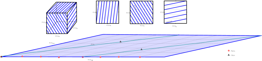
  Figure 1: The three-torus $U(1)_{\psi}\times U(1)_{\eta}\times U(1)_{\xi}$ broken to $U(1)_{\psi\xi}\times U(1)_{\eta\xi}$ for the $\{{\cal S},3,1\}$ model.

• For $p=2$, $N$ odd, ${\cal H}$ has only one connected component. In Figure 2 we show the graphs for the case $N=3$. One possible way to parameterize H is

  $${\cal H}=\frac{U(1)_{\psi\xi}\times U(1)_{\eta\xi}}{\mathbb{Z}_{2}}$$ (3.55)

  Note that $U(1)_{\psi\xi}$ contains $({\mathbbm{Z}}_{N+2})_{\psi}\times({\mathbbm{Z}}_{2})_{\xi}$ and $U(1)_{\eta\xi}$ contains $({\mathbbm{Z}}_{N+6})_{\eta}\times({\mathbbm{Z}}_{2})_{\xi}$ so $U(1)_{\psi\xi}\times U(1)_{\eta\xi}$ contains ${\mathbbm{Z}}_{2(N+2)}\times{\mathbbm{Z}}_{2(N+6)}$ which twice redundant with respect to $({\mathbbm{Z}}_{N+2})_{\psi}\times({\mathbbm{Z}}_{N+6})_{\eta}\times({\mathbbm{Z}}_{2})_{\xi}$. We can also see this in the following way. $U(1)_{\psi\xi}$ contains a non-trivial element of $U(1)_{\eta\xi}$. If we take the element of $U(1)_{\psi\xi}$ with $\beta=\pi$ we obtain

  $$\psi\to\psi\ ,\quad\eta\to\eta\ ,\quad\xi\to-\xi\$$ (3.56)

  which is exactly the element of $U(1)_{\eta\xi}$ with $\gamma=\pi$. This is the reason for the $\mathbb{Z}_{2}$ division in (3.55). The group $\widetilde{U}(1)$ that contains $\mathbb{Z}_{N}$ is the one generated by (3.54). If we define $\widehat{U}(1)$ generated by

  $${\bf t}_{\scriptscriptstyle\widehat{U}(1)}=-\frac{1}{2}{\bf t}_{\scriptscriptstyle U(1)_{\psi\xi}}+\frac{1}{2}{\bf t}_{\scriptscriptstyle U(1)_{\eta\xi}}\;,$$ (3.57)

  we can write

  $${\cal H}=U(1)_{\psi\xi}\times\widehat{U}(1)=U(1)_{\eta\xi}\times\widehat{U}(1)\;.$$ (3.58)

  

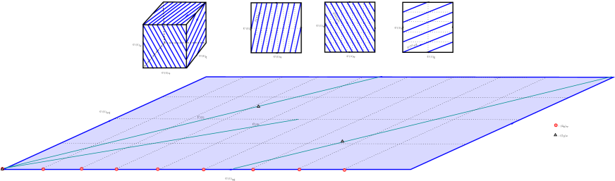
  Figure 2: The three-torus $U(1)_{\psi}\times U(1)_{\eta}\times U(1)_{\xi}$ broken to $\frac{U(1)_{\psi\xi}\times U(1)_{\eta\xi}}{\mathbb{Z}_{2}}$ for the $\{{\cal S},3,2\}$ model.

• For $p=2$, $N$ even, ${\cal H}$ has two components. In Figure 3, we illustrate the case $N=4$, $p=2$. One possible way to parameterize ${\cal H}$ is

  $${\cal H}=U(1)_{\psi\xi}\times U(1)_{\eta\xi}\times(\mathbb{Z}_{2})_{F}\;.$$ (3.59)

  We can define the group $\widetilde{U}(1)$ generated by (3.54) but this time it contains only $\mathbb{Z}_{\frac{N}{2}}$. In general it is not possible to write $\mathbb{Z}_{{N}}\subset U(1)^{\prime}\times(\mathbb{Z}_{2})_{F}$, both $U(1)$’s are necessary, although $N=4$, $p=2$ is an exception as we will see in the warmup example in Sec. 4.1.

  

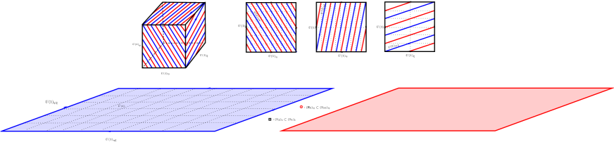
  Figure 3: The three-torus $U(1)_{\psi}\times U(1)_{\eta}\times U(1)_{\xi}$ broken to $U(1)_{\psi\xi}\times U(1)_{\eta\xi}\times(\mathbb{Z}_{2})_{F}$ for the $\{{\cal S},4,2\}$ model.

4 Mixed $({\mathbbm{Z}}_{2})_{F}-[{\mathbbm{Z}}_{N}]^{2}$ anomaly

The generalized (mixed) anomaly of the type $({\mathbbm{Z}}_{2})_{F}-[{\mathbbm{Z}}_{N}]^{2}$ was studied in detail in [2] for the $\{{\cal S},N,0\}$ (“$\psi\eta$”) model. We have briefly reviewed the method and results found there at the end of Introduction. This study is extended below to a wider class of models discussed in Sec. 2 and Sec. 3. The global structure of the anomaly-free symmetry group revealed in Sec. 3 teaches us that the most interesting class of models for the present purpose are $\{{\cal S},N,p\}$ and $\{{\cal A},N,p\}$ models with $N$ and $p$ both even, on which our analysis below will set focus.

4.1 A warmup example $\{{\cal S},4,2\}$

We first consider a simplest, nontrivial model $\{{\cal S},4,2\}$ and set up the calculation of the mixed anomalies, making a brief note on some general features of the gauging of the discrete 1-form ${\mathbbm{Z}}_{N}$ symmetry, on the idea of “$({\mathbbm{Z}}_{2})_{F}$ gauge field”, and paying special attention to the way the fermions transform nontrivially under the 1-form ${\mathbbm{Z}}_{N}$ gauge transformation. The same procedure can then be easily extended to more general cases discussed later.

Even though the fact that

$${\mathbbm{Z}}_{N}\subset U(1)_{\psi\xi}\times U(1)_{\eta\xi}\times({\mathbbm{Z}}_{2})_{F}\;$$ (4.1)

has been proven in general in Sec. 3.2, we need an explicit solution for this model, to fix the charges of the fermion fields under the 1-form ${\mathbbm{Z}}_{N}$ symmetry. From

$$U(1)_{\psi\xi}:\qquad\psi:\,e^{i\beta}\;;\quad\xi:\,e^{-i\tfrac{N+2}{2}\beta}=e^{-3i\beta}\;;$$

$$U(1)_{\eta\xi}:\qquad\eta:\,e^{i\gamma}\;;\quad\xi:\,e^{-i\tfrac{N+6}{2}\gamma}=e^{-5i\gamma}\;;$$

$${\mathbbm{Z}}_{N}:\qquad\psi:\,e^{4\pi i/N}=e^{\pi i}\;;\quad\eta:\,e^{-2\pi i/N}=e^{-i\pi/2}\;;\quad\xi:\,e^{2\pi i/N}=e^{i\pi/2}\;;$$

$${\mathbbm{Z}}_{2}:\qquad\psi:\,e^{\pm i\pi}\;;\quad\eta:\,e^{\pm i\pi}\;;\quad\xi:\,e^{\pm i\pi}\;,$$ (4.2)

we see that a simple solution in this case is to take $\beta=0$, and $\gamma=+\frac{\pi}{2}\;.$ It is easily seen that ${\mathbbm{Z}}_{N}$ is realized as a $U_{\eta\xi}(1)\times({\mathbbm{Z}}_{2})_{F}$ transformation with

$${\mathbbm{Z}}_{2}:\qquad\psi:\,e^{+i\pi}\;;\quad\eta:\,e^{-i\pi}\;;\quad\xi:\,e^{+3i\pi}\;.$$ (4.3)

We introduce accordingly,

• $A$: $U(1)_{\eta\xi}$ 1-form gauge field,

• $A_{2}$: $(\mathbb{Z}_{2})_{F}$ 1-form gauge field,

• ${\tilde{a}}$: $U(N)_{\rm c}$ 1-form gauge field,

• $B^{(2)}_{\mathrm{c}}$: $\mathbb{Z}_{N}$ 2-form gauge field.

The original $SU(N)$ gauge field $a$ is embedded in a $U(N)$ gauge field ${\tilde{a}}$ as

$$\widetilde{a}=a+{1\over N}B^{(1)}_{\mathrm{c}}\,,\qquad NB_{\mathrm{c}}^{(2)}=dB_{\mathrm{c}}^{(1)}\;.$$ (4.4)

As explained in [3], [4], one defines this way a globally well-defined $SU(N)/{\mathbbm{Z}}_{N}$ connection. The imposition of the local, 1-form gauge invariance (4.6) below, eliminates the apparent increase of the degrees of freedom (in going from $SU(N)$ to $U(N)$) on the one hand, and at the same time allows to “gauge away” the center ${\mathbbm{Z}}_{N}$ variation of Polyakov or Wilson loops

$$e^{i\oint a}\to e^{2\pi i/N}\,e^{i\oint a}\;,$$ (4.5)

on the other.

The 1-form gauge transformation acts on these fields as:

$$B^{(2)}_{\mathrm{c}} \to B^{(2)}_{\mathrm{c}}+{\mathrm{d}}\lambda_{\mathrm{c}}\;,\qquad\ \,B^{(1)}_{\mathrm{c}}\to B^{(1)}_{\mathrm{c}}+{N}\lambda_{\mathrm{c}}\;,$$

$${\tilde{a}} \to{\tilde{a}}+\lambda_{\mathrm{c}}\;,\qquad\qquad{F}({\tilde{a}})\to{F}({\tilde{a}})+d\lambda_{\mathrm{c}};,$$ (4.6)

$$A \to A-\lambda_{\mathrm{c}}\;,$$

$$A_{2} \to A_{2}+\frac{N}{2}\lambda_{\mathrm{c}}=A_{2}+2\lambda_{\mathrm{c}}\;.$$ (4.7)

As we are here dealing with a ${\mathbbm{Z}}_{N}$ which is a color-flavor locked symmetry the fermion fields also transform as well, appropriately. Their charges above follow from Eq. (4.2), Eq. (4.3).

It is perhaps not useless, before proceeding, to remind ourselves of the meaning of a “$({\mathbbm{Z}}_{2})_{F}$ gauge field”, $A_{2}$, which formally looks like an ordinary $U(1)$ gauge field. Restoring momentarily the suffices for the differential forms,

$$2A_{2}^{(1)}-B_{\mathrm{c}}^{(1)}=dA_{2}^{(0)}\;$$ (4.8)

can be regarded as an invariant form of the $({\mathbbm{Z}}_{2})_{F}$ gauge field, $2A_{2}^{(1)}=dA_{2}^{(0)}$, where $A_{2}^{(0)}$ is a $2\pi$ periodic scalar function (angle). It is an example of an “almost flat connection”: it satisfies $2\,\mathrm{d}A_{2}^{(1)}-{N}B_{\mathrm{c}}^{(2)}=0$ locally. However it cannot be set to zero everywhere, as a non vanishing flux through a closed two-dimensional surface may be present, allowing a nontrivial $({\mathbbm{Z}}_{2})_{F}$ holonomy $\oint A_{2}^{(1)}={2\pi m}/{2}\;,\,\,\,m\in{\mathbbm{Z}}$, along a noncontractible closed loop. A kind of partial gauge fixing would allow us to work with the gauge field $B_{\mathrm{c}}^{(1)}$ and gauge function $\lambda_{\mathrm{c}}$, satisfying always

$$\oint B_{\mathrm{c}}^{(1)}=2\pi n\;,\qquad\oint\lambda_{\mathrm{c}}=\frac{2\pi\ell}{N}\;,\qquad\quad(n\in{\mathbbm{Z}},\quad\ell\in{\mathbbm{Z}})\;.$$ (4.9)

See [2] for more discussions.

The fermion kinetic terms are:

$$\overline{\psi}\gamma^{\mu}\big{(}\partial+\mathcal{R}_{\mathrm{S}}(\widetilde{a})-A_{2}\big{)}_{\mu}P_{\mathrm{L}}\psi+$$

$$\overline{\eta}\gamma^{\mu}\big{(}\partial+\mathcal{R}_{\mathrm{F}^{*}}(\widetilde{a})+A+A_{2}\big{)}_{\mu}P_{\mathrm{L}}\eta+$$

$$\overline{\xi}\gamma^{\mu}\big{(}\partial+\mathcal{R}_{\mathrm{F}}(\widetilde{a})-5A-3A_{2}\big{)}_{\mu}P_{\mathrm{L}}\xi\;,$$ (4.10)

each of which is indeed invariant under (4.6) and (4.7). Note that the choice of the ${\mathbbm{Z}}_{2}$ charges, ($1,-1,+3$) for ($\psi,\eta,\xi$) fields (see Eq. (4.3)) is dictated by the requirement that the redundancy (4.1) involving the discrete symmetries ${\mathbbm{Z}}_{2}$ and ${\mathbbm{Z}}_{N}$ be formally expressed as an invariance under (4.6) with a continuous gauge function $\lambda_{c}=\lambda_{c}^{\mu}(x)\,dx_{\mu}$. The 1-form gauge invariant field tensors are, for the UV fermions $\psi$, $\eta$, $\xi$,

$$\mathcal{R}_{\mathrm{S}}F(\tilde{a})-{\mathrm{d}}A_{2}\;,$$

$$\mathcal{R}_{\mathrm{F}}^{*}F(\tilde{a})+{\mathrm{d}}A+{\mathrm{d}}A_{2}\;,$$

$$\mathcal{R}_{\mathrm{F}}F(\tilde{a})-5\,{\mathrm{d}}A-3\,{\mathrm{d}}A_{2}\;.$$ (4.11)

By rearranging things so that each term in the bracket is manifestly invariant under (4.6) and (4.7), this can be rewritten as

$$\mathcal{R}_{\mathrm{S}}\big{(}F(\tilde{a})-B^{(2)}_{\mathrm{c}}\big{)}-\left({\mathrm{d}}A_{2}-2B^{(2)}_{\mathrm{c}}\right)\;,$$

$$\mathcal{R}_{\mathrm{F}}^{*}\big{(}F(\tilde{a})-B^{(2)}_{\mathrm{c}}\big{)}+({\mathrm{d}}A+B^{(2)}_{\mathrm{c}})+\left({\mathrm{d}}A_{2}-2B^{(2)}_{\mathrm{c}}\right)\;,$$

$$\mathcal{R}_{\mathrm{F}}\big{(}F(\tilde{a})-B^{(2)}_{\mathrm{c}}\big{)}-5\,({\mathrm{d}}A+B^{(2)}_{\mathrm{c}})-3\,\left({\mathrm{d}}A_{2}-2B^{(2)}_{\mathrm{c}}\right)\;.$$ (4.12)

In the confining vacuum with the full global symmetry, discussed in Sec. 2.3, the infrared degrees of freedom would be the (massless, by assumption) composite fermions ${\cal B}_{1}$, ${\cal B}_{2}$, ${\cal B}_{3}$, (2.19). Their kinetic terms are given by

$$\overline{{\cal B}_{1}}\gamma^{\mu}\big{(}\partial+2A+A_{2}\big{)}_{\mu}P_{\mathrm{L}}{\cal B}_{1}+$$

$$\overline{{\cal B}_{2}}\gamma^{\mu}\big{(}\partial-6A-3A_{2}\big{)}_{\mu}P_{\mathrm{L}}{\cal B}_{2}+$$

$$\overline{{\cal B}_{3}}\gamma^{\mu}\big{(}\partial+10A+5A_{2}\big{)}_{\mu}P_{\mathrm{L}}{\cal B}_{3}\;.$$ (4.13)

The corresponding invariant tensors are

$$2\,({\mathrm{d}}A+B^{(2)}_{\mathrm{c}})+\left[{\mathrm{d}}A_{2}-2B^{(2)}_{\mathrm{c}}\right]\;,$$

$$-6\,({\mathrm{d}}A+B^{(2)}_{\mathrm{c}})-3\left[{\mathrm{d}}A_{2}-2B^{(2)}_{\mathrm{c}}\right]\;,$$

$$10\,({\mathrm{d}}A+B^{(2)}_{\mathrm{c}})+5\left[{\mathrm{d}}A_{2}-2B^{(2)}_{\mathrm{c}}\right]\;,$$ (4.14)

respectively. Though this formula appears to depend on $B^{(2)}_{\mathrm{c}}$ due to the way things have been arranged to make each term manifestly invariant, $B^{(2)}_{\mathrm{c}}$ actually drops out completely, reflecting the fact that ${\cal B}_{1}$, ${\cal B}_{2}$, ${\cal B}_{3}$ are all color $SU(N)$ singlets: there are no gauge kinetic terms in their action. As a result, there would be no mixed anomalies in the IR due to the gauging of ${\mathbbm{Z}}_{N}$ 1-form symmetry.

Note that the same cannot be said of the formula Eq. (4.12) in the UV theory. Because, for instance,

$$\mathrm{tr}\,F(\tilde{a})=N\,B^{(2)}_{\mathrm{c}}\;,$$ (4.15)

for the fundamental representation, the $B^{(2)}_{\mathrm{c}}$ dependence of the expressions in Eq. (4.12) is not exhausted by the explicit $B^{(2)}_{\mathrm{c}}$ factors. Even though we shall use the formula Eq. (4.12) for the calculation of the mixed anomalies below, for manifest 1-form gauge invariance of our calculation step by step, the same final result can be obtained (as it should) by working with a not-term-by-term-manifestly-invariant expression Eq. (LABEL:tensors00). This is shown in Appendix A. As a bonus, the discussion there explains some interesting aspect of our results below.

The rest of the calculations follows that done in [2]. From Eq. (4.1) one finds the $6D$ anomaly functional in the UV theory ,

$${1\over 24\pi^{2}}\,{\mathrm{tr}}_{\mathcal{R}_{\mathrm{S}}}\left[\left\{\big{(}{F}({\tilde{a}})-B^{(2)}_{\mathrm{c}}\big{)}-\left({\mathrm{d}}A_{2}-2B^{(2)}_{\mathrm{c}}\right)\right\}^{3}\right]+$$

$${1\over 24\pi^{2}}\,{\mathrm{tr}}_{\mathcal{R}_{\mathrm{F}}^{*}}\left[\left\{\big{(}{F}({\tilde{a}})-B^{(2)}_{\mathrm{c}}\big{)}+({\mathrm{d}}A+B^{(2)}_{\mathrm{c}})+\left({\mathrm{d}}A_{2}-2B^{(2)}_{\mathrm{c}}\right)\right\}^{3}\right]+$$

$${1\over 24\pi^{2}}\,{\mathrm{tr}}_{\mathcal{R}_{\mathrm{F}}}\left[\left\{\big{(}{F}({\tilde{a}})-B^{(2)}_{\mathrm{c}}\big{)}-5({\mathrm{d}}A+B^{(2)}_{\mathrm{c}})-3\left({\mathrm{d}}A_{2}-2B^{(2)}_{\mathrm{c}}\right)\right\}^{3}\right]\;.$$ (4.16)

Keeping only the relevant terms, the first line ($\psi$) gives

$${1\over 24\pi^{2}}\left[-3(N+2){\mathrm{tr}}\big{(}F(\tilde{a})-B^{(2)}_{\mathrm{c}}\big{)}^{2}\Big{(}{\mathrm{d}}A_{2}-2B^{(2)}_{\mathrm{c}}\Big{)}-\frac{N(N+1)}{2}\Big{(}{\mathrm{d}}A_{2}-2B^{(2)}_{\mathrm{c}}\Big{)}^{3}\right]\;,$$ (4.17)

the second line ($\eta$) gives

$${1\over 24\pi^{2}}\left[3(N+6){\mathrm{tr}}\big{(}F(\tilde{a})-B^{(2)}_{\mathrm{c}}\big{)}^{2}\Big{(}{\mathrm{d}}A_{2}-\frac{N}{2}B^{(2)}_{\mathrm{c}}\Big{)}+N(N+6)\Big{(}{\mathrm{d}}A_{2}-B^{(2)}_{\mathrm{c}}+\dots\Big{)}^{3}\right]\;,$$ (4.18)

the third line ($\xi$) gives:

$${1\over 24\pi^{2}}\left[-3\cdot 2\cdot 3\,{\mathrm{tr}}\big{(}F(\tilde{a})-B^{(2)}_{\mathrm{c}}\big{)}^{2}\Big{(}{\mathrm{d}}A_{2}-\frac{N}{2}B^{(2)}_{\mathrm{c}}\Big{)}+2N\Big{(}-3\,{\mathrm{d}}A_{2}+B^{(2)}_{\mathrm{c}}+\ldots\Big{)}^{3}\right]\;.$$ (4.19)

Collecting the relevant terms, one finds that the coefficient of

$${1\over 8\pi^{2}}(B^{(2)}_{\mathrm{c}})^{2}\,{\mathrm{d}}A_{2}$$ (4.20)

is equal to

$$N(N+2)-\frac{N(N+1)}{2}4+(N+6)(-N)+N(N+6)+2N3+2N(-3)$$

$$=-N^{2}=-16\;.$$ (4.21)

Following the usual procedure (e.g., Eq. (1.15), Eq. (1.16)) we find the mixed $({\mathbbm{Z}}_{2})_{F}-[{\mathbbm{Z}}_{N}]^{2}$ anomaly in $4D$:

$$-N^{2}\,{1\over 8\pi^{2}}\int_{\Sigma^{4}}(B^{(2)}_{\mathrm{c}})^{2}\,\frac{1}{2}\delta A_{2}^{(0)}=-N^{2}\times\frac{\mathbbm{Z}}{N^{2}}\,({\pm\pi})=\pm\pi\times{\mathbbm{Z}}\;.$$ (4.22)

Namely, the partition function suffers from a sign change under the fermion parity transformation. On the other hand, one would find no $({\mathbbm{Z}}_{2})_{F}$ anomaly in the IR, if one would assume the chirally symmetric vacuum with the massless baryons ${\cal B}_{1}$, ${\cal B}_{2}$, ${\cal B}_{3}$ of Sec. 2.3. The contradiction can be avoided by assuming that the system actually is in a dynamical Higgs phase such as the one discussed in Sec. 2.4.

4.2 General $\{{\cal S},N,p\}$ models with generic $N$ and $p$ even

Let us now discuss $\{{\cal S},N,p\}$ systems with general $N$, $p$, both even. As in the warmup example, we verify anew

$${\mathbbm{Z}}_{N}\subset U(1)_{\psi\eta}\times U(1)_{\psi\xi}\times{\mathbbm{Z}}_{2}\;$$ (4.23)

for $N$, $p$ both even, by solving the equations :

$$\frac{N+4+p}{2}{\alpha}+\frac{p}{2}\,{\beta} = \frac{4\pi}{N}\pm\pi\;,$$

$$-\frac{N+2}{2}{\alpha} = -\frac{2\pi}{N}\pm\pi\;,$$

$$-\frac{N+2}{2}{\beta} = \frac{2\pi}{N}\pm\pi\;,$$ (4.24)

concretely. Indeed, it is sufficient to find one good solution. A possible solution is

$${\alpha}=\frac{4\pi}{N(N+2)}+\frac{2\pi}{N+2}\;,\qquad{\beta}=-\frac{4\pi}{N(N+2)}-\frac{2\pi}{N+2}\;,$$ (4.25)

which is a solution with the $({\mathbbm{Z}}_{2})_{F}$ signs $+,-,+$ for the $\psi,\eta,\xi$ fields in Eq. (4.24), respectively. The above solution Eq. (4.25) can be simply rewritten as

$${\alpha}=\frac{2\pi}{N}\;,\quad{\beta}=-\frac{2\pi}{N}\;.$$ (4.26)

As in any anomaly calculation we couple the system to the appropriate background gauge fields,

• $A_{\psi\eta}$: $U(1)_{\psi\eta}$ 1-form gauge field,

• $A_{\psi\xi}$: $U(1)_{\psi\xi}$ 1-form gauge field,

• $A_{2}$: $(\mathbb{Z}_{2})_{F}$ 1-form gauge field,

• ${\tilde{a}}$: $U(N)_{\rm c}$ 1-form gauge field,

• $B^{(2)}_{\mathrm{c}}$: $\mathbb{Z}_{N}$ 2-form gauge field.

Under the 1-form gauge transformation the fields transform as

$$B^{(2)}_{\mathrm{c}} \to B^{(2)}_{\mathrm{c}}+{\mathrm{d}}\lambda_{\mathrm{c}}\;,\qquad\ \,B^{(1)}_{\mathrm{c}}\to B^{(1)}_{\mathrm{c}}+{N}\lambda_{\mathrm{c}}\;,$$

$${\tilde{a}} \to{\tilde{a}}+\lambda_{c}\;,\qquad\qquad\ {\tilde{F}}({\tilde{a}})\to{\tilde{F}}({\tilde{a}})+d\lambda_{c}\;,$$

$$A_{\psi\eta} \to A_{\psi\eta}-\lambda_{c}\;,$$

$$A_{\psi\xi} \to A_{\psi\xi}+\lambda_{c}\;,$$

$$A_{2} \to A_{2}+\frac{N}{2}\lambda_{c}\;,$$ (4.27)

where the charges follow from (4.24) and (4.26). The fermion kinetic terms are:

$$\overline{\psi}\gamma^{\mu}\Big{(}\partial+\mathcal{R}_{\mathrm{S}}(\widetilde{a})+\frac{N+4+p}{2}A_{\psi\eta}+\frac{p}{2}A_{\psi\xi}+A_{2}\Big{)}_{\mu}P_{\mathrm{L}}\psi+$$

$$\overline{\eta}\gamma^{\mu}\Big{(}\partial+\mathcal{R}_{\mathrm{F}^{*}}(\widetilde{a})-\frac{N+2}{2}A_{\psi\eta}-A_{2}\Big{)}_{\mu}P_{\mathrm{L}}\eta+$$

$$\overline{\xi}\gamma^{\mu}\Big{(}\partial+\mathcal{R}_{\mathrm{F}}(\widetilde{a})-\frac{N+2}{2}A_{\psi\xi}+A_{2}\Big{)}_{\mu}P_{\mathrm{L}}\xi\;.$$ (4.28)

It can be checked readily that each line is invariant under Eq. (4.2). In particular, the $({\mathbbm{Z}}_{2})_{F}$ charges are fixed by this requirement.

The 1-form gauge invariant field tensors are, for the UV fermions $\psi$, $\eta$, $\xi$,

$$\!\!\!\!{\cal T}_{1}=\mathcal{R}_{\mathrm{S}}\big{(}F(\tilde{a})-B^{(2)}_{\mathrm{c}}\big{)}+\frac{N+4+p}{2}({\mathrm{d}}A_{\psi\eta}+B^{(2)}_{\mathrm{c}})+\frac{p}{2}({\mathrm{d}}A_{\psi\xi}-B^{(2)}_{\mathrm{c}})+\Big{(}{\mathrm{d}}A_{2}-\frac{N}{2}B^{(2)}_{\mathrm{c}}\Big{)},$$

$$\!\!\!\!{\cal T}_{2}=\mathcal{R}_{\mathrm{F}}^{*}\big{(}F(\tilde{a})-B^{(2)}_{\mathrm{c}}\big{)}-\frac{N+2}{2}({\mathrm{d}}A_{\psi\eta}+B^{(2)}_{\mathrm{c}})-\Big{(}{\mathrm{d}}A_{2}-\frac{N}{2}B^{(2)}_{\mathrm{c}}\Big{)}\;,$$

$$\!\!\!\!{\cal T}_{3}=\mathcal{R}_{\mathrm{F}}\big{(}F(\tilde{a})-B^{(2)}_{\mathrm{c}}\big{)}-\frac{N+2}{2}({\mathrm{d}}A_{\psi\xi}-B^{(2)}_{\mathrm{c}})+\Big{(}{\mathrm{d}}A_{2}-\frac{N}{2}B^{(2)}_{\mathrm{c}}\Big{)}\;,$$ (4.29)

where appropriate factors of $B^{(2)}_{\mathrm{c}}$ are added and subtracted so that each term in the bracket is invariant under the 1-form gauge transformations (4.2). Of course, the final result does not depend on such a rewriting: see Appendix A.

The $6D$ anomaly functional is

$${1\over 24\pi^{2}}\,\int\,{\mathrm{tr}}_{\mathcal{R}_{\mathrm{S}}}({\cal T}_{1})^{3}+{1\over 24\pi^{2}}\,\int\,{\mathrm{tr}}_{\mathcal{R}_{\mathrm{F}}^{*}}({\cal T}_{2})^{3}+{1\over 24\pi^{2}}\,\int\,{\mathrm{tr}}_{\mathcal{R}_{\mathrm{F}}}({\cal T}_{3})^{3}\;.$$ (4.30)

Let us now extract the terms relevant to the $({\mathbbm{Z}}_{2})_{F}-[{\mathbbm{Z}}_{N}]^{2}$ anomaly. From the $\psi$ contribution one has

$${1\over 24\pi^{2}}\left[3(N+2){\mathrm{tr}}\big{(}F(\tilde{a})-B^{(2)}_{\mathrm{c}}\big{)}^{2}\Big{(}{\mathrm{d}}A_{2}-\frac{N}{2}B^{(2)}_{\mathrm{c}}\Big{)}+\frac{N(N+1)}{2}\Big{(}{\mathrm{d}}A_{2}+2B^{(2)}_{\mathrm{c}}+\ldots\Big{)}^{3}\right]\;,$$ (4.31)

$\eta$ gives

$${1\over 24\pi^{2}}\left[3(N+4+p){\mathrm{tr}}\big{(}F(\tilde{a})-B^{(2)}_{\mathrm{c}}\big{)}^{2}\Big{(}{\mathrm{d}}A_{2}-\frac{N}{2}B^{(2)}_{\mathrm{c}}\Big{)}-N(N+4+p)\Big{(}{\mathrm{d}}A_{2}+B^{(2)}_{\mathrm{c}}+\ldots\Big{)}^{3}\right]$$ (4.32)

and the third line ($\xi$) gives:

$${1\over 24\pi^{2}}\left[3p\,{\mathrm{tr}}\big{(}F(\tilde{a})-B^{(2)}_{\mathrm{c}}\big{)}^{2}\Big{(}{\mathrm{d}}A_{2}-\frac{N}{2}B^{(2)}_{\mathrm{c}}\Big{)}+pN\Big{(}\,{\mathrm{d}}A_{2}+B^{(2)}_{\mathrm{c}}+\ldots\Big{)}^{3}\right]\;.$$ (4.33)

Collecting terms, one finds that the coefficient of

$${1\over 8\pi^{2}}(B^{(2)}_{\mathrm{c}})^{2}\,{\mathrm{d}}A_{2}$$ (4.34)

is equal to

$$-N(N+2)+\frac{N(N+1)}{2}\cdot 4-N(N+4+p)+N(N+4+p)-Np+pN$$

$$=N^{2}\;.$$ (4.35)

A somewhat curious feature of this result (and of Eq. (4.21)) is that only fermions in a higher representation contribute to the anomaly. The reason for this will become clear in an alternative derivation discussed in Appendix A.

Following the usual procedure one calculates the $4D$ mixed $({\mathbbm{Z}}_{2})_{F}-[{\mathbbm{Z}}_{N}]^{2}$ anomaly. One finds an extra phase in the partition function associated with the fermion parity transformation in the presence of the ${\mathbbm{Z}}_{N}$ gauge fields,

$$N^{2}\,{1\over 8\pi^{2}}\int_{\Sigma^{4}}(B^{(2)}_{\mathrm{c}})^{2}\,\frac{1}{2}\delta A_{2}^{(0)}=N^{2}\times\frac{\mathbbm{Z}}{N^{2}}\,({\pm\pi})=\pm\pi\times{\mathbbm{Z}}\;:$$ (4.36)

there is a $({\mathbbm{Z}}_{2})_{F}-[{\mathbbm{Z}}_{N}]^{2}$ mixed anomaly in the theory.

On the other hand, one finds no $({\mathbbm{Z}}_{2})_{F}$ anomaly in the IR, if one assumes the symmetric vacuum of Sec. 2.3. This can be seen, as in the warmup example of the previous section, by simply noting that all infrared degrees of freedom are color-singlet. We conclude that the chirally symmetric vacuum described by the baryons ${\cal B}_{1}$, ${\cal B}_{2}$, ${\cal B}_{3}$ cannot be realized dynamically.

We note again that such an inconsistency is avoided, assuming that the system is in the dynamical Higgs phase: the color-flavor locked 1-form symmetry is spontaneously broken.

4.3 $\{{\cal A},N,p\}$ models with $N$ and $p$ even

The simplest of this class of models, $\{{\cal A},N,0\}$, with matter fermions

$$\yng(1,1)\oplus(N-4)\,{\bar{{\yng(1)}}}\;,$$ (4.37)

(“$\chi\eta$ model”), has been studied, and the result of the analysis (unpublished) turns out to be similar to that in the $\psi\eta$ model of [2], reviewed in Introduction. For even $N$ the (nonanomalous) symmetry of the system contains a nonanomalous $(\mathbb{Z}_{2})_{F}$ factor orthogonal to other continuous symmetry group. It gets anomalous under the 1-form gauging of a ${\mathbbm{Z}}_{N}$ center symmetry. This anomaly cannot be reproduced in the infrared, if the vacuum is assumed to be confining, and to keep the full global symmetries. Such a vacuum cannot be realized dynamically.

Below we study a more general class of $\{{\cal A},N,p\}$ models, with $p$ additional pairs of fermions in $\yng(1)\oplus{\bar{\yng(1)}}$. We check first

$${\mathbbm{Z}}_{N}\subset U(1)_{\chi\eta}\times U(1)_{\chi\xi}\times{\mathbbm{Z}}_{2}\;.$$ (4.38)

Call $\alpha$ and $\beta$ the angles associated with $U(1)_{\chi\eta}$ and $U(1)_{\chi\xi}\,$,

$$U(1)_{\chi\eta}:\qquad\chi\to\mathrm{e}^{\mathrm{i}\tfrac{N-4+p}{2}\alpha}\chi\;,\quad\eta\to\mathrm{e}^{-\mathrm{i}\tfrac{N-2}{2}\alpha}\eta\;,$$

$$U(1)_{\chi\xi}:\qquad\chi\to\mathrm{e}^{\mathrm{i}\tfrac{p}{2}\beta}\chi\;,\quad\xi\to\mathrm{e}^{-\mathrm{i}\tfrac{N-2}{2}\beta}\xi\;.$$ (4.39)

The condition (4.38) means that

$$\frac{N-4+p}{2}{\alpha}+\frac{p}{2}\,{\beta} = \frac{4\pi}{N}\pm\pi\;,$$

$$-\frac{N-2}{2}{\alpha} = -\frac{2\pi}{N}\pm\pi\;,$$

$$-\frac{N-2}{2}{\beta} = \frac{2\pi}{N}\pm\pi\;.$$ (4.40)

It turns out that any two of these imply the third: there is an arbitrariness to choose from multiple of solutions. A possible solution is

$${\alpha}=\frac{4\pi}{N(N-2)}-\frac{2\pi}{N-2}\;,\qquad{\beta}=-\frac{4\pi}{N(N-2)}+\frac{2\pi}{N-2}\;,$$ (4.41)

which is a solution with the $({\mathbbm{Z}}_{2})_{F}$ signs in Eq. (4.40), $-\pi,+\pi,-\pi$ for the $\chi,\eta,\xi$ fields, respectively. Actually the solution Eq. (4.41) is, simply,

$${\alpha}=-\frac{2\pi}{N}\;,\qquad{\beta}=\frac{2\pi}{N}\;.$$ (4.42)

The color-flavor locked ${\mathbbm{Z}}_{N}$ transformation, (4.40) and (4.42), together with the normalization of the 1-form gauge field $\lambda_{c}$, fix the charges of the fermion fields in Eq. (4.44) below.

We introduce the background gauge fields

• $A_{\chi\eta}$: $U(1)_{\chi\eta}$ 1-form gauge field,

• $A_{\chi\xi}$: $U(1)_{\chi\xi}$ 1-form gauge field,

• $A_{2}$: $(\mathbb{Z}_{2})_{F}$ 1-form gauge field field,

• ${\tilde{a}}$: $U(N)_{\rm c}$ 1-form gauge field,

• $B^{(2)}_{\mathrm{c}}$: $\mathbb{Z}_{N}$ 2-form gauge field.

Under the 1-form gauge transformation

$$B^{(2)}_{\mathrm{c}} \to B^{(2)}_{\mathrm{c}}+{\mathrm{d}}\lambda_{\mathrm{c}}\;,\qquad\ \,B^{(1)}_{\mathrm{c}}\to B^{(1)}_{\mathrm{c}}+{N}\lambda_{\mathrm{c}}\;,$$

$${\tilde{a}} \to{\tilde{a}}+\lambda_{c}\;,\qquad\qquad\ {\tilde{F}}({\tilde{a}})\to{\tilde{F}}({\tilde{a}})+d\lambda_{c}\;,$$

$$A_{\chi\eta} \to A_{\chi\eta}+\lambda_{c}\;,\qquad$$

$$A_{\chi\xi} \to A_{\chi\xi}-\lambda_{c}\;,\qquad$$

$$A_{2} \to A_{2}+\frac{N}{2}\lambda_{c}\;.$$ (4.43)

The fermion kinetic terms are: (the charges follow from (4.42))

$$\overline{\chi}\gamma^{\mu}\Big{(}\partial+\mathcal{R}_{\mathrm{A}}(\widetilde{a})+\frac{N-4+p}{2}A_{\chi\eta}+\frac{p}{2}A_{\chi\xi}-A_{2}\Big{)}_{\mu}P_{\mathrm{L}}\chi+$$

$$\overline{\eta}\gamma^{\mu}\Big{(}\partial+\mathcal{R}_{\mathrm{F}^{*}}(\widetilde{a})-\frac{N-2}{2}A_{\chi\eta}+A_{2}\Big{)}_{\mu}P_{\mathrm{L}}\eta+$$

$$\overline{\xi}\gamma^{\mu}\Big{(}\partial+\mathcal{R}_{\mathrm{F}}(\widetilde{a})-\frac{N-2}{2}A_{\chi\xi}-A_{2}\Big{)}_{\mu}P_{\mathrm{L}}\xi\;.$$ (4.44)

It is seen that each line is invariant under (4.3). In particular, the $({\mathbbm{Z}}_{2})_{F}$ charges are fixed by this requirement.

The 1-form gauge invariant field tensors are, for the UV fermions $\chi$, $\eta$, $\xi$,

$$\!\!\!\!{\cal T}_{1}=\mathcal{R}_{\mathrm{A}}\big{(}F(\tilde{a})-B^{(2)}_{\mathrm{c}}\big{)}+\frac{N-4+p}{2}({\mathrm{d}}A_{\chi\eta}-B^{(2)}_{\mathrm{c}})+\frac{p}{2}({\mathrm{d}}A_{\chi\xi}+B^{(2)}_{\mathrm{c}})-\Big{(}{\mathrm{d}}A_{2}-\frac{N}{2}B^{(2)}_{\mathrm{c}}\Big{)},$$

$$\!\!\!\!{\cal T}_{2}=\mathcal{R}_{\mathrm{F}^{*}}\big{(}F(\tilde{a})-B^{(2)}_{\mathrm{c}}\big{)}-\frac{N-2}{2}({\mathrm{d}}A_{\chi\eta}-B^{(2)}_{\mathrm{c}})+\Big{(}{\mathrm{d}}A_{2}-\frac{N}{2}B^{(2)}_{\mathrm{c}}\Big{)}\;,$$

$$\!\!\!\!{\cal T}_{3}=\mathcal{R}_{\mathrm{F}}\big{(}F(\tilde{a})-B^{(2)}_{\mathrm{c}}\big{)}-\frac{N-2}{2}({\mathrm{d}}A_{\chi\xi}+B^{(2)}_{\mathrm{c}})-\Big{(}{\mathrm{d}}A_{2}-\frac{N}{2}B^{(2)}_{\mathrm{c}}\Big{)}\;.$$ (4.45)

The $6D$ anomaly functional is

$${1\over 24\pi^{2}}\,\int\,{\mathrm{tr}}_{\mathcal{R}_{\mathrm{A}}}({\cal T}_{1})^{3}+{1\over 24\pi^{2}}\,\int\,{\mathrm{tr}}_{\mathcal{R}_{\mathrm{F}^{*}}}({\cal T}_{2})^{3}+{1\over 24\pi^{2}}\,\int\,{\mathrm{tr}}_{\mathcal{R}_{\mathrm{F}}}({\cal T}_{3})^{3}\;.$$ (4.46)

Let us now extract the terms relevant to the $({\mathbbm{Z}}_{2})_{F}-[{\mathbbm{Z}}_{N}]^{2}$ anomaly. From the $\chi$ contribution one has

$${1\over 24\pi^{2}}\left[-3(N-2){\mathrm{tr}}\big{(}F(\tilde{a})-B^{(2)}_{\mathrm{c}}\big{)}^{2}\Big{(}{\mathrm{d}}A_{2}-\frac{N}{2}B^{(2)}_{\mathrm{c}}\Big{)}-\frac{N(N-1)}{2}\Big{(}{\mathrm{d}}A_{2}-2B^{(2)}_{\mathrm{c}}+\ldots\Big{)}^{3}\right]\;,$$ (4.47)

$\eta$ gives

$${1\over 24\pi^{2}}\left[3(N-4+p){\mathrm{tr}}\big{(}F(\tilde{a})-B^{(2)}_{\mathrm{c}}\big{)}^{2}\Big{(}{\mathrm{d}}A_{2}-\frac{N}{2}B^{(2)}_{\mathrm{c}}\Big{)}+N(N-4+p)\Big{(}{\mathrm{d}}A_{2}-B^{(2)}_{\mathrm{c}}+\ldots\Big{)}^{3}\right]$$ (4.48)

and the third line ($\xi$) gives:

$${1\over 24\pi^{2}}\left[-3p\,{\mathrm{tr}}\big{(}F(\tilde{a})-B^{(2)}_{\mathrm{c}}\big{)}^{2}\Big{(}{\mathrm{d}}A_{2}-\frac{N}{2}B^{(2)}_{\mathrm{c}}\Big{)}-pN\Big{(}\,{\mathrm{d}}A_{2}-B^{(2)}_{\mathrm{c}}+\ldots\Big{)}^{3}\right]\;.$$ (4.49)

Collecting terms, one finds that the coefficient of

$${1\over 8\pi^{2}}(B^{(2)}_{\mathrm{c}})^{2}\,{\mathrm{d}}A_{2}$$ (4.50)

is equal to

$$N(N-2)-\frac{N(N-1)}{2}\cdot 4+(N-4+p)(-N)+N(N-4+p)+Np-pN$$

$$=-N^{2}\;.$$ (4.51)

Following the usual procedure one calculates the $4D$ mixed $({\mathbbm{Z}}_{2})_{F}-[{\mathbbm{Z}}_{N}]^{2}$ anomaly,

$$-N^{2}\,{1\over 8\pi^{2}}\int_{\Sigma^{4}}(B^{(2)}_{\mathrm{c}})^{2}\,\frac{1}{2}\delta A_{2}^{(0)}=N^{2}\times\frac{\mathbbm{Z}}{N^{2}}\,({\pm\pi})=\pm\pi\times{\mathbbm{Z}}\;.$$ (4.52)

That is, the partition function changes sign under the fermion parity, $\chi,\eta,\xi\to-\chi,-\eta,-\xi$. In other words, we found a $({\mathbbm{Z}}_{2})_{F}-[{\mathbbm{Z}}_{N}]^{2}$ mixed anomaly in the UV theory.

On the other hand, one finds no $({\mathbbm{Z}}_{2})_{F}$ anomaly in the IR, assuming the chirally symmetric vacuum with the massless baryons ${\cal B}_{1}$, ${\cal B}_{2}$, ${\cal B}_{3}$. This then cannot be the correct phase of the system.

5 Summary

In this work we have extended the study of mixed anomalies affecting a chiral discrete $({\mathbbm{Z}}_{2})_{F}$ symmetry, found [2] in a simple chiral gauge theory ($\psi\eta$ model), to a wider class of models, the general Bars-Yankielowicz and the generalized Georgi-Glashow models.

Writing the effects of instantons on the three $U(1)$’s associated with the three fermions as

$$U(1)_{\psi}\times U(1)_{\eta}\times U(1)_{\xi}\xrightarrow{\rm anomaly}{\cal H}\;,$$ (5.1)

the global symmetry of these models $G_{\mathrm{f}}$ can be written, for $\{{\cal S},N,p\}$ models, for instance, as

$$G_{\mathrm{f}}\xrightarrow{\rm anomaly}\frac{SU(N+4+p)\times SU(p)\times{\cal H}}{\mathbb{Z}_{N}\times\mathbb{Z}_{N+4+p}\times\mathbb{Z}_{p}}\;$$ (5.2)

and similarly for $\{{\cal A},N,p\}$ models, with a replacement, $N+4+p\to N-4+p$. The division by various centers has been explained in Sec. 3.

In both classes of the models, if one of $N$ and $p$ (or both) is odd, ${\cal H}$, hence $G_{f}$, has a connected structure. It can be taken as

$${\cal H}=U(1)_{1}\times U(1)_{2}\;,$$ (5.3)

where $U(1)_{1,2}$ are arbitrary two of the nonanomalous combinations, $U(1)_{\psi\eta}$, $U(1)_{\psi\xi}$, and $U(1)_{\xi\eta}$. It follows that, once the conventional anomaly matching equations are all satisfied with respect to $G_{F}$, considering the mixed anomalies involving the 1-form discrete center symmetry $\mathbb{Z}_{N}$ does not provide us with any new information about the candidate phase of the system. The UV-IR matching involving any new, mixed anomalies is a simple consequence of (i.e., included in) the conventional anomaly matching equations. This is similar to what was found in [2] for odd $N$ $\psi\eta$ models.

For this reason, the main part of our analysis here has been focused on the models with $N$ and $p$, both even. In all cases of this type, the global symmetry $G_{f}$ has two, disconnected components, as

$${\cal H}=U(1)_{1}\times U(1)_{2}\times({\mathbbm{Z}}_{2})_{F}\;.$$ (5.4)

$({\mathbbm{Z}}_{2})_{F}$ is nonanomalous, as all other factors in $G_{F}$, but the fact that it is nonanomalous hinges upon the integer instanton numbers

$$\frac{1}{8\pi^{2}}\,\left(\int_{\Sigma_{4}}\mathrm{tr}\,F^{2}\right)\in{\mathbbm{Z}}$$ (5.5)

and is not a simple result of an algebraic cancellation of the contributions from different fermions, as is the case for the continuous, nonanomalous symmetries $U(1)_{\psi\xi}\times U(1)_{\eta\xi}$. This can be checked by inspecting Eqs. (4.13),  (4.28) and (4.44). For instance, in the warmup example of the $\{{\cal S},4,2\}$ model, the effect of the chiral transformations,

$$\psi\to e^{-i\pi}\psi\;,\quad\eta\to e^{i\pi}\eta\;,\quad\xi\to e^{-3i\pi}\xi\;,$$ (5.6)

(see Eq. (4.13)) is the extra phase in the partition function

$$\{-(N+2)+(N+6)-3\cdot 2\}\,\frac{1}{8\pi^{2}}\,\left(\int_{\Sigma_{4}}\mathrm{tr}\,F^{2}\right)\cdot\pi=-2\pi\,{\mathbbm{Z}}\;:$$ (5.7)

which is indeed irrelevant, but only because the instanton numbers are quantized to integers. The nonanomalous $({\mathbbm{Z}}_{2})_{F}$ symmetry has thus a different status as compared to other, continuous nonanomalous symmetries such as $U(1)_{\chi\eta},\,U(1)_{\chi\xi}\,$ and $U(1)_{\eta\xi}$.

But this means that, once all fields are coupled to the 1-form center ${\mathbbm{Z}}_{N}$ gauge fields $\big{(}B_{\mathrm{c}}^{(2)},B_{\mathrm{c}}^{(1)}\big{)}$

$$NB_{\mathrm{c}}^{(2)}=dB_{\mathrm{c}}^{(1)}\;,$$ (5.8)

and fractional ’t Hooft fluxes are allowed, a mixed $({\mathbbm{Z}}_{2})_{F}-[{\mathbbm{Z}}_{N}]^{2}$ anomaly may arise. In other words, there may be an obstruction against gauging the 1-form center ${\mathbbm{Z}}_{N}$ symmetry and $0$-form $({\mathbbm{Z}}_{2})_{F}$ symmetry simultaneously.

Our calculations show that such an obstruction (a generalized ’t Hooft anomaly) is indeed present.

On the other hand, such an obstruction could not occur in the chirally symmetric confining vacuum of Sec. 2.3, as the infrared fermions are all singlets of $SU(N)$. Consistency requires that either the assumption of confinement or that of unbroken global symmetry (no condensates), or both, must be abandoned.

There is no inconsistency in the other, possible vacua in the infrared (dynamical Higgs phase, Sec. 2.4 and Sec. 2.5), as $U(1)_{\chi\eta},\,U(1)_{\chi\xi}\,$ and $U(1)_{\eta\xi}$ are broken spontaneously by the condensate, so is the color-flavor locked 1-form center ${\mathbbm{Z}}_{N}$ symmetry.

Note that the 0-form $({\mathbbm{Z}}_{2})_{F}$ symmetry itself does not need to be, and indeed is not, spontaneously broken, since all bifermion condensates are invariant under

$$\psi,\eta,\xi\to-\psi,-\eta,-\xi\;.$$ (5.9)

In fact, as this fermion parity coincides with an angle $2\pi$ space rotation, a spontaneous breaking of $({\mathbbm{Z}}_{2})_{F}$ would have meant the spontaneous breaking of the Lorentz invariance, which does not occur.

In this respect, even though the mixed anomaly $({\mathbbm{Z}}_{2})_{F}-[{\mathbbm{Z}}_{N}]^{2}$ found in [2] and confirmed here for an extended class of models, looks similar at first sight to the mixed anomaly $CP-[{\mathbbm{Z}}_{N}]^{2}$ found recently [4] in the pure $SU(N)$ Yang-Mills theory at $\theta=\pi$, the way the mixed anomaly manifests itself in the infrared physics is different. In the latter case, the new anomaly is consistent with, or implies, the phenomenon of the double vacuum degeneracy and the consequent spontaneous $CP$ breaking [49], which was known from the QCD Effective Lagrangian analysis [25, 26] and also from soft supersymmetry breaking perturbation [50, 51] of the exact Seiberg-Witten solutions [28, 29] of pure ${\cal N}=2$ supersymmetric Yang-Mills theory.

In our case, the mixed anomaly $({\mathbbm{Z}}_{2})_{F}-[{\mathbbm{Z}}_{N}]^{2}$ means instead that confinement and the full global chiral symmetries (no condensates) are incompatible: one or both must be abandoned. The dynamical Higgs phase discussed in Sec. 2.4, Sec. 2.5, seems to be fully consistent with this requirement.

Before concluding, let us add a few more clarifying remarks. The first concerns the interpretation of our analysis. In spite of the presence of fermions in the fundamental (or antifundamental) representation, our system classically has an exact color-flavor locked 1-form ${\mathbbm{Z}}_{N}$ symmetry, as in (1.5), (1.6) for the $\psi\eta$ model and similar equivalence relations for other models. We have decided to gauge this 1-form symmetry, by introducing appropriate two-form gauge field $B_{\mathrm{c}}^{(2)}$ and gauge fields $A$ (for $U_{\psi\eta}(1)$) and $A_{2}$ (for ${\mathbbm{Z}}_{2}$), by requiring the invariance under 1-form gauge transformations (1.9) and (1.10). Similarly for all other models. This fixed the form of all the fermion and gauge kinetic terms. We find that, actually, there is an anomaly of mixed terms $({\mathbbm{Z}}_{2})_{F}-[{\mathbbm{Z}}_{N}]^{2}$, and it means that there is an obstruction to such a gauging. By definition this is a ’t Hooft anomaly, of a new kind. The rest is as in the standard ’t Hooft anomaly analysis. We require the same anomaly be present in the infrared. We find that if the system is in confining, flavor symmetric vacua with no condensates and with a set of gauge invariant, massless composite fermions as the only infrared degrees of freedom, this anomaly “matching” fails, as the low-energy theory cannot have the same anomaly. On the other hand, in a dynamical Higgs phase with bifermion condensates, the $U(1)$ symmetry which is part of the color-flavor locked ${\mathbbm{Z}}_{N}$ symmetry, is broken spontaneously. One may argue that this is a spontaneous breaking of the ${\mathbbm{Z}}_{N}$ center symmetry, but the usual association of unbroken (broken) center symmetry with confinement (Higgs) phase in pure Yang-Mills theory, is perhaps not quite adequate here.

The second remark concerns an alternative possibility for the infrared system. When a discrete symmetry is broken spontaneously by the gauge dynamics, it is sometimes possible that the infrared system is described by a TQFT. However, in the models studies here, there are massless degrees of freedom (NG bosons and/or massless fermions) which are required to be present to reproduce the anomalous and nonanomalous comtinuous symmetries of the underlying systems. Thus our systems cannot be a pure TQFT in the infrared, in that simple sense. However, we have not excluded the possibility that a TQFT plays a more subtle role in the infrared physics of our modes, e.g., coupled to the massless baryons and somehow reproduces the mixed $({\mathbbm{Z}}_{2})_{F}-[{\mathbbm{Z}}_{N}]^{2}$ anomaly. This question will be left for a future investigation.

To conclude, the analysis presented here confirms that the result found in [2] - that an extended symmetry consideration implies a dynamical Higgs phenomenon in a class of chiral gauge theories - is not an accidental one peculiar to the simplest models considered there, but holds true in a much larger class of theories. Such a result should, in our view, be regarded as a rather general property of strongly-coupled chiral gauge theories.

Appendix A The mixed $({\mathbbm{Z}}_{2})_{F}-[{\mathbbm{Z}}_{N}]^{2}$ anomaly: a master formula

In this Appendix, we show that our results on the mixed anomaly $({\mathbbm{Z}}_{2})_{F}-[{\mathbbm{Z}}_{N}]^{2}$ found in Sec. 4 do not depend on the rearrangement of the fermion tensors to term-by-term manifestly invariant form, as done in Eq. (4.12), Eq. (4.14), Eq. (4.29), and Eq. (4.45). The result of this discussion is a sort of master formula, which better express certain aspects of our analysis.

For concreteness, let us first take the warmup example of Sec. 4.1. The $6D$ anomaly functional is, from (LABEL:tensors00),

$${1\over 24\pi^{2}}\,{\mathrm{tr}}_{\mathcal{R}_{\mathrm{S}}}\left[\left\{F(\tilde{a})-{\mathrm{d}}A_{2}\right\}^{3}\right]+$$

$${1\over 24\pi^{2}}\,{\mathrm{tr}}_{\mathcal{R}_{\mathrm{F}}^{*}}\left[\left\{F(\tilde{a})+{\mathrm{d}}A+{\mathrm{d}}A_{2}\right\}^{3}\right]+$$

$${1\over 24\pi^{2}}\,{\mathrm{tr}}_{\mathcal{R}_{\mathrm{F}}}\left[\left\{F(\tilde{a})-5\,{\mathrm{d}}A-3\,{\mathrm{d}}A_{2}\right\}^{3}\right]\;.$$ (A.1)

For the purpose of finding the $({\mathbbm{Z}}_{2})_{F}$ anomaly, we expand these, and integrate once to find the $5D$ WZW action proportional to $A_{2}$. The variation of the form

$$\delta A_{2}=\frac{1}{2}\partial\,\delta A_{2}^{(0)}\;,\qquad\delta A_{2}^{(0)}=\pm 2\pi\;,$$ (A.2)

then leads to an anomalous surface term - the anomaly in $4D$ theory - given by the phase

$$\frac{1}{8\pi^{2}}\int_{\Sigma_{4}}{\cal P}\,\,\frac{\delta A_{2}^{(0)}}{2}\;,\qquad\frac{\delta A_{2}^{(0)}}{2}=\pm\pi$$ (A.3)

where

$${\cal P} = -{\mathrm{tr}}_{\mathcal{R}_{\mathrm{S}}}\left[F(\tilde{a})^{2}\right]+(N+p+4)\,{\mathrm{tr}}_{\mathcal{R}_{\mathrm{F}}^{*}}\left[F(\tilde{a})^{2}\right]$$ (A.4)

$$- 3\,p\,{\mathrm{tr}}_{\mathcal{R}_{\mathrm{F}}}\left[F(\tilde{a})^{2}\right]\;,$$

($N=4$, $p=2$), where the trace taken in a representation ${R}$ is indicated by ${\mathrm{tr}}_{R}$. Now

$${\mathrm{tr}}_{R}\left[\big{(}F(\tilde{a})\big{)}^{2}\right] = {\mathrm{tr}}_{R}\left[\big{(}F(\tilde{a})-B^{(2)}_{c}+B^{(2)}_{c}\big{)}^{2}\right]$$ (A.5)

$$= {\mathrm{tr}}\left[\mathcal{R}_{R}\big{(}F(\tilde{a})-B^{(2)}_{c}\big{)}+{\cal N}(R)B^{(2)}_{c}{\mathbbm{1}}_{d(R)}\right]^{2}$$

$$= {\mathrm{tr}}\left[\mathcal{R}_{R}\big{(}F(\tilde{a})-B^{(2)}_{c})^{2}+{\cal N}(R)^{2}\big{(}B^{(2)}_{c}\big{)}^{2}{\mathbbm{1}}_{d(R)}\right]\;,$$

where $\mathcal{R}_{R}$ indicates the matrix form appropriate for the representation $R$, ${\cal N}(R)$ its $N$-ality, and use was made of the fact that

$${\mathrm{tr}}_{R}\big{(}F(\tilde{a})-B^{(2)}_{c}\big{)}=0\;,$$ (A.6)

valid for an $SU(N)$ element in any representation. ${\mathbbm{1}}_{d(R)}$ stands for the $d(R)\times d(R)$ unit matrix, where $d(R)$ is the dimension of the representation $R$. Calculating the above, one finds

$${\mathrm{tr}}_{R}\left[\big{(}F(\tilde{a})\big{)}^{2}\right] = D(R)\,{\mathrm{tr}}_{F}\left[\big{(}F(\tilde{a})-B^{(2)}_{c}\big{)}^{2}\right]+d(R){\cal N}(R)^{2}\big{(}B^{(2)}_{c}\big{)}^{2}=$$ (A.7)

$$= D(R)\,{\mathrm{tr}}_{F}\left[F({\tilde{a}})\right]^{2}+\left[-D(R)\cdot N+d(R){\cal N}(R)^{2}\right]\big{(}B^{(2)}_{c}\big{)}^{2}\;,$$

where $D(R)$ is twice the Dynkin index $T_{R}$,

$${\rm{tr}}\big{(}t_{R}^{a}t_{R}^{b}\big{)}=T_{R}\,\delta^{ab}\,,$$ (A.8)

normalized as

$$T_{R}=\frac{1}{2}\;,\qquad D(R)=1\;,\qquad R=\yng(1)\,\,{\rm or}\,\,{\bar{\yng(1)}}\;.$$ (A.9)

Now

$$\frac{1}{8\pi^{2}}\int_{\Sigma_{4}}{\mathrm{tr}}_{F}\left[F({\tilde{a}})^{2}\right]\in{\mathbbm{Z}},$$ (A.10)

and the first term in Eq. (A.7) corresponds to the conventional instanton contribution to the $({\mathbbm{Z}}_{2})_{F}$ anomaly, which is known to be absent (for instance, see Eq. (5.7)) .

Therefore the nonvanishing mixed $({\mathbbm{Z}}_{2})_{F}-{\mathbbm{Z}}_{N}^{2}$ anomaly comes only from the second term of Eq. (A.7), containing the 2-form gauge field. One finds that the total $({\mathbbm{Z}}_{2})_{F}-{\mathbbm{Z}}_{N}^{2}$ anomaly is given by

$$\boxed{\Delta S^{({\rm Mixed}\,{\rm anomaly})}=(\pm\pi)\cdot\sum_{fermions}c_{2}\,(d(R){\cal N}(R)^{2}-N\,D(R))\,\frac{1}{8\pi^{2}}\int_{\Sigma_{4}}\big{(}B^{(2)}_{c}\big{)}^{2}\;.}$$ (A.11)

$c_{2}$ are the ${\mathbbm{Z}}_{2}$ charges (the coefficients of ${\mathrm{d}}A_{2}$ in (A.1) in the example of Sec. 4.1). This is our master formula.

Applying this formula to the $\{{\cal S},4,2\}$ model of Sec. 4.1, Eq. (A.1), one gets ($\pm\pi$ times)

$$\frac{1}{8\pi^{2}}\int_{\Sigma_{4}}\left\{-\left(4\cdot\frac{N(N+1)}{2}-N(N+2)\right)+10\left(N-N\right)-6\left(N-N\right)\right\}\big{(}B^{(2)}_{c}\big{)}^{2}$$ (A.12)

$$= \frac{-N^{2}}{8\pi^{2}}\int\big{(}B^{(2)}_{c}\big{)}^{2}\;,$$

which is indeed the result found in Sec. 4.1.

Note that for $R=F$ (the fundamental) or $R=F^{*}$ (antifundamental), $d(R)=N$, ${\cal N}(R)=D(R)=1$, therefore

$$d(R){\cal N}(R)^{2}-N\cdot D(R))=0\;,\qquad(R=\yng(1)\,\,{\rm or}\,\,{\bar{\yng(1)}})\;:$$ (A.13)

these fermions do not contribute to the $({\mathbbm{Z}}_{2})_{F}-[{\mathbbm{Z}}_{N}]^{2}$ mixed anomaly. And this explains a somewhat curious feature in the results observed earlier in Eq. (4.21), Eq. (4.22) and Eq. (4.51).

The formula (A.11) is valid for a fermion in a generic representation, so it can be applied at once to the general $\{{\cal S},N,p\}$ and $\{{\cal A},N,p\}$ models, yielding an extra phase in the partition function under the fermion parity,

$$\Delta S=\frac{\pm\pi}{N^{2}}\left(d({\cal S})\cdot{\cal N}({\cal S})^{2}-N\cdot D({\cal S})\right)=\frac{\pm\pi}{N^{2}}\left(\frac{N(N+1)}{2}\cdot 4-N(N+2)\right)=\pm\pi\;,$$ (A.14)

for the $\{{\cal S},N,p\}$ model, and

$$\Delta S=\frac{\pm\pi}{N^{2}}\left(d({\cal A})\cdot{\cal N}({\cal A})^{2}-N\cdot D({\cal A})\right)=\frac{\pm\pi}{N^{2}}\left(\frac{N(N-1)}{2}\cdot 4-N(N-2)\right)=\pm\pi\;,$$ (A.15)

for the $\{{\cal A},N,p\}$ model, in agreement with the results found in Sec. 4.2 and in Sec. 4.3.

References

- [1] S. Bolognesi, K. Konishi and A. Luzio, “Gauging 1-form center symmetries in simple gauge theories,” JHEP 2001, 048 (2020) [arXiv:1909.06598 [hep-th]].
- [2] S. Bolognesi, K. Konishi and A. Luzio, “Dynamics from symmetries in chiral gauge theories,” JHEP 09, 001 (2020) [arXiv:2004.06639 [hep-th]].
- [3] D. Gaiotto, A. Kapustin, N. Seiberg and B. Willett, “Generalized Global Symmetries”, JHEP 1502, 172 (2015) [arXiv:1412.5148 [hep-th]].
- [4] D. Gaiotto, A. Kapustin, Z. Komargodski and N. Seiberg, “Theta, Time Reversal, and Temperature”, JHEP 1705, 091 (2017) [arXiv:1703.00501 [hep-th]].
- [5] H. Shimizu and K. Yonekura, “Anomaly constraints on deconfinement and chiral phase transition”, Phys. Rev. D 97, no. 10, 105011 (2018) [arXiv:1706.06104 [hep-th]].
- [6] Y. Tanizaki, Y. Kikuchi, T. Misumi and N. Sakai, “Anomaly matching for the phase diagram of massless -QCD”, Phys. Rev. D 97, no. 5, 054012 (2018) [arXiv:1711.10487 [hep-th]].
- [7] M. M. Anber and E. Poppitz, “Two-flavor adjoint QCD”, Phys. Rev. D 98, no. 3, 034026 (2018) [arXiv:1805.12290 [hep-th]].
- [8] M. M. Anber and E. Poppitz, “Anomaly matching, (axial) Schwinger models, and high-T super Yang-Mills domain walls”, JHEP 1809, 076 (2018) [arXiv:1807.00093 [hep-th]].
- [9] Y. Tanizaki, “Anomaly constraint on massless QCD and the role of Skyrmions in chiral symmetry breaking”, JHEP 1808, 171 (2018) [arXiv:1807.07666 [hep-th]].
- [10] S. Yamaguchi, “’t Hooft anomaly matching condition and chiral symmetry breaking without bilinear condensate,” JHEP 1901, 014 (2019) [arXiv:1811.09390 [hep-th]].
- [11] A. Karasik and Z. Komargodski, “The Bi-Fundamental Gauge Theory in 3+1 Dimensions: The Vacuum Structure and a Cascade,” JHEP 1905, 144 (2019) [arXiv:1904.09551 [hep-th]].
- [12] C. Córdova and K. Ohmori, “Anomaly Constraints on Gapped Phases with Discrete Chiral Symmetry,” Phys. Rev. D 102, no.2, 025011 (2020) [arXiv:1912.13069 [hep-th]].
- [13] C. Córdova and K. Ohmori, “Anomaly Obstructions to Symmetry Preserving Gapped Phases,” [arXiv:1910.04962 [hep-th]].
- [14] M. M. Anber and E. Poppitz, “Domain walls in high-T SU(N) super Yang-Mills theory and QCD(adj),” JHEP 1905, 151 (2019) [arXiv:1811.10642 [hep-th]].
- [15] Z. Komargodski, A. Sharon, R. Thorngren and X. Zhou, “Comments on Abelian Higgs Models and Persistent Order,” SciPost Phys. 6 (2019) no.1, 003 [arXiv:1705.04786 [hep-th]].
- [16] Z. Wan and J. Wang, “Adjoint QCD4, Deconfined Critical Phenomena, Symmetry-Enriched Topological Quantum Field Theory, and Higher Symmetry-Extension,” Phys. Rev. D 99, no. 6, 065013 (2019) [arXiv:1812.11955 [hep-th]].
- [17] C. Vafa and E. Witten, “Restrictions on Symmetry Breaking in Vector-Like Gauge Theories,” Nucl. Phys. B 234 (1984), 173-188.
- [18] C. Vafa and E. Witten, “Parity Conservation in QCD,” Phys. Rev. Lett. 53 (1984), 535.
- [19] L. Del Debbio, “Recent progress in simulations of gauge theories on the lattice,” J. Phys. Conf. Ser. 640 (2015) no.1, 012049, and references therein.
- [20] C. Bonati, M. D’Elia, M. Mariti, M. Mesiti, F. Negro and F. Sanfilippo, “Curvature of the chiral pseudocritical line in QCD: Continuum extrapolated results,” Phys. Rev. D 92, no.5, 054503 (2015) [arXiv:1507.03571 [hep-lat]].
- [21] F. Karsch and M. Lutgemeier, “Deconfinement and chiral symmetry restoration in an SU(3) gauge theory with adjoint fermions,” Nucl. Phys. B 550 (1999), 449-464 [arXiv:hep-lat/9812023 [hep-lat]].
- [22] A. Athenodorou, Bennett, G. Bergner and B. Lucini, “Infrared regime of SU(2) with one adjoint Dirac flavor,” Phys. Rev. D 91 (2015) no.11, 114508 [arXiv:1412.5994 [hep-lat]].
- [23] E. Witten, “Current Algebra, Baryons, and Quark Confinement,” Nucl. Phys. B 223 (1983), 433-444.
- [24] C. Rosenzweig, J. Schechter and C. G. Trahern, “Is the Effective Lagrangian for QCD a Sigma Model?” Phys. Rev. D 21, 3388 (1980) doi:10.1103/PhysRevD.21.3388.
- [25] P. Di Vecchia and G. Veneziano, “Chiral Dynamics in the Large n Limit,” Nucl. Phys. B 171, 253-272 (1980).
- [26] E. Witten, “Large N Chiral Dynamics,” Annals Phys. 128, 363 (1980).
- [27] G. ’t Hooft, ”Naturalness, Chiral Symmetry, and Spontaneous Chiral Symmetry Breaking”, in Recent Developments In Gauge Theories, Eds. G. ’t Hooft, C. Itzykson, A. Jaffe, H. Lehmann, P. K. Mitter, I. M. Singer and R. Stora, (Plenum Press, New York, 1980) [Reprinted in Dynamical Symmetry Breaking, Ed. E. Farhi et al. (World Scientific, Singapore, 1982) p. 345 and in G. ’t Hooft, Under the Spell of the Gauge Principle, (World Scientific, Singapore, 1994), p. 352].
- [28] N. Seiberg and E. Witten, “Electric - magnetic duality, monopole condensation, and confinement in N=2 supersymmetric Yang-Mills theory”, Nucl.Phys. B426, 19 (1994), hep-th/9407087.
- [29] N. Seiberg and E. Witten, “Monopoles, duality and chiral symmetry breaking in N=2 supersymmetric QCD”, Nucl. Phys. B431, 484 (1994), hep-th/9408099.
- [30] M. Ünsal, “Magnetic bion condensation: A New mechanism of confinement and mass gap in four dimensions”, Phys. Rev. D 80, 065001 (2009) [arXiv:0709.3269 [hep-th]].
- [31] K. Aitken, A. Cherman, E. Poppitz and L. G. Yaffe, “QCD on a small circle,” Phys. Rev. D 96 (2017) no.9, 096022 [arXiv:1707.08971 [hep-th]].
- [32] M. Unsal, “Abelian duality, confinement, and chiral symmetry breaking in QCD(adj),” Phys. Rev. Lett. 100 (2008), 032005 [arXiv:0708.1772 [hep-th]].
- [33] M. Ünsal and L. G. Yaffe, “Center-stabilized Yang-Mills theory: Confinement and large- volume independence”, Phys. Rev. D 78, 065035 (2008) [arXiv:0803.0344 [hep-th]].
- [34] S. Raby, S. Dimopoulos, and L. Susskind, “Tumbling Gauge Theories”, Nucl. Phys. B169, 373 (1980).
- [35] I. Bars and S. Yankielowicz, “Composite quarks and leptons as solutions of anomaly constraints,” Phys. Lett. 101B(1981) 159.
- [36] J. Goity, R. D. Peccei and D. Zeppenfeld, “Tumbling and Complementarity in a Chiral Gauge Theory,” Nucl. Phys. B 262, 95 (1985).
- [37] E. Eichten, R. D. Peccei, J. Preskill and D. Zeppenfeld, “Chiral Gauge Theories in the 1/n Expansion,” Nucl. Phys. B 268, 161 (1986).
- [38] C. Q. Geng and R. E. Marshak, “Two Realistic Preon Models With SU() Metacolor Satisfying Complementarity,” Phys. Rev. D 35, 2278 (1987). doi:10.1103/PhysRevD.35.2278.
- [39] T. Appelquist, A. G. Cohen, M. Schmaltz and R. Shrock, “New constraints on chiral gauge theories”, Phys. Lett. B 459, 235 (1999) [hep-th/9904172].
- [40] T. Appelquist, Z. y. Duan and F. Sannino, “Phases of chiral gauge theories”, Phys. Rev. D 61, 125009 (2000) [hep-ph/0001043].
- [41] M. Shifman and M. Ünsal, “On Yang-Mills Theories with Chiral Matter at Strong Coupling,” Phys. Rev. D 79, 105010 (2009) [arXiv:0808.2485 [hep-th]].
- [42] E. Poppitz and Y. Shang, “Chiral Lattice Gauge Theories Via Mirror-Fermion Decoupling: A Mission (im)Possible?”, Int. J. Mod. Phys. A 25, 2761 (2010) [arXiv:1003.5896 [hep-lat]].
- [43] A. Armoni and M. Shifman, “A Chiral SU(N) Gauge Theory Planar Equivalent to Super-Yang-Mills”, Phys. Rev. D 85, 105003 (2012) [arXiv:1202.1657 [hep-th]].
- [44] Y. L. Shi and R. Shrock, “ chiral gauge theories”, Phys. Rev. D 92,105032 (2015) [arXiv:1510.07663 [hep-th]].
- [45] Y. L. Shi and R. Shrock, “Renormalization-Group Evolution and Nonperturbative Behavior of Chiral Gauge Theories with Fermions in Higher-Dimensional Representations”, Phys. Rev. D 92, 125009 (2015) [arXiv:1509.08501 [hep-th]].
- [46] S. Bolognesi, K. Konishi and M. Shifman, “Patterns of symmetry breaking in chiral QCD,” Phys. Rev. D 97, no. 9, 094007 (2018) [arXiv:1712.04814 [hep-th]].
- [47] S. Bolognesi and K. Konishi, “Dynamics and symmetries in chiral gauge theories,” Phys. Rev. D 100, no.11, 114008 (2019) [arXiv:1906.01485 [hep-th]].
- [48] E. H. Fradkin and S. H. Shenker, Phase Diagrams of Lattice Gauge Theories with Higgs Fields”, Phys. Rev. D 19 (1979) 3682.
- [49] R. F. Dashen, “Some features of chiral symmetry breaking,” Phys. Rev. D 3, 1879-1889 (1971) doi:10.1103/PhysRevD.3.1879
- [50] K. Konishi, “Confinement, supersymmetry breaking and theta parameter dependence in the Seiberg-Witten model,” Phys. Lett. B 392, 101-105 (1997) [arXiv:hep-th/9609021 [hep-th]].
- [51] N. J. Evans, S. D. H. Hsu and M. Schwetz, “Phase transitions in softly broken N=2 SQCD at nonzero theta angle,” Nucl. Phys. B 484, 124-140 (1997) [arXiv:hep-th/9608135 [hep-th]].
- [52] K. Fujikawa, “Path Integral Measure for Gauge Invariant Fermion Theories,” Phys. Rev. Lett. 42, 1195 (1979). “Path Integral for Gauge Theories with Fermions,” Phys. Rev. D 21, 2848 (1980) Erratum: [Phys. Rev. D 22, 1499 (1980)].