Path-integral calculation of the fourth virial coefficient of helium isotopes

Abstract

We use the path-integral Monte Carlo (PIMC) method and state-of-the-art two-body and three-body potentials to calculate the fourth virial coefficients $D(T)$ of ⁴He and ³He as functions of temperature from 2.6 K to 2000 K. We derive expressions for the contributions of exchange effects due to the bosonic or fermionic nature of the helium isotope; these effects have been omitted from previous calculations. The exchange effects are relatively insignificant for ⁴He at the temperatures considered, but for ³He they are necessary for quantitative accuracy below about 4 K. Our results are consistent with previous theoretical work (and with some of the limited and scattered experimental data) for ⁴He; for ³He there are no experimental values and this work provides the first values of $D(T)$ calculated at this level. The uncertainty of the results depends on the statistical uncertainty of the PIMC calculation, the estimated effect of omitting four-body and higher terms in the potential energy, and the uncertainty contribution propagated from the uncertainty of the potentials. At low temperatures, the uncertainty is dominated by the statistical uncertainty of the PIMC calculations, while at high temperatures the uncertainties related to the three-body potential and to omitted higher-order contributions become dominant.

I Introduction

State-of-the-art metrology for temperature and pressure increasingly relies on properties of helium calculated from first principles. Helium is unique among noble gases in that its small number of electrons allows the pair interaction between atoms to be computed almost exactly; the nonadditive three-body interaction can also be calculated accurately. Statistical mechanics (sometimes along with other atomic properties such as the polarizability that can also be accurately calculated) can then provide properties of helium gas more accurately than they can be measured. Examples of this approach include modern acoustic gas thermometry,Moldover et al. (2014) dielectric-constant gas thermometry,Gaiser, Zandt, and Fellmuth (2015) refractive-index gas thermometry,Rourke et al. (2019) and the recent development of a primary pressure standard based on dielectric measurements of helium.Gaiser, Fellmuth, and Sabuga (2020)

Helium also has the advantage of remaining in the gaseous state to low temperatures, making it the only feasible gas for metrology below about 25 K. Most metrology uses natural helium which is predominantly the ⁴He isotope, but the rare isotope ³He may be used at very low temperatures due to its even lower liquefaction temperatures.

The most important quantities in these applications are the virial coefficients that define the equation of state of a gas of molar density $\rho$ at temperature $T$ in an expansion around the ideal-gas (zero-density) limit,

$$\frac{p}{\rho RT}=1+B(T)\rho+C(T)\rho^{2}+D(T)\rho^{3}+\cdots,$$ (1)

where $p$ is the pressure and $R$ is the molar gas constant. The second virial coefficient $B(T)$ depends on the interaction between two molecules, the third virial coefficient $C(T)$ depends on interactions among three molecules, and so on. While for many substances the most accurate values of these coefficients are those obtained from careful analysis of density data, for small molecules first-principles calculations may be able to obtain smaller uncertainties than experiment. Calculation of virial coefficients from intermolecular potentials will be described in the next section; here we note that, due to the low mass of helium, classical virial coefficient calculations are insufficient and quantum effects must be included (including exchange effects at very low temperatures).

For helium, in 2012 Cencek et al.Cencek et al. (2012) reported values of $B(T)$ of unprecedented accuracy calculated from a pair potential that incorporated higher-order effects (adiabatic correction to the Born-Oppenheimer approximation, relativistic effects, quantum electrodynamics). The potential was further improved in 2017 by Przybytek et al.,Przybytek et al. (2017) and still further in 2020 by Czachorowski et al.Czachorowski et al. (2020) The 2020 work reports $B(T)$ for both ⁴He and ³He with uncertainties 5-10 times smaller than the uncertainties obtained by Cencek et al.Cencek et al. (2012) This accuracy results both from the highly accurate pair potential and from the fact that an exact quantum calculation of $B(T)$ is possible via a phase-shift method.Hirschfelder, Curtiss, and Bird (1954)

For the third virial coefficient $C(T)$, no exact solution is known, but the fully quantum result can be approached numerically with the path-integral Monte Carlo (PIMC) method. The most accurate first-principles values of $C(T)$ come from Garberoglio et al.,Garberoglio and Harvey (2011, 2020); Garberoglio, Moldover, and Harvey (2011, 2020) who used the same pair potential as Cencek et al.Cencek et al. (2012) and the three-body potential reported by Cencek et al.Cencek, Patkowski, and Szalewicz (2009) They found that it was necessary to account for non-Boltzmann statistics (exchange) below approximately 5 K for ⁴He and 6 K for ³He.Garberoglio and Harvey (2011, 2020) They also estimated the uncertainty of $C(T)$, which primarily arose from the uncertainty of the three-body potential and (at low temperatures) from the statistical uncertainty of the PIMC calculations. These results, at least in the Boltzmann case, were confirmed independently by the group of Kofke.Shaul, Schultz, and Kofke (2012); Schultz and Kofke (2019)

For many purposes, knowledge of $B(T)$ and $C(T)$ is sufficient. However, at higher pressures, terms containing $D(T)$ become significant. Such terms contributed to the uncertainty budgets of a recent pressure standardGaiser, Fellmuth, and Sabuga (2020) and recent single-pressure refractive-index gas thermometry measurements at cryogenic temperatures.Gao et al. (2020) Efforts to calculate $D(T)$ for helium that include quantum effects have been rare. Garberoglio performed approximate calculations above 100 K using a centroid-based method.Garberoglio (2012) The group of Kofke came the closest to a rigorous calculation,Shaul, Schultz, and Kofke (2012); Schultz and Kofke (2019) employing PIMC (considering only Boltzmann statistics) to calculate $D(T)$ for ⁴He from 2.6 K to 1000 K based on accurate pairCencek et al. (2012) and three-bodyCencek, Patkowski, and Szalewicz (2009) potentials. However, no uncertainties were reported apart from the statistical uncertainty of the PIMC calculations, and the results of Garberoglio and HarveyGarberoglio and Harvey (2011, 2020) for $C(T)$ suggest that the neglect of exchange effects will cause these Boltzmann results to be in error at the lowest temperatures.

In this work, we use state-of-the-art pairCzachorowski et al. (2020) and three-bodyCencek, Patkowski, and Szalewicz (2009) potentials to compute $D(T)$, fully incorporating exchange effects in our PIMC calculations. We also provide the first rigorous calculations of $D(T)$ for ³He, and provide uncertainty estimates that include not only statistical uncertainty but also the contribution of uncertainties in the potentials.

II Virial coefficients and exchange effects

In Eq. (1), the virial coefficients are known from statistical mechanics Hirschfelder, Curtiss, and Bird (1954); Hill (1987a, b) and depend on the $N$-body partition functions $Q_{N}(V,T)$ according to

$$\frac{B(T)}{N_{\mathrm{A}}} = -\frac{Z_{2}-Z_{1}^{2}}{2V}$$ (2)

$$\frac{C(T)}{{N_{\mathrm{A}}}^{2}} = \frac{(Z_{2}-Z_{1}^{2})^{2}}{V^{2}}-\frac{Z_{3}-3Z_{2}Z_{1}+2Z_{1}^{3}}{3V}$$ (3)

$$\frac{D(T)}{{N_{\mathrm{A}}}^{3}} = -\frac{Z_{4}-4Z_{3}Z_{1}-3Z_{2}^{2}+12Z_{2}Z_{1}^{2}-6Z_{1}^{4}}{8V}+$$ (4)

$$\frac{3(Z_{2}-Z_{1}^{2})(Z_{3}-3Z_{2}Z_{1}+2Z_{1}^{3})}{2V^{2}}-\frac{5(Z_{2}-Z_{1}^{2})^{3}}{2V^{3}},$$

where $N_{\mathrm{A}}$ is the Avogadro constant and the auxiliary functions $Z_{N}$ are defined as

$$\frac{Z_{N}}{N!}=\frac{Q_{N}(V,T)~{}V^{N}}{Q_{1}(V,T)^{N}}.$$ (5)

The appearance of powers of the Avogadro constant in the definition of virial coefficients is due to the fact that Eq. (1) has been written in terms of molar quantities, as the virial coefficients are usually reported; for the sake of conciseness we will omit these factors in subsequent formulae for $B$, $C$, and $D$ with the understanding that they must be applied as in Eqs. (2)-(4) to produce the virial coefficients in molar units.

In general, the partition functions $Q_{N}(V,T)$ are given by

$$Q_{N}(V,T) = {\sum_{i}}^{\prime}\langle i|\mathrm{e}^{-\beta H_{N}}|i\rangle$$ (6)

$$= \frac{1}{N!}\sum_{i,\sigma}\langle i|\mathrm{e}^{-\beta H_{N}}P_{\sigma}|i\rangle,$$ (7)

where $H_{N}=K_{N}+V_{N}$ is the Hamiltonian of an $N$ particle system, where $K_{N}$ is the total kinetic energy and $V_{N}$ the total potential energy of $N$ particles. The non-additive part of the $N$-body potential will be denoted $u_{N}$ instead, so that $V_{2}=u_{2}$, $V_{3}=u_{3}+\sum_{i<j}^{3}u_{2}(i,j)$, and $V_{4}=u_{4}+\sum_{i<j<k}^{4}u_{3}(i,j,k)+\sum_{i<j}^{4}u_{2}(i,j)$. The primed sum in Eq. (6) is over the many-body states $|i\rangle$ with the correct symmetry upon particle exchange in the case of bosonic or fermionic particles. Equation (7) is an equivalent expression for the partition function, where the sum is over a complete set of many-body states irrespective of the symmetry upon exchange and $\sigma$ are the permutations of $N$ objects. $P_{\sigma}$ is an operator performing the permutation in the Hilbert space, which is multiplied by the sign of the permutation in the case of fermions.

In general, not all the degrees of freedom of the state of the system that we have denoted by $|i\rangle$ appear in the Hamiltonian $H_{N}$. We will denote by $x$ the set of the degrees of freedom appearing in $H_{N}$ (atomic coordinates, in our case) and with $s$ the other ones (nuclear spins), so that we can write $|i\rangle=|s\rangle|x\rangle$.

In the following we will use Eqs. (2–7) to derive explicit expressions for the quantum statistical contributions to virial coefficients that apply at low temperatures. The analogous formula for the second virial coefficient has been known for a long time, Boyd, Larsen, and Kilpatrick (1969) but its derivation will be useful to fix the notation used in the remainder of the paper. In the case of the third virial coefficient, we will provide derivation of the formulae reported in Refs. Garberoglio and Harvey, 2011, 2020. The fourth virial coefficient is newly developed in this work.

II.1 The second virial coefficient

Let us begin with the calculation of $Q_{1}$. There is only one (trivial) permutation appearing in Eq. (7), and we will denote it by $P^{\cdot}$. Performing the sum over the states we obtain Garberoglio and Harvey (2011)

$$Q_{1}(V,T)=n\frac{V}{\Lambda^{3}},$$ (8)

where $n$ is the number of internal states of the atoms we are considering and $\Lambda=h/\sqrt{2\pi mk_{\mathrm{B}}T}$ is the de Broglie thermal wavelength of a particle of mass $m$, which here can be either the mass of the ⁴He atom or the mass of the ³He atom. For helium isotopologues, $n=2I+1$ where $I$ is the nuclear spin state; $I=0$ for ⁴He (so $n=1$) and $I=1/2$ for ³He ($n=2$). Notice that $Z_{1}=V$.

In the evaluation of $Q_{2}(V,T)$, we must consider two permutations. The first one is the identity, which we will denote by $P^{:}$, whereas the other exchanges the labels of the two particles and we will denote it by $P^{|}$. The latter permutation is odd, and hence its contribution is weighted with a $+$ sign in the case of bosons and a $-$ sign in the case of fermions. We have

$$Q_{2}(V,T) = \frac{1}{2}\left[\left(\sum_{s_{1},s_{2}}\langle s_{1},s_{2}|P^{:}|s_{1},s_{2}\rangle\right)\langle x_{1},x_{2}|\mathrm{e}^{-\beta H_{2}}P^{:}|x_{1},x_{2}\rangle\pm\left(\sum_{s_{1},s_{2}}\langle s_{1},s_{2}|P^{|}|s_{1},s_{2}\rangle\right)\langle x_{1},x_{2}|\mathrm{e}^{-\beta H_{2}}P^{|}|x_{1},x_{2}\rangle\right]$$ (9)

$$= \frac{1}{2}\left[n^{2}\langle x_{1},x_{2}|\mathrm{e}^{-\beta H_{2}}P^{:}|x_{1},x_{2}\rangle\pm n\langle x_{1},x_{2}|\mathrm{e}^{-\beta H_{2}}P^{|}|x_{1},x_{2}\rangle\right],$$

$$\equiv \frac{1}{2}\left[n^{2}Q_{2}^{:}(V,T)\pm nQ_{2}^{|}(V,T)\right],$$ (10)

where the last equation defines the Boltzmann and exchanged partition function, given by $Q_{2}^{:}$ and $Q_{2}^{|}$, respectively. The factor $n^{2}$ in front of $Q_{2}^{:}$ comes from the fact that $P^{:}$ is the identity and the weight $n$ in front of $Q_{2}^{|}$ from the fact that

$$\sum_{s_{1},s_{2}}\langle s_{1},s_{2}|P^{|}|s_{1},s_{2}\rangle=\sum_{s_{1},s_{2}}\langle s_{1},s_{2}|s_{2},s_{1}\rangle=\sum_{s_{1},s_{2}}(\delta_{s_{1},s_{2}})^{2}=n.$$

As detailed in our previous work, Garberoglio, Moldover, and Harvey (2011); Garberoglio and Harvey (2011) the Boltzmann partition function can be evaluated in the path-integral framework and its final expression is equivalent to the partition function of a system where each of the two quantum particles is replaced by a classical ring polymer with $P$ monomers (the equivalence being exact in the $P\to\infty$ limit). The theory describes the form of the probability for a ring-polymer configuration $F(\Delta\mathbf{r}_{1},\ldots,\Delta\mathbf{r}_{P-1};m,P,T)$, Garberoglio and Harvey (2011) where $\Delta\mathbf{r}_{i}=\mathbf{r}_{i+1}-\mathbf{r}_{i}$ is the separation between the position of a bead and the subsequent one. Since the distribution $F$ is translationally invariant, it is convenient to assume that $\mathbf{r}_{1}$ is the null vector. Notice that the distance between the last bead and the first one is given by the condition of having a closed polymer, hence $\mathbf{r}_{P}-\mathbf{r}_{1}=-\sum_{i=1}^{P-1}\Delta\mathbf{r}_{i}$.

Analogously, the exchanged partition function is equivalent to the partition function of a single ring polymer of $2P$ monomers. Finally, from Eqs. (10), (5), and (2), one obtains, for any value of the nuclear spin $I$,

$$B(T) = B_{\mathrm{Boltz}}(T)+\frac{(-1)^{2I}}{2I+1}B_{\mathrm{xc}}(T)$$ (11)

$$B_{\mathrm{Boltz}}(T) = -\frac{1}{2V}\left(Z_{2}^{:}-V^{2}\right)$$ (12)

$$B_{\mathrm{xc}}(T) = -\frac{Z_{2}^{|}}{2V}$$ (13)

where, denoting by $\overline{V_{2}^{:}}$ and $\overline{V_{2}^{|}}$ the potential energies of the equivalent classical systems for the identity and the swap permutations, one has

$$\frac{Z_{2}^{:}}{V} = \int\mathrm{d}\mathbf{r}\left\langle\mathrm{e}^{-\beta\overline{V_{2}^{:}}}\right\rangle$$ (14)

$$\frac{Z_{2}^{|}}{V} = \frac{\Lambda^{3}}{2^{3/2}}\left\langle\mathrm{e}^{-\beta\overline{V_{2}^{|}}}\right\rangle.$$ (15)

The average in Eq. (14) is on the configurations of two ring polymers of $P$ beads, whereas the average in Eq. (15) is on just one ring polymer of $2P$ beads (and mass $m/2$). In any case, the configurations are sampled according to the distribution $F$ described above. The average potentials are defined as

$$\overline{V_{2}^{:}}(\mathbf{r}) = \frac{1}{P}\sum_{i=1}^{P}u_{2}\left(\left|\mathbf{r}+\mathbf{r}_{i}^{(1)}-\mathbf{r}_{i}^{(2)}\right|\right)$$ (16)

$$\overline{V_{2}^{|}} = \frac{1}{P}\sum_{i=1}^{P}u_{2}\left(\left|\mathbf{r}_{i}^{(3)}-\mathbf{r}_{i+P}^{(3)}\right|\right),$$ (17)

where $\mathbf{r}_{i}^{(1)}$ and $\mathbf{r}_{i}^{(2)}$ in Eq. (16) denote the coordinates of two independent ring polymers of $P$ beads each, and $\mathbf{r}_{i}^{(3)}$ in Eq. (17) denotes the coordinates of a ring polymer of $2P$ beads. The factor $\Lambda^{3}/2^{3/2}$ in Eq. (15) comes from how the action of the permutation operator $P^{|}$ on the product of the probability distributions $F$ of two $P$-monomer polymers produces the probability distribution of a $2P$-monomer coalesced polymer. Garberoglio and Harvey (2011)

II.2 The third virial coefficient

The same considerations leading to Eq. (10) can be applied to the three-particle partition function appearing in the expression of $C(T)$. In this case, the six permutations of three particles can be conveniently divided into three subsets. The first set includes only the identity permutation, whose representation we will denote as $P^{\therefore}$. The second set includes the three permutations that swap two particles (which are odd in character), whose representation will be denoted by $P^{\cdot|}$, whereas the third set includes the two remaining cyclic permutations, which are even, and will be denoted by $P^{\triangle}$. The analogous expression to Eq. (10) is then

$$Q_{3}(V,T)=\frac{1}{3!}\left(n^{3}Q_{3}^{\therefore}\pm 3n^{2}Q_{3}^{\cdot|}+2nQ_{3}^{\triangle}\right).$$ (18)

Using Eqs. (18) and (10) together with (5), one can write Eq. (3) as

$$C(T) = C_{\mathrm{Boltz}}+\frac{(-1)^{2I}}{2I+1}C_{\mathrm{odd}}(T)+\frac{C_{\mathrm{even}}}{(2I+1)^{2}}$$ (19)

$$C_{\mathrm{Boltz}} = \frac{(Z_{2}^{:}-V^{2})^{2}}{V^{2}}-\frac{Z_{3}^{\therefore}-3VZ_{2}^{:}+2V^{3}}{3V}$$ (20)

$$C_{\mathrm{odd}}(T) = -\frac{1}{V}\left({Z_{3}^{\cdot|}}-V{Z_{2}^{|}}\right)+\frac{2}{V^{2}}\left({Z_{2}^{:}}-V^{2}\right){Z_{2}^{|}}$$ (21)

$$C_{\mathrm{even}}(T) = \frac{1}{V^{2}}\left({Z_{2}^{|}}^{2}-\frac{2}{3}V{Z_{3}^{\triangle}}\right),$$ (22)

where, denoting as $\overline{V_{3}^{\cdot|}}$ the total three-body energy when two particles are coalesced into a single ring polymer and by $\overline{V_{3}^{\triangle}}$ the total three-body energy when three particles are coalesced in a single ring polymer, Garberoglio and Harvey (2011) we have

$$\frac{{Z_{3}^{\therefore}}}{V} = \int\mathrm{d}\mathbf{r}_{1}\mathrm{d}\mathbf{r}_{2}\left\langle\exp\left(-\beta\overline{V_{3}^{\therefore}}(\mathbf{r}_{1},\mathbf{r}_{2})\right)\right\rangle$$ (23)

$$\frac{Z_{3}^{\cdot|}}{V} = \frac{\Lambda^{3}}{2^{3/2}}\int\mathrm{d}\mathbf{r}\left\langle\exp\left(-\beta\overline{V_{3}^{\cdot|}}(\mathbf{r})\right)\right\rangle$$ (24)

$$\frac{Z_{3}^{\triangle}}{V} = \frac{\Lambda^{6}}{3^{3/2}}\left\langle\exp\left(-\beta\overline{V_{3}^{\triangle}}\right)\right\rangle,$$ (25)

where, analogously to Eqs. (16) and (17), we have defined

$$\overline{V_{3}^{\therefore}}(\mathbf{r}_{1},\mathbf{r}_{2}) = \frac{1}{P}\sum_{i=1}^{P}V_{3}(\mathbf{r}_{1}+\mathbf{r}_{i}^{(1)},\mathbf{r}_{2}+\mathbf{r}_{i}^{(2)},\mathbf{r}_{i+P}^{(3)})$$ (26)

$$\overline{V_{3}^{\cdot|}}(\mathbf{r}) = \frac{1}{P}\sum_{i=1}^{P}V_{3}(\mathbf{r}_{i}^{(1)},\mathbf{r}+\mathbf{r}_{i}^{(4)},\mathbf{r}+\mathbf{r}_{i+P}^{(4)})$$ (27)

$$\overline{V_{3}^{\triangle}} = \frac{1}{P}\sum_{i=1}^{P}V_{3}(\mathbf{r}_{i}^{(5)},\mathbf{r}_{i+P}^{(5)},\mathbf{r}_{i+2P}^{(5)}).$$ (28)

In Eqs. (26)–(28), $\mathbf{r}_{i}^{(k)}$ for $k=1,2,3$ are the coordinates of independent $P$-bead ring polymers, $\mathbf{r}_{i}^{(4)}$ are the coordinates of a ring polymer with $2P$ beads and mass $m/2$, and $\mathbf{r}_{i}^{(5)}$ denote the coordinates of a ring polymer with $3P$ beads and mass $m/3$. Note that we have slightly changed the notation from Refs. Garberoglio and Harvey, 2011, 2020, by collecting together all the terms with an odd or even character upon particle exchange.

II.3 The fourth virial coefficient

The permutation group of 4 particles has an even richer structure. For our purposes, it is sufficient to recall the presence of the following subsets:

• The identity element, whose representation we will denote as $P^{::}$. In this case the sum over the internal states gives a factor $n^{4}$.

• The swapping of a single pair. This subset has odd parity, and includes 6 elements. Its representation will be denoted by $P^{:|}$. The sum over the internal states results in a factor $n^{3}$.

• The cyclic permutation on subsets of 3 particles. This subset has an even parity and includes 8 elements. Its representation will be denoted by $P^{\cdot\triangle}$. The sum on the internal states produces a factor of $n^{2}$.

• The swapping of two distinct pairs. This subset has even parity and includes 3 elements. Its representation will be denoted by $P^{||}$. Also in this case the sum over the internal states produces a factor $n^{2}$.

• The 6 remaining permutations all produce a single ring polymer. This subset has odd parity and includes, for example, the cyclic permutations. Its representation will be denoted by $P^{\square}$, and the sum over the internal states produces a factor of $n$.

We can then write the 4-particle partition function as

$$Q_{4}(V,T)=\frac{1}{4!}\left(n^{4}Q_{4}^{::}\pm 6n^{3}Q_{4}^{:|}+8n^{2}Q_{4}^{\cdot\triangle}+3n^{2}Q_{4}^{||}\pm 6nQ_{4}^{\square}\right),$$ (29)

and the expression for $D(T)$ turns out to be, after lengthy but straightforward calculations,

$$D(T) = D_{\mathrm{Boltz}}(T)+D_{\mathrm{xc}}(T)$$ (30)

$$D_{\mathrm{Boltz}}(T) = -\frac{Z_{4}^{::}-4VZ_{3}^{\therefore}-3(Z_{2}^{:})^{2}+12V^{2}Z_{2}^{:}-6V^{4}}{8V}+\frac{3(Z_{2}^{:}-V^{2})(Z_{3}^{\therefore}-3VZ_{2}^{:}+2V^{3})}{2V^{2}}-\frac{5(Z_{2}^{:}-V^{2})^{3}}{2V^{3}}$$ (31)

$$D_{\mathrm{xc}}(T) = \frac{(-1)^{2I}}{2I+1}D_{\mathrm{o1}}(T)+\frac{1}{(2I+1)^{2}}D_{\mathrm{e1}}(T)+\frac{(-1)^{2I}}{(2I+1)^{3}}D_{\mathrm{o2}}(T)$$ (32)

$$= D_{\mathrm{o1}}(T)+D_{\mathrm{e1}}(T)+D_{\mathrm{o2}}(T)~{}~{}[\mathrm{for~{}^{4}He}]$$ (33)

$$= \frac{-1}{2}D_{\mathrm{o1}}(T)+\frac{1}{4}D_{\mathrm{e1}}(T)+\frac{-1}{8}D_{\mathrm{o2}}(T)~{}~{}[\mathrm{for~{}^{3}He}]$$ (34)

$$D_{\mathrm{o1}}(T) = -\frac{3}{4V}\left({Z_{4}^{:|}}-2V{Z_{3}^{\cdot|}}-{Z_{2}^{:}}{Z_{2}^{|}}+2V^{2}{Z_{2}^{|}}\right)+\frac{9}{2V^{2}}({Z_{2}^{:}}-V^{2})({Z_{3}^{\cdot|}}-V{Z_{2}^{|}})+$$ (35)

$$\frac{3}{2V^{2}}\left({Z_{3}^{\therefore}}-3V{Z_{2}^{:}}+2V^{3}\right){Z_{2}^{|}}-\frac{15}{2V^{3}}\left({Z_{2}^{:}}-V^{2}\right)^{2}{Z_{2}^{|}}$$

$$D_{\mathrm{e1}}(T) = -\frac{({Z_{4}^{\cdot\triangle}}-V{Z_{3}^{\triangle}})}{V}-\frac{3({Z_{4}^{||}}-{Z_{2}^{|}}^{2})}{8V}+\frac{3({Z_{2}^{:}}-V^{2}){Z_{3}^{\triangle}}}{V^{2}}+\frac{9{Z_{2}^{|}}({Z_{3}^{\cdot|}}-V{Z_{2}^{|}})}{2V^{2}}-\frac{15\left({Z_{2}^{:}}-V^{2}\right){Z_{2}^{|}}^{2}}{2V^{3}}$$ (36)

$$D_{\mathrm{o2}}(T) = -\frac{3}{4V}{Z_{4}^{\square}}+\frac{3}{V^{2}}{Z_{2}^{|}}{Z_{3}^{\triangle}}-\frac{5}{2V^{3}}{Z_{2}^{|}}^{3},$$ (37)

where, denoting again with $\overline{V_{4}^{\sigma}}$ the total four-body potential energy for the equivalent classical system obtained by applying the permutation $\sigma$, we have defined

$$\frac{Z_{4}^{::}}{V} = \int\mathrm{d}\mathbf{r}_{1}\mathrm{d}\mathbf{r}_{2}\mathrm{d}\mathbf{r}_{3}\left\langle\exp\left(-\beta\overline{V_{4}^{::}}\right)\right\rangle$$ (38)

$$\frac{Z_{4}^{:|}}{V} = \frac{\Lambda^{3}}{2^{3/2}}\int\mathrm{d}\mathbf{r}_{1}\mathrm{d}\mathbf{r}_{2}\left\langle\exp\left(-\beta\overline{V_{4}^{:|}}\right)\right\rangle$$ (39)

$$\frac{Z_{4}^{||}}{V} = \frac{\Lambda^{6}}{8}\int\mathrm{d}\mathbf{r}\left\langle\exp\left(-\beta\overline{V_{4}^{||}}\right)\right\rangle$$ (40)

$$\frac{Z_{4}^{\cdot\triangle}}{V} = \frac{\Lambda^{6}}{3^{3/2}}\int\mathrm{d}\mathbf{r}\left\langle\exp\left(-\beta\overline{V_{4}^{\cdot\triangle}}\right)\right\rangle$$ (41)

$$\frac{Z_{4}^{\square}}{V} = \frac{\Lambda^{9}}{8}\left\langle\exp\left(-\beta\overline{V_{4}^{\square}}\right)\right\rangle,$$ (42)

with

$$\overline{V_{4}^{::}}(\mathbf{r}_{1},\mathbf{r}_{2},\mathbf{r}_{3}) = \frac{1}{P}\sum_{i=1}^{P}V_{4}\left(\mathbf{r}_{1}+\mathbf{r}_{i}^{(1)},\mathbf{r}_{2}+\mathbf{r}_{i}^{(2)},\mathbf{r}_{3}+\mathbf{r}_{i}^{(3)},\mathbf{r}_{i}^{(4)}\right)$$ (43)

$$\overline{V_{4}^{:|}}(\mathbf{r}_{1},\mathbf{r}_{2}) = \frac{1}{P}\sum_{i=1}^{P}V_{4}\left(\mathbf{r}_{1}+\mathbf{r}_{i}^{(1)},\mathbf{r}_{2}+\mathbf{r}_{i}^{(2)},\mathbf{r}_{i}^{(5)},\mathbf{r}_{i+P}^{(5)}\right)$$ (44)

$$\overline{V_{4}^{||}}(\mathbf{r}) = \frac{1}{P}\sum_{i=1}^{P}V_{4}\left(\mathbf{r}_{i}^{(5)},\mathbf{r}_{i+P}^{(5)},\mathbf{r}+\mathbf{r}_{i}^{(6)},\mathbf{r}+\mathbf{r}_{i+P}^{(6)}\right)$$ (45)

$$\overline{V_{4}^{\cdot\triangle}}(\mathbf{r}) = \frac{1}{P}\sum_{i=1}^{P}V_{4}\left(\mathbf{r}+\mathbf{r}_{i}^{(1)},\mathbf{r}_{i}^{(7)},\mathbf{r}_{i+P}^{(7)},\mathbf{r}_{i+2P}^{(7)}\right)$$ (46)

$$\overline{V_{4}^{\square}} = \frac{1}{P}\sum_{i=1}^{P}V_{4}\left(\mathbf{r}_{i}^{(8)},\mathbf{r}_{i+P}^{(8)},\mathbf{r}_{i+2P}^{(8)},\mathbf{r}_{i+3P}^{(8)}\right).$$ (47)

In Eqs. (43)–(47), $\mathbf{r}_{i}^{(k)}$ with $k=1,2,3,4$ are the coordinates of independent $P$-bead ring polymers, $\mathbf{r}_{i}^{(k)}$ with $k=5,6$ are the coordinates of independent $2P$-bead ring polymers and mass $m/2$, $\mathbf{r}_{i}^{(7)}$ are the coordinates of a $3P$-bead ring polymer and mass $m/3$, and $\mathbf{r}_{i}^{(8)}$ are the coordinates of a $4P$-bead ring polymer and mass $m/4$.

III Numerical calculations

In order to find the optimal number of monomers $P$ as a function of temperature in the ring-polymer representation of the quantum problem, we reanalyzed highly accurate calculations of $B(T)$ to find the values $P(T)$ above which the calculated $B$ did not change within about one part in $10^{4}$. We found that convergence in the investigated range of temperature was assured by choosing $P$ equal to $\mathrm{nint}(4+620/(T/1~{}\mathrm{K})^{0.7})$ in the case of ⁴He and $\mathrm{nint}(4+770/(T/1~{}\mathrm{K})^{0.7})$ in the case of ³He, where $\mathrm{nint}(x)$ denotes the nearest integer to $x$. With this choice, the values of $P$ are close to what we have used in our previous work for $T>10$ K, but optimize the utilization of numerical resources in the low-temperature regime where degeneracy is important. We validated this choice of $P$ by repeating the calculations with the number of beads doubled for $10$ K, $120$ K, and $1000$ K and observing that the results agreed within their statistical uncertainties.

In our calculations of $D(T)$, we performed the multidimensional integrations in Eqs. (30)–(42) using the parallel implementation of the VEGAS algorithm.Lepage (1980); Kreckel (1997) The expression for $D_{\mathrm{Boltz}}$ in Eq. (31) can be written as an integration over the three positions of the first bead of the ring polymers corresponding to three atoms (the fourth has its first bead fixed at the origin of the coordinate system due to translational invariance). This nine-dimensional integration can further be reduced to six dimensions due to of rotational invariance. Notice that all the terms in Eq. (31) can be written as multidimensional integrals on three vector positions; for example the term $VZ_{3}^{\therefore}$ is of this form since two vector positions come from the definition of $Z_{3}^{\therefore}$ in Eq. (23) and the third comes from writing $V=\int d^{3}\mathbf{r}$. Analogous considerations are valid for the exchange contributions to $D(T)$. In this case, ring polymers corresponding to distinguishable particles coalesce in larger polymers, and the number of coordinates used to identify their configuration is correspondingly smaller. For example, in all the terms contributing to $D_{\mathrm{o1}}(T)$ we have to deal with three ring polymers instead of four and we just need two vectors to identify them by the position of the first bead; rotational invariance further reduces the number of independent coordinates to three.

The six-dimensional integrations leading to $D_{\mathrm{Boltz}}$ were performed using $4\times 10^{6}$ Monte Carlo calls, the three-dimensional integrations leading to $D_{\mathrm{o1}}$ using $5\times 10^{5}$ calls, and the one-dimensional integrations leading to $D_{\mathrm{e1}}$ using $5000$ calls. The averages appearing in Eqs. (38)–(42) were evaluated using independent ring polymers generated anew using the prescription of Levy Levy (1954); Jordan and Fosdick (1968) for each of the coordinates where the integrand is required by the integration procedure. The number of ring polymers used depends on the specific contribution to $D(T)$: we used 16 in the case of $D_{\mathrm{Boltz}}$, 128 for $D_{\mathrm{o1}}$ and $D_{\mathrm{e1}}$, and $3\times 10^{6}$ for the evaluation of $D_{\mathrm{o2}}$. Following Kofke and coworkers, Shaul, Schultz, and Kofke (2012); Schultz and Kofke (2019) we found it convenient to evaluate separately the two-body contribution to the various components of $D(T)$ and the difference leading to the full calculation involving the three-body potential.

We used the very recent two-body potential by Czachorowski et al. Czachorowski et al. (2020) and the three-body potential by Cencek et al. Cencek, Patkowski, and Szalewicz (2009) To the best of our knowledge, no four-body potential is available for helium, so in this work we set it to zero. The additional uncertainty due to this assumption is discussed in Sec. IV.3.

The evaluation of $D(T)$ using the procedure outlined above is quite CPU-intensive. At the lowest temperature investigated here, where the calculations are more demanding, we needed roughly 20 000 CPU-hours on a modern 2.5 GHz processor, half of which are dedicated to the evaluation of the exchange contributions. The requirements are roughly inversely proportional to the temperature, hence we needed 4000 CPU-hours at $T$ = 10 K, 650 CPU-hours at 120 K, and so on.

IV Estimation of uncertainties

IV.1 PIMC statistical uncertainty

The statistical uncertainty of the PIMC calculations was evaluated as the standard error of the mean of a set of independent calculations. The number of independent calculations that we employed varied according to the component of $D(T)$ that was calculated. We used 8 for the Boltzmann component at high temperature and up to 40 at the lowest temperatures, 24 for $D_{\mathrm{o1}}$, 64 for $D_{\mathrm{e1}}$ and $D_{\mathrm{o2}}$. The VEGAS algorithm produces its own estimation of standard uncertainty, which we verified was in very good agreement with the estimate based on independent calculations.

IV.2 Uncertainty propagated from potentials

The usual way to evaluate the contribution to the overall uncertainty of virial coefficients due to the potentials is to perform the calculation with perturbed two- and three-body potentials (where the size of the perturbation is the estimated uncertainty of the potential) and take the difference. Garberoglio and Harvey (2009); Garberoglio, Moldover, and Harvey (2011); Cencek et al. (2013) Given the considerable computing requirements for the evaluation of $D(T)$, we developed a more efficient and more accurate way to propagate the uncertainty from the potentials to the fourth virial coefficient, starting from the functional derivative of Eq. (4) with respect to the $k$-body irreducible potentials $u_{k}(\mathbf{r}_{1},\ldots,\mathbf{r}_{k})$ that $D(T)$ depends on. We begin by noticing that in the classical limit, the functions $Z_{N}$ become

$$Z_{N}=\int\mathrm{e}^{-\beta V_{N}(\mathbf{r}_{1},\ldots,\mathbf{r}_{N})}\prod_{i=1}^{N}\mathrm{d}^{3}\mathbf{r}_{i},$$ (48)

and that the variation of the $n$-th virial coefficient, $B_{n}$, can be written as

$$\delta B_{n}^{(k)}=\int\frac{\delta B_{n}}{\delta u_{k}(\mathbf{r}_{1},\ldots,\mathbf{r}_{k})}\delta u_{k}(\mathbf{r}_{1},\ldots,\mathbf{r}_{k})~{}\prod_{i=1}^{k}\mathrm{d}^{3}\mathbf{r}_{i},$$ (49)

where $\delta B_{n}/\delta u_{k}$ is the functional derivative of the virial coefficient with respect to the $k$-body irreducible potential. We will use this equation as a starting point to estimate how the uncertainty of the potentials is propagated to the uncertainty in the virial coefficients, assuming that $\delta u_{k}$ is the expanded uncertainty estimated during the ab initio derivation of $u_{k}$. Since we know of no other constraint on the possible variations of $u_{k}$ (such as, for example, estimates of the uncertainties on the forces, $\delta u^{\prime}_{k}$, or higher-order derivatives of $u_{k}$) we will neglect this aspect in the following. In order to compensate for this approximation, we will further adopt some conservative choices, as detailed in the discussion below. From Eq. (48) one has

$$\frac{\delta{Z_{2}}}{\delta u_{2}(\mathbf{r}_{1},\mathbf{r}_{2})}=-\beta\exp\left[-\beta u_{2}(\mathbf{r}_{1},\mathbf{r}_{2})\right]$$ (50)

$$\frac{\delta{Z_{3}}}{\delta u_{2}(\mathbf{r}_{1},\mathbf{r}_{2})}=-3\beta\int\exp\left[-\beta V_{3}(\mathbf{r}_{1},\mathbf{r}_{2},\mathbf{r}_{3})\right]~{}\mathrm{d}\mathbf{r}_{3}$$ (51)

$$\frac{\delta{Z_{3}}}{\delta u_{3}(\mathbf{r}_{1},\mathbf{r}_{2},\mathbf{r}_{3})}=-\beta\exp\left[-\beta V_{3}(\mathbf{r}_{1},\mathbf{r}_{2},\mathbf{r}_{3})\right]$$ (52)

$$\frac{\delta{Z_{4}}}{\delta u_{2}(\mathbf{r}_{1},\mathbf{r}_{2})}=-6\beta\int\exp\left[-\beta V_{4}(\mathbf{r}_{1},\ldots,\mathbf{r}_{4})\right]~{}\mathrm{d}\mathbf{r}_{3}\mathrm{d}\mathbf{r}_{4}$$ (53)

$$\frac{\delta{Z_{4}}}{\delta u_{3}(\mathbf{r}_{1},\mathbf{r}_{2},\mathbf{r}_{3})}=-4\beta\int\exp\left[-\beta V_{4}(\mathbf{r}_{1},\ldots,\mathbf{r}_{4})\right]~{}\mathrm{d}\mathbf{r}_{4}$$ (54)

$$\frac{\delta{Z_{4}}}{\delta u_{4}(\mathbf{r}_{1},\mathbf{r}_{2},\mathbf{r}_{3},\mathbf{r}_{4})}=-\beta\exp\left[-\beta V_{4}(\mathbf{r}_{1},\ldots,\mathbf{r}_{4})\right],$$ (55)

enabling evaluation of $\delta D$ by functional differentiation of Eq. (4). Actually, one can evaluate the variation of $D(T)$ with respect to the two- and three-body potentials separately; using as an example the variation due to a perturbation of the pair potential, an expression is obtained of the form

$$\delta D^{(2)}(T)=\int\delta u_{2}(\mathbf{r}_{1},\mathbf{r}_{2})\frac{\delta D}{\delta u_{2}(\mathbf{r}_{1},\mathbf{r}_{2})}~{}\mathrm{d}\mathbf{r}_{1}\mathrm{d}\mathbf{r}_{2}.$$ (56)

A naive evaluation of the uncertainty using (the absolute value of) Eq. (56) when only $\delta u_{2}$ is assumed to be at any point the absolute value of the estimated uncertainty due to the pair potential is at best a lower bound on the actual uncertainty on $D(T)$. Actually, the other factor in the integrand, that is the functional derivative $\delta D/\delta u_{2}$, is a function that has negative and positive regions whose relative importance changes with temperature. Our calculations show that the estimated uncertainty using Eq. (56) would cross zero somewhere around $T=30$ K. Conversely, a more conservative estimate (possibly resulting in an upper bound) to the propagated uncertainty from the potential to the fourth virial coefficient can be obtained by using the absolute value of the integrand in Eq. (56). Since we are considering potentials with uncertainties, the actual value of $\delta D/\delta u_{2}$ is bounded by those calculated with the most positive ($u_{2}^{+}=u_{2}+\delta u_{2}$) or the most negative ($u_{2}^{-}=u_{2}-\delta u_{2}$) pair potential. We decided to adopt the conservative choice of using, for each configuration in the integrand, the largest value of $|\delta D/\delta u_{2}|$ between those calculated with the modified potentials $u_{2}^{+}$ and $u_{2}^{-}$. With this provision, the final expression of the propagated uncertainty due to the $k$-body potential is

$$\delta D^{(k)}(T)=\int\delta u_{k}\left|\frac{\delta D}{\delta u_{k}}\right|_{\mathrm{max}}~{}\prod_{i=1}^{4}\mathrm{d}^{3}\mathbf{r}_{i}.$$ (57)

We considered the uncertainties associated to the potentials as expanded uncertainties with coverage factor $k=2$, so we obtained the standard uncertainties by dividing by $2$ the values obtained using Eq. (57). The standard uncertainties from the pair and three-body potentials were then added in quadrature to obtain the standard uncertainty due to the imperfect knowledge of the potential-energy surfaces.

The final formulae that we obtain are:

$$\delta D^{(2)}(T) = \frac{\beta}{8V}\int\delta u_{2}(1,2)\left|6\mathrm{e}^{-\beta V_{4}(1,2,3,4)}-12\mathrm{e}^{-\beta V_{3}(1,2,3)}-6\mathrm{e}^{-\beta(V_{2}(1,2)+V_{2}(3,4))}+12\mathrm{e}^{-\beta V_{2}(1,2)}\right.$$ (58)

$$-12\mathrm{e}^{-\beta V_{2}(1,2)}\left(\mathrm{e}^{-\beta V_{3}(2,3,4)}-3\mathrm{e}^{-\beta V_{2}(3,4)}+2\right)-36\left(\mathrm{e}^{-\beta V_{3}(1,2,3)}-\mathrm{e}^{-\beta V_{2}(1,2)}\right)\left[\mathrm{e}^{-\beta V_{2}(3,4)}-1\right]$$

$$\left.+60\mathrm{e}^{-\beta V_{2}(1,2)}\left(\mathrm{e}^{-\beta V_{2}(3,4)}-1\right)^{2}\right|\prod_{i=1}^{4}\mathrm{d}^{3}\mathbf{r}_{i},$$

$$\delta D^{(3)}(T)=\frac{\beta}{8V}\int\delta u_{3}(1,2,3)\left|4\mathrm{e}^{-\beta V_{4}(1,2,3,4)}-4\mathrm{e}^{-\beta V_{3}(1,2,3)}+12\mathrm{e}^{-\beta V_{3}(1,2,3)}\left(\mathrm{e}^{-\beta V_{2}(3,4)}-1\right)\right|\prod_{i=1}^{4}\mathrm{d}^{3}\mathbf{r}_{i},$$ (59)

where in actual numerical integration it can be useful to consider that the final result must be invariant under any permutation of the four particles’ coordinates so that, for example, one can write $4\mathrm{e}^{-\beta V_{3}(1,2,3)}=\mathrm{e}^{-\beta V_{3}(1,2,3)}+\mathrm{e}^{-\beta V_{3}(2,3,4)}+\mathrm{e}^{-\beta V_{3}(3,4,1)}+\mathrm{e}^{-\beta V_{3}(4,1,2)}$. An analogous expression has been used to evaluate the terms involving the pair potential. Our final estimate for the propagated standard uncertainty due to the potential is then

$$u_{V}(D)=\frac{1}{2}\sqrt{\left(\delta D^{(2)}(T)\right)^{2}+\left(\delta D^{(3)}(T)\right)^{2}}.$$ (60)

Given the quantum nature of helium, we decided to use in the calculation of the uncertainty (60) the Feynman–Hibbs (FH) approach. This method takes into account quantum effects by using modified potentials for calculating the partition functions, and hence the $Z_{i}$. In this framework, one can think of the potentials appearing in Eqs. (50)–(55) as being already given in the FH form. Since the largest contribution to $D(T)$ comes from the pair potential, we used the FH approach only for this case, keeping the classical form of the three-body potential when evaluating Eq. (57). Additionally, we found it convenient to use the fourth-order FH semiclassical pair potential, given by Rodríguez-Cantano et al. (2016)

$$u_{\mathrm{FH4}}(r) = u_{2}(r)+\frac{\beta\hbar^{2}}{12m}\left(u_{2}^{\prime\prime}(r)+\frac{2u_{2}^{\prime}(r)}{r}\right)+$$ (61)

$$\frac{1}{2}\left(\frac{\beta\hbar^{2}}{12m}\right)^{2}\left(u_{2}^{\prime\prime\prime\prime}(r)+\frac{4u_{2}^{\prime\prime\prime}(r)}{r}\right).$$

In Eq. (61), the number of primes indicates the order of the derivative which, in our calculations, have been evaluated numerically using the central-difference formulae with a grid spacing $\delta r=10^{-3}$ Å. We found that this approach provided very good estimates (that is, within 10%) for the uncertainty of $B(T)$ and $C(T)$, when compared with the traditional way of calculating this contribution, Cencek et al. (2012); Garberoglio and Harvey (2009); Garberoglio, Moldover, and Harvey (2011); Cencek et al. (2013) down to roughly $T=4$ K, corresponding to the onset of quantum exchange effects, which are not taken into account in this procedure. Below this threshold, the semiclassical estimation is likely to produce an upper bound on the actual uncertainty, since using the quadratic FH potential in Eqs. (58) and (59) produces a larger estimate of the uncertainty than the quartic used here.

At the lowest temperatures, we checked whether the approximations used to evaluate $u_{V}(D)$ were still good by running calculations with perturbed potentials and taking one fourth of the difference of the values of $D(T)$ obtained in this way, as in our previous work. Garberoglio and Harvey (2009); Garberoglio, Moldover, and Harvey (2011); Cencek et al. (2013) Since the statistical uncertainty is large in this regime, we took the conservative approach of adding one fourth of the combined statistical uncertainties of $D(T)$ with the perturbed potentials to generate an estimate of $u_{V}(D)$. We found this estimate to be compatible with the one obtained using the procedure described in this section in the case of ⁴He: we obtained an estimate of $u_{V}(D,T=2.6~{}\mathrm{K})=14500$ cm${}^{9}~{}$mol^-3 from PIMC calculations, to be compared with the value $15000$ cm⁹/mol³ obtained from the novel approach, and reported in Table 1.

In the case of ³He, the semiclassical estimation of $u_{V}(D)$ produces a value of $2\times 10^{5}$ cm⁹ mol^-3 at $T=2.6$ K which is four times as large as the value of $D(T)$, hence the approach described in this section is definitely questionable at the lowest temperatures. Analogously to the case of ⁴He, we performed calculations with the perturbed potentials, finding a good agreement above $T=5$ K. For lower temperatures, we report as $u_{V}(D)$ the values obtained using the difference of the PIMC simulation with perturbed potentials combined with the statistical uncertainty.

The way of estimating the uncertainty described here is much faster than taking the difference between the values of $D(T)$ calculated with perturbed potentials. In that case, one has to converge the calculation so that the statistical uncertainty is smaller than the potential uncertainty; the use of Eq. (60) provides directly the uncertainty and hence can be evaluated with less computational effort. As an example, converging $D(T)$ calculated using perturbed potentials to a statistical uncertainty smaller than the potential uncertainty requires 1.5 hours of CPU time (with a semiclassical approach), whereas the evaluation of Eq. (60) takes only ten seconds on the same hardware.

IV.3 Uncertainty due to four-body potential

We performed these calculations with high-accuracy pairCzachorowski et al. (2020) and three-bodyCencek, Patkowski, and Szalewicz (2009) potentials. While this truncation of the many-body expansion is rigorous for the third virial coefficient, the fourth virial coefficient is affected by any four-body nonadditivity that might exist. Unfortunately, there have been few attempts to calculate four-body interactions for helium, and to our knowledge no four-body potential has been developed. Our analysis of this uncertainty contribution must therefore involve some guesswork and approximations.

Because helium is not very polarizable, the multibody forces are weak and the multibody expansion should converge quickly. This is reflected in the behavior of $C(T)$, where almost all of the quantity is given by the pair potential and the contribution of the three-body potential is on the order of 1% to 2%.Garberoglio and Harvey (2009) We find similar behavior for $D(T)$, where the three-body effect is much smaller than the two-body contribution at most temperatures. At high temperatures, however, the relative contribution of three-body effects becomes large (on the order of 30% at 2000 K); this is probably an artifact of the absolute value of $D$ becoming small. Because of the apparent rapid convergence of the multibody expansion, a rough estimate for the effect of four-body forces might be 10% of the size of the three-body effect.

In order to be more quantitative, we considered the four-body potential developed by Bade in the framework of the Drude model of dispersion. Bade (1957, 1958) This model takes into account only long-range dispersion, so that it results in a pair potential with a $r^{-6}$ dependence and in the case of three-body forces it reproduces the Axilrod–Teller form. It has been used to estimate the contribution of four-body forces to $D(T)$ in the cases of neon and argon. Wiebke, Pahl, and Schwerdtfeger (2012a, b) Bade’s potential depends on the single-atom polarizability $\alpha_{1}$, which is known both experimentally and theoretically with high precision for He, Gaiser and Fellmuth (2018); Puchalski et al. (2020) and an unknown parameter – named $\hbar\omega_{0}$ or $V$ in the original papers – that we fixed from the knowledge of the coefficient of $r^{-6}$ term in the most recent pair potential for He. Czachorowski et al. (2020) With this choice, Bade’s model produces a value for the Axilrod–Teller parameter for He that is within 4% of the actual value.Thakkar (1981) We then proceeded to evaluate the contribution to $D(T)$ from this four-body potential, using a semiclassical approach with the 4th-order FH expression for the pair potential. As might be expected based on the convergence of the many-body expansion, this contribution is on the order of 10% of the three-body contribution, except near 5 K where the three-body contribution crosses zero.

However, Bade’s model is purely for dispersion interactions; it does not take into account the repulsive part of the four-body potential. For $C(T)$, it is known that the Axilrod-Teller three-body dispersion effect is only accurate at low temperatures; the repulsive nonadditivity has the opposite sign and becomes a larger contribution to $C(T)$ above approximately 170 K.Garberoglio and Harvey (2009) The magnitude of this repulsive contribution is similar to the size of the Axilrod-Teller contribution, so similar behavior might be expected for the contribution of repulsive nonadditivity to $D(T)$. We therefore estimated an uncertainty contribution due to the missing four-body potential as the maximum of 15% of the absolute value of the three-body contribution (interpolated at those temperatures where we did not calculate it) and the absolute value of the dispersion contribution estimated from Bade’s potential. We consider this an expanded uncertainty with coverage factor $k=2$. The corresponding standard uncertainty is reported in Table 1 for ⁴He and in Table 3 for ³He in the column labeled $u_{4}(D)$.

V Results and Discussion

V.1 Calculated $D(T)$

We report the results of our calculations for ⁴He in Tables 1 and 2, where we also compare our results with the values reported by the group of Kofke. Shaul, Schultz, and Kofke (2012); Schultz and Kofke (2019) In general, we obtain very good agreement for the Boltzmann contribution to $D(T)$, although the statistical uncertainties of our calculations are generally larger. In order to produce Boltzmann values of lower uncertainty based on all data, we combined their results with ours at the temperatures where both studies reported results, with statistical weighting according to the uncertainty from each source:

$$D = \frac{\frac{D_{\mathrm{TW}}}{u(D_{\mathrm{TW}})^{2}}+\frac{D_{\mathrm{KG}}}{u(D_{\mathrm{KG}})^{2}}}{u(D_{\mathrm{TW}})^{-2}+u(D_{\mathrm{KG}})^{-2}}$$ (62)

$$u(D) = \sqrt{\frac{1}{u(D_{\mathrm{TW}})^{-2}+u(D_{\mathrm{KG}})^{-2}}},$$ (63)

where the subscript TW indicates the values calculated in this work, and the subscript KG indicates the value from Kofke’s group. While the work from the Kofke group used a different pair potential, the effect of this difference on $D(T)$ is negligible compared to the statistical uncertainty of the calculation, making it legitimate to combine the results in this way.

At temperatures above about 8 K, the uncertainty budget is dominated by the uncertainty due to the imperfect knowledge of the potentials. At the lower end of this temperature range, inspection of the contributions to $u_{V}(D)$ shows that this is mainly due to the uncertainty of the three-body potential. Above about 20 K, the uncertainty is dominated by $u_{4}(D)$, the uncertainty due to possible four-body interactions. At the lowest temperatures, the statistical uncertainty from the PIMC calculations (primarily the calculation of $D_{\mathrm{Boltz}}$) becomes a sizable contribution to the overall uncertainty budget.

The effect of the exchange terms on $D(T)$ is minimal, at least in the case of ⁴He. Inspection of Table 1 shows that the values of $D_{\mathrm{xc}}(T)$ have an uncertainty comparable to their absolute value. The breakdown of all the contributions, reported in Table 2, shows that $D_{\mathrm{xc}}(T)$ is obtained as the sum of terms with opposite signs and comparable magnitude, resulting in consistent cancellations.

The situation for ³He, reported in Tables 3 and 4, is qualitatively similar to that of the heavier isotope, with two notable differences. First, the fourth virial coefficient increases with decreasing temperature in the whole range considered, different from the case of ⁴He where a maximum is observed around $T=4.5$ K. Second, the fermionic nature of ³He is such that the various contributions to $D_{\mathrm{xc}}(T)$ in Eq. (34) are all positive, resulting in a net positive value of the exchange terms in the whole range considered. Because the group of Kofke did not report calculations for ³He,Shaul, Schultz, and Kofke (2012); Schultz and Kofke (2019) the values of $D_{\mathrm{Boltz}}(T)$ in Table 3 are only those resulting from our calculations.

Table 1: The fourth virial coefficient of ⁴He and its contributions: $D_{\mathrm{Boltz,TW}}(T)$, Boltzmann contribution calculated in this work; $D_{\mathrm{Boltz,KG}}(T)$, Boltzmann contribution from Ref. Shaul, Schultz, and Kofke, 2012; $D_{\mathrm{Boltz}}(T)$, combined Boltzmann values from this work and Ref. Shaul, Schultz, and Kofke, 2012; $D_{\mathrm{xc}}(T)$ exchange contribution; $u_{V}(D)$, propagated uncertainty from the pair and three-body potential; $u_{4}(D)$, estimated uncertainty due to the neglect of the four-body potential; $D(T)$, final values. The numbers in parentheses report standard uncertainty on the last digits. In the last column, the combined expanded uncertainty of $D(T)$ is reported at $k=2$ coverage.

Temperature	$D_{\mathrm{Boltz,TW}}(T)$	$D_{\mathrm{Boltz,KG}}(T)$	$D_{\mathrm{Boltz}}(T)$	$D_{\mathrm{xc}}(T)$	$u_{V}(D)$	$u_{4}(D)$	$D(T)$	$U(D)$
(K)	(cm9 mol-3)	(cm9 mol-3)	(cm9 mol-3)	(cm9 mol-3)	(cm9 mol-3)	(cm9 mol-3)	(cm9 mol-3)	(cm9 mol-3)
$2.6$	-242000(12000)	-238000(8000)	-239000(7000)	-900(3000)	15000	1400	-240000	30000
$2.8$		-120000(6000)	-120000(6000)	-1100(2300)	8000	900	-120000	20000
$3$	-53000(6000)	-61000(4000)	-58000(3000)	700(1000)	4000	600	-60000	11000
$3.25$		-17000(3000)	-17000(3000)	1100(600)	3000	300	-16000	8000
$3.5$		6000(2000)	6000(2000)	-200(400)	1700	300	6000	5000
$3.75$		12400(1500)	12000(1500)	0(300)	1100	200	12000	4000
$4$	19000(2000)	19500(1100)	19400(1000)	160(80)	800	180	20000	3000
$4.25$		20800(900)	20800(900)	50(120)	600	160	21000	2000
$4.5$		22500(700)	22500(700)	54(80)	500	140	23000	1700
$4.75$		21000(500)	21000(500)	-49(40)	400	120	21000	1300
$5$	21100(900)	19200(400)	19500(400)	-17(20)	300	110	19500	1000
$5.25$		17300(400)	17300(400)	-1(20)	300	100	17300	1000
$5.5$		16100(300)	16100(300)	-22(12)	200	100	16100	800
$6$	13800(500)	13200(200)	13300(190)	-4(4)	170	90	13300	500
$7$	8800(300)	9100(130)	9000(120)	-1.3(13)	110	70	9000	300
$8$	6200(200)		6200(200)		70	60	6200	500
$8.5$		5730(60)	5730(60)		60	50	5700	200
$10$	4100(100)	4100(30)	4100(30)		40	40	4100	140
$15$	2880(40)		2880(40)		17	30	2900	110
$20$	2768(16)	2782(3)	2781(3)		9	20	2780	50
$24.5561$		2740.1(14)	2740.1(14)		6	18	2740	40
$30$	2665(6)	2659.0(8)	2659.1(8)		4	15	2660	30
$40$		2462.5(3)	2462.5(3)		3	11	2460	20
$50$	2256.7(18)	2259.90(19)	2259.90(19)		2	9	2260	19
$63.15$		2025.61(12)	2025.61(12)		1.4	8	2030	15
$80$	1781.3(7)		1781.3(7)		1.1	6	1781	13
$83.15$		1742.22(7)	1742.22(7)		1.1	6	1742	12
$103.15$		1526.67(4)	1526.67(4)		0.9	5	1527	10
$120$	1381.7(5)		1381.7(5)		0.8	4	1382	9
$123.15$		1358.59(4)	1358.59(4)		0.8	4	1359	9
$143.15$		1224.22(3)	1224.22(3)		0.7	4	1224	8
$173.15$		1066.096(16)	1066.096(16)		0.6	3	1066	6
$200$	955.4(4)		955.4(4)		0.6	3	955	6
$223.15$		876.991(16)	876.991(16)		0.6	3	877	5
$250$	800.1(3)		800.1(3)		0.5	2	800	5
$273.15$		744.051(12)	744.051(12)		0.5	2	744	5
$273.16$	743.5(3)		743.5(3)		0.5	2	744	5
$300$	687.0(3)		687.0(3)		0.5	2	687	4
$323.15$		645.170(10)	645.170(10)		0.5	2	645	4
$400$	534.0(2)	534.115(7)	534.115(7)		0.5	2	534	4
$500$	433.9(2)	434.029(5)	434.029(5)		0.4	2	434	4
$600$		363.438(5)	363.438(5)		0.4	2	363	4
$700$	310.80(18)	310.920(4)	310.920(4)		0.4	2	311	4
$800$		270.314(4)	270.314(4)		0.4	1.9	270	4
$900$		238.021(4)	238.021(4)		0.4	1.9	238	4
$1000$	211.50(14)	211.702(3)	211.702(3)		0.4	1.9	212	4
$1500$	130.43(10)		130.43(10)		0.3	1.7	130	4
$2000$	89.14(8)		89.14(8)		0.3	1.6	89	3

Table 2: The exchange contributions to $D(T)$ for ⁴He, see Eqs. (30)–(37). Uncertainties here are $k=1$.

Temperature	$D_{\mathrm{o1}}(T)$	$D_{\mathrm{e1}}(T)$	$D_{\mathrm{o2}}(T)$	$D_{\mathrm{xc}}(T)$
(K)	(cm9 mol-3)	(cm9 mol-3)	(cm9 mol-3)	(cm9 mol-3)
$2.6$	-5716(2663)	11324(1297)	-6475(73)	-867(2963)
$2.8$	-3163(2236)	5072(544)	-2989(23)	-1081(2301)
$3$	-2960(887)	5118(449)	-1464(17)	695(995)
$3.25$	-286(585)	1945(149)	-596(5)	1062(603)
$3.5$	-839(438)	856(84)	-258(3)	-241(446)
$3.75$	-491(298)	580(54)	-113.9(13)	-25(303)
$4$	-198(74)	407(33)	-51.9(9)	158(81)
$4.25$	-77(116)	151(14)	-24.6(4)	50(117)
$4.5$	-46(75)	111(10)	-11.6(2)	54(75)
$4.75$	-91(40)	47(6)	-5.64(11)	-49(40)
$5$	-47(21)	32(3)	-1.39(4)	-17(21)
$5.25$	-21(22)	21(2)	-0.73(2)	-1(22)
$5.5$	-27(12)	7.9(15)	-2.85(7)	-22(12)
$6$	-5(4)	1.3(3)	-0.2(1)	-4(4)
$7$	-1.4(13)	0.20(6)	-0.016(1)	-1.3(13)

Table 3: The fourth virial coefficient of ³He and its contributions. $D_{\mathrm{xc}}$ is defined in Eq. (32) and the other quantities are as in Table 1. The expanded uncertainty in the last column is at $k=2$ coverage.

Temperature	$D_{\mathrm{Boltz}}(T)$	$D_{\mathrm{xc}}(T)$	$u_{V}(D)$	$u_{4}(D)$	$D(T)$	$U(D)$
(K)	(cm9 mol-3)	(cm9 mol-3)	(cm9 mol-3)	(cm9 mol-3)	(cm9 mol-3)	(cm9 mol-3)
$2.6$	55000(15000)	20600(2200)	9000	1300	75000	30000
$3$	35000(9000)	5100(1300)	4000	500	40000	19000
$4$	22600(3000)	900(500)	1300	160	23500	7000
$5$	14100(1500)	170(50)	1400	90	14300	4000
$6$	8900(900)	60(30)	600	70	8900	2000
$7$	7000(500)	10(8)	300	60	7000	1300
$8$	5900(400)	1(2)	200	50	5900	900
$10$	5020(180)	0.0(3)	100	40	5020	400
$15$	3790(90)		30	30	3790	190
$20$	3540(30)		16	20	3535	80
$30$	3130(12)		7	14	3128	40
$50$	2483(4)		2	9	2483	20
$80$	1890.6(14)		1.2	6	1891	13
$120$	1437.6(7)		0.8	4	1438	9
$200$	979.2(3)		0.6	3	979	6
$250$	816.5(3)		0.5	2	817	5
$273.16$	757.6(3)		0.5	2	758	5
$300$	699.3(3)		0.5	2	699	4
$400$	541.1(2)		0.5	2	541	4
$500$	438.61(17)		0.4	2	439	4
$700$	313.22(16)		0.4	1.9	313	4
$1000$	212.84(15)		0.4	1.9	213	4
$1500$	130.88(5)		0.3	1.8	131	4
$2000$	89.41(4)		0.3	1.6	89	3

Table 4: The exchange contributions to $D(T)$ for ³He, see Eqs. (30)–(37). Uncertainties here are $k=1$.

Temperature	$D_{\mathrm{o1}}(T)$	$D_{\mathrm{e1}}(T)$	$D_{\mathrm{o2}}(T)$	$D_{\mathrm{xc}}(T)$
(K)	(cm9 mol-3)	(cm9 mol-3)	(cm9 mol-3)	(cm9 mol-3)
$2.6$	-22257(2985)	27603(896)	-20809(51)	20631(2158)
$3$	-3185(1759)	10980(328)	-6263(15)	5120(1255)
$4$	-1044(692)	1281(42)	-414.4(13)	894(490)
$5$	-230(75)	197(8)	-38(2)	169(53)
$6$	-93(40)	39(2)	-4.35(3)	57(28)
$7$	-17(12)	8(5)	-0.602(7)	10(8)
$8$	-0.3(34)	1.6(1)	-0.091(2)	0.6(24)
$10$	0.0(4)	0.02(1)	-0.003(3)	0.02(27)

V.2 Comparison with experimental data

While the virial coefficients in Eq. (1) can be extracted from experimental measurements, in practice this becomes quite difficult for the higher coefficients because they require extracting higher-order effects (a third derivative in the case of $D$). Relatively high pressures are also necessary to reach densities where $D(T)$ is significant.

The Burnett method of systematic expansions between two vessels of similar size can reduce the uncertainties in measuring virial coefficients. This method was used by Canfield and coworkers in a series of papers on helium and its mixtures with other gases, several of which reported virial coefficients up to the fourth for helium at various temperatures.Blancett, Hall, and Canfield (1970); Hall and Canfield (1970a, b); Provine and Canfield (1971) None of these papers reported a full uncertainty analysis; when plotting these points we use the parameter uncertainties reported in the papers, which appear to be only the statistical uncertainties from their fits to their data.

Highly accurate measurements on helium were performed by McLinden and Lösch-WillMcLinden and Lösch-Will (2007) with a two-sinker magnetic-suspension densimeter. The same method was used by Moldover and McLinden,Moldover and McLinden (2010) who reanalyzed both their data and the earlier measurements.McLinden and Lösch-Will (2007) This analysis was constrained with ab initio values of $B(T)$Cencek et al. (2012) and $C(T)$,Garberoglio and Harvey (2009) allowing them to reduce the uncertainty of $D$ on each isotherm by a factor of 6 compared to unconstrained analysis.

A single value of $D$ at 273.16 K can be extracted from the dielectric-constant gas thermometry experiments of Gaiser and Fellmuth.Gaiser and Fellmuth (2019) The result is 723(79) $\mathrm{cm}^{9}$ $\mathrm{mol}^{-3}$.Gaiser

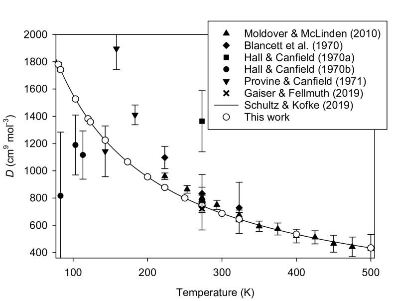
Figure 1: Comparison of calculated values of $D(T)$ for ⁴He with experimental resultsBlancett, Hall, and Canfield (1970); Hall and Canfield (1970a, b); Provine and Canfield (1971); Moldover and McLinden (2010); Gaiser and with correlation fitted to first-principles calculations by Schultz and Kofke.Schultz and Kofke (2019) Error bars represent expanded uncertainties with coverage factor $k=2$. Expanded uncertainties for this work are smaller than the size of the symbols; see Table 1.

In Fig. 1, our results from Table 1 are shown along with the experimental data for ⁴He. The data from the Burnett experiments of 50 years agoBlancett, Hall, and Canfield (1970); Hall and Canfield (1970a, b); Provine and Canfield (1971) are in qualitative agreement with our results, but are too scattered for meaningful quantitative comparison. The single dielectric-constant gas thermometry point of Gaiser and FellmuthGaiser and Fellmuth (2019); Gaiser has a relatively large uncertainty, but agrees well with our results. The results of Moldover and McLindenMoldover and McLinden (2010) are in excellent agreement with our calculations above about 300 K. At lower temperatures, there is a disagreement which is small but outside the mutual uncertainties. We note that the points of Moldover and McLinden that agree well are all from their “2007 isotherms,” while their points from the reanalyzed “2005 isotherms” measured by McLinden and Lösch-WillMcLinden and Lösch-Will (2007) show a systematic offset (a differing trend between the two sets was also noted by Shaul et al.Shaul et al. (2012)). This may suggest an unrecognized problem with the 2005 experiments. The 2007 isotherms were measured with new sinkers whose volumes were newly calibrated; it is plausible that there may have been a small error in calibration for the sinkers used in 2005.McLinden Figure 1 also shows the equation that Schultz and KofkeSchultz and Kofke (2019) fit to their results at 20 K and above, which were calculated using Boltzmann statistics only. It is not surprising that this equation is in excellent agreement with our results, since exchange effects are negligible at these temperatures.

V.3 Low-temperature behavior

Since one of the novel features of this work is the incorporation of exchange effects that become important at low temperature, in Figs. 2 and 3 we show low-temperature results for ⁴He and ³He, respectively. No low-temperature experimental data are available for comparison in either case.

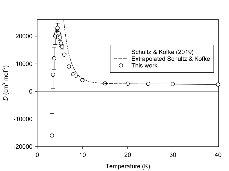
Figure 2: Calculated values of $D(T)$ for ⁴He at low temperatures. The correlation fitted to first-principles calculations by Schultz and KofkeSchultz and Kofke (2019) is extrapolated below 20 K. Error bars represent expanded uncertainties with coverage factor $k=2$, and are smaller than the symbol size at higher temperatures.

In Fig. 2, we see that $D(T)$ for ⁴He goes through a maximum near 4.5 K, turning sharply negative at the lowest temperatures (the three lowest temperatures in Table 1 are not plotted; they would be far below the bottom of the graph). We do not show the effect of exchange, since as discussed above the exchange contributions are relatively small compared to their uncertainty due to terms of opposite sign. The correlation that Schultz and KofkeSchultz and Kofke (2019) fitted to their Boltzmann results is in excellent agreement with the results obtained here down to its lower temperature limit of 20 K. It extrapolates well down to 15 K, but becomes increasingly inaccurate when extrapolated further.

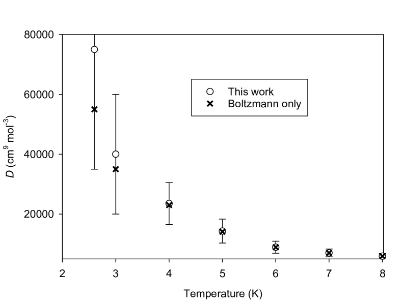
Figure 3: Calculated values of $D(T)$ for ³He at low temperatures, also showing results from Boltzmann statistics alone. Error bars represent expanded uncertainties with coverage factor $k=2$.

Figure 3 shows the low-temperature results for ³He. No maximum is evident in the temperature range investigated. We also show the values of $D(T)$ obtained when only Boltzmann statistics are considered. Incorporation of exchange effects is necessary for quantitative accuracy below roughly 4 K. The significant exchange effects on $D(T)$ for ³He, compared to a smaller effect for ⁴He due to competing terms, is similar to the behavior found in our previous work for $C(T)$.Garberoglio and Harvey (2011, 2020)

VI Conclusions

The values of $D(T)$ presented in Table 1 (for ⁴He) and Table 3 (for ³He) represent the first such values calculated from the current state-of-the-art pair and three-body potentials. They are also the first to include exchange effects, and the first to include complete uncertainty estimates. For ³He, Table 3 presents the first fully quantum calculations of $D(T)$.

Our ⁴He calculations at the level of Boltzmann statistics confirm previous calculations (with a slightly different two-body potential) from the group of Kofke.Shaul, Schultz, and Kofke (2012); Schultz and Kofke (2019) Because the two-body potential used in that workCencek et al. (2012) differs negligibly from the current state of the art for the purpose of calculating $D(T)$, we could consider those calculations to be additional data that supplement ours, making use of their somewhat smaller statistical uncertainties to improve our estimates of the Boltzmann contributions.

The exchange contributions to $D$ for ⁴He are relatively small, due to terms of opposite sign that mostly cancel each other. Because of this cancellation, our statistical uncertainty for the exchange contribution is similar in magnitude to the contribution itself. In contrast, for the fermion ³He, the exchange contributions all contribute in the positive direction, producing a significant effect on $D(T)$ at temperatures of roughly 4 K and below.

Several factors contribute to the uncertainty of the results. At low temperatures, the statistical uncertainty of the PIMC calculations is significant, not only in its own right but also in its contribution to the uncertainty $u_{V}(D)$ due to the uncertainty in the potential, which at the lowest temperatures is estimated by taking differences between PIMC calculations with shifted potentials. This could be somewhat improved with more computer resources, and also by employing some of the optimized methods for integrating virial coefficients developed by the group of Kofke.Shaul, Schultz, and Kofke (2012); Schultz and Kofke (2019)

Uncertainty due to imperfect knowledge of the potential cannot be reduced simply with more computer time; this aspect, which dominates the uncertainty at higher temperatures, requires careful development of potential-energy surfaces. The pair potential is now known with extraordinary accuracy;Czachorowski et al. (2020) further improvement may be desirable for other reasons but it will not reduce the uncertainty of virial coefficients beyond $B(T)$. The three-body potential has an estimated expanded ($k=2$) uncertainty of 2% at all configurations,Cencek, Patkowski, and Szalewicz (2009) which could be reduced somewhat with a concerted effort. Finally, the four-body potential is unknown, and is the largest uncertainty above roughly 10 K. Even an approximate four-body nonadditive potential, for example with a 20% uncertainty, would have a large impact on reducing the uncertainty of $D(T)$. The most important aspect of such a surface for metrology near room temperature would be its behavior at short-distance configurations dominated by repulsion, since those are the most important configurations at those temperatures. For use at cryogenic temperatures where the four-body uncertainty is still significant but the dispersion contribution is likely more important, its long-range behavior should approach that derived by Bade.Bade (1958)

Data Availability

The data that support the findings of this study are available within this article.

References

- Moldover et al. (2014) M. R. Moldover, R. M. Gavioso, J. B. Mehl, L. Pitre, M. de Podesta, and J. T. Zhang, “Acoustic gas thermometry,” Metrologia 51, R1–R19 (2014).
- Gaiser, Zandt, and Fellmuth (2015) C. Gaiser, T. Zandt, and B. Fellmuth, “Dielectric-constant gas thermometry,” Metrologia 52, S217–S226 (2015).
- Rourke et al. (2019) P. M. C. Rourke, C. Gaiser, B. Gao, D. Madonna Ripa, M. R. Moldover, L. Pitre, and R. J. Underwood, “Refractive-index gas thermometry,” Metrologia 56, 032001 (2019).
- Gaiser, Fellmuth, and Sabuga (2020) C. Gaiser, B. Fellmuth, and W. Sabuga, “Primary gas-pressure standard from electrical measurements and thermophysical ab initio calculations.” Nature Phys. 16, 177–180 (2020).
- Cencek et al. (2012) W. Cencek, M. Przybytek, J. Komasa, J. B. Mehl, B. Jeziorski, and K. Szalewicz, “Effects of adiabatic, relativistic, and quantum electrodynamics interactions on the pair potential and thermophysical properties of helium,” J. Chem. Phys. 136, 224303 (2012).
- Przybytek et al. (2017) M. Przybytek, W. Cencek, B. Jeziorski, and K. Szalewicz, “Pair potential with submillikelvin uncertainties and nonadiabatic treatment of the halo state of the helium dimer,” Phys. Rev. Lett. 119, 123401 (2017).
- Czachorowski et al. (2020) P. Czachorowski, M. Przybytek, M. Lesiuk, M. Puchalski, and B. Jeziorski, “Second virial coefficients for 4He and 3He from an accurate relativistic interaction potential,” Phys. Rev. A 102, 042810 (2020).
- Hirschfelder, Curtiss, and Bird (1954) J. O. Hirschfelder, C. F. Curtiss, and R. B. Bird, Molecular Theory of Gases and Liquids (John Wiley & Sons, New York, 1954).
- Garberoglio and Harvey (2011) G. Garberoglio and A. H. Harvey, “Path-integral calculation of the third virial coefficient of quantum gases at low temperatures,” J. Chem. Phys. 134, 134106 (2011).
- Garberoglio and Harvey (2020) G. Garberoglio and A. H. Harvey, “Erratum: Path-integral calculation of the third virial coefficient of quantum gases at low temperatures,” J. Chem. Phys. 152, 199903 (2020).
- Garberoglio, Moldover, and Harvey (2011) G. Garberoglio, M. R. Moldover, and A. H. Harvey, “Improved first-principles calculation of the third virial coefficient of helium,” J. Res. Natl. Inst. Stand. Technol. 116, 729–742 (2011).
- Garberoglio, Moldover, and Harvey (2020) G. Garberoglio, M. R. Moldover, and A. H. Harvey, “Erratum: Improved first-principles calculation of the third virial coefficient of helium,” J. Res. Natl. Inst. Stand. Technol. 125, 125019 (2020).
- Cencek, Patkowski, and Szalewicz (2009) W. Cencek, K. Patkowski, and K. Szalewicz, “Full-configuration-interaction calculation of three-body nonadditive contribution to helium interaction potential,” J. Chem. Phys. 131, 064105 (2009).
- Shaul, Schultz, and Kofke (2012) K. R. S. Shaul, A. J. Schultz, and D. A. Kofke, “Path-integral Mayer-sampling calculations of the quantum Boltzmann contribution to virial coefficients of helium-4,” J. Chem. Phys. 137, 184101 (2012).
- Schultz and Kofke (2019) A. J. Schultz and D. A. Kofke, “Virial coefficients of helium-4 from ab initio-based molecular models,” J. Chem. Eng. Data 64, 3742–3754 (2019).
- Gao et al. (2020) B. Gao, H. Zhang, D. Han, C. Pan, H. Chen, Y. Song, W. Liu, J. Hu, X. Kong, F. Sparasci, M. Plimmer, E. Luo, and L. Pitre, “Measurement of thermodynamic temperature between 5 K and 24.5 K with single-pressure refractive-index gas thermometry,” Metrologia 57, 065006 (2020).
- Garberoglio (2012) G. Garberoglio, “Quantum effects on virial coefficients: a numerical approach using centroids,” Chem. Phys. Lett. 525-526, 19–23 (2012).
- Hill (1987a) T. L. Hill, An Introduction to Statistical Thermodynamics (Dover, New York, 1987).
- Hill (1987b) T. L. Hill, Statistical Mechanics (Dover, New York, 1987).
- Boyd, Larsen, and Kilpatrick (1969) M. E. Boyd, S. Y. Larsen, and J. E. Kilpatrick, “Quantum mechanical second virial coefficient of a Lennard-Jones gas. Helium,” J. Chem. Phys. 50, 4034–4055 (1969).
- Lepage (1980) G. Lepage, “VEGAS: An adaptive multi-dimensional integration program,” Tech. Rep. (Cornell preprint CLNS 80-447, 1980).
- Kreckel (1997) R. Kreckel, “Parallelization of adaptive MC integrators,” Comput. Phys. Commun. 106, 258–266 (1997).
- Levy (1954) P. Levy, Memorial des Sciences Mathematiques (Gauthier Villars, Paris, 1954) fascicule 126.
- Jordan and Fosdick (1968) H. F. Jordan and L. D. Fosdick, “Three-particle effects in the pair distribution function for He4 gas,” Phys. Rev. 171, 128–149 (1968).
- Garberoglio and Harvey (2009) G. Garberoglio and A. H. Harvey, “First-principles calculation of the third virial coefficient of helium,” J. Res. Natl. Inst. Stand. Technol. 114, 249–262 (2009).
- Cencek et al. (2013) W. Cencek, G. Garberoglio, A. H. Harvey, M. O. McLinden, and K. Szalewicz, “Three-body nonadditive potential for argon with estimated uncertainties and third virial coefficient,” J. Phys. Chem. A 117, 7542–7552 (2013).
- Rodríguez-Cantano et al. (2016) R. Rodríguez-Cantano, R. Pérez de Tudela, M. Bartolomei, M. I. Hernández, J. Campos-Martínez, T. González-Lezana, P. Villarreal, J. Hernández-Rojas, and J. Bretón, “Examination of the Feynman–Hibbs approach in the study of NeN-coronene clusters at low temperatures,” J. Phys. Chem. A 120, 5370–5379 (2016).
- Bade (1957) W. L. Bade, “Drude-model calculation of dispersion forces. I. General theory,” J. Chem. Phys. 27, 1280–1284 (1957).
- Bade (1958) W. L. Bade, “Drude-model calculation of dispersion forces. III. The fourth-order contribution,” J. Chem. Phys. 28, 282–284 (1958).
- Wiebke, Pahl, and Schwerdtfeger (2012a) J. Wiebke, E. Pahl, and P. Schwerdtfeger, “Up to fourth virial coefficients from simple and efficient internal-coordinate sampling: Application to neon,” J. Chem. Phys. 137, 014508 (2012a).
- Wiebke, Pahl, and Schwerdtfeger (2012b) J. Wiebke, E. Pahl, and P. Schwerdtfeger, “Sensitivity of the thermal and acoustic virial coefficients of argon to the argon interaction potential,” J. Chem. Phys. 137, 064702 (2012b).
- Gaiser and Fellmuth (2018) C. Gaiser and B. Fellmuth, “Polarizability of helium, neon, and argon: New perspectives for gas metrology,” Phys. Rev. Lett. 120, 123203 (2018).
- Puchalski et al. (2020) M. Puchalski, K. Szalewicz, M. Lesiuk, and B. Jeziorski, “QED calculation of the dipole polarizability of helium atom,” Phys. Rev. A 101, 022505 (2020).
- Thakkar (1981) A. J. Thakkar, “The generator coordinate method applied to variational perturbation theory. Multipole polarizabilities, spectral sums, and dispersion coefficients for helium,” J. Chem. Phys. 75, 4496–4501 (1981).
- Blancett, Hall, and Canfield (1970) A. L. Blancett, K. R. Hall, and F. B. Canfield, “Isotherms for the He–Ar system at 50∘C, 0∘C and -50∘C up to 700 atm,” Physica 47, 75–91 (1970).
- Hall and Canfield (1970a) K. R. Hall and F. B. Canfield, “A least-squares method for reduction of Burnett data to compressibility factors and virial coefficients,” Physica 47, 99–108 (1970a).
- Hall and Canfield (1970b) K. R. Hall and F. B. Canfield, “Isotherms for the He–N2 system at -190∘C, -170∘C and -160∘C up to 700 atm,” Physica 47, 219–226 (1970b).
- Provine and Canfield (1971) J. A. Provine and F. B. Canfield, “Isotherms for the He–Ar system at -130, -115, and -90∘C up to 700 atm,” Physica 52, 79–91 (1971).
- McLinden and Lösch-Will (2007) M. O. McLinden and C. Lösch-Will, “Apparatus for wide-ranging, high-accuracy fluid () measurements based on a compact two-sinker densimeter,” J. Chem. Thermodyn. 39, 507–530 (2007).
- Moldover and McLinden (2010) M. R. Moldover and M. O. McLinden, “Using ab initio “data” to accurately determine the fourth density virial coefficient of helium,” J. Chem. Thermodyn. 42, 1193–1203 (2010).
- Gaiser and Fellmuth (2019) C. Gaiser and B. Fellmuth, “Highly-accurate density-virial-coefficient values for helium, neon, and argon at 0.01 ∘C determined by dielectric-constant gas thermometry,” J. Chem. Phys. 150, 134303 (2019).
- (42) C. Gaiser, Physikalisch-Technische Bundesanstalt, personal communication (2021).
- Shaul et al. (2012) K. R. S. Shaul, A. J. Schultz, D. A. Kofke, and M. R. Moldover, “Semiclassical fifth virial coefficients for improved ab initio helium-4 standards,” Chem. Phys. Lett. 531, 11–17 (2012).
- (44) M. O. McLinden, National Institute of Standards and Technology, personal communication (2020).