The moments of the distance between two random points
in a regular polygon

Abstract

In this paper, we derive formulas for the analytical calculation of the moments of the distance between two uniformly and independently distributed random points in an $n$-sided regular polygon. A number of closed form expressions is provided, e.g. the expected distances for $n=3,4,5,6,8,10,12$, where the results for $n=5,8,10,12$ are new to the best of the author’s knowledge. Applying results of Voss, remarkably short formulas for the second and the fourth moments are derived.
2010 Mathematics Subject Classification: 60D05, 52A22, 53C65
Keywords: Geometric probability, random distance, mean distance, moments of random distances, chord length distribution function, distance distribution function, regular polygons, chord power integrals

1 Introduction

Let $\mathcal{P}_{n,\;\!r}$, $n=3,4,\ldots$, be the regular polygon with $n$ sides and circumscribed circle with radius $r$. The distance between two points chosen independently and uniformly from $\mathcal{P}_{n,\;\!r}$ is a random variable, which we denote by $\varDelta_{n,\>\!r}$. The moments of $\varDelta_{n,\>\!r}$ are given by

$$M_{m}(\mathcal{P}_{n,\;\!r}):=\mathbb{E}[\varDelta_{n,\>\!r}^{m}]=\int_{0}^{d}x^{m}\,\mathrm{d}G_{n,\>\!r}(x)\,,$$

where $G_{n,\>\!r}$ is the cumulative distribution function of $\varDelta_{n,\>\!r}$, and $d$ is the diameter of $\mathcal{P}_{n,\;\!r}$. The first moment $M_{1}(\mathcal{P}_{n,\;\!r})$ is the mean distance between two (random) points in $\mathcal{P}_{n,\;\!r}$.

[10] found the mean values $M_{1}(\mathcal{P}_{3,\>\!r})$ (p. 206) and $M_{1}(\mathcal{P}_{4,\>\!r})$ (pp. 202-204, Problem XV) for the equilateral triangle and the square, respectively, in terms of the side length $a=2r\sin(\pi/n)$. (Czuber even found the mean distance in a rectangle. Concerning equilateral triangle, square and rectangle see also [27, p. 49].) [14] derived the distance distribution for a rectangle. [29] found the distribution function $G_{3,\>\!r}$ for the equilateral triangle in terms of the side length (see also [11]). The density function $g_{n,\>\!r}$ and the distribution function $G_{n,\>\!r}$ for any regular polygon were obtained by [5]. An example for the simulation of point distances is shown in Fig. 1.

[17] derived the distribution of the distance in a hypersphere. [4] studied the mean distance in the unit $n$-cube giving closed form expressions for the cases $n=1,\ldots,4$ (see also [8], especially Example 14). The density function of the distance between two points in a three-dimensional box was found by [24]. Furthermore, [25] found the density function for a 4-cube and a 5-cube.

Although the density function and the distribution function provide much more information than the mean value, there is a constant interest in mean values; see e. g. [12], and [9]. Recently, [7] obtained sharp inequalities for the mean distance in convex bodies.

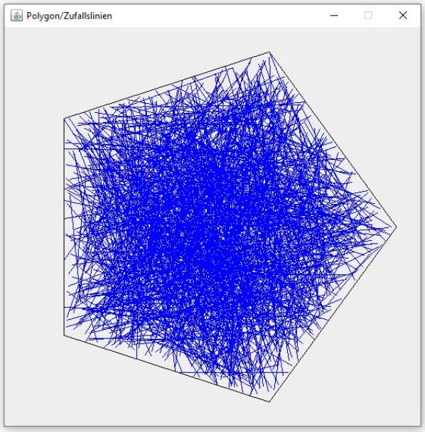
Fig. 1: Simulation of 1000 line segments each as a connection of two random points in $\mathcal{P}_{5,\>\!1}$ using PolygonV111.jar [1]
Here the empirical values of $M_{1}(\mathcal{P}_{5,\>\!1})$ and the variance $\mathrm{Var}[\varDelta_{5,\>\!1}]$ are 0.7911 (cf. Tab. 2) and 0.1316, respectively. Range: 1.6795

Without loss of generality one may assume that the centroid of $\mathcal{P}_{n,\;\!r}$ is located at the origin $O$ of a cartesian $x,y$-coordinate system, and the vertices of $\mathcal{P}_{n,\;\!r}$ are given by

$$X_{k}=x_{k}+\mathrm{i}y_{k}=r\mathrm{e}^{2\mathrm{i}k\alpha}\,,\quad k=0,1,\dots,n-1,$$ (1)

with angle

$$\alpha=\frac{1}{2}\>\measuredangle\left(\vv{OX_{0}},\vv{OX_{1}}\right)=\frac{\pi}{n}\,.$$

The distance $\ell_{k}$ between vertex $X_{0}$ and vertex $X_{k}$ is for $k=1,2,\ldots,n-1$ given by

$$\ell_{k}=r\,\sqrt{\left(\cos(2k\alpha)-1\right)^{2}+\sin^{2}(2k\alpha)}=2r\sin(k\alpha)\,.$$ (2)

Clearly, $\ell_{1}=2r\sin\alpha$ is the side length, and, denoting by $\lfloor\cdot\rfloor$ the integer part of $\,\cdot\,$,

$$d:=\ell_{K+1}\quad\mbox{with}\quad K:=\lfloor n/2\rfloor-1$$ (3)

is the diameter of $\mathcal{P}_{n,\;\!r}$. The length $L(\partial\>\!\mathcal{P}_{n,\;\!r})$ of the boundary $\partial\>\!\mathcal{P}_{n,\;\!r}$ and the area $A(\mathcal{P}_{n,\;\!r})$ of $\mathcal{P}_{n,\;\!r}$ are respectively

$$L(\partial\>\!\mathcal{P}_{n,\;\!r})=n\,\ell_{1}=2nr\sin\alpha\qquad\mbox{and}\qquad A(\mathcal{P}_{n,\;\!r})=n\,\frac{\ell_{1}}{2}\,r\cos\alpha=\frac{1}{2}\,nr^{2}\sin(2\alpha)\,.$$ (4)

For $\mathcal{P}_{n,\;\!r}$ with odd $n$ we denote by $\lambda$ the distance between the vertex $X_{0}$ and the side $\overline{X_{K+1}X_{K+2}}$,

$$\lambda=r+r\cos\alpha=2r\cos^{2}(\alpha/2)\,.$$ (5)

We will also use (5) for $\mathcal{P}_{n,\;\!r}$ with even $n$. Here $\lambda$ is the sum of $r=\left|\overline{OX_{0}}\right|$ and the distance between $O$ and side $\overline{X_{K}X_{K+1}}$ (and also $\overline{X_{K+1}X_{K+2}}$ ). For $\mathcal{P}_{n,\;\!r}$, $n=3,4,5,\ldots$, we have

$$\ell_{K}<\lambda<\ell_{K+1}=d\,.$$

The paper is organized as follows:

• In Section 2 we provide a simple and clear form of the chord length distribution function $F_{n,\>\!r}$ derived in [5]. This simple form is completely given in Theorem 1.

• For the point distance density function $g_{n,\>\!r}$ and the moments $M_{m}(\mathcal{P}_{n,\;\!r})$ required antiderivatives are provided in Section 3.

• From $F_{n,\>\!r}$ we conclude in Section 4 a simple and clear form of the point distance density function $g_{n,\>\!r}$ derived in [5].

• Formulas for analytically calculating the distance moments $M_{m}(\mathcal{P}_{n,\;\!r})$, $m=-1,0,1,2,\ldots$, are derived from $F_{n,\>\!r}$ in Section 5.

• Closed form expressions for the mean distances $M_{1}(\mathcal{P}_{n,\;\!r})$ and a number of further moments are given for $n=3,4,5,6,8,10,12$ in Section 6. According to the author’s knowledge, cases $n=5,8,10,12$ are new results.

• High precision values with respectively 75 and 76 digits for $M_{1}(\mathcal{P}_{n,\;\!r})/r$, $n=3,4,\ldots,30$, and $M_{m}(\mathcal{P}_{5,\>\!r})/r^{m}$, $m=-1,0,1,2,\ldots,10$, are given in Section 7.

• Using a result from [10], in Section 8 a short formula for the second moments $M_{2}(\mathcal{P}_{n,\;\!r})$ is derived. This makes it easier to calculate the variances $\mathrm{Var}[\varDelta_{n,\>\!r}]$. Especially in all cases, where a (short) closed form expression for the mean distance $M_{1}(\mathcal{P}_{n,\;\!r})$ is found, one has therefore also a closed form expression for the variance.

• Applying a result from [30], we obtain in Section 9 a short formula for the fourth moments $M_{4}(\mathcal{P}_{n,\;\!r})$. For this purpose it is used that the value of the second area moment of $\mathcal{P}_{n,\;\!r}$ with respect to an axis through the centroid of $\mathcal{P}_{n,\;\!r}$ is independent from the direction of this axis.

• Since clearly the moments for the circle $\mathcal{C}_{r}$ with radius $r$ are the limit values of the moments for $\mathcal{P}_{n,\;\!r}$ as $n$ tends to infinity, $\lim_{n\rightarrow\infty}M_{m}(\mathcal{P}_{n,\;\!r})=M_{m}(\mathcal{C}_{r})$, in Section 10 the already known moments are derived as values for comparison. (Comparisons have already been done in previous sections.)

• Finally, we point out the possibility of the simple derivation of chord power integrals for $\mathcal{P}_{n,\;\!r}$ from the present results (Section 11).

2 The chord length distribution function

A straight line $\mathfrak{g}$ in the plane is in Hesse normal form determined by the angle $\varphi$, $0\leq\varphi<2\pi$, between the positive $x$-axis and the direction perpendicular to $\mathfrak{g}$, and by its distance $p$, $0\leq p<\infty$, from the origin $O$,

$$\mathfrak{g}=\mathfrak{g}(p,\varphi)=\left\{(x,y)\in\mathbb{R}^{2}\colon x\cos\varphi+y\sin\varphi=p\right\}$$

(see [27, p. 2]). We assume $p$ and $\varphi$ to be independent random variables uniformly distributed in $[0,r]$ and $[0,2\pi)$, respectively, and consider only lines $\mathfrak{g}$ with $\mathfrak{g}\cap\mathcal{P}_{n,\;\!r}\neq\emptyset$. Such a line $\mathfrak{g}$ produces a chord of length $\varLambda_{n,\>\!r}$, $0\leq\varLambda_{n,\>\!r}\leq d=\ell_{K+1}$ (see (2), (3)). We denote by $F_{n,\>\!r}$ the distribution function of the random variable $\varLambda_{n,\>\!r}$, $F_{n,\>\!r}(x)=P(\varLambda_{n,\,r}\leq x)$.

Theorem 1.

With

$$\alpha=\pi/n\,,\qquad K=\lfloor n/2\rfloor-1\,,\qquad\ell_{k}=2r\sin(k\alpha)\,,\qquad\lambda=2r\cos^{2}(\alpha/2)\,,$$

$$h_{k}=2r\sin(k\alpha)\sin((k+1)\alpha)\,,\qquad p_{k}=\left\{\!\begin{array}[]{c@{\quad\mbox{if}\quad}l}0&n=3\,,\\[2.84544pt] \cot(2k\alpha)-\cot(2(k+1)\alpha)&n>3\,,\end{array}\right.$$

$$q_{k}=\tan(k\alpha)-\tan((k+1)\alpha)\,,\qquad s_{k}=\left\{\!\begin{array}[]{c@{\quad\mbox{if}\quad}l}1/2&n=3\,,\\[2.84544pt] k\,\alpha\,p_{k}&n>3\,,\end{array}\right.$$

$$\sigma_{\mu,\>\!a}(x)=x^{\mu}\arcsin\frac{a}{x}\,,\qquad\tau_{\mu,\>\!a}(x)=x^{\mu}\,\sqrt{x^{2}-a^{2}}\,,$$

the chord length distribution function $F_{n,\>\!r}$ of the regular polygon $\mathcal{P}_{n,\;\!r}$, $n=3,4,\ldots$, is given by

$$F_{n,\>\!r}(x)=P(\varLambda_{n,\,r}\leq x)=\left\{\begin{array}[]{c@{\quad\mbox{if}\quad}l}0&-\infty<x<\ell_{0}=0\,,\\[4.26773pt] 1-H_{k}(x)/\ell_{1}&\ell_{k}\leq x<\ell_{k+1}\;\;\mbox{for}\;\;k=0,\ldots,K,\\[4.26773pt] 1&\ell_{K+1}\leq x<\infty\end{array}\right.$$

with

$$H_{k}(x)=\left\{\begin{array}[]{ll}\ell_{1}-\left[1+\alpha\left(\tan\alpha-\cot\alpha\right)\right]x/2&\mbox{if}\quad k=0\,\wedge\,x<\lambda\,,\\[8.5359pt] p_{k}\,\sigma_{1,\>\!h_{k}}(x)-\left[k\alpha\cot(2k\alpha)-(k+1)\alpha\cot(2(k+1)\alpha)\right]x\\[4.26773pt] -\left(h_{k}\,p_{k}+2rq_{k}\cos\alpha\right)\tau_{-1,\>\!h_{k}}(x)&\mbox{if \, $(n$ is even $\,\wedge\,$ $1\leq k\leq K-1)$}\;\,\vee\\[4.26773pt] &\mbox{$(n$ is odd $\,\wedge\,$ $1\leq k\leq K$ $\,\wedge\,$ $x<\lambda)$}\,,\\[8.5359pt] \left[1/2-k\alpha\cot(2k\alpha)\right]x+\cot(2k\alpha)\,\sigma_{1,\>\!h_{k}}(x)-\left(h_{k}-2r\cos\alpha\right)h_{k}/x\\[4.26773pt] -\left[h_{k}\cot(2k\alpha)+2r\cos\alpha\tan(k\alpha)\right]\tau_{-1,\>\!h_{k}}(x)&\mbox{if}\quad\mbox{$n$ is even}\,\wedge\,k=K\,,\\[8.5359pt] p_{k}\,\sigma_{1,\>\!h_{k}}(x)+2\cot(2(k+1)\alpha)\,p_{k}\,\sigma_{1,\>\!\lambda}(x)-\left[(\pi-\alpha)\cot(2(k+1)\alpha)+s_{k}\right]x\\[4.26773pt] -\left(h_{k}\,p_{k}+2rq_{k}\cos\alpha\right)\tau_{-1,\>\!h_{k}}(x)-2\cos\alpha\,[2r\cos(\alpha/2)\sec((k+1)\alpha)\\[4.26773pt] -\,\lambda\csc(2(k+1)\alpha)]\,\tau_{-1,\>\!\lambda}(x)&\mbox{if}\quad\mbox{$n$ is odd}\,\wedge\,k=K\,\wedge\,x\geq\lambda\,.\end{array}\right.$$

Proof.

This is the chord length distribution function from [5, Theorem 1], simplified by inserting, rearranging and combining terms. Furthermore, the former case

$$(\mbox{$n$ is even}\,\wedge\,k\in\{0,\ldots,K-1\})\,\vee\,(\mbox{$n$ is odd}\,\wedge\,x<\lambda)$$

is split into two cases. ∎

Examples for graphs of distribution functions $F_{n,\>\!r}$ are shown in Fig. 2.

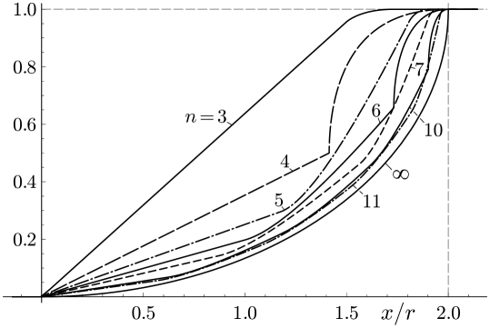
Fig. 2: Graphs of distribution functions $F_{n,\>\!r}$, $n=3$, $4$, $5$, $6$, $7$, $10$, $11$, and limit distribution function (circle)

3 Some antiderivatives

Lemma 1.

For $\mu=-1,0,1,2,\ldots$, an antiderivative $\widetilde{\psi}_{\mu,\>\!a}(x)$ of the function

$$\psi_{\mu,\>\!a}\colon[a,\infty)\>\rightarrow\>\mathbb{R}\,,\quad x\>\mapsto\>\psi_{\mu,\>\!a}(x):=\frac{x^{\mu}}{\sqrt{x^{2}-a^{2}}}\,,\quad a>0\,,$$

is given by

$$\widetilde{\psi}_{\mu,\>\!a}(x)=\left\{\begin{array}[]{lcl}\displaystyle{-\frac{1}{a}\arcsin\frac{a}{x}}&\mbox{if}&\mu=-1\,,\\[11.38092pt] \displaystyle{\ln\frac{x+\sqrt{x^{2}-a^{2}}}{a}}&\mbox{if}&\mu=0\,,\\[11.38092pt] \displaystyle{\frac{x^{\mu-1}\,\sqrt{x^{2}-a^{2}}\;\gamma_{\mu,\>\!a}(x)}{\mu}}&\mbox{if}&\mu=1,3,5,\ldots\,,\\[11.38092pt] \displaystyle{\frac{x^{\mu-1}\,\sqrt{x^{2}-a^{2}}\;\gamma_{\mu,\>\!a}(x)}{\mu}+\frac{(\mu-1)!!\,a^{\mu}}{\mu!!}\,\ln\frac{x+\sqrt{x^{2}-a^{2}}}{a}}&\mbox{if}&\mu=2,4,6,\ldots\,,\end{array}\right.$$

where

$$\gamma_{\mu,\>\!a}(x)=1+\sum_{\nu=1}^{\lfloor\frac{\mu-1}{2}\rfloor}\left(\frac{a}{x}\right)^{2\nu}\prod_{j=1}^{\nu}\frac{\mu+1-2j}{\mu-2j}\,.$$

Proof.

In the case $\mu=-1$ we have

$$\widetilde{\psi}_{-1,\>\!a}(x)=\int\frac{\mathrm{d}x}{x\,\sqrt{x^{2}-a^{2}}}=\int\frac{\mathrm{d}x}{x^{2}\,\sqrt{1-(a/x)^{2}}}\,.$$

The substitution $u=a/x$, $\mathrm{d}u=-a\,\mathrm{d}x/x^{2}$ gives

$$\widetilde{\psi}_{-1,\>\!a}(x)=-\frac{1}{a}\int\frac{\mathrm{d}u}{\sqrt{1-u^{2}}}=-\frac{1}{a}\arcsin u=-\frac{1}{a}\arcsin\frac{a}{x}\,.$$

For $\mu=0,1,2,\ldots$, the substitution

$$x=a\cosh u\,,\qquad\sqrt{x^{2}-a^{2}}=a\sinh u\,,\qquad\mathrm{d}x=a\sinh u\,\mathrm{d}u$$

yields

$$\widetilde{\psi}_{\mu,\>\!a}(x)=\int\frac{x^{\mu}}{\sqrt{x^{2}-a^{2}}}\,\mathrm{d}x=a^{\mu}\int\cosh^{\mu}u\,\mathrm{d}u\,.$$

For $\mu=0$ it follows that

$$\widetilde{\psi}_{0,\>\!a}(x)=\int\mathrm{d}u=u=\operatorname{arcosh}\frac{x}{a}=\ln\frac{x+\sqrt{x^{2}-a^{2}}}{a}\,.$$

For $\mu=1,3,5,\ldots$ from Eq. 2.412.4 in [16, Vol. 1, p. 127] we get

$$\int\cosh^{\mu}u\>\mathrm{d}u={} \frac{\sinh u}{\mu}\left[\cosh^{\mu-1}u+\sum_{\nu=1}^{\frac{\mu-1}{2}}\left(\prod_{j=1}^{\nu}\frac{\mu+1-2j}{\mu-2j}\right)\cosh^{\mu-1-2\nu}u\right]$$

$$={} \frac{\cosh^{\mu-1}u\,\sinh u}{\mu}\left(1+\sum_{\nu=1}^{\frac{\mu-1}{2}}\frac{1}{\cosh^{2\nu}u}\,\prod_{j=1}^{\nu}\frac{\mu+1-2j}{\mu-2j}\right),$$ (6)

whereas for $\mu=2,4,6\ldots$ from Eq. 2.412.1 in [16, Vol. 1, p. 127] we get

$$\int\cosh^{\mu}u\>\mathrm{d}u={} \frac{\cosh^{\mu-1}u\,\sinh u}{\mu}\left(1+\sum_{\nu=1}^{\frac{\mu}{2}-1}\frac{1}{\cosh^{2\nu}u}\,\prod_{j=1}^{\nu}\frac{\mu+1-2j}{\mu-2j}\right)+\frac{(\mu-1)!!}{\mu!!}\,u\,.$$ (7)

The back substitution

$$\cosh u=\frac{x}{a}\,,\quad\sinh u=\frac{\sqrt{x^{2}-a^{2}}}{a}\,,\quad u=\mathrm{arcosh}\,\frac{x}{a}=\ln\left(\frac{x}{a}+\sqrt{\left(\frac{x}{a}\right)^{2}-1}\,\right)$$

in (3) and (7) yields $\widetilde{\psi}_{\mu,\>\!a}(x)$ for the remaining cases in Lemma 1. ∎

Examples 1.

From Lemma 1 one gets the following special cases

$$\widetilde{\psi}_{1,\>\!a}(x)={} \sqrt{x^{2}-a^{2}}\,,$$

$$\widetilde{\psi}_{2,\>\!a}(x)={} \frac{1}{2}\left(x\,\sqrt{x^{2}-a^{2}}+a^{2}\ln\frac{x+\sqrt{x^{2}-a^{2}}}{a}\right),$$

$$\widetilde{\psi}_{3,\>\!a}(x)={} \frac{1}{3}\left(x^{2}+2a^{2}\right)\sqrt{x^{2}-a^{2}}\,,$$

$$\widetilde{\psi}_{4,\>\!a}(x)={} \frac{1}{8}\left[x\left(2x^{2}+3a^{2}\right)\sqrt{x^{2}-a^{2}}+3a^{4}\ln\frac{x+\sqrt{x^{2}-a^{2}}}{a}\right],$$

$$\widetilde{\psi}_{5,\>\!a}(x)={} \frac{1}{15}\left(3x^{4}+4a^{2}x^{2}+8a^{4}\right)\sqrt{x^{2}-a^{2}}\,,$$

$$\widetilde{\psi}_{6,\>\!a}(x)={} \frac{1}{48}\left[x\left(8x^{4}+10a^{2}x^{2}+15a^{4}\right)\sqrt{x^{2}-a^{2}}+15a^{6}\ln\frac{x+\sqrt{x^{2}-a^{2}}}{a}\right].$$

Remark 1.

The integral

$$\int\frac{x^{\mu-1}}{\sqrt{1-(a/x)^{2}}}\,\mathrm{d}x=\int\frac{x^{\mu}}{\sqrt{x^{2}-a^{2}}}\,\mathrm{d}x$$

is also used and discussed in the context of computing the moments of a point distance associated with triangles in [20, p. 4].

Lemma 2.

For $\mu=0,1,2,\ldots$, an antiderivative $\widetilde{\sigma}_{\mu,\>\!a}(x)$ of the function

$$\sigma_{\mu,\>\!a}\colon[a,\infty)\>\rightarrow\>\mathbb{R}\,,\quad x\>\mapsto\>\sigma_{\mu,\>\!a}(x):=x^{\mu}\arcsin\frac{a}{x}\,,\quad a\geq 0\,,$$

(from Theorem 1) is given by

$$\widetilde{\sigma}_{\mu,\>\!a}(x)=\left\{\begin{array}[]{ccl}\dfrac{1}{\mu+1}\left(x^{\mu+1}\arcsin\dfrac{a}{x}+a\,\widetilde{\psi}_{\mu,\>\!a}(x)\right)&\mbox{if}&a>0\,,\\[11.38092pt] 0&\mbox{if}&a=0\,,\end{array}\right.$$

with $\widetilde{\psi}_{\mu,\>\!a}(x)$ according to Lemma 1.

Proof.

Clearly, $\widetilde{\sigma}_{\mu,\>\!0}(x)\equiv 0$. If $a>0$, then integration by parts gives

$$\widetilde{\sigma}_{\mu,\>\!a}(x)=\int x^{\mu}\arcsin\frac{a}{x}\>\mathrm{d}x=\frac{1}{\mu+1}\left(x^{\mu+1}\arcsin\frac{a}{x}+a\,\widetilde{\psi}_{\mu,\>\!a}(x)\right).\qed$$

Lemma 3.

For $\mu=-1,0,1,2,\ldots$, an antiderivative $\widetilde{\tau}_{\mu,\>\!a}(x)$ of the function

$$\tau_{\mu,\>\!a}\colon[a,\infty)\>\rightarrow\>\mathbb{R}\,,\quad x\>\mapsto\>\tau_{\mu,\>\!a}(x):=x^{\mu}\,\sqrt{x^{2}-a^{2}}\,,\quad a\geq 0\,,$$

(from Theorem 1) is given by

$$\widetilde{\tau}_{\mu,\>\!a}(x)={} \left\{\begin{array}[]{ccl}\displaystyle{\frac{1}{\mu+2}\left(x^{\mu+1}\,\sqrt{x^{2}-a^{2}}-a^{2}\,\widetilde{\psi}_{\mu,\>\!a}(x)\right)}&\mbox{if}&a>0\,,\\[11.38092pt] \displaystyle{\frac{x^{\mu+2}}{\mu+2}}&\mbox{if}&a=0\,,\end{array}\right.$$

with $\widetilde{\psi}_{\mu,\>\!a}(x)$ according to Lemma 1.

Proof.

We have

$$\widetilde{\tau}_{\mu,\>\!0}(x)=\int x^{\mu+1}\,\mathrm{d}x=\frac{x^{\mu+2}}{\mu+2}\,.$$

In the case $a>0$ we have

$$\widetilde{\tau}_{\mu,\>\!a}(x)=\int x^{\mu}\,\sqrt{x^{2}-a^{2}}\,\mathrm{d}x=\int\frac{x^{\mu}\,(x^{2}-a^{2})}{\sqrt{x^{2}-a^{2}}}\,\mathrm{d}x=\int\frac{x^{\mu+2}}{\sqrt{x^{2}-a^{2}}}\,\mathrm{d}x-a^{2}\,\widetilde{\psi}_{\mu,\>\!a}(x)\,.$$ (8)

Integration by parts with

$$\begin{array}[]{c@{\:=\:}l@{\qquad}c@{\;=\;}l}u\hfil\>=\>&x^{\mu+1}\,,&v^{\prime}&\displaystyle{\frac{x}{\sqrt{x^{2}-a^{2}}}}\,,\\[9.95863pt] u^{\prime}\hfil\>=\>&(\mu+1)x^{\mu}\,,&v&\displaystyle{\sqrt{x^{2}-a^{2}}}\end{array}$$

yields

$$\int\frac{x^{\mu+2}}{\sqrt{x^{2}-a^{2}}}\,\mathrm{d}x={} x^{\mu+1}\,\sqrt{x^{2}-a^{2}}-(\mu+1)\int x^{\mu}\,\sqrt{x^{2}-a^{2}}\,\mathrm{d}x$$

$$={} x^{\mu+1}\,\sqrt{x^{2}-a^{2}}-(\mu+1)\,\widetilde{\tau}_{\mu,\>\!a}(x)\,.$$

Putting this into (8) provides

$$\widetilde{\tau}_{\mu,\>\!a}(x)=x^{\mu+1}\,\sqrt{x^{2}-a^{2}}-(\mu+1)\,\tau_{\mu,\>\!a}(x)-a^{2}\,\widetilde{\psi}_{\mu,\>\!a}(x)\,,$$

hence

$$\widetilde{\tau}_{\mu,\>\!a}(x)=\frac{1}{\mu+2}\left(x^{\mu+1}\,\sqrt{x^{2}-a^{2}}-a^{2}\,\widetilde{\psi}_{\mu,\>\!a}(x)\right).\qed$$

Remark 2.

I do not use $\widetilde{\tau}_{\mu,\>\!a}(x)$ in the closer form

$$\widetilde{\tau}_{\mu,\>\!a}(x)=\frac{1}{\mu+1}\left(x^{\mu+1}\,\sqrt{x^{2}-a^{2}}-\int\frac{x^{\mu+2}}{\sqrt{x^{2}-a^{2}}}\,\mathrm{d}x\right)=\frac{1}{\mu+1}\left(x^{\mu+1}\,\sqrt{x^{2}-a^{2}}-\widetilde{\psi}_{\mu+2,\>\!a}(x)\right),$$

which follows immediately by partial integration from the first integral in (8), because it does not hold for the case $\mu=-1$, which is also needed in the following.

4 The point distance density function

Theorem 2.

With $L(\partial\>\!\mathcal{P}_{n,\;\!r})$ and $A(\mathcal{P}_{n,\;\!r})$ according to (4), $\alpha$, $K$, $\ell_{k}$, $\lambda$, $h_{k}$, $p_{k}$, $q_{k}$, $s_{k}$ as in Theorem 1,

$$\widetilde{\sigma}_{1,\>\!a}(x)=\frac{1}{2}\left(x^{2}\arcsin\frac{a}{x}+a\,\sqrt{x^{2}-a^{2}}\right),\qquad\widetilde{\tau}_{-1,\>\!a}(x)=\sqrt{x^{2}-a^{2}}+a\arcsin\frac{a}{x}\,,$$

the density function $g_{n,\>\!r}$ of the distance $\varDelta_{n,\>\!r}$ between two uniformly and independently distributed random points in $\mathcal{P}_{n,\;\!r}$, $n=3,4,\ldots$, is given by

$$g_{n,\>\!r}(x)=\left\{\begin{array}[]{l@{\quad\mbox{if}\quad}l}\dfrac{2x}{A(\mathcal{P}_{n,\;\!r})}\left[\pi-\dfrac{L(\partial\>\!\mathcal{P}_{n,\;\!r})\,\phi^{\flat}(x)}{A(\mathcal{P}_{n,\;\!r})\,\ell_{1}}\right]&x\in[0,\ell_{K+1})\,,\\[14.22636pt] 0&x\in\mathbb{R}\setminus[0,\ell_{K+1})\,,\end{array}\right.$$

where

$$\phi^{\flat}(x)=\sum_{\nu=0}^{k-1}J_{\nu}^{\flat}(\ell_{\nu+1})+J_{k}^{\flat}(x)\quad\mbox{if}\quad\ell_{k}\leq x<\ell_{k+1}\,,\>\>k=0,\ldots,K$$

with

$$J_{k}^{\flat}(x)=\left\{\begin{array}[]{lcl}H_{0,\>\!k}^{\flat}(x)&\mbox{if}&k=0\,\wedge\,x<\lambda\,,\\[4.26773pt] H_{1,\>\!k}^{\flat}(x)-H_{1,\>\!k}^{\flat}(\ell_{k})&\mbox{if}&(\mbox{$n$ is even}\,\wedge\,1\leq k\leq K-1)\>\>\vee\\[1.42271pt] &&(\mbox{$n$ is odd}\,\wedge\,1\leq k\leq K\,\wedge\,x<\lambda)\,,\\[4.26773pt] H_{2,\>\!k}^{\flat}(x)-H_{2,\>\!k}^{\flat}(\ell_{k})&\mbox{if}&\mbox{$n$ is even}\,\wedge\,k=K\,,\\[4.26773pt] H_{3,\>\!k}^{\flat}(x)-H_{3,\>\!k}^{\flat}(\lambda)+H_{0,\>\!k}^{\flat}(\lambda)&\mbox{if}&n=3\,\wedge\,k=0\,\wedge\,x\geq\lambda\,,\\[4.26773pt] H_{3,\>\!k}^{\flat}(x)-H_{3,\>\!k}^{\flat}(\lambda)+H_{1,\>\!k}^{\flat}(\lambda)-H_{1,\>\!k}^{\flat}(\ell_{k})&\mbox{if}&\mbox{$n$ is odd}\,\wedge\,n>3\,\wedge\,x\geq\lambda\,,\end{array}\right.$$

and

$$H_{0,\>\!k}^{\flat}(x)={} \ell_{1}\,x-\left[1+\alpha\left(\tan\alpha-\cot\alpha\right)\right]x^{2}/4\,,$$

$$H_{1,\>\!k}^{\flat}(x)={} p_{k}\,\widetilde{\sigma}_{1,\>\!h_{k}}(x)-\left[k\alpha\cot(2k\alpha)-(k+1)\alpha\cot(2(k+1)\alpha)\right]x^{2}/2$$

$$-(h_{k}\,p_{k}+2rq_{k}\cos\alpha)\,\widetilde{\tau}_{-1,\>\!h_{k}}(x)\,,$$

$$H_{2,\>\!k}^{\flat}(x)={} \left[1/2-k\alpha\cot(2k\alpha)\right]x^{2}/2+\cot(2k\alpha)\,\widetilde{\sigma}_{1,\>\!h_{k}}(x)-\left(h_{k}-2r\cos\alpha\right)h_{k}\ln x$$

$$-\left[h_{k}\cot(2k\alpha)+2r\cos\alpha\tan(k\alpha)\right]\widetilde{\tau}_{-1,\>\!h_{k}}(x)\,,$$

$$H_{3,\>\!k}^{\flat}(x)={} p_{k}\,\widetilde{\sigma}_{1,\>\!h_{k}}(x)+2\cot(2(k+1)\alpha)\,\widetilde{\sigma}_{1,\>\!\lambda}(x)-\left[(\pi-\alpha)\cot(2(k+1)\alpha)+s_{k}\right]x^{2}/2$$

$$-(h_{k}\,p_{k}+2rq_{k}\cos\alpha)\,\widetilde{\tau}_{-1,\>\!h_{k}}(x)$$

$$-2\cos\alpha\left[2r\cos(\alpha/2)\sec((k+1)\alpha)-\lambda\csc(2(k+1)\alpha)\right]\widetilde{\tau}_{-1,\>\!\lambda}(x)\,.$$

Proof.

From Piefke’s [26, p. 130] result it immediately follows that the density functions $f_{n,\>\!r}$ and $g_{n,\>\!r}$ are connected by

$$g_{n,\>\!r}(x)=\frac{2L(\partial\>\!\mathcal{P}_{n,\;\!r})\,x}{A(\mathcal{P}_{n,\;\!r})^{2}}\int_{x}^{d}(s-x)f_{n,\>\!r}(s)\,\mathrm{d}s\,.$$

In [5] (see pp. 10-11) we concluded that

$$g_{n,\>\!r}(x)=\frac{2x}{A(\mathcal{P}_{n,\;\!r})}\left[\pi-\frac{L(\partial\>\!\mathcal{P}_{n,\;\!r})\,\phi^{\natural}(x)}{A(\mathcal{P}_{n,\;\!r})}\right]$$ (9)

where

$$\phi^{\natural}(x):=x-\int_{0}^{x}F_{n,\>\!r}(s)\,\mathrm{d}s=\int_{0}^{x}\left(1-F_{n,\>\!r}(s)\right)\mathrm{d}s\,.$$ (10)

So for $\ell_{k}\leq x\leq\ell_{k+1}$, $k=0,\dots,K$, we have

$$\ell_{1}\,\phi^{\natural}(x)=\phi^{\flat}(x):=\sum_{\nu=0}^{k-1}\,J_{\nu}^{\flat}(\ell_{\nu+1})+J_{k}^{\flat}(x)$$ (11)

where

$$J_{\nu}^{\flat}(x)=\int_{\ell_{\nu}}^{x}H_{\nu}(s)\,\mathrm{d}s$$ (12)

with $H_{\nu}$ according to Theorem 1 (the sum in (11) is empty if $k=0$). Considering the necessary case distinctions, the result of Theorem 2 follows from evaluating the integral (12) for $\nu=0,\ldots,K$. Note that the condition $k=0\,\wedge\,x<\lambda$ is an abbreviation for the equivalent, more detailed condition

$$(n=3\,\wedge\,k=0\leq x<\lambda)\,\vee\,(n>3\,\wedge\,k=0)\,.$$

The expression for $\widetilde{\sigma}_{1,\>\!a}(x)$ follows from Lemma 2 with $\widetilde{\psi}_{1,\>\!a}(x)$ in Examples 1, whereas the expression for $\widetilde{\tau}_{-1,\>\!a}(x)$ follows from Lemma 3 with $\widetilde{\psi}_{-1,\>\!a}(x)$ according to Lemma 1. ∎

Examples for graphs of density functions are shown in Figures 3 and 4. $f_{n,\>\!r}(x)=\mathrm{d}F_{n,\>\!r}(x)/\mathrm{d}x$ denotes the chord length density function.

Fig. 3: Graphs of density functions for $\mathcal{P}_{7,\>\!r}$: $r\times f_{7,\>\!r}(x)$, and $r\times g_{7,\>\!r}(x)$ (dashed)

Fig. 4: Graphs of density functions for $\mathcal{P}_{8,\>\!r}$: $r\times f_{8,\>\!r}(x)$, and $r\times g_{8,\>\!r}(x)$ (dashed)

5 Moments of the distance

Theorem 3.

With

• $L(\partial\>\!\mathcal{P}_{n,\;\!r})$, $A(\mathcal{P}_{n,\;\!r})$ according to (4),

• $\alpha$, $K$, $\ell_{k}$, $\lambda$, $h_{k}$, $p_{k}$, $q_{k}$, $s_{k}$ as in Theorem 1,

• $\widetilde{\sigma}_{\mu,\>\!a}(x)$ according to Lemma 2,

• $\widetilde{\tau}_{\mu,\>\!a}(x)$ according to Lemma 3,

the moments of the distance between two uniformly and independently distributed random points in $\mathcal{P}_{n,\;\!r}$ are given by

$$M_{m}(\mathcal{P}_{n,\;\!r})=\frac{2L(\partial\>\!\mathcal{P}_{n,\;\!r})}{(m+2)\,A(\mathcal{P}_{n,\;\!r})^{2}\,\ell_{1}}\,\sum_{k=0}^{K}\widetilde{J}_{m,\>\!k}(\ell_{k+1})\,,\quad m=-1,0,1,2,\ldots$$

where

$$\widetilde{J}_{m,\>\!k}(x)=\left\{\begin{array}[]{l@{\;\;\,}c@{\;\;\,}l}\widetilde{H}_{m,\>\!k}^{(0)}(x)&\mbox{if}&k=0\,\wedge\,x<\lambda\,,\\[5.69046pt] \widetilde{H}_{m,\>\!k}^{(1)}(x)-\widetilde{H}_{m,\>\!k}^{(1)}(\ell_{k})&\mbox{if}&\mbox{$(n$ is even $\,\wedge\,$ $1\leq k\leq K-1)$ $\,\vee$}\\ &&\mbox{$(n$ is odd $\,\wedge\,$ $1\leq k\leq K$ $\,\wedge\,$ $x<\lambda)$}\,,\\[5.69046pt] \widetilde{H}_{m,\>\!k}^{(2)}(x)-\widetilde{H}_{m,\>\!k}^{(2)}(\ell_{k})&\mbox{if}&\mbox{$n$ is even $\,\wedge\,$ $k=K$}\,,\\[5.69046pt] \widetilde{H}_{m,\>\!k}^{(3)}(x)-\widetilde{H}_{m,\>\!k}^{(3)}(\lambda)+\widetilde{H}_{m,\>\!k}^{(0)}(\lambda)&\mbox{if}&\mbox{$n=3$ $\,\wedge\,$ $k=0$ $\,\wedge\,$ $x\geq\lambda$}\,,\\[5.69046pt] \widetilde{H}_{m,\>\!k}^{(3)}(x)-\widetilde{H}_{m,\>\!k}^{(3)}(\lambda)+\widetilde{H}_{m,\>\!k}^{(1)}(\lambda)-\widetilde{H}_{m,\>\!k}^{(1)}(\ell_{k})&\mbox{if}&\mbox{$n$ is odd $\,\wedge\,$ $n>3$ $\,\wedge\,$ $x\geq\lambda$}\end{array}\right.$$

with

$$\widetilde{H}_{m,\>\!k}^{(0)}(x)={} \frac{\ell_{1}\,x^{m+3}}{m+3}-\frac{\left[1+\alpha\left(\tan\alpha-\cot\alpha\right)\right]x^{m+4}}{2(m+4)}\,,$$

$$\widetilde{H}_{m,\>\!k}^{(1)}(x)={} p_{k}\,\widetilde{\sigma}_{m+3,\>\!h_{k}}(x)-\left[k\alpha\cot(2k\alpha)-(k+1)\alpha\cot(2(k+1)\alpha)\right]\frac{x^{m+4}}{m+4}$$

$$-\left(h_{k}\,p_{k}+2rq_{k}\cos\alpha\right)\widetilde{\tau}_{m+1,\>\!h_{k}}(x)\,,$$

$$\widetilde{H}_{m,\>\!k}^{(2)}(x)={} \left(\frac{1}{2}-k\alpha\cot(2k\alpha)\right)\frac{x^{m+4}}{m+4}+\cot(2k\alpha)\,\widetilde{\sigma}_{m+3,\>\!h_{k}}(x)-\left(h_{k}-2r\cos\alpha\right)h_{k}\,\frac{x^{m+2}}{m+2}$$

$$-\left[h_{k}\cot(2k\alpha)+2r\cos\alpha\tan(k\alpha)\right]\widetilde{\tau}_{m+1,\>\!h_{k}}(x)\,,$$

$$\widetilde{H}_{m,\>\!k}^{(3)}(x)={} p_{k}\,\widetilde{\sigma}_{m+3,\>\!h_{k}}(x)+2\cot(2(k+1)\alpha)\,\widetilde{\sigma}_{m+3,\>\!\lambda}(x)$$

$$-\left[(\pi-\alpha)\cot(2(k+1)\alpha)+s_{k}\right]\frac{x^{m+4}}{m+4}-\left(h_{k}\,p_{k}+2rq_{k}\cos\alpha\right)\widetilde{\tau}_{m+1,\>\!h_{k}}(x)$$

$$-2\cos\alpha\left[2r\cos(\alpha/2)\sec((k+1)\alpha)-\lambda\csc(2(k+1)\alpha)\right]\widetilde{\tau}_{m+1,\>\!\lambda}(x)\,.$$

Proof.

From

$$M_{m}(\mathcal{P}_{n,\;\!r})=\mathbb{E}[\varDelta_{n,\>\!r}^{m}]=\int_{0}^{d}x^{m}\,g_{n,\>\!r}(x)\>\mathrm{d}x$$

with (9) and (10) we get

$$M_{m}(\mathcal{P}_{n,\;\!r})={} \frac{2\pi}{A(\mathcal{P}_{n,\;\!r})}\int_{0}^{d}x^{m+1}\,\mathrm{d}x-\frac{2L(\partial\>\!\mathcal{P}_{n,\;\!r})}{A(\mathcal{P}_{n,\;\!r})^{2}}\int_{x=0}^{d}x^{m+1}\int_{s=0}^{x}(1-F_{n,\>\!r}(s))\,\mathrm{d}s\,\mathrm{d}x$$

$$={} \frac{2\pi d^{m+2}}{(m+2)A(\mathcal{P}_{n,\;\!r})}-\frac{2L(\partial\>\!\mathcal{P}_{n,\;\!r})}{A(\mathcal{P}_{n,\;\!r})^{2}}\int_{x=0}^{d}x^{m+1}\int_{s=0}^{x}(1-F_{n,\>\!r}(s))\,\mathrm{d}s\,\mathrm{d}x\,.$$

Integration by parts with

$$\begin{array}[]{c@{\:=\:}l@{\qquad}c@{\:=\:}l}u\hfil\>=\>&\int_{0}^{x}(1-F(s))\,\mathrm{d}s\,,&v^{\prime}\hfil\>=\>&x^{m+1}\,,\\[7.11317pt] u^{\prime}\hfil\>=\>&1-F(x)\,,&v\hfil\>=\>&x^{m+2}/(m+2)\end{array}$$

yields

$$M_{m}(\mathcal{P}_{n,\;\!r})={} \frac{2\pi d^{m+2}}{(m+2)A(\mathcal{P}_{n,\;\!r})}-\frac{2L(\partial\>\!\mathcal{P}_{n,\;\!r})}{A(\mathcal{P}_{n,\;\!r})^{2}}\bigg{[}\left(\frac{x^{m+2}}{m+2}\,\int_{0}^{x}(1-F_{n,\>\!r}(s))\,\mathrm{d}s\right)\bigg{|}_{x=0}^{d}$$

$$-\frac{1}{m+2}\int_{0}^{d}x^{m+2}\,(1-F_{n,\>\!r}(x))\,\mathrm{d}x\bigg{]}$$

$$={} \frac{2\pi d^{m+2}}{(m+2)A(\mathcal{P}_{n,\;\!r})}-\frac{2L(\partial\>\!\mathcal{P}_{n,\;\!r})\,d^{m+2}}{(m+2)A(\mathcal{P}_{n,\;\!r})^{2}}\int_{0}^{d}(1-F_{n,\>\!r}(s))\,\mathrm{d}s$$

$$+\frac{2L(\partial\>\!\mathcal{P}_{n,\;\!r})}{(m+2)A(\mathcal{P}_{n,\;\!r})^{2}}\int_{0}^{d}x^{m+2}\,(1-F_{n,\>\!r}(x))\,\mathrm{d}x\,.$$

Now, integration by parts with

$$\begin{array}[]{c@{\:=\:}l@{\qquad}c@{\:=\:}l}u\hfil\>=\>&1-F_{n,\>\!r}(s)\,,&v^{\prime}\hfil\>=\>&1\,,\\[7.11317pt] u^{\prime}\hfil\>=\>&-f_{n,\>\!r}(s)\,,&v\hfil\>=\>&s\end{array}$$

gives

$$\int_{0}^{d}(1-F_{n,\>\!r}(s))\,\mathrm{d}s=\underbrace{s\,(1-F_{n,\>\!r}(s))\,\Big{|}_{0}^{d}}_{\displaystyle 0}\;\,+\,\underbrace{\int_{0}^{d}s\,f_{n,\>\!r}(s)\,\mathrm{d}s}_{\displaystyle\mathbb{E}[\varLambda_{n,\>\!r}]}\,.$$

With

$$\mathbb{E}[\varLambda_{n,\>\!r}]=\frac{\pi A(\mathcal{P}_{n,\;\!r})}{L(\partial\>\!\mathcal{P}_{n,\;\!r})}\qquad\mbox{\cite[cite]{[\@@bibref{}{Santalo}{}{}, p.\ 30]}}$$

we have found

$$M_{m}(\mathcal{P}_{n,\;\!r})=\frac{2L(\partial\>\!\mathcal{P}_{n,\;\!r})}{(m+2)A(\mathcal{P}_{n,\;\!r})^{2}}\int_{0}^{d}x^{m+2}\,(1-F_{n,\>\!r}(x))\,\mathrm{d}x\,.$$ (13)

It follows that

$$M_{m}(\mathcal{P}_{n,\;\!r})={} \frac{2L(\partial\>\!\mathcal{P}_{n,\;\!r})}{(m+2)A(\mathcal{P}_{n,\;\!r})^{2}}\,\sum_{k=0}^{K}\,\int_{\ell_{k}}^{\ell_{k+1}}x^{m+2}\,(1-F_{n,\>\!r}(x))\,\mathrm{d}x$$

$$={} \frac{2L(\partial\>\!\mathcal{P}_{n,\;\!r})}{(m+2)A(\mathcal{P}_{n,\;\!r})^{2}\,\ell_{1}}\,\sum_{k=0}^{K}\,\underbrace{\int_{\ell_{k}}^{\ell_{k+1}}x^{m+2}\,H_{k}(x)\,\mathrm{d}x}_{\displaystyle=:\widetilde{J}_{m,\>\!k}(\ell_{k+1})}.$$

with $H_{k}(x)$, $k\in\{0,1,\ldots,N\}$, from Theorem 1. So it remains to determine the antiderivatives

$$\widetilde{H}_{m,\>\!k}^{(q)}(x):=\int x^{m+2}\,H_{k}(x)\,\mathrm{d}x\,,$$

where the $q$ is used to indicate the necessary case distinctions.

The antiderivatives $\widetilde{\sigma}_{m+3,\>\!a}(x)$ and $\widetilde{\tau}_{m+1,\>\!a}(x)$ are used because of

$$\int x^{m+2}\,\sigma_{1,\>\!a}(x)\,\mathrm{d}x=\int x^{m+2}\,x\arcsin\frac{a}{x}\,\mathrm{d}x=\widetilde{\sigma}_{m+3,\>\!a}(x)$$

and

$$\int x^{m+2}\,\tau_{-1,\>\!a}(x)\,\mathrm{d}x=\int x^{m+2}\,\frac{\sqrt{x^{2}-a^{2}}}{x}\,\mathrm{d}x=\widetilde{\tau}_{m+1,\>\!a}(x)\,,$$

respectively. ∎

Remark 3.

Note that, although the expressions are in general quite long, Theorem 3 always provides closed form expressions for the moments of every $\mathcal{P}_{n,\;\!r}$.

Remark 4.

The relation (13) also follows from

$$T_{m}=\frac{2}{(m+2)(m+3)}\,S_{m+3}\,,\quad m=-1,0,1,2,\,\ldots,$$ (14)

where $S_{m}$ and $T_{m}$ are the $m$-th chord power integral and the $m$-th distance power integral, respectively ([6, pp. 19-20], [27, pp. 46-47], see also [28, p. 364, proof of Thm. 8.6.6; p. 374]). With

$$\mathbb{E}[\varLambda_{n,\>\!r}^{m}]=\frac{S_{m}(\mathcal{P}_{n,\;\!r})}{S_{0}(\mathcal{P}_{n,\;\!r})}=\frac{S_{m}(\mathcal{P}_{n,\;\!r})}{L(\partial\>\!\mathcal{P}_{n,\;\!r})}\quad\mbox{and}\quad M_{m}(\mathcal{P}_{n,\;\!r})=\mathbb{E}[\varDelta_{n,\>\!r}^{m}]=\frac{T_{m}(\mathcal{P}_{n,\;\!r})}{T_{0}(\mathcal{P}_{n,\;\!r})}=\frac{T_{m}(\mathcal{P}_{n,\;\!r})}{A(\mathcal{P}_{n,\;\!r})^{2}}$$ (15)

one gets

$$M_{m}(\mathcal{P}_{n,\;\!r})={} \frac{2}{(m+2)(m+3)}\,\frac{L(\partial\>\!\mathcal{P}_{n,\;\!r})}{A(\mathcal{P}_{n,\;\!r})^{2}}\int_{0}^{d}x^{m+3}\,\mathrm{d}F_{n,\>\!r}(x)$$

$$={} \frac{2L(\partial\>\!\mathcal{P}_{n,\;\!r})}{(m+2)A(\mathcal{P}_{n,\;\!r})^{2}}\int_{0}^{d}x^{m+2}\,(1-F_{n,\>\!r}(x))\,\mathrm{d}x$$

(see also [2, Eq. (2.3)]).

[18] derived a general formula for the second-order chord power integrals, $S_{2}$, for $\mathcal{P}_{n,\;\!r}$. This gives $T_{-1}$ and hence $\mathbb{E}[\Delta_{n,\>\!r}^{-1}]$ (see also Section 11).

Corollary 1.

The mean distance $M_{1}(\mathcal{P}_{n,\;\!r})$ between two uniformly and independently distributed random points in $\mathcal{P}_{n,\;\!r}$ is given by Theorem 3 with $m=1$. If $a>0$, then

$$\widetilde{\sigma}_{4,\>\!a}(x)={} \frac{1}{40}\left[8\,x^{5}\arcsin\frac{a}{x}+a\,x\left(2x^{2}+3a^{2}\right)\sqrt{x^{2}-a^{2}}+3\,a^{5}\ln\frac{x+\sqrt{x^{2}-a^{2}}}{a}\right],$$

$$\widetilde{\tau}_{2,\>\!a}(x)={} \frac{1}{8}\left[x\left(2x^{2}-a^{2}\right)\sqrt{x^{2}-a^{2}}-a^{4}\ln\frac{x+\sqrt{x^{2}-a^{2}}}{a}\right].$$

6 Examples of closed form expressions for the moments

For abbreviation we denote the moments in the following with $M_{m}$ instead of $M_{m}(\mathcal{P}_{n,\;\!r})$. From the context it will be clear for which polygon $\mathcal{P}_{n,\;\!r}$ the moments $M_{m}$ are valid.

•  3-gon (equilateral triangle)

$$\frac{M_{-1}}{r^{-1}}=\frac{4\sqrt{3}\ln 3}{3}\,,\quad\frac{M_{0}}{r^{0}}=1\,,\quad\frac{M_{1}}{r}=\frac{\sqrt{3}}{5}+\frac{3\sqrt{3}\ln 3}{20}\,,\quad\frac{M_{2}}{r^{2}}=\frac{1}{2}\,,$$

$$\frac{M_{3}}{r^{3}}=\frac{51\sqrt{3}}{280}+\frac{81\sqrt{3}\ln 3}{1120}\,,\quad\frac{M_{4}}{r^{4}}=\frac{9}{20}\,,\quad\frac{M_{5}}{r^{5}}=\frac{383\sqrt{3}}{1792}+\frac{405\sqrt{3}\ln 3}{7168}\,,\quad\frac{M_{6}}{r^{6}}=\frac{747}{1400}\,,$$

$$\frac{M_{7}}{r^{7}}=\frac{6669\sqrt{3}}{22528}+\frac{5103\sqrt{3}\ln 3}{90112}\,,\quad\frac{M_{8}}{r^{8}}=\frac{261}{350}\,,\quad$$

$$\frac{M_{9}}{r^{9}}=\frac{977913\sqrt{3}}{2129920}+\frac{1240029\sqrt{3}\ln 3}{18743296}\,,\quad\frac{M_{10}}{r^{10}}=\frac{2511}{2156}$$

With side length $\ell_{1}=\sqrt{3}\,r$ we have

$$\frac{M_{1}}{\ell_{1}}=\frac{1}{5}+\frac{3\ln 3}{20}=\frac{3}{5}\left(\frac{1}{3}+\frac{1}{4}\,\ln 3\right)\approx 0.36479184330021645371\,.$$

This result is due to [10, p. 206] (see also [27, p. 49], [32], [23], [34], and [2]).
•  4-gon (square)

$$\frac{M_{-1}}{r^{-1}}=-\frac{4}{3}+\frac{2\sqrt{2}}{3}+2\sqrt{2}\ln\left(1+\sqrt{2}\right)\,,\quad\frac{M_{0}}{r^{0}}=1\,,\quad\frac{M_{1}}{r}=\frac{2}{15}+\frac{2\sqrt{2}}{15}+\frac{\sqrt{2}\ln\left(1+\sqrt{2}\right)}{3}\,,$$

$$\frac{M_{2}}{r^{2}}=\frac{2}{3}\,,\quad\frac{M_{3}}{r^{3}}=\frac{34}{105}+\frac{8\sqrt{2}}{105}+\frac{\sqrt{2}\ln\left(1+\sqrt{2}\right)}{5}\,,\quad\frac{M_{4}}{r^{4}}=\frac{34}{45}\,,$$

$$\frac{M_{5}}{r^{5}}=\frac{73}{126}+\frac{4\sqrt{2}}{63}+\frac{5\sqrt{2}\ln\left(1+\sqrt{2}\right)}{28}\,,\quad\frac{M_{6}}{r^{6}}=\frac{116}{105}\,,$$

$$\frac{M_{7}}{r^{7}}=\frac{3239}{2970}+\frac{32\sqrt{2}}{495}+\frac{7\sqrt{2}\ln\left(1+\sqrt{2}\right)}{36}\,,\quad\frac{M_{8}}{r^{8}}=\frac{2992}{1575}\,,$$

$$\frac{M_{9}}{r^{9}}=\frac{1721}{780}+\frac{32\sqrt{2}}{429}+\frac{21\sqrt{2}\ln\left(1+\sqrt{2}\right)}{88}\,,\quad\frac{M_{10}}{r^{10}}=\frac{7648}{2079}$$

With side length $\ell_{1}=\sqrt{2}\,r$ we have

$$\frac{M_{1}}{\ell_{1}}=\frac{1}{15}\left[\sqrt{2}+2+5\,\ln\left(1+\sqrt{2}\right)\right]\approx 0.52140543316472067833\,.\\$$

This result is due to [10, pp. 202-204, Problem XV]. It can also be found in [14], [27, p. 49], [13, p. 479], [31], [22], and [2].
•  5-gon (pentagon)

$$\frac{M_{1}}{r}=\frac{\sqrt{2}}{480}\,\sqrt{5+\sqrt{5}}\left[24\sqrt{5}-8-\left(35+9\sqrt{5}\right)\ln 5-2\left(25+11\sqrt{5}\right)\ln\left(\sqrt{5}-2\right)\right],$$

$$\frac{M_{2}}{r^{2}}=\frac{7}{12}+\frac{\sqrt{5}}{12}\,,\quad\frac{M_{4}}{r^{4}}=\frac{47}{72}+\frac{11\sqrt{5}}{72}\,,\quad\frac{M_{6}}{r^{6}}=\frac{167}{168}+\frac{2\sqrt{5}}{7}\,,$$

$$\frac{M_{8}}{r^{8}}=\frac{65}{36}+\frac{145\sqrt{5}}{252}\,,\quad\frac{M_{10}}{r^{10}}=\frac{427375}{116424}+\frac{625\sqrt{5}}{504}$$

•  6-gon (hexagon)

$$\frac{M_{-1}}{r^{-1}}=-\frac{16}{9}+\frac{8}{3\sqrt{3}}+\frac{22\ln 3}{9}-\frac{4\ln\left(2+\sqrt{3}\right)}{9}\,,\quad\frac{M_{0}}{r^{0}}=1\,,$$

$$\frac{M_{1}}{r}=-\frac{7}{90}+\frac{7}{10\sqrt{3}}+\frac{19\ln 3}{40}-\frac{\ln\left(2+\sqrt{3}\right)}{60}\,,\quad\frac{M_{2}}{r^{2}}=\frac{5}{6}\,,$$

$$\frac{M_{3}}{r^{3}}=\frac{817}{5040}+\frac{117\sqrt{3}}{560}+\frac{867\ln 3}{2240}-\frac{3\ln\left(2+\sqrt{3}\right)}{1120}\,,\quad\frac{M_{4}}{r^{4}}=\frac{209}{180}\,,$$

$$\frac{M_{5}}{r^{5}}=\frac{146431}{290304}+\frac{963\sqrt{3}}{3584}+\frac{7045\ln 3}{14336}-\frac{5\ln\left(2+\sqrt{3}\right)}{7168}\,,\quad\frac{M_{6}}{r^{6}}=\frac{573}{280}\,,$$

$$\frac{M_{7}}{r^{7}}=\frac{7886969}{6082560}+\frac{8541\sqrt{3}}{20480}+\frac{139797\ln 3}{180224}-\frac{21\ln\left(2+\sqrt{3}\right)}{90112}\,,\quad\frac{M_{8}}{r^{8}}=\frac{13037}{3150}\,,$$

$$\frac{M_{9}}{r^{9}}=\frac{1395486403}{421724160}+\frac{34152111\sqrt{3}}{46858240}+\frac{52256421\ln 3}{37486592}-\frac{1701\ln\left(2+\sqrt{3}\right)}{18743296}\,,\quad\frac{M_{10}}{r^{10}}=\frac{76273}{8316}$$

The mean distance was obtained by [33] in the form

$$\frac{M_{1}}{\ell_{1}}=\frac{7\sqrt{3}}{30}-\frac{7}{90}+\frac{1}{60}\left[28\ln\left(2\sqrt{3}+3\right)+29\ln\left(2\sqrt{3}-3\right)\right]$$

with side length $\ell_{1}=r$. (Only the numerical approximation there is not correct.) [33] also derived the second moment.
•  8-gon (octagon)

$$\begin{aligned} \frac{M_{1}}{r}={}&\frac{4\sqrt{2}\,\pi}{3}+2\sqrt{2-\sqrt{2}}\left[\frac{1}{5}+\frac{13\sqrt{2}}{120}-\left(\frac{1}{20}+\frac{\sqrt{2}}{60}+\frac{2\pi}{3}\right)\sqrt{2+\sqrt{2}}\right.\\[1.42271pt] &-\frac{1}{48}\left(14+\frac{91\sqrt{2}}{10}\right)\ln\left(2+\sqrt{2}\right)+\frac{1}{48}\left(1+\frac{7\sqrt{2}}{10}\right)\ln\left(2-\sqrt{2}\right)\\[1.42271pt] &\left.+\,\frac{1}{20}\left(\frac{1}{3}-\frac{\sqrt{2}}{4}\right)\ln\left(2+\sqrt{2+\sqrt{2}}\,\right)+\frac{1}{40}\left(21+\frac{29\sqrt{2}}{2}\right)\ln\left(2+\sqrt{2-\sqrt{2}}\,\right)\right],\end{aligned}$$

$$\frac{M_{2}}{r^{2}}=\frac{2}{3}+\frac{\sqrt{2}}{6}\,,\quad\frac{M_{4}}{r^{4}}=\frac{77}{90}+\frac{16\sqrt{2}}{45}\,,\quad\frac{M_{6}}{r^{6}}=\frac{157}{105}+\frac{23\sqrt{2}}{30}\,,$$

$$\frac{M_{8}}{r^{8}}=\frac{326}{105}+\frac{928\sqrt{2}}{525}\,,\quad\frac{M_{10}}{r^{10}}=\frac{2132}{297}+\frac{3002\sqrt{2}}{693}$$

•  10-gon (decagon)

$$\begin{aligned} \frac{M_{1}}{r}={}&\frac{1}{600}\left[4\left(\sqrt{5125+2110\sqrt{5}}-24-11\sqrt{5}\right)-\left(505+239\sqrt{5}\right)\ln 2\right.\\[1.42271pt] &-30\left(4+3\sqrt{5}\right)\ln 5-\left(205+107\sqrt{5}\right)\ln\left(1+\sqrt{5}\right)\\[1.42271pt] &+\left(705+343\sqrt{5}\right)\ln\left(3+\sqrt{5}\right)-\left(105+47\sqrt{5}\right)\ln\left(\sqrt{5}+\sqrt{10+2\sqrt{5}}\,\right)\\[1.42271pt] &-\left(65-29\sqrt{5}\right)\ln\left(\sqrt{5}+\sqrt{10-2\sqrt{5}}\,\right)\\[1.42271pt] &\left.+\left(5+3\sqrt{5}\right)\ln\left(5-\sqrt{5}+2\sqrt{10-2\sqrt{5}}\,\right)\right],\end{aligned}$$

$$\frac{M_{2}}{r^{2}}=\frac{3}{4}+\frac{\sqrt{5}}{12}\,,\quad\frac{M_{4}}{r^{4}}=\frac{121}{120}+\frac{73\sqrt{5}}{360}\,,\quad\frac{M_{6}}{r^{6}}=\frac{1513}{840}+\frac{101\sqrt{5}}{210}\,,$$

$$\frac{M_{8}}{r^{8}}=\frac{23983}{6300}+\frac{1073\sqrt{5}}{900}\,,\quad\frac{M_{10}}{r^{10}}=\frac{149279}{16632}+\frac{223\sqrt{5}}{72}$$

•  12-gon (dodecagon)

$$\begin{aligned} \frac{M_{1}}{r}={}&\frac{1}{1080\sqrt{2}}\left[504-660\sqrt{2}+396\sqrt{3}-4\sqrt{6}+2\left(3+\sqrt{3}\right)\sqrt{2+\sqrt{3}}\right.\\[1.42271pt] &+6\left(1+47\sqrt{3}\right)\sqrt{2-\sqrt{3}}-\frac{27}{2}\left(15+11\sqrt{3}\right)\ln 3-4\left(27-\sqrt{3}\right)\ln\left(1+\sqrt{2}\right)\\[1.42271pt] &-4\sqrt{3}\ln\left(2+\sqrt{3}\right)+2\left(666+397\sqrt{3}\right)\ln\left(2-\sqrt{3}\right)\\[1.42271pt] &\left.-\left(33-19\sqrt{3}\right)\ln\left(2+\sqrt{2+\sqrt{3}}\,\right)+3\left(899+523\sqrt{3}\right)\ln\left(2+\sqrt{2-\sqrt{3}}\,\right)\right],\end{aligned}$$

$$\frac{M_{2}}{r^{2}}=\frac{2}{3}+\frac{1}{2\sqrt{3}}\,,\quad\frac{M_{4}}{r^{4}}=\frac{163}{180}+\frac{16}{15\sqrt{3}}\,,\quad\frac{M_{6}}{r^{6}}=\frac{71}{42}+\frac{661}{280\sqrt{3}}\,,$$

$$\frac{M_{8}}{r^{8}}=\frac{2357}{630}+\frac{424}{75\sqrt{3}}\,,\quad\frac{M_{10}}{r^{10}}=\frac{19099}{2079}+\frac{521}{36\sqrt{3}}$$

7 Numerical values

Numerical values for mean distances are given in Table 1; as an example, numerical values of moments for $\mathcal{P}_{5,\>\!r}$ may be found in Table 2. Using Mathematica, all of these values are obtained in two different ways:

• from the analytical solution in Theorem 3 together with Corollary 1,

• with numerical integration of

  $$M_{m}(\mathcal{P}_{n,\;\!r})=\int_{0}^{d}x^{m}g_{n,\>\!r}(x)\,\mathrm{d}x\,,\quad m=-1,0,1,2,\ldots,$$

  with the density function $g_{n,\>\!r}$ from Theorem 2.

The integration with NIntegrate required the use of WorkingPrecision and PrecisionGoal with suitable parameters and the splitting of the interval $[0,d]$ into subintervals corresponding to the different cases.

Fig. 5 shows how the expected distances converge against the expected distance for the circle $\mathcal{C}_{r}$ with radius $r$ (see (22), (23)).

Tab. 1: Numerical values for the mean distance

$n$	$M_{1}(\mathcal{P}_{n,\;\!r})/r$
13	0.631838006782679248439363765946266548228352566630216491351433566313728372374
14	0.737378635076566348769571883395005078909753124947971245022700482462877666826
15	0.793698195033753381760971632749605393899757772205869281310580089360628333136
16	0.826258949490232082314283750323326010149318430219325083679749121623475379023
17	0.846561326216093164027700615562504932765674717512492654162687095709688638441
18	0.860007978015497247289475476698227488793382581154266797596077525063820243821
19	0.869349677996368661272424554005308059692018424046355884971707394951786624055
10	0.876093016045821455437851478188806272714728045761204545124286721555684616290
11	0.881115231029789401140263676940968133233965295741220353166084636303706353850
12	0.884953782114214064113523711258487868874291600958495392058472857817523925124
13	0.887952286709934145445459685691276130847157335822373829281308109648830663248
14	0.890338490756764575735944950351064496029659712504470764018294183941844198540
15	0.892268061893522241535511225799568091834470923360328845899768230281232859177
16	0.893850267566140981445305963668775169957199844033103927893285119318229687792
17	0.895163602871345666236825912146252831958826216118785135695365798856133878291
18	0.896265616099618345601553161509629568460084862108878882774989021025191298962
19	0.897199265437573395493137709163413742006864641423080106927798068769440815162
20	0.897997136941287061624499349289436760861985366382141463318416018681802183354
21	0.898684307244840900050480580043224097039202683773713372510772133748302247016
22	0.899280326175269024941354083121964386591039853255838396881868160285060306349
23	0.899800615121290023756007063614270208943463748969153209258516013892113626863
24	0.900257469758660200325240434610054253924497221077824646172921619542988501865
25	0.900660789967557175495408085191424058901073528518182128993867898837236409609
26	0.901018618516579218784735836535111473157040513720977689621453066648252571482
27	0.901337543658947219455759999490321561595657334895730647458502404432253617671
28	0.901623003533134180530119238163701029410880699933247882599362042456633796468
29	0.901879518798576670046389739873503980147299817776988523533576670581933050086
30	0.902110872199677767358604753115452862213333195981189704602574660701374264234
$\infty$	0.905414787367226799040760964963637259573814873545707797320063112868390670986

Tab. 2: Numerical moments for $\mathcal{P}_{5,\>\!r}$

$m$	$M_{m}(\mathcal{P}_{5,\;\!r})/r^{m}$
$-1$	1.941532747349740237286829163767369291397446081205725687375578118779045940892
10	1.000000000000000000000000000000000000000000000000000000000000000000000000000
11	0.793698195033753381760971632749605393899757772205869281310580089360628333136
12	0.769672331458315808034097805727606352953384863300960477022574770450876743803
13	0.840599732769508183798403754882490669375942298135780251528211484773754115102
14	0.994399274340245648062512643833944980414538916051760874541387079159940696972
15	1.246445987635706663907926935585552909367630737102937503163072379765170177658
16	1.632924184047558960878811524399412257744938578936626397410732546307767883516
17	2.215335008390427051007858142854877211061180001285436481704877646702725059467
18	3.092181971180434547537024531611250214836863738665362023886032145176688627847
19	4.419361573049694692989749824140763338295447870581682927297936340850651262824
10	6.443751410804749342223892396954906260665664087034580725980990086289287076882

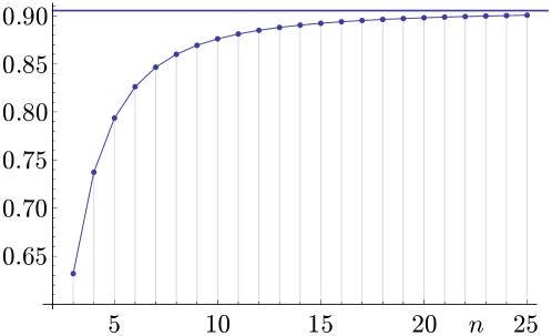
Fig. 5: $M_{1}(\mathcal{P}_{n,\;\!r})/r$, $n=3,4,\ldots,25$, and $M_{1}(\mathcal{C}_{r})/r$

8 Second moment and variance

Theorem 4.

The second moment of the point distance in $\mathcal{P}_{n,\;\!r}$, $r=3,4,\ldots$, is given by

$$M_{2}(\mathcal{P}_{n,\;\!r})=\frac{r^{2}}{3}\left(2+\cos\frac{2\pi}{n}\right).$$

Proof.

Due to [10, p. 217, Problem XXVII] we have

$$M_{2}(\mathcal{P}_{n,\;\!r})=\frac{2I_{p}(\mathcal{P}_{n,\;\!r})}{A(\mathcal{P}_{n,\;\!r})}$$ (16)

where $I_{p}(\mathcal{P}_{n,\;\!r})$ is the polar moment of area of $\mathcal{P}_{n,\;\!r}$ defined by

$$I_{p}(\mathcal{P}_{n,\;\!r})=\int_{\mathcal{P}_{n,\;\!r}}\left(x^{2}+y^{2}\right)\mathrm{d}A$$

whereby it is again assumed that the centroid of $\mathcal{P}_{n,\;\!r}$ is located at the origin $O$ of the $x,y$-coordinate system, and the vertex $X_{0}$ lies on the positive $x$-axis (see (1)). Now we rotate $\mathcal{P}_{n,\;\!r}$ about $O$ with angle $-\alpha$ so that the side $\overline{X_{0}X_{1}}$ is parallel to the $y$-axis. Using polar coordinates $\varphi$ and $\varrho$ we have $\varrho^{2}=x^{2}+y^{2}$ and $\mathrm{d}A=\varrho\,\mathrm{d}\varphi\,\mathrm{d}\varrho$, we get

$$I_{p}(\mathcal{P}_{n,\;\!r})=\int_{\varphi=0}^{2\pi}\int_{\varrho=0}^{R(\varphi)}\varrho^{3}\,\mathrm{d}\varrho\,\mathrm{d}\varphi$$

where $R(\varphi)$ is the equation of $\partial\>\!\mathcal{P}_{n,\;\!r}$, and further

$$I_{p}(\mathcal{P}_{n,\;\!r})={} 2n\int_{\varphi=0}^{\pi/n}\mathrm{d}\varphi\int_{\varrho=0}^{R(\varphi)}\varrho^{3}\,\mathrm{d}\varrho=\frac{n}{2}\int_{\varphi=0}^{\pi/n}R(\varphi)^{4}\,\mathrm{d}\varphi$$

$$={} \frac{nr^{4}}{2}\cos^{4}(\pi/n)\int_{\varphi=0}^{\pi/n}\left(1+\tan^{2}\varphi\right)^{2}\mathrm{d}\varphi$$

$$={} \frac{nr^{4}}{2}\cos^{4}(\pi/n)\int_{\varphi=0}^{\pi/n}\frac{\mathrm{d}\varphi}{\cos^{4}\varphi}\,.$$

With Eq. 2.526.12 in [16, Vol. 1, p. 173] we get

$$I_{p}(\mathcal{P}_{n,\;\!r})={} \frac{nr^{4}}{2}\cos^{4}(\pi/n)\left(\frac{\sin(\pi/n)}{3\cos^{3}(\pi/n)}+\frac{2}{3}\tan(\pi/n)\right)$$

$$={} \frac{nr^{4}}{6}\cos^{4}(\pi/n)\,\frac{\sin(\pi/n)+2\sin(\pi/n)\cos^{2}(\pi/n)}{\cos^{3}(\pi/n)}$$

$$={} \frac{nr^{4}}{6}\cos(\pi/n)\sin(\pi/n)\left[1+2\cos^{2}(\pi/n)\right]$$

$$={} \frac{nr^{4}}{6}\cos(\pi/n)\sin(\pi/n)\left[2+\cos(2\pi/n)\right].$$ (17)

Now from (16) with the area

$$A(\mathcal{P}_{n,\;\!r})=nr^{2}\cos(\pi/n)\sin(\pi/n)$$ (18)

(see also (4)) it follows that

$$M_{2}(\mathcal{P}_{n,\;\!r})=\frac{r^{2}}{3}\left(2+\cos\frac{2\pi}{n}\right).\qed$$

Remark 5.

We get

$$\lim_{n\rightarrow\infty}M_{2}(\mathcal{P}_{n,\;\!r})=\frac{r^{2}}{3}\,(2+1)=r^{2}$$

which is the result for the circle with radius $r$ (see Table 3).

Corollary 2.

The variance of the distance $\varDelta_{n,\,r}$ between two random points in a regular polygon is given by

$$\mathrm{Var}[\varDelta_{n,\,r}]=\mathbb{E}\big{[}\varDelta_{n,\,r}^{2}\big{]}-\mathbb{E}[\varDelta_{n,\,r}]^{2}=M_{2}(\mathcal{P}_{n,\;\!r})-M_{1}(\mathcal{P}_{n,\;\!r})^{2}$$

with $M_{1}(\mathcal{P}_{n,\;\!r})$ according to Corollary 1, and $M_{2}(\mathcal{P}_{n,\;\!r})$ according to Theorem 4.

Fig. 6 shows how the variances converge against the variance for the circle $\mathcal{C}_{r}$ with radius $r$ (see (25)).

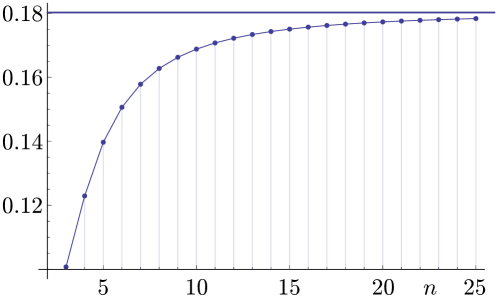
Fig. 6: $\mathrm{Var}[\varDelta_{n,\>\!r}]/r^{2}$, $n=3,4,\ldots,25$, and $\mathrm{Var}[\varDelta_{r}]/r^{2}$

9 Fourth moment

Theorem 5.

The fourth moment of the point distance in $\mathcal{P}_{n,\;\!r}$, $r=3,4,\ldots$, is given by

$$M_{4}(\mathcal{P}_{n,\;\!r})=\frac{r^{4}}{90}\left(77+64\cos\frac{2\pi}{n}+9\cos\frac{4\pi}{n}\right).$$

Proof.

From (14) together with the second formula in (15) we get

$$M_{4}(\mathcal{P}_{n,\;\!r})=\frac{S_{7}(\mathcal{P}_{n,\;\!r})}{21A(\mathcal{P}_{n,\;\!r})^{2}}\,.$$

According to [30, Eq. (16)] we can compute $S_{7}$ with

$$S_{7}(\mathcal{P}_{n,\;\!r})=42\left[A(\mathcal{P}_{n,\;\!r})I_{p}^{(4)}(\mathcal{P}_{n,\;\!r})+I_{p}(\mathcal{P}_{n,\;\!r})^{2}+2\left(I_{x}(\mathcal{P}_{n,\;\!r})^{2}+I_{y}(\mathcal{P}_{n,\;\!r})^{2}\right)\right]$$

where

$$I_{p}^{(4)}(\mathcal{P}_{n,\;\!r})=\int_{\mathcal{P}_{n,\;\!r}}\left(x^{2}+y^{2}\right)^{2}\mathrm{d}A=\frac{1}{6}\int_{0}^{2\pi}R(\varphi)^{6}\,\mathrm{d}\varphi\,,$$

$$I_{x}(\mathcal{P}_{n,\;\!r})=\int_{\mathcal{P}_{n,\;\!r}}y^{2}\,\mathrm{d}A\,,\qquad I_{y}(\mathcal{P}_{n,\;\!r})=\int_{\mathcal{P}_{n,\;\!r}}x^{2}\,\mathrm{d}A$$

whereby the centroid of $\mathcal{P}_{n,\;\!r}$ is located at the origin $O$ of the $x,y$-coordinate system and the axes are the principal axes of intertia. ($I_{x}$ und $I_{y}$ are the second moments of area with respect to the $x$-axis and the $y$-axis, respectively.) So we have

$$M_{4}(\mathcal{P}_{n,\;\!r})=\frac{2I_{p}^{(4)}(\mathcal{P}_{n,\;\!r})}{A(\mathcal{P}_{n,\;\!r})}+\frac{2I_{p}(\mathcal{P}_{n,\;\!r})^{2}}{A(\mathcal{P}_{n,\;\!r})^{2}}+\frac{4\left(I_{x}(\mathcal{P}_{n,\;\!r})^{2}+I_{y}(\mathcal{P}_{n,\;\!r})^{2}\right)}{A(\mathcal{P}_{n,\;\!r})^{2}}\,.$$ (19)

We get

$$I_{p}^{(4)}(\mathcal{P}_{n,\;\!r})={} \frac{n}{3}\int_{0}^{\pi/n}R(\varphi)^{6}\,\mathrm{d}\varphi=\frac{nr^{6}}{3}\cos^{6}(\pi/n)\int_{0}^{\pi/n}\left(1+\tan^{2}\varphi\right)^{3}\mathrm{d}\varphi$$

$$={} \frac{nr^{6}}{3}\cos^{6}(\pi/n)\int_{0}^{\pi/n}\frac{\mathrm{d}\varphi}{\cos^{6}\varphi}\,,$$

and, with Eq. 2.526.14 in [16, Vol. 1, p. 174],

$$I_{p}^{(4)}(\mathcal{P}_{n,\;\!r})={} \frac{nr^{6}}{3}\cos^{6}(\pi/n)\left(\frac{\sin(\pi/n)}{5\cos^{5}(\pi/n)}+\frac{4}{15}\tan^{3}(\pi/n)+\frac{4}{5}\tan(\pi/n)\right)$$

$$={} \frac{nr^{6}}{45}\cos(\pi/n)\sin(\pi/n)\left[3+4\sin^{2}(\pi/n)\cos^{2}(\pi/n)+12\cos^{4}(\pi/n)\right]$$

$$={} \frac{nr^{6}}{45}\cos(\pi/n)\sin(\pi/n)\left[8+6\cos(2\pi/n)+\cos(4\pi/n)\right],$$

and, with the area (18),

$$\frac{2I_{p}^{(4)}(\mathcal{P}_{n,\;\!r})}{A(\mathcal{P}_{n,\;\!r})}=\frac{2r^{4}}{45}\left[8+6\,\cos(2\pi/n)+\cos(4\pi/n)\right].$$ (20)

With (8) we get

$$\frac{2I_{p}(\mathcal{P}_{n,\;\!r})^{2}}{A(\mathcal{P}_{n,\;\!r})^{2}}={} 2\,\frac{\left[\frac{1}{6}nr^{4}\cos(\pi/n)\sin(\pi/n)\,\left(2+\cos(2\pi/n)\right)\right]^{2}}{(nr^{2}\cos(\pi/n)\sin(\pi/n))^{2}}=\frac{r^{4}}{18}\left[2+\cos(2\pi/n)\right]^{2}$$

$$={} \frac{r^{4}}{36}\left[9+8\cos(2\pi/n)+\cos(4\pi/n)\right].$$ (21)

Now we compute $I_{x}(\mathcal{P}_{n,\;\!r})$ and $I_{y}(\mathcal{P}_{n,\;\!r})$. Since the axes of the coordinate system are principal axes of inertia and the origin is located in the centroid of $\mathcal{P}_{n,\;\!r}$, the second area moments $I_{x}(\mathcal{P}_{n,\;\!r})$ and $I_{y}(\mathcal{P}_{n,\;\!r})$ take extreme values compared to all other second area moments with respect to axes through the centroid [15, p. 165]. This means that one of the two values $I_{x}(\mathcal{P}_{n,\;\!r})$ and $I_{y}(\mathcal{P}_{n,\;\!r})$ is the maximum and one is the minimum value. An axis of symmetry and the axis perpendicular to it are always principal axes of inertia [15, p. 165]. Each polygon $\mathcal{P}_{n,\;\!r}$, $n=3,4,\ldots$, has more than two symmetry axes that are not perpendicular to each other. Therefore it follows that the second area moment is equal for all axes through the centroid. Thus with $I_{x}(\mathcal{P}_{n,\;\!r})+I_{y}(\mathcal{P}_{n,\;\!r})=I_{p}(\mathcal{P}_{n,\;\!r})$ we have found

$$I_{x}(\mathcal{P}_{n,\;\!r})=I_{y}(\mathcal{P}_{n,\;\!r})=\frac{1}{2}\,I_{p}(\mathcal{P}_{n,\;\!r})\,,$$

hence

$$\frac{4\left(I_{x}(\mathcal{P}_{n,\;\!r})^{2}+I_{y}(\mathcal{P}_{n,\;\!r})^{2}\right)}{A(\mathcal{P}_{n,\;\!r})^{2}}=\frac{2I_{p}(\mathcal{P}_{n,\;\!r})^{2}}{A(\mathcal{P}_{n,\;\!r})^{2}}\,,$$

and (19) becomes

$$M_{4}(\mathcal{P}_{n,\;\!r})=\frac{2I_{p}^{(4)}(\mathcal{P}_{n,\;\!r})}{A(\mathcal{P}_{n,\;\!r})}+\frac{4I_{p}(\mathcal{P}_{n,\;\!r})^{2}}{A(\mathcal{P}_{n,\;\!r})^{2}}$$

(cp. Eq. (17) in [30]). So, with (20) and (9) we finally get

$$M_{4}(\mathcal{P}_{n,\;\!r})={} \frac{2r^{4}}{45}\left[8+6\,\cos(2\pi/n)+\cos(4\pi/n)\right]+\frac{r^{4}}{18}\left[9+8\cos(2\pi/n)+\cos(4\pi/n)\right]$$

$$={} \frac{r^{4}}{90}\left(77+64\cos\frac{2\pi}{n}+9\cos\frac{4\pi}{n}\right).\qed$$

Remark 6.

From Theorem 5 we get

$$\lim_{n\rightarrow\infty}M_{4}(\mathcal{P}_{n,\;\!r})=\frac{r^{4}}{90}\,(77+64+9)=\frac{5}{3}\,r^{4}$$

which is the result for the circle with radius $r$ (see Table 3).

Remark 7.

With the side length $\ell_{1}=2r\sin(\pi/n)$ and the area $A(\mathcal{P}_{n,\;\!r})$ (see (18)), the second area moment $I_{x}(\mathcal{P}_{n,\;\!r})$ with respect to an axis through the centroid of $\mathcal{P}_{n,\;\!r}$ can be written in the form

$$I_{x}(\mathcal{P}_{n,\;\!r})=\frac{A(\mathcal{P}_{n,\;\!r})}{12}\left(3r^{2}-\frac{\ell_{1}^{2}}{2}\right).$$

This result can already be found in [19, p. 249]. The independence of $I_{x}(\mathcal{P}_{n,\;\!r})$ from the direction of the $x$-axis through the centroid is also discussed in [3].

10 Circle

Now, we consider the moments $M_{m}(\mathcal{C}_{r})$, $m=1,2,\ldots$, of the distance $\varDelta_{r}$ between two random points in a circle $\mathcal{C}_{r}$ with radius $r$.

[10] found

$$M_{1}(\mathcal{C}_{r})=\frac{128}{45\pi}\,r\quad\mbox{(p.\ 197)}\,,\qquad M_{2}(\mathcal{C}_{r})=r^{2}\quad\mbox{(p.\ 217)}\,.$$ (22)

A numerical approximation of $M_{1}(\mathcal{C}_{r})$ is given by

$$M_{1}(\mathcal{C}_{r})\approx 0.90541478736722679904\,r\,.$$ (23)

A general formula for $M_{m}(\mathcal{C}_{r})$ can be found in [21, p. 207, Theorem 2.3.15]. Here we calculate the moments using (13), with $\mathcal{C}_{r}$ instead of $\mathcal{P}_{n,\;\!r}$, and $2r$ instead of $d$, in the form

$$M_{m}(\mathcal{C}_{r})=\mathbb{E}[\varDelta_{r}^{m}]=\frac{2L(\partial\>\!\mathcal{C}_{r})}{(m+2)A(\mathcal{C}_{r})^{2}}\int_{0}^{2r}x^{m+2}\left(1-F_{r}(x)\right)\mathrm{d}x$$

where $F_{r}(x)$ is the chord length distribution function of $\mathcal{C}_{r}$. One easily finds

$$F_{r}(x)=1-\sqrt{1-\left(\frac{x}{2r}\right)^{2}}$$

(see also [26]), hence

$$M_{m}(\mathcal{C}_{r})=\frac{4\pi r}{(m+2)\pi^{2}r^{4}}\int_{0}^{2r}x^{m+2}\,\sqrt{1-\left(\frac{x}{2r}\right)^{2}}\,\mathrm{d}x\,.$$

The substitution

$$t=\left(\frac{x}{2r}\right)^{2}$$

yields

$$M_{m}(\mathcal{C}_{r})=\frac{2^{m+4}\,r^{m}}{(m+2)\pi}\int_{0}^{1}t^{(m+1)/2}\,(1-t)^{1/2}\,\mathrm{d}t\,.$$

The last integral is the Euler beta function $B((m+3)/2,3/2)$. Using the relationship to the gamma function $\varGamma$,

$$B(x,y)=\frac{\varGamma(x)\varGamma(y)}{\varGamma(x+y)}\,,$$

and $\varGamma(1/2)=\sqrt{\pi}$ one finds

$$M_{m}(\mathcal{C}_{r})=\frac{2^{m+4}\,r^{m}}{\sqrt{\pi}\,(m+2)(m+4)}\,\frac{\varGamma\!\left(\frac{m+3}{2}\right)}{\varGamma\!\left(\frac{m}{2}+2\right)}\,.$$ (24)

This is Mathai’s result. Special values of (24) are to be found in Table 3 .

Tab. 3: Special values of $M_{m}(\mathcal{C}_{r})$

$m$	1	2	3	4	5	6	7	8
$M_{m}(\mathcal{C}_{r})$	$\dfrac{128}{45\pi}\,r$	$r^{2}$	$\dfrac{2048}{525\pi}\,r^{3}$	$\dfrac{5}{3}\,r^{4}$	$\dfrac{16384}{2205\pi}\,r^{5}$	$\dfrac{7}{2}\,r^{6}$	$\dfrac{524288}{31185\pi}\,r^{7}$	$\dfrac{42}{5}\,r^{8}$
Eq.	(22)	(22)

For the variance we have

$$\mathrm{Var}[\varDelta_{r}]={} \mathbb{E}\big{[}\varDelta_{r}^{2}\big{]}-\mathbb{E}[\varDelta_{r}]^{2}=M_{2}(\mathcal{C}_{r})-M_{1}(\mathcal{C}_{r})^{2}=\left[1-\left(\frac{128}{45\pi}\right)^{\!2}\right]r^{2}$$ (25)

$$\approx{} 0.18022406281675948280\,r^{2}\,.$$

11 Chord power integrals

From (14) with the second formula in (15) one gets

$$S_{m}(\mathcal{P}_{n,\;\!r})=\frac{m(m-1)}{2}\,T_{m-3}(\mathcal{P}_{n,\;\!r})=\frac{m(m-1)}{2}\,A(\mathcal{P}_{n,\;\!r})^{2}\,M_{m-3}(\mathcal{P}_{n,\;\!r})\,,\quad m=2,3,4,\ldots,$$

(see also [27, p. 47]). Thus it is easy to compute chord power integrals $S_{m}(\mathcal{P}_{n,\;\!r})$ with the results of the present paper. One obtains e.g. for the second chord power integral of $\mathcal{P}_{6,\>\!r}$

$$S_{2}(\mathcal{P}_{6,\>\!r})=A(\mathcal{P}_{6,\>\!r})^{2}\,M_{-1}(\mathcal{P}_{6,\>\!r})={} \frac{27r^{4}}{4}\left(-\frac{16}{9}+\frac{8}{3\sqrt{3}}+\frac{22\ln 3}{9}-\frac{4\ln\left(2+\sqrt{3}\right)}{9}\right)\frac{1}{r}$$

$$={} \frac{27r^{3}}{4}\left(-\frac{16}{9}+\frac{8}{3\sqrt{3}}+\frac{22\ln 3}{9}-\frac{4\ln\left(2+\sqrt{3}\right)}{9}\right)$$

$$\approx{} 12.568534\,r^{3}$$

(cf. [18]).

Uwe Bäsel, Leipzig University of Applied Sciences (HTWK Leipzig), Faculty of Engineering, PF 30 11 66, 04251 Leipzig, Germany, uwe.baesel@htwk-leipzig.de

References

- [1] Martin Achtelstädter and Tobias M. Hübener “PolygonV111.jar” Java application for the simulation of distances between random points and chord lengths of random lines in regular polygons, 2013 URL: https://fing.htwk-leipzig.de/fakultaet/professuren/prof-baesel/
- [2] Narine G. Aharonyan and Victor K. Ohanyan “Moments of the distance between two random points” In Modeling of Artifical Intelligence 10.2, 2016, pp. 64–70 URL: http://ysu.am/files/9-1509965954-.pdf
- [3] anderstood and ccorn “Invariance of the second moment of area of a regular polygon”, Mathematics Stack Exchange URL: https://math.stackexchange.com/questions/2109659/invariance-of-the-second-moment-of-area-of-a-regular-polygon
- [4] D.. Bailey, Jonathan M. Borwein and Richard E. Crandall “Box integrals” In Journal of Computational and Applied Mathematics 206, 2007, pp. 196–208 URL: https://www.sciencedirect.com/science/article/pii/S0377042706004250
- [5] Uwe Bäsel “Random chords and point distances in regular polygons” In Acta Math. Univ. Comenianae LXXXIII.1, 2014, pp. 1–18 URL: http://www.iam.fmph.uniba.sk/amuc/ojs/index.php/amuc/article/view/71
- [6] Wilhelm Blaschke “Vorlesungen über Integralgeometrie” Berlin: VEB Deutscher Verlag der Wissenschaften, 1955
- [7] Gilles Bonnet, Anna Gusakova, Christoph Thähle and Dmitry Zaporozhets “Sharp inequalities for the mean distance of random points in convex bodies” In arXiv:2010.03351 [math.MG] 7 Oct 2020, 2020 URL: https://arxiv.org/abs/2010.03351
- [8] Jonathan M. Borwein and Richard E. Crandall “Closed forms: What they are and why we care” In Notices of the AMS 60.1, 2013
- [9] Bernhard Burgstaller and Friedrich Pillichshammer “The average distance between two points” In Bull. Aust. Math. Soc. 80.3, 2009, pp. 353–359 URL: https://www.cambridge.org/core/journals/bulletin-of-the-australian-mathematical-society/article/the-average-distance-between-two-points/F182A617B5EC6DB5AD31042A4BDF83AE
- [10] Emanuel Czuber “Geometrische Wahrscheinlichkeiten und Mittelwerte” Mit 115 in den Text gedruckten Figuren Leipzig: Verlag von B. G. Teubner, 1884 URL: https://books.google.de/books/about/Geometrische_Wahrscheinlichkeiten_und_Mi.html?id=2jQAAAAAQAAJ&redir_esc=y
- [11] Andrei Duma and Marius I. Stoka “Schnitte eines „kleinen“ gleichseitigen Dreiecks mit den Gittern von Buffon und Laplace” In Seminarberichte aus der Fakultät für Mathematik und Informatik der FernUniversität in Hagen 79, 2008, pp. 13–22
- [12] Steven R. Dunbar “The average distance between points in geometric figures” In The College Mathematics Journal 28.3, 1997, pp. 187–197
- [13] Steven R. Finch “Mathematical constants” Cambridge: Cambridge University Press, 2003
- [14] Birendranath Ghosh “Random distances within a rectangle and between two rectangles” In Bull. Calcutta Mat. Soc. 43, 1951, pp. 17–24
- [15] Hans Göldner and Franz Holzweißig “Leitfaden der technischen Mechanik” Leipzig: VEB Fachbuchverlag Leipzig, 1989
- [16] Israil Solomonowitsch Gradstein and Iossif Moissejewitsch Ryshik “Tables of Series, Products, and Integrals (2 Volumes)” Original edition: Izrailp1 Solomonovich Gradshtei0n, Iosif Moiseevich Ryzhik: Tablitsy integralov, summ, ryadov i proizvedenii0, Izdatelp1stvo „Nauka“ Moskva 1971 Mir, Moscow, Licence edition for Verlag Harri Deutsch, Thun, Frankfurt am Main, 1981
- [17] John M. Hammersley “The distribution of the distance in a hypersphere” In Ann. Math. Statist. 21, 1950, pp. 447–452 URL: https://projecteuclid.org/euclid.aoms/1177729805
- [18] Lothar Heinrich “On lower bounds for second-order chord power integrals of convex discs” In Rend. Circ. Mat. Palermo, Serie II Suppl. 81, 2009, pp. 213–222
- [19] Hütte (Ed.) “Des Ingenieurs Taschenbuch” Berlin: Verlag von Wilhelm Ernst & Korn, 1872 URL: https://books.google.de/books?id=L7lAAQAAIAAJ&printsec=frontcover&dq=h%C3%BCtte+1872+des+ingenieurs+Taschenbuch&hl=de&sa=X&ved=2ahUKEwjeh5qy3YvtAhWBjKQKHQUgAIQQ6AEwAHoECAAQAg#v=onepage&q=h%C3%BCtte%201872%20des%20ingenieurs%20Taschenbuch&f=false
- [20] Hongjun Li and Xing Qiu “Moments of distance from a vertex to a uniformly distributed random point within arbitrary triangles” In Mathematical Problems in Engineering 2016, 2016, pp. 1–10 URL: https://www.hindawi.com/journals/mpe/2016/8371750/
- [21] A.. Mathai “An Introduction to Geometrical Probability. Distributional Aspects with Applications” Amsterdam: GordonBreach, 1999
- [22] OEIS A091505 “Sequence A091505 in The On-Line Encyclopedia of Integer Sequences”, 2004 URL: https://oeis.org/A091505
- [23] OEIS A093064 “Sequence A093064 in The On-Line Encyclopedia of Integer Sequences”, 2004 URL: https://oeis.org/A093064
- [24] Johan Philip “The probability distribution of the distance between two random points in a box”, 2007 URL: https://people.kth.se/~johanph/habc.pdf
- [25] Johan Philip “The distance between two random points in a 4- and 5-cube” URL: https://people.kth.se/~johanph/h45.pdf
- [26] Frank Piefke “Beziehungen zwischen der Sehnenlängenverteilung und der Verteilung des Abstandes zweier zufälliger Punkte im Eikörper” In Z. Wahrscheinlichkeitstheorie verw. Gebiete 43, 1978, pp. 129–134
- [27] Luis A. Santaló “Integral Geometry and Geometric Probability” London: Addison-Wesley, 1976
- [28] Rolf Schneider and Wolfgang Weil “Stochastic and Integral Geometry”, (in der Reihe: Probability and its Applications) Berlin, Heidelberg: Springer-Verlag, 2008
- [29] Rolf Sulanke “Die Verteilung der Sehnenlängen an ebenen und räumlichen Figuren” In Math. Nachr. 23, 1961, pp. 51–74
- [30] Klaus Voss “Powers of chords of convex sets” In Biom. J. 24.5, 1982, pp. 513–516
- [31] Eric W. Weisstein “Square Line Picking”, From MathWorld – A Wolfram Web Resource URL: http://mathworld.wolfram.com/SquareLinePicking.html
- [32] Eric W. Weisstein “Triangle Line Picking”, From MathWorld – A Wolfram Web Resource URL: http://mathworld.wolfram.com/TriangleLinePicking.html
- [33] Yanyan Zhuang and Jianping Pan “Random distances associated with hexagons” In arXiv:1106.2200v1 [math.PR] 11 Jun 2011, 2011 URL: https://arxiv.org/abs/1106.2200v1
- [34] Yanyan Zhuang and Jianping Pan “Random distances associated with equilateral triangles” In arXiv:1207.1511v1 [math.PR] 6 Jul 2012, 2012 URL: https://arxiv.org/abs/1207.1511v1