$\text{AdS}_{2}\times\text{S}^{2}\times\text{CY}_{2}$ solutions in Type IIB with 8 supersymmetries

Yolanda Lozano^a,, Carlos Nunez^b, and Anayeli Ramirez^a,

$a$: Department of Physics, University of Oviedo, Avda. Federico Garcia Lorca s/n, 33007 Oviedo, Spain $b$: Department of Physics, Swansea University, Swansea SA2 8PP, United Kingdom

Abstract

We present a new infinite family of Type IIB supergravity solutions preserving eight supercharges. The structure of the space is $\text{AdS}_{2}\times\text{S}^{2}\times\text{CY}_{2}\times\text{S}^{1}$ fibered over an interval. These solutions can be related through double analytical continuations with those recently constructed in [1]. Both types of solutions are however dual to very different superconformal quantum mechanics. We show that our solutions fit locally in the class of $\text{AdS}_{2}\times\text{S}^{2}\times\text{CY}_{2}$ solutions fibered over a 2d Riemann surface $\Sigma$ constructed by Chiodaroli, Gutperle and Krym, in the absence of D3 and D7 brane sources. We compare our solutions to the global solutions constructed by Chiodaroli, D’Hoker and Gutperle for $\Sigma$ an annulus. We also construct a cohomogeneity-two family of solutions using non-Abelian T-duality. Finally, we relate the holographic central charge of our one dimensional system to a combination of electric and magnetic fluxes. We propose an extremisation principle for the central charge from a functional constructed out of the RR fluxes.

1 Introduction

The Maldacena conjecture [2] and its extensions motivate the search for AdS backgrounds preserving different amounts of Supersymmetry (SUSY), in different dimensions.

The half-maximal SUSY case is especially fructiferous. The correspondence between linear quiver conformal field theories preserving half-maximal SUSY and half-maximal BPS solutions with an AdS factor, leads to a precise map between infinite families of string backgrounds and their dual super-conformal field theories (SCFTs). Indeed, various works have developed the dictionary between $d$-dimensional SCFTs, the associated Hanany-Witten brane set-ups [3] and the dual AdS_d+1 string theory backgrounds.

For the case $d=6$, for which the strongly coupled conformal point is reached at high energies, the papers [4, 5, 6, 7] have outlined the holographic dictionary and many other works have developed it. For $d=5$, the works [8, 9, 10, 11, 12, 13, 14] presented backgrounds with an AdS₆ factor and their UV-dual SCFTs. The dictionary for the case of four dimensional ${\cal N}=2$ linear quiver SCFTs and their AdS₅ dual backgrounds was studied in [15, 16, 17, 18] among other works. The case of $d=3$ SCFTs (arising at low energies after a RG flow) and the dual AdS₄ backgrounds is studied in [19, 20, 21] among other works. The correspondence for the case of two-dimensional (half-maximal BPS) low-energy SCFTs is particularly rich and has received a lot of attention recently. With the lens described above (linear quivers, Hanany-Witten set-ups and dual backgrounds), we encounter the works [22, 23, 24, 25, 26, 27, 28, 29, 30] among various other papers.

The study of AdS₂ backgrounds in string/M-theory has a long and illustrious history. With the point of view described above, partial aspects of the correspondence between super-conformal quantum mechanics theories (SCQMs) of the quiver type and half-maximal BPS backgrounds containing an AdS₂ factor were initially studied in [31, 32, 33, 34, 35, 36, 37]. The recent works [38, 1, 39] made precise and concrete the viewpoint advertised above for different infinite families of string backgrounds containing an AdS₂ factor.

This work presents a new infinite family of backgrounds with an AdS₂ factor. We focus our presentation mostly on geometrical aspects of the new type IIB solutions. The contents of this paper are distributed as follows. In Section 2, we present the new backgrounds preserving eight supersymmetries (four Poincaré and four conformal SUSYs). We study the conserved brane charges and deduce the associated brane set-up, consisting on D1 and D5 ’colour’ branes (dissolved into fluxes) with D3 and D7 ’source’ branes (present in the background and violating Bianchi identities). NS-five branes and fundamental strings complete this configuration. We define the holographic central charge following the procedure and physical meaning advanced in [1]. The section is closed with a brief discussion of the dual SCQM. In Section 3 we connect our backgrounds with those presented in [34, 35]. We point out that the presence of sources in our solutions extend (for the AdS₂ fixed point) the results of [34, 35]. We also link the solutions in [1] with those of [34, 35] (under the above mentioned restrictions). These links require a zoom-in procedure that we discuss in detail. In Section 4 we uncover a new and explicit infinite family of solutions of cohomogeneity-two, by applying non-Abelian T-duality on the AdS₃ backgrounds of [23, 24, 25, 26]. The study of these backgrounds and their ’completion’ following the ideas of [40, 41, 42, 43, 14] is reserved for a future study. We extend to the families of backgrounds discussed in this work a relation uncovered in [1],[39] between the Ramond-Ramond sector of the backgrounds and the holographic central charge. Such relation is discussed In Section 5. A functional whose extremisation yields the central charge is also presented. Finally, Section 6 gives a short summary of the work, together with some ideas to work on the future.

2 New AdS${}_{2}\times\text{S}^{2}\times\text{CY}_{2}$ backgrounds

In this section we present a new family of AdS₂ solutions with $\mathcal{N}=4$ Poincaré supersymmetry in Type IIB supergravity. These geometries are foliations of $\text{AdS}_{2}\times$S${}^{2}\times$CY${}_{2}\times$S¹ over an interval. Alternatively, they can be considered as foliations of $\text{AdS}_{2}\times$S${}^{2}\times$CY₂ over a 2d Riemann surface $\Sigma$ with the topology of an annulus. The NS-NS sector of our solutions reads,

$$\begin{split}\text{d}s_{st}^{2}&=\frac{u\sqrt{\widehat{h}_{4}h_{8}}}{4\widehat{h}_{4}h_{8}-(u^{\prime})^{2}}\text{d}s^{2}_{\text{AdS}_{2}}+\frac{u}{4\sqrt{\widehat{h}_{4}h_{8}}}\text{d}s^{2}_{\text{S}^{2}}+\sqrt{\frac{\widehat{h}_{4}}{h_{8}}}\text{d}s^{2}_{\text{CY}_{2}}+\frac{\sqrt{\widehat{h}_{4}h_{8}}}{u}(\text{d}\psi^{2}+\text{d}\rho^{2})\,,\\ e^{-2\phi}&=\frac{h_{8}}{4\widehat{h}_{4}}\big{(}4\widehat{h}_{4}h_{8}-(u^{\prime})^{2}\big{)}\,,\\ H_{3}&=-\frac{1}{2}\text{d}\bigg{(}\rho+\frac{uu^{\prime}}{4\widehat{h}_{4}h_{8}-(u^{\prime})^{2}}\bigg{)}\wedge\text{vol}_{\text{AdS${}_{2}$}}+\frac{1}{h_{8}^{2}}\text{d}\rho\wedge H_{2}+\frac{1}{2}\text{vol}_{\text{S${}^{2}$}}\wedge\text{d}\psi\,.\end{split}$$ (2.1)

Here $\phi$ is the dilaton, $H_{3}$ the NS-NS three-form and the metric is given in string frame. A prime denotes a derivative with respect to $\rho$. The two-form $H_{2}$ is defined on the $\text{CY}_{2}$. The coordinate $\psi$ ranges in $[0,2\pi]$, while the $\rho$ coordinate describes an interval that we will take to be bounded between $0$ and $2\pi(P+1)$ (see below). Note that $u\geq 0$ and $4\widehat{h}_{4}h_{8}-(u^{\prime})^{2}\geq 0$ must be imposed to have a positive definite metric. The background in eq.(2.1) is supported by the RR fluxes,

$$\begin{split}F_{1}&=h_{8}^{\prime}\text{d}\psi\,,\\ F_{3}&=-\frac{1}{h_{8}}H_{2}\wedge\text{d}\psi-\frac{1}{2}\Big{(}h_{8}+\frac{h_{8}^{\prime}u^{\prime}u}{4h_{8}\widehat{h}_{4}-(u^{\prime})^{2}}\Big{)}\text{vol}_{\text{AdS${}_{2}$}}\wedge\text{d}\psi+\frac{1}{4}\left(-\text{d}\bigg{(}\frac{u^{\prime}u}{2\widehat{h}_{4}}\bigg{)}+2h_{8}\text{d}\rho\right)\wedge\text{vol}_{\text{S${}^{2}$}}\,,\\ F_{5}&=-(1+\star_{10})\left(\partial_{\rho}\widehat{h}_{4}\text{vol}_{\text{CY${}_{2}$}}+\frac{h_{8}}{u}\widehat{\star}_{4}\text{d}_{4}h_{4}\wedge d\rho-\frac{u^{\prime}u}{2h_{8}(4\widehat{h}_{4}h_{8}-(u^{\prime})^{2})}H_{2}\wedge\text{vol}_{\text{AdS${}_{2}$}}\right)\wedge\text{d}\psi.\\ F_{7}&=\left(\frac{1}{2}\left(\widehat{h}_{4}+\frac{uu^{\prime}\widehat{h}_{4}^{\prime}}{4h_{8}\widehat{h}_{4}-(u^{\prime})^{2}}\right)\text{vol}_{\text{AdS${}_{2}$}}\wedge\text{d}\psi-\frac{1}{4}\left(2\widehat{h}_{4}\text{d}\rho-\text{d}\left(\frac{uu^{\prime}}{2h_{8}}\right)\right)\wedge\text{vol}_{\text{S}^{2}}\right)\wedge\text{vol}_{\text{CY${}_{2}$}}\,\\ &-\star_{10}\left(\frac{1}{h_{8}}H_{2}\wedge\text{d}\psi\right),\\ F_{9}&=\frac{\widehat{h}_{4}h_{8}^{\prime}u^{2}}{4\widehat{h}_{8}(4\widehat{h}_{4}h_{8}-(u^{\prime})^{2})}\text{vol}_{\text{AdS${}_{2}$}}\wedge\text{vol}_{\text{CY${}_{2}$}}\wedge\text{vol}_{\text{S${}^{2}$}}\wedge\mathrm{d}\rho\,.\end{split}$$ (2.2)

Supersymmetry holds whenever,

$$u^{\prime\prime}=0,~{}~{}~{}~{}H_{2}+\widehat{\star}_{4}H_{2}=0,$$ (2.3)

where $\widehat{\star}_{4}$ is the Hodge dual on CY₂. In turn, the Bianchi identities of the fluxes impose–away from localised sources–that,

$$\begin{split}h_{8}^{\prime\prime}=0\,,\qquad\mathrm{d}H_{2}=0,\qquad\frac{h_{8}}{u}\nabla_{\text{CY}_{2}}^{2}\widehat{h}_{4}+\partial_{\rho}^{2}\widehat{h}_{4}-\frac{1}{h_{8}^{3}}H_{2}\wedge H_{2}=0.\end{split}$$ (2.4)

In what follows we will concentrate on backgrounds for which $H_{2}=0$ and $\widehat{h}_{4}=\widehat{h}_{4}(\rho)$. These backgrounds are supersymmetric solutions of the Type IIB equations of motion if the warping functions satisfy (away from localised sources),

$$\widehat{h}_{4}^{\prime\prime}=0,\qquad h_{8}^{\prime\prime}=0,\qquad u^{\prime\prime}=0,$$ (2.5)

which makes them linear functions of $\rho$.

We focus on the solutions defined by the piecewise linear functions $\widehat{h}_{4},h_{8}$ considered in [24, 25]. These are continuous functions with discontinuous derivatives. These imply discontinuities in the RR-sector that are interpreted as generated by sources in the background. The solutions in [24, 25] have well-defined 2d dual CFTs. This requires a global definition of the $\rho$-interval. We achieve this imposing that $\widehat{h}_{4}$ and $h_{8}$ vanish at both ends of the $\rho$-interval, that we take at $\rho=0,2\pi(P+1)$. Ending the space in this fashion, introduces extra source branes in the configuration. For the backgrounds to be trustable (in view of holographic applications), we need to impose that the sources are ’sparse’, namely that they occur separated enough in the $\rho$-interval. This imposes that $P$ (the length of the $\rho$-interval) is large.

The functions $\widehat{h}_{4}$ and $h_{8}$ are then defined as,

$$\widehat{h}_{4}(\rho)\!=\!\Upsilon\!\,h_{4}(\rho)\!=\!\!\Upsilon\;\!\!\left\{\begin{array}[]{cccrcl}\frac{\beta_{0}}{2\pi}\rho&0\leq\rho\leq 2\pi,&\\ \alpha_{k}\!+\!\frac{\beta_{k}}{2\pi}(\rho-2\pi k)&~{}~{}2\pi k\leq\rho\leq 2\pi(k+1),&~{}~{}k=1,...,P-1\\ \alpha_{P}-\frac{\alpha_{P}}{2\pi}(\rho-2\pi P)&~{}~{}2\pi P\leq\rho\leq 2\pi(P+1),&\end{array}\right.$$ (2.9)

$$h_{8}(\rho)=\left\{\begin{array}[]{cccrcl}\frac{\nu_{0}}{2\pi}\rho&0\leq\rho\leq 2\pi,&\\ \mu_{k}+\frac{\nu_{k}}{2\pi}(\rho-2\pi k)&~{}~{}2\pi k\leq\rho\leq 2\pi(k+1),&~{}~{}k=1,...,P-1\\ \mu_{P}-\frac{\mu_{P}}{2\pi}(\rho-2\pi P)&~{}~{}2\pi P\leq\rho\leq 2\pi(P+1).&\end{array}\right.$$ (2.13)

The choice of constants is imposed by continuity of the metric and dilaton. This implies that

$$\alpha_{k}=\sum_{j=0}^{k-1}\beta_{j},\qquad\mu_{k}=\sum_{j=0}^{k-1}\nu_{j}.$$ (2.14)

In turn, $\beta_{k}$ and $\nu_{k}$ must be integer numbers to give well defined quantised charges (see the next subsection). In (2.9) the number $\Upsilon$ is chosen such that,

$$\Upsilon\text{Vol}_{\text{CY${}_{2}$}}=16\pi^{4}.$$ (2.15)

In most of our analysis in this paper we will concentrate on solutions for which $u=u_{0}=$ constant. In that case the behaviour of the metric and dilaton at both ends of the $\rho$-interval is

$$\begin{split}\text{d}s^{2}\sim\frac{1}{x}(\text{d}s^{2}_{\text{AdS}_{2}}+\text{d}s^{2}_{\text{S}^{2}})+\;\text{d}s^{2}_{\text{CY}_{2}}+x\;(\text{d}x^{2}+\text{d}\psi^{2})\,,\qquad e^{-\phi}\sim x\,,\end{split}$$ (2.16)

where $x=\rho$ close to $\rho=0$ and $x=2\pi(P+1)-\rho$ close to $\rho=2\pi(P+1)$. This corresponds to a superposition of D3-branes, extended on AdS${}_{2}\times$S² and smeared on $\psi$ and the $\text{CY}_{2}$, and D7-branes, extended on AdS${}_{2}\times$S${}^{2}\times$CY₂ and smeared on $\psi$.

The backgrounds in eqs.(2.1)-(2.2) can be obtained applying the usual T duality rules over the Hopf fibre of the three sphere of the $\text{AdS}_{2}\times$S³ backgrounds in [39]. Additionally, these solutions have the same structure as the geometries in [1], namely $\text{AdS}_{2}\times$S${}^{2}\times$CY${}_{2}\times$S¹ foliated over an interval. The relation with the backgrounds in [1] is through an analytic continuation,

$$\begin{split}&\text{d}s_{\text{AdS}_{2}}^{2}\to-\text{d}s_{\text{S}^{2}}^{2},\qquad\text{d}s_{\text{S}^{2}}^{2}\to-\text{d}s_{\text{AdS}_{2}}^{2},\qquad e^{\phi}\to ie^{\phi},\qquad F_{i}\to-iF_{i},\\ &u\to-iu,\qquad\widehat{h}_{4}\to i\widehat{h}_{4},\qquad h_{8}\to ih_{8},\qquad\rho\to i\rho,\qquad\psi\to-i\psi,\qquad g_{i}\to ig_{i}.\end{split}$$ (2.17)

These relations are summarised in Figure 1.

Figure 1: Relations between the infinite family of AdS₃ backgrounds to massive IIA constructed in [23] (top left), the IIB AdS₂ backgrounds studied in [1] (bottom left), the IIA AdS₂ backgrounds constructed in [39] (top right), and the new AdS₂ solutions in Type IIB given by eqs.(2.1)-(2.2) (bottom right).

Next we study the charges associated with the backgrounds in eqs. (2.1)-(2.2) and the associated brane set-up.

2.1 Brane charges and brane set-up

We compute the charges associated to our backgrounds using that the magnetic charge for a Dp brane is given by,

$$Q_{\text{Dp}}^{m}=\frac{1}{(2\pi)^{7-p}}\int_{\mathcal{M}_{8-p}}\widehat{F}_{8-p},$$ (2.18)

where $\mathcal{M}_{8-p}$ is any $(8-p)$-dimensional compact manifold transverse to the branes. In turn, the electric charge of Dp branes is defined by,

$$Q_{\text{Dp}}^{e}=\frac{1}{(2\pi)^{p+1}}\int_{\text{AdS}_{2}\times\Sigma_{p}}\widehat{F}_{p+2},$$ (2.19)

where $\Sigma_{p}$ is the $p$-dimensional manifold on which the brane extends. In both expressions we have set $\alpha^{\prime}=g_{s}=1$. For the electric charges we need to regularise the volume of the AdS₂ space. We take it to be the analytical continuation of the volume of the two-sphere,

$$\text{Vol}_{\text{AdS}_{2}}=4\pi\,.$$ (2.20)

In the previous expressions $\widehat{F}$ are the Page fluxes, defined as $\widehat{F}=F\wedge e^{-B_{2}}$. They read, for our backgrounds

$$\begin{split}\widehat{F}_{1}&=h^{\prime}_{8}\,\mathrm{d}\psi\,,\\ \widehat{F}_{3}&=\frac{1}{2}\left(h^{\prime}_{8}(\rho-2\pi k)-h_{8}\right)\,\text{vol}_{\text{AdS${}_{2}$}}\wedge\mathrm{d}\psi+\frac{1}{4}\bigg{(}2h_{8}+\frac{u^{\prime}(u\widehat{h}_{4}^{\prime}-\widehat{h}_{4}u^{\prime})}{2\widehat{h}_{4}^{2}}\bigg{)}\text{vol}_{\text{S${}^{2}$}}\wedge\text{d}\rho\,,\\ \widehat{F}_{5}&=\frac{1}{4}\left(h_{8}(\rho-2\pi k)-\frac{\left(u-(\rho-2\pi k)u^{\prime}\right)(u\widehat{h}_{4}^{\prime}-\widehat{h}_{4}u^{\prime})}{4\widehat{h}_{4}^{2}}\right)\text{vol}_{\text{AdS${}_{2}$}}\wedge\text{vol}_{\text{S${}^{2}$}}\wedge\mathrm{d}\rho-\widehat{h}_{4}^{\prime}\text{vol}_{\text{CY${}_{2}$}}\wedge\mathrm{d}\psi\,,\\ \widehat{F}_{7}&=\frac{1}{2}(\widehat{h}_{4}-(\rho-2\pi k)\widehat{h}_{4}^{\prime})\;\text{vol}_{\text{AdS${}_{2}$}}\wedge\text{vol}_{\text{CY${}_{2}$}}\wedge\mathrm{d}\psi-\frac{1}{4}\left(2\widehat{h}_{4}+\frac{u^{\prime}(uh_{8}^{\prime}-h_{8}u^{\prime})}{2h_{8}^{2}}\right)\text{vol}_{\text{S${}^{2}$}}\wedge\text{vol}_{\text{CY${}_{2}$}}\wedge\text{d}\rho\,,\\ \widehat{F}_{9}&=-\frac{1}{4}\left((\rho-2\pi k)\widehat{h}_{4}-\frac{\left(u-(\rho-2\pi k)u^{\prime}\right)(uh_{8}^{\prime}-h_{8}u^{\prime})}{4h_{8}^{2}}\right)\text{vol}_{\text{AdS${}_{2}$}}\wedge\text{vol}_{\text{S${}^{2}$}}\wedge\text{vol}_{\text{CY${}_{2}$}}\wedge d\rho.\end{split}$$ (2.21)

In these expressions we have allowed for large gauge transformations of the $B_{2}$-field, $B_{2}\to B_{2}+k\pi\text{vol}_{\text{AdS${}_{2}$}}$, as in [39] (see this reference for more details).

Before calculating the quantised charges associated to these fluxes it is useful to compute the following quantities,

$$\begin{split}\text{d}\widehat{F}_{1}&=h_{8}^{\prime\prime}\text{d}\rho\wedge\text{d}\psi\,,\quad\text{d}\widehat{F}_{3}=\frac{1}{2}h_{8}^{\prime\prime}(\rho-2\pi k)\text{vol}_{\text{AdS${}_{2}$}}\wedge\mathrm{d}\rho\wedge\mathrm{d}\psi\,,\quad\text{d}\widehat{F}_{5}=-h_{4}^{\prime\prime}\;\text{vol}_{\text{CY${}_{2}$}}\wedge\mathrm{d}\rho\wedge\mathrm{d}\psi\,,\\ \text{d}\widehat{F}_{7}&=-\frac{1}{2}h_{4}^{\prime\prime}(\rho-2\pi k)\text{vol}_{\text{AdS${}_{2}$}}\wedge\text{vol}_{\text{CY${}_{2}$}}\wedge\mathrm{d}\rho\wedge\mathrm{d}\psi\,,\quad\text{d}\widehat{F}_{9}=0\,.\end{split}$$ (2.22)

In these expressions $\widehat{h}_{4}^{\prime\prime}$ and $h_{8}^{\prime\prime}$ are the ones that follow from eqs.(2.9)-(2.13),

$$\widehat{h}_{4}^{\prime\prime}=\frac{1}{2\pi}\sum_{k=1}^{P}(\beta_{k-1}-\beta_{k})\delta(\rho-2\pi k),\;\;\;\;h_{8}^{\prime\prime}=\frac{1}{2\pi}\sum_{k=1}^{P}(\nu_{k-1}-\nu_{k})\delta(\rho-2\pi k),$$ (2.23)

$$\widehat{h}_{4}^{\prime\prime}\times(\rho-2\pi k)=h_{8}^{\prime\prime}\times(\rho-2\pi k)=x\delta(x)=0.$$

We then obtain

$$\text{d}\widehat{F}_{3}=\text{d}\widehat{F}_{7}=0,$$ (2.24)

and

$$\text{d}\widehat{F}_{1} = \frac{1}{2\pi}\sum_{k=1}^{P}(\nu_{k-1}-\nu_{k})\delta(\rho-2\pi k)\,\text{d}\rho\wedge\text{d}\psi$$ (2.25)

$$\text{d}\widehat{F}_{5} = -\frac{1}{2\pi}\sum_{k=1}^{P}(\beta_{k-1}-\beta_{k})\delta(\rho-2\pi k)\,\text{vol}_{\text{CY${}_{2}$}}\wedge\mathrm{d}\rho\wedge\mathrm{d}\psi.$$ (2.26)

These results can be put in correspondence with the brane set-up summarised in Table 1.

	$x^{0}=t$	$x^{1}$	$x^{2}$	$x^{3}$	$x^{4}$	$x^{5}=\rho$	$x^{6}=r$	$x^{7}=\theta_{1}$	$x^{8}=\theta_{2}$	$x^{9}=\psi$
D1	x									x
D3	x						x	x	x
D5	x	x	x	x	x					x
D7	x	x	x	x	x		x	x	x
NS5	x	x	x	x	x		x
F1	x						x

Table 1: Brane set-up associated to our solutions. $x^{0}$ corresponds to the time direction of the ten dimensional spacetime, $x^{1},\dots,x^{4}$ are the coordinates spanned by the CY₂ and $x^{7},x^{8}$ are the coordinates parametrising the $S^{2}$.

The fact that $\text{d}\widehat{F}_{3}=0$ and $\text{d}\widehat{F}_{7}=0$ indicates that the D5 and D1 branes play the role of colour branes (dissolved in fluxes) in the brane set-up. On the other hand, $\text{d}\widehat{F}_{1}$ and $\text{d}\widehat{F}_{5}$ being nonzero indicate that the D7 and D3 branes are flavour branes, that is, explicit sources with dynamics described by the Born-Infeld-Wess-Zumino action.

Substituting $\widehat{h}_{4}$ and $h_{8}$ as defined by eqs.(2.9) and (2.13), together with eqs.(2.15) and (2.20), we find, in each $\rho$-interval $[2\pi k,2\pi(k+1)]$

$$\begin{split}Q_{\text{D1}}^{e}&=\frac{1}{(2\pi)^{2}}\int_{\text{AdS}_{2}\times\text{S}_{\psi}}\widehat{F}_{3}=\left(\frac{\text{Vol}_{\text{AdS${}_{2}$}}}{4\pi}\right)\left(\frac{\text{Vol}_{\psi}}{\pi}\right)\frac{h_{8}-h^{\prime}_{8}(\rho-2\pi k)}{2}=\mu_{k},\\ Q_{\text{D3}}^{m}&=\frac{1}{16\pi^{4}}\int_{\text{CY}_{2}\times\text{S}_{\psi}}\widehat{F}_{5}=\frac{1}{16\pi^{4}}\int_{\text{CY}_{2}\times\text{S}_{\psi}\times\text{I}_{\rho}}\text{d}\widehat{F}_{5}=\left(\frac{\Upsilon\text{Vol}_{\text{CY${}_{2}$}}}{16\pi^{4}}\right)\times\text{Vol}_{\psi}~{}\int h_{4}^{\prime\prime}\text{d}\rho=(\beta_{k-1}-\beta_{k}),\\ Q_{\text{D5}}^{e}&=\frac{1}{(2\pi)^{6}}\int_{\text{AdS}_{2}\times\text{CY}_{2}\times\text{S}_{\psi}}\widehat{F}_{7}=\left(\frac{\text{Vol}_{\text{AdS${}_{2}$}}}{4\pi}\right)\left(\frac{\Upsilon\text{Vol}_{\text{CY${}_{2}$}}}{16\pi^{4}}\right)\left(\frac{\text{Vol}_{\psi}}{\pi}\right)\frac{h_{4}-h^{\prime}_{4}(\rho-2\pi k)}{2}=\alpha_{k},\\ Q_{\text{D7}}^{m}&=\int_{\text{S}_{\psi}}\widehat{F}_{1}=\int_{\text{S}_{\psi}\times\text{I}_{\rho}}\text{d}\widehat{F}_{1}=\text{Vol}_{\psi}~{}\int h_{8}^{\prime\prime}\text{d}\rho=(\nu_{k-1}-\nu_{k}).\end{split}$$ (2.27)

Further, in the brane set-up the F1-strings are electrically charged with respect to the NS-NS 3-form $H_{3}$ while the NS5 branes are magnetically charged,

$$\begin{split}Q_{\text{F1}}^{e}&=\frac{1}{(2\pi)^{2}}\int_{\text{AdS}_{2}\times\text{I}_{\rho}}H_{3}=\left(\frac{\text{Vol}_{\text{AdS${}_{2}$}}}{4\pi}\right)\left(\frac{1}{2\pi}\right)\int_{2\pi k}^{2\pi(k+1)}\text{d}\rho=1,\\ Q_{\text{NS5}}^{m}&=\frac{1}{(2\pi)^{2}}\int_{\text{S}^{2}\times\text{S}_{\psi}}H_{3}=\left(\frac{\text{Vol}_{\text{S${}^{2}$}}}{4\pi}\right)\left(\frac{\text{Vol}_{\psi}}{2\pi}\right)=1.\end{split}$$ (2.28)

2.2 Holographic central charge

To close this part of our study we compute the holographic central charge associated to our solutions. Being the field theory zero-dimensional, the previous quantity should be interpreted as the number of vacuum states in the dual superconformal quantum mechanics (see [1, 39] for a further discussion of the physical meaning of this quantity). We follow the prescription in [44, 45]. We get for the internal volume,

$$\begin{split}V_{\text{int}}&=\int\text{d}^{8}x\sqrt{e^{-4\phi}\;\text{det}\;g_{8,ind}}=\frac{\text{Vol}_{\text{CY}_{2}}\text{Vol}_{\text{S}^{2}}\text{Vol}_{\psi}}{4^{2}}\int_{0}^{2\pi(P+1)}(4\widehat{h}_{4}h_{8}-(u^{\prime})^{2})\;\text{d}\rho\,,\end{split}$$ (2.29)

and, finally, for the central charge

$$c_{\text{hol,1d}}=\frac{3V_{\text{int}}}{4\pi G_{N}}=\frac{3}{\pi}\int_{0}^{2\pi(P+1)}\left({h}_{4}h_{8}-\frac{(u^{\prime})^{2}}{4\Upsilon}\right)\text{d}\rho\,.$$ (2.30)

We have used that $G_{N}=8\pi^{6}$ and set units so that $\alpha^{\prime}=g_{s}=1$.

We would like to stress that in the usual calculations, such as the previous one, giving rise to the holographic central charge, only the NS-NS sector of the backgrounds needs to be taken into account. We will point out an interesting relation between the holographic central charge and the RR sector of our AdS₂ solutions in Section 5. Such relation has been previously encountered in the AdS₂ solutions constructed in [1, 39].

2.3 Aspects of the dual Conformal Quantum Mechanics

Whilst the main focus of this work in not the Quantum Mechanical analysis of the duals to the backgrounds in eqs.(2.1)-(2.2), we add below some thoughts along this direction.

In the papers [24, 25, 1, 39] concrete quivers were proposed as UV-descriptions of weakly coupled 2d QFTs or 1d Quantum Mechanics. It was conjectured that these quivers become strongly coupled at low energies and a conformal fixed point arises. Checks for these proposals were presented in each of the works [24, 25, 1, 39], for the different systems under study. These checks deal with RG-invariant quantities that can be well-identified in the UV and IR descriptions.

As we indicated around eq.(2.17) and summarised in Figure 1, the backgrounds of Section 2 arise after an Abelian T-duality on the backgrounds of [39]. This suggests that the quantum mechanical system proposed in [39] should also apply here. We are in fact T-dualising across a non-R-symmetry-direction, hence we expect the amount of SUSY to be the same. The R-symmetry of the quivers in [39] is $SU(2)_{R}$, and there is also a global $SU(2)_{g}$ symmetry. We are choosing a $U(1)_{g}$ inside $SU(2)_{g}$ for our dualisation. Therefore, our dual quantum mechanical system should have $SU(2)_{R}\times U(1)_{g}$ symmetry. This is in fact geometrically realised by the presence of the round S² and the circle S${}^{1}_{\psi}$ in the backgrounds of Section 2.

Since the string sigma model in a background and in its T-dual is the same, we expect the same dual quantum mechanical systems for our backgrounds as those for the backgrounds [39] (only that perhaps it will be written in a different language).

Using this reasoning, we may think about the SCQM as that arising in the very low energy limit of a system of D3-D7 branes—dual to a four dimensional ${\cal N}=2$ QFT. This system is ’polluted’ by one-dimensional defects. These are Wilson loops (arising from F1-D5) and ’t Hooft loops (arising from NS5-D1) added to the background, see for example [46]. Note that both the D1’s and the D5’s extend on the $\psi$-isometric direction. From the discussion above, it follows that the dual SCQM to our backgrounds is the description of these one-dimensional defects inside a four dimensional ${\cal N}=2$ QFT. In fact, in the IR the gauge symmetry on both D7 and D3 branes should become global. This implies that these branes must be sources/flavours, as it occurs in the backgrounds of Section 2. By the same token we have two lines of one dimensional gauge groups: $\Pi_{i=1}^{P}U(\alpha_{i})$ and $\Pi_{i=1}^{P}U(\mu_{i})$ realised on D5 and D1 branes in each $\rho$-interval. This is reflected by the counting of branes of eq.(2.27). The nodes in the $[2\pi k,2\pi(k+1)]$ interval will have $SU(\beta_{k}-\beta_{k+1})$ and $SU(\nu_{k}-\nu_{k+1})$ flavour groups, realised on the D3 and D7 branes, as also reflected by eq.(2.27). The brane set-up is the one described in Table 1.

As was found in [39], our 1d system should also have Wilson lines (in an antisymmetric representation) inserted in the different gauge nodes of the quiver. These Wilson lines arise from the massive fermionic strings that stretch between D1s in the $k$-th interval and D7s in all other intervals. The Wilson lines would be in the $(\nu_{0},\dots,\nu_{k-1}$) antisymmetric representation of the $U(\mu_{k})$ gauge group. The same applies to the massive D3-D5 fermionic strings and the antisymmetric Wilson lines on the $U(\alpha_{k})$ groups. As in [39], this information can be encoded in Young diagrams.

We would also have a dynamical CS-term of each gauge group. This comes from the massless fermionic strings stretched between D1-D7 and D5-D3 branes. The coefficient can be extracted studying the WZ action for a D1 along $[t,\psi]$ and a D5 along $[t,\text{CY}_{2},\psi]$. As expected, these coefficients are quantised.

The field content of the UV-quantum mechanical quiver follows directly from the analysis of Appendix B in [39]. In fact, each node contains a $(4,4)$ vector multiplet and a $(4,4)$ adjoint hyper, $(0,4)$ bifundamental hypers join the two types of colour, D5 and D1, branes, (4,4) bifundamental hypers join the D7 sources with D5-branes, and the D3 sources with D1 branes, respectively. Finally, $(0,2)$ Fermi multiplets join source D7 with colour D1s and source D3 with colour D5 branes. The quiver diagram is depicted in Figure 2.

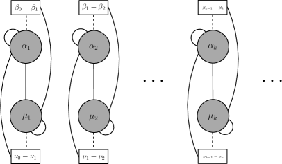
Figure 2: The proposed quantum mechanical quiver. This follows from the analysis of open strings in the Hanany-Witten set-up.

3 Connection with the $\text{AdS}_{2}\times\text{S}^{2}\times\text{CY}_{2}\times\Sigma$ backgrounds of Chiodaroli-Gutperle-Krym

In this section we relate our backgrounds to the general class of $\text{AdS}_{2}\times\text{S}^{2}\times\text{CY}_{2}\times\Sigma$ solutions to Type IIB supergravity with 8 supercharges found by Chiodaroli, Gutperle and Krym (CGK) in [34]. We show that our solutions fit locally in their classification in the absence of D3 and D7 brane sources (in this sense our backgrounds extend those in [34] at the AdS₂ point). A similar analysis shows that the family of $\text{AdS}_{2}$ solutions to Type IIB supergravity recently found in [1] also fits in their general class.

3.1 Review of the CGK geometries

The CGK backgrounds are dual to one dimensional conformal interfaces inside the two dimensional CFT associated to the D1-D5 system. These solutions (unlike ours) interpolate between AdS₂ in the IR (at the interface) and the AdS${}_{3}\times\text{S}^{3}\times\text{CY}_{2}$ solution of Type IIB supergravity in the UV. We shall focus on the AdS₂ fixed points and compare them with both the backgrounds discussed in section 2 and the solutions found in [1].

In [34], the authors used techniques developed in [19, 47] to find half BPS solutions that preserve eight of the sixteen supersymmetries of the AdS${}_{3}\times$S${}^{3}\times$CY₂ vacuum, and are locally asymptotic to this vacuum solution. They provided an ansatz for the bosonic fields in Type IIB supergravity for a foliation of AdS${}_{2}\times$S${}^{2}\times$CY₂ over a two-dimensional Riemann surface $\Sigma$ with a boundary, and found that the local solutions of the BPS equations can be written in terms of two harmonic and two holomorphic functions defined on $\Sigma$. The solutions corresponds to a D1-D5 configuration with extra NS5 branes and fundamental strings, but vanishing D3 and D7 brane charges. We will see that our solutions fit locally within this class of solutions in the absence of D3 and D7 brane sources. Our D3 and D7 sources are localised in $\rho$ and smeared in the $\psi$-coordinate. The mapping explained below is valid at points in $\rho$ where the sources are not present.

We start summarising the local solutions constructed in [34]. The metric for the ten-dimensional spacetime is given, in Einstein frame, by

$$\text{d}s^{2}=f_{1}^{2}\text{d}s_{\text{AdS}_{2}}^{2}+f_{2}^{2}\text{d}s_{\text{S}^{2}}^{2}+f_{3}^{2}\text{d}s_{\text{CY}_{2}}^{2}+\widetilde{\rho}^{2}\text{d}{z}\text{d}{\overline{z}}\,,$$ (3.1)

where the warping factors $f_{i}$ ($i=1,\dots,3$) and $\widetilde{\rho}$ are functions of $z$ and $\overline{z}$, the local holomorphic coordinates of $\Sigma$. The orthonormal frames can be written as,

$$\begin{split}f_{1}^{2}\text{d}s_{\text{AdS}_{2}}^{2}=\eta_{i_{1}i_{2}}e^{i_{1}}\otimes e^{i_{2}}\,,&\quad\quad\quad i_{1,2}=0,1\,,\\ f_{2}^{2}\text{d}s_{\text{S}^{2}}^{2}=\delta_{j_{1}j_{2}}e^{j_{1}}\otimes e^{j_{2}}\,,&\quad\quad\quad j_{1,2}=2,3\,,\\ f_{3}^{2}\text{d}s_{\text{CY}_{2}}^{2}=\delta_{k_{1}k_{2}}e^{k_{1}}\otimes e^{k_{2}}\,,&\quad\quad\quad k_{1,2}=4,5,6,7\,,\\ \widetilde{\rho}^{2}\text{d}{z}\text{d}{\overline{z}}=\delta_{ab}e^{a}\otimes e^{b}\,,&\quad\quad\quad a,b=8,9\,.\end{split}$$ (3.2)

The NS-NS and RR three-forms are written as a complex three-form, defined as $G=e^{\Phi}H_{3}+ie^{-\Phi}(F_{3}-\chi\;H_{3})$. This form is given by,

$$G=g^{(1)}_{a}e^{a01}+g^{(2)}_{a}e^{a23}\,.$$ (3.3)

In turn, the self-dual five-form flux is,

$$F_{5}=h_{a}e^{a0123}+\widetilde{h}_{a}e^{a4567}\,,\quad a=z,\overline{z}\,,$$ (3.4)

where the self-duality condition implies $h_{a}=-\epsilon_{a}\,^{b}\widetilde{h}_{b}$.

The local solutions of the BPS equations and Bianchi identities admit a description in terms of four functions, $A$, $B$, $H$ and $K$. The analysis in [34] shows that the functions $A$ and $B$ must be holomorphic on the Riemann surface $\Sigma$, whilst $H$ and $K$ must be harmonic. The supergravity fields can be written in terms of these functions as,

$$\begin{split}f_{1}^{2}&=\frac{e^{-2\Phi}|H|}{2f_{3}^{2}K}\left((A+\overline{A})K-(B-\overline{B})^{2}\right)\,,\quad\quad f_{2}^{2}=\frac{e^{-2\Phi}|H|}{2f_{3}^{2}K}\left((A+\overline{A})K-(B+\overline{B})^{2}\right)\,,\\ f_{3}^{4}&=4\frac{e^{2\Phi}K}{A+\overline{A}}\,,\quad\quad e^{4\Phi}=\frac{1}{4K^{2}}\left((A+\overline{A})K-(B+\overline{B})^{2}\right)\left((A+\overline{A})K-(B-\overline{B})^{2}\right)\,,\\ \chi&=\frac{1}{2iK}\left(B^{2}-\overline{B}^{2}-(A-\overline{A})K\right)\,,\quad\quad\widetilde{\rho}^{4}=e^{2\Phi}K\frac{(A+\overline{A})}{H^{2}}\frac{|\partial_{z}H|^{4}}{|B|^{4}}\,.\end{split}$$ (3.5)

Here $\Phi=-\phi/2$, where $\phi$ is the dilaton. For the five-form field strength, we define a four-form potential, along CY₂,

$$C_{\text{CY}_{2}}=-\frac{i}{2}\frac{B^{2}-\overline{B}^{2}}{A+\overline{A}}-{2}\widetilde{K},\qquad\qquad\partial_{z}C_{\text{CY}_{2}}=f_{3}^{4}\widetilde{\rho}\;\widetilde{h}_{z}\,,$$ (3.6)

where $\widetilde{K}$ is the harmonic function conjugate to $K$.

The potentials for the field strengths in equation (3.3) are written in terms of the holomorphic and harmonic functions as

$$\begin{split}b^{(1)}=-\frac{H(B+\overline{B})}{(A+\overline{A})K-(B+\overline{B})^{2}}-h_{1},\qquad&h_{1}=\frac{1}{2}\int\frac{\partial_{z}H}{B}+\text{c.c.}\;,\\ b^{(2)}=-i\frac{H(B-\overline{B})}{(A+\overline{A})K-(B-\overline{B})^{2}}+\widetilde{h}_{1},\qquad&\widetilde{h}_{1}=-\frac{i}{2}\int\frac{\partial_{z}H}{B}+\text{c.c.}\;,\\ c^{(1)}=-i\frac{H(A\overline{B}-\overline{A}B)}{(A+\overline{A})K-(B+\overline{B})^{2}}+\widetilde{h}_{2},\qquad&\widetilde{h}_{2}=-\frac{i}{2}\int\frac{A\;\partial_{z}H}{B}+\text{c.c.}\;,\\ c^{(2)}=-\frac{H(A\overline{B}+\overline{A}B)}{(A+\overline{A})K-(B-\overline{B})^{2}}+h_{2},\qquad&h_{2}=\frac{1}{2}\int\frac{A\;\partial_{z}H}{B}+\text{c.c.},\;\end{split}$$ (3.7)

where $\widetilde{h}_{i}$ and $h_{i}$ are harmonic functions conjugate to each other. In the previous expression $b^{(1)}$ and $b^{(2)}$ are the potentials of the NS-NS three-form $H_{3}$ and $c^{(1)}$ and $c^{(2)}$ are the potentials related to the RR three-form $F_{3}$. These read,

$$\begin{split}H_{3}=&\text{d}b^{(1)}\wedge{\mathrm{vol}}_{{\mathrm{AdS}}_{2}}+\text{d}b^{(2)}\wedge{\mathrm{vol}}_{\text{S}^{2}}\\ F_{3}=&\mathrm{d}C_{2}-\chi H_{3}=(\mathrm{d}c^{(1)}-\chi\text{d}b^{(1)})\wedge{\mathrm{vol}}_{{\mathrm{AdS}}_{2}}+(\mathrm{d}c^{(2)}-\chi\text{d}b^{(2)})\wedge{\mathrm{vol}}_{\text{S}^{2}}.\end{split}$$ (3.8)

The existence of sensible regular solutions imposes the following conditions on the functions $A$, $B$, $H$ and $K$,

• The harmonic functions $A+\overline{A},B+\overline{B}$ and $K$ must have common singularities.

• No singular points should appear in the bulk of the Riemann surface $\Sigma$.

• The functions $A+\overline{A},K$ and $H$ cannot have any zero in the bulk of the Riemann surface.

• The holomorphic functions $B$ and $\partial_{z}H$ must have common zeros.

The previous conditions guarantee a non-vanishing and finite everywhere $f_{1}$ (except at isolated singular points at the boundary), a finite $f_{2}$ in the interior of the Riemann surface and vanishing at the boundary, and, finally, finite and non-vanishing $f_{3}$ and $e^{2\Phi}$ functions everywhere on the Riemann surface, including the boundary.

The equations in (3.5) can be inverted to find $A$, $B$, $H$ and $K$ in terms of $f_{i}$ ($i=1,\dots,3$), $\chi$ and $\Phi$. One finds two possibilities, that we will refer as the “plus and minus solutions”,

$$\text{Sol}_{+}:\; H=f_{1}f_{2}f_{3}^{2},\quad K_{+}=\frac{f_{1}f_{3}^{4}}{2f_{2}},\quad A_{+}=\frac{f_{1}}{f_{2}}e^{2\Phi}-i\chi,\quad B_{+}=\frac{e^{\Phi}f_{3}^{2}}{2f_{2}}\sqrt{f_{1}^{2}-f_{2}^{2}}\;,$$ (3.9)

$$\text{Sol}_{-}:\; H=f_{1}f_{2}f_{3}^{2},\quad K_{-}=\frac{f_{2}f_{3}^{4}}{2f_{1}},\quad A_{-}=\frac{f_{2}}{f_{1}}e^{2\Phi}-i\chi,\quad B_{-}=i\;\frac{e^{\Phi}f_{3}^{2}}{2f_{1}}\sqrt{f_{1}^{2}-f_{2}^{2}}.$$ (3.10)

Inserting the “plus-solution”, equation (3.9), or the “minus-solution”, equation (3.10), in the first expression of (3.6) one obtains, in both cases, the function associated to the 4-form potential,

$$C_{\text{CY}_{2}}=-2\widetilde{K},$$ (3.11)

where $\widetilde{K}$ is the harmonic function conjugate to $K$, according the footnote 1.

In the next subsection we obtain the harmonic and holomorphic functions that give rise to our backgrounds in eqs. (2.1)-(2.2), as well as to the geometries in [1].

3.2 Our AdS₂ geometries and the “plus-solution”

In order to compare the generic backgrounds given by eqs.(2.1)-(2.2) with the solutions in [34, 35] we express our solutions in Einstein frame, to agree with their conventions. We obtain,

$$\begin{split}f_{1}^{2}=\frac{u}{\sqrt{2}}\left(\frac{\widehat{h}_{4}h_{8}^{3}}{(4\widehat{h}_{4}h_{8}-(u^{\prime})^{2})^{3}}\right)^{1/4},\qquad f_{2}^{2}=\frac{u}{\sqrt{2^{5}}}\left(\frac{4\widehat{h}_{4}h_{8}-(u^{\prime})^{2}}{\widehat{h}_{4}^{3}h_{8}}\right)^{1/4},\\ f_{3}^{2}=\left(\frac{\widehat{h}_{4}(4\widehat{h}_{4}h_{8}-(u^{\prime})^{2})}{2^{2}h_{8}}\right)^{1/4},\qquad e^{2\Phi}=e^{-\phi}=\frac{1}{2}\sqrt{\frac{h_{8}}{\widehat{h}_{4}}}\sqrt{4\widehat{h}_{4}h_{8}-(u^{\prime})^{2}},\\ \chi=h_{8}^{\prime}\psi,\qquad\widetilde{\rho}^{2}=\frac{1}{\sqrt{2}u}\left(\widehat{h}_{4}h_{8}^{3}(4\widehat{h}_{4}h_{8}-(u^{\prime})^{2})\right)^{1/4},\qquad C_{\text{CY}_{2}}=-h_{4}^{\prime}\psi.\end{split}$$ (3.12)

We emphasise that these expressions are valid at the points where $h_{8}^{\prime\prime}=\widehat{h}_{4}^{\prime\prime}=0$.

We take the $\rho$ and $\psi$ coordinates to define the real and imaginary parts of the $z$ variable. With this parametrisation, $\Sigma$ is an annulus, defined in the complex plane (see Figure 3),

$$z=\psi+i\rho\qquad\text{with}\qquad\psi\in[0,2\pi]\qquad\text{and}\qquad\rho\in[0,2\pi(P+1)]\,.$$ (3.13)

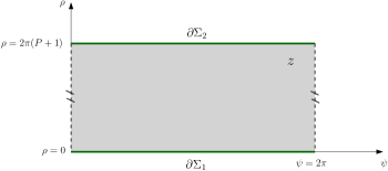
Figure 3: Riemann surface associated to our AdS₂ geometries. Given the periodicity of $\psi$ it defines an annulus.

Locally, our solutions are defined by the three functions $u,\widehat{h}_{4},h_{8}$, which must be linear in $\rho$. We take

$$u=u_{0}+u_{1}\rho,\qquad h_{8}=\mu+\nu\rho,\qquad\widehat{h}_{4}=\alpha+\beta\rho.$$ (3.14)

Substituting (3.12) in (3.9) and taking into account (3.14), we find for the functions $A,B,H,K$,

$$\begin{split}A=&h_{8}-i\psi h_{8}^{\prime}=\mu-i\nu z,\qquad B=\frac{u^{\prime}}{4}=\frac{u_{1}}{4}\,,\\ H=&\frac{u}{4}=\frac{u_{0}}{4}-i\frac{u_{1}}{8}(z-\overline{z})\,,\qquad K=\frac{\widehat{h}_{4}}{2}=\frac{\alpha}{2}-i\frac{\beta}{4}(z-\overline{z})\,.\end{split}$$ (3.15)

It is easy to check that $H$, $K$, $A+\overline{A}$ and $B+\overline{B}$ are harmonic functions and $A$ and $B$ are holomorphic. The harmonic function $\widetilde{K}$ reads, in turn,

$$\widetilde{K}=-\frac{\widehat{h}_{4}^{\prime}}{4}(z+\overline{z})=-\frac{\beta}{{4}}(z+\overline{z})\,,$$ (3.16)

which is the harmonic function conjugate to the expression for $K$ in (3.15).

From the equations (3.7), and using (3.15), we can then obtain the harmonic functions and potentials associated with the NS-NS three-form,

$$\begin{split}&h_{1}=-\frac{i}{4}(z-\overline{z})\,,\qquad\widetilde{h}_{1}=-\frac{1}{4}(z+\overline{z})\,,\\ &b^{(1)}=\frac{u_{1}(2u_{0}-iu_{1}(z-\overline{z}))}{u_{1}^{2}+(2i\alpha+(z-\overline{z})\beta)(2i\mu+(z-\overline{z})\nu)}-h_{1}\,,\qquad b^{(2)}=-\frac{1}{4}(z+\overline{z})\,,\end{split}$$ (3.17)

as well as those associated with the RR three-form,

$$\begin{split}&h_{2}=-\frac{\nu}{8}(z^{2}+\overline{z}^{2})-\frac{i}{4}\mu(z-\overline{z})\,,\qquad\widetilde{h}_{2}=i\frac{\nu}{8}(z^{2}-\overline{z}^{2})-\frac{\mu}{4}(z+\overline{z})\,,\\ &c^{(1)}=\frac{u_{1}(2u_{0}-iu_{1}(z-\overline{z}))(z+\overline{z})\nu}{8(u_{1}^{2}+(2i\alpha+(z-\overline{z})\beta)(2i\mu+(z-\overline{z})\nu))}+\widetilde{h}_{2}\,,\qquad c^{(2)}=-\frac{u_{1}(2iu_{0}+u_{1}(z-\overline{z}))}{8(\beta(z-\overline{z})+2i\alpha)}+h_{2}\,.\end{split}$$ (3.18)

From these expressions we can recover $H_{3}$ and $F_{3}$ as given in eqs. (2.1)-(2.2). Note that $h_{i}$ and $\widetilde{h}_{i}$ are harmonic functions conjugate to each other.

We have thus shown that our solutions can be obtained, locally, from the class of solutions constructed in [34]. Note that in our analysis we have implicitly assumed that $h_{8}^{\prime\prime}=0$ and $\widehat{h}_{4}^{\prime\prime}=0$ also hold globally. This is necessary in order to match the axion and the 4-form RR potential given in (3.12). This assumption –translated to our geometries– indicates that we are not allowing for D7 and D3 brane sources, according to equations (2.22)-(2.23). This agrees with the analysis in [34], which does not include either these types of branes.

We will show in subsection 3.4 that D3-brane sources can be included in the two boundaries of the annulus following the formalism for the annulus derived in [35]. This allows to recover the solutions in our class where D3-branes terminate the space at $\rho=2\pi(P+1)$. Quite surprisingly, we will also see that, even if not included in the analysis in [35], D7-brane sources can also be allowed at the end of the space. We will show that they also manifest as (smeared) singularities of the basic harmonic function defined in the annulus in [35].

Before that, we show in the next subsection that the AdS₂ geometries found in [1], that we will refer as LNRS geometries, fit as well in the CGK class.

3.3 The LNRS geometries and the “minus-solution”

As we already mentioned in section 2, our class of geometries can be obtained through a double analytic continuation from the AdS₂ solutions studied in [1]. In this section we show that the latter fit within the class of solutions referred as “minus solutions” in [34].

The warping factors, dilaton, axion and RR 4-form potential associated to the AdS₂ geometries constructed in [1] (in Einstein frame) are given by,

$$\begin{split}f_{1}^{2}=\frac{u}{\sqrt{2^{5}}}\left(\frac{4\widehat{h}_{4}h_{8}+(u^{\prime})^{2}}{\widehat{h}_{4}^{3}h_{8}}\right)^{1/4}\,,\qquad f_{2}^{2}=\frac{u}{\sqrt{2}}\left(\frac{\widehat{h}_{4}h_{8}^{3}}{(4\widehat{h}_{4}h_{8}+(u^{\prime})^{2})^{3}}\right)^{1/4}\,,\\ f_{3}^{2}=\frac{1}{\sqrt{2}}\left(\frac{\widehat{h}_{4}(4\widehat{h}_{4}h_{8}+(u^{\prime})^{2})}{h_{8}}\right)^{1/4}\,,\qquad e^{2\Phi}=e^{-\phi}=\frac{1}{2}\sqrt{\frac{h_{8}}{\widehat{h}_{4}}}\sqrt{4\widehat{h}_{4}h_{8}+(u^{\prime})^{2}}\,,\\ \chi=h_{8}^{\prime}\psi\,,\qquad\widetilde{\rho}^{2}=\frac{1}{\sqrt{2}u}\left(\widehat{h}_{4}h_{8}^{3}(4\widehat{h}_{4}h_{8}+(u^{\prime})^{2})\right)^{1/4},\qquad C_{\text{CY}_{2}}=-h_{4}^{\prime}\psi\,.\end{split}$$ (3.19)

The Riemann surface is the same one defined in equation (3.13) and Figure 3, and, as in the previous subsection, we are also taking $h_{8}^{\prime\prime}=0$ and $\widehat{h}_{4}^{\prime\prime}=0$ globally, i.e. solutions without D7 and D3 brane sources. This is needed to obtain the axion and RR 4-form potential of the previous equations.

In this case the matching with the solutions in [34] is with the “minus-solutions” defined by equation (3.10). Taking into account (3.14), the harmonic and holomorphic functions read,

$$\begin{split}A=h_{8}-i\psi h_{8}^{\prime}=\mu-i\;\nu z\,,&\qquad B=i\;\frac{u^{\prime}}{4}=i\;\frac{u_{1}}{4}\,,\\ H=\frac{u}{4}=\frac{u_{0}}{4}-i\frac{u_{1}}{8}(z-\overline{z})\,,&\qquad K=\frac{\widehat{h}_{4}}{2}=\frac{\alpha}{2}-i\;\frac{\beta}{4}(z-\overline{z})\,.\end{split}$$ (3.20)

As in the previous subsection, the functions $H$, $K$, $A+\overline{A}$ $B+\overline{B}$ are harmonic and $A$ and $B$ holomorphic. The harmonic function $\widetilde{K}$ reads exactly as in (3.16).

In turn, the harmonic functions that give rise to the NS-NS and RR three-forms read,

$$\begin{split}&h_{1}=-\frac{1}{4}(z+\overline{z}),\qquad\widetilde{h}_{1}=\frac{i}{4}(z-\overline{z}),\\ &h_{2}=-\frac{\mu}{4}(z+\overline{z})+i\frac{\nu}{8}(z^{2}-\overline{z}^{2}),\qquad\widetilde{h}_{2}=i\frac{\mu}{4}(z-\overline{z})+\frac{\nu}{8}(z^{2}+\overline{z}^{2}),\\ &b^{(1)}=\frac{1}{4}(z+\overline{z})\,,\qquad b^{(2)}=\frac{u_{1}(2u_{0}-iu_{1}(z-\overline{z}))}{4(u_{1}^{2}-(2i\mu+\nu(z-\overline{z}))(2i\alpha+\beta(z-\overline{z})))}+\widetilde{h}_{1}\,,\\ &c^{(1)}=-\frac{u_{1}(u_{1}(z-\overline{z})+2iu_{0})}{8(2i\alpha+\beta(z-\overline{z}))}+\widetilde{h}_{2}\,,\qquad c^{(2)}=\frac{\nu u_{1}(2u_{0}-iu_{1}(z-\overline{z}))(z+\overline{z})}{8(u_{1}^{2}-(2i\mu+\nu(z-\overline{z}))(2i\alpha+\beta(z-\overline{z})))}+h_{2}\,.\end{split}$$ (3.21)

From these expressions we recover the NS-NS and RR field strengths, $H_{3}$ and $F_{3}$, of the solutions in [1].

3.4 The annulus

As we have already mentioned, the class of solutions constructed in [34] have vanishing D3 and D7-brane charges. Those solutions have a Riemann surface with a single boundary component. In the follow-up paper [35], the authors constructed solutions in which the Riemann surface $\Sigma$ has an arbitrary number of boundaries and non-vanishing D3 brane charges. The D3-branes occur as poles of a basic harmonic function at the boundaries. In this section we consider the simplest case of a Riemann surface with two disconnected boundary components, namely the annulus. We will then see in subsection 3.5 that we can recover the solutions with D3-brane sources at $\rho=2\pi(P+1)$, the end of the space. Quite surprisingly, we will see that D7-branes seem also allowed at the end of the space.

The annulus is defined as,

$$\Sigma\equiv\left\{w\in C,0\leq\text{Re}(w)\leq 1,0\leq\text{Im}(w)\leq\frac{t}{2}\right\},$$ (3.22)

with $t\in\mathbb{R}^{+}$. The points $w+1$ and $w$ are identified, thus giving the topology of an annulus. Its two boundaries, $\partial\Sigma_{1,2}$, are located at Im$(w)=0$ and Im$(w)=\frac{t}{2}$. The annulus can be constructed from a double surface $\widehat{\Sigma}$, which is defined as a rectangular torus with periods 1 and $\tau$, where $\tau$ is a purely imaginary parameter, $\tau=it$. The original surface $\Sigma$ is obtained as the quotient $\Sigma=\widehat{\Sigma}/\mathcal{J}$ where $\mathcal{J}(z)=\overline{z}$.

The construction of the solutions for the annulus in [35] proceeds in three steps. First, a basic harmonic function with singularities and suitable boundary conditions is constructed. Second, the harmonic functions, $A+\overline{A}$, $H$ and $K$, are expressed as linear superpositions of the basic harmonic function, evaluated at the various poles in the two boundaries. Finally, the meromorphic function $B$ is constructed such that it satisfies certain regularity conditions. Some of these conditions come from imposing that the solutions asymptote locally to the AdS${}_{3}\times\text{S}^{3}\times\text{CY}_{2}$ background. These regularity conditions will not be satisfied by our solutions, first because they do not asymptote to this geometry and, second, because the D3-branes (also the D7-branes) are smeared in the $\psi$ direction. This introduces significant changes in the regularity analysis. For this reason we will not give a detailed account of the regularity conditions imposed in [35]. We will see however in the next subsection that our solutions can still be recovered from the general formalism in [35] in an appropriate limit.

The construction in [35] of the basic harmonic function is carried out in terms of elliptic functions and their related Jacobi theta function of the first kind,

$$\theta_{1}(w|\tau)=2\sum_{n=0}^{\infty}(-1)^{n}e^{i\pi\tau(n+\frac{1}{2})^{2}}\sin[(2n+1)w],$$ (3.23)

as follows,

$$h_{0}(w,\overline{w})=i\left(\frac{\partial_{w}\theta_{1}(\pi w|\tau)}{\theta_{1}(\pi w|\tau)}+\frac{2\pi iw}{\tau}\right)+\text{c.c.}$$ (3.24)

This function has the following simple properties: it has a single simple pole on $\partial\Sigma$, it satisfies Dirichlet conditions away from the pole, and it is positive in the interior of $\Sigma$.

Notice that $h_{0}(w,\overline{w})$ has a singularity at $w=0$, on the first boundary. This pole can be shifted to any point on $\partial\Sigma_{1}$ by a real translation, so that $h_{0}(w-x,\overline{w}-x)$ has a singularity at $w=x$. Instead, to obtain the harmonic functions with singularities at $\partial\Sigma_{2}$ one needs to define,

$$w^{\prime}\equiv\frac{\tau}{2}-w.$$ (3.25)

Then the function $h_{0}(w^{\prime}+y,\overline{w}^{\prime}+y)$ has a pole at $w^{\prime}=-y$, on the second boundary, for a real $y$. In other words the pole is localised at $w=y+it/2$.

In the annulus the harmonic functions $A+\overline{A}$, $B+\overline{B}$, $H$ and $K$ are expressed as linear combinations of $h_{0}$ harmonic functions with poles on both boundaries,

$$\begin{split}A+\overline{A}=&\sum_{\ell_{A}=1}^{M_{A}}r_{\ell_{A}}h_{0}(w-x_{\ell_{A}},\overline{w}-x_{\ell_{A}})+\sum_{j_{A}=1}^{M^{\prime}_{A}}r^{\prime}_{j_{A}}h_{0}(w^{\prime}+y_{j_{A}},\overline{w}^{\prime}+y_{j_{A}}),\\ B+\overline{B}=&\sum_{\ell_{B}=1}^{M_{B}}r_{\ell_{B}}h_{0}(w-x_{\ell_{B}},\overline{w}-x_{\ell_{B}})+\sum_{j_{B}=1}^{M^{\prime}_{B}}r^{\prime}_{j_{B}}h_{0}(w^{\prime}+y_{j_{B}},\overline{w}^{\prime}+y_{j_{B}}),\\ H=&\sum_{\ell_{H}=1}^{M_{H}}r_{\ell_{H}}h_{0}(w-x_{\ell_{H}},\overline{w}-x_{\ell_{H}})+\sum_{j_{H}=1}^{M^{\prime}_{H}}r^{\prime}_{j_{H}}h_{0}(w^{\prime}+y_{j_{H}},\overline{w}^{\prime}+y_{j_{H}}),\\ K=&\sum_{\ell_{K}=1}^{M_{K}}r_{\ell_{K}}h_{0}(w-x_{\ell_{K}},\overline{w}-x_{\ell_{K}})+\sum_{j_{K}=1}^{M^{\prime}_{K}}r^{\prime}_{j_{K}}h_{0}(w^{\prime}+y_{j_{K}},\overline{w}^{\prime}+y_{j_{K}}).\end{split}$$ (3.26)

Each harmonic function is taken to have $M_{i}$ poles $x_{\ell_{i}}$ with $\ell_{i}=1,...,M_{i}$ on $\partial\Sigma_{1}$, and $M_{i}^{\prime}$ poles $y_{j_{i}}$ with $j_{i}=1,...,M^{\prime}_{i}$ on $\partial\Sigma_{2}$. The corresponding residues are $r_{\ell_{i}}$ and $r_{j_{i}}$.

In addition to the regularity conditions given in subsection 3.1, the harmonic functions (3.26) satisfy an extra condition coming from the requirement that $e^{4\Phi}>0$. Namely, $(A+\overline{A})K-(B+\overline{B})^{2}>0$ must be obeyed throughout $\Sigma$. Furthermore, in this language the first regularity condition can be written in terms of the residues as $r_{A}r_{K}=r_{B}^{2}$.

3.5 Zoom-in to our solutions

In this subsection we show that it is possible to recover well-defined global solutions with source branes at the ends of the space from the general analysis above for the annulus. These solutions do not satisfy most of the regularity conditions imposed in [34, 35], and, moreover, contain not only D3 but also D7-brane sources at the ends of the space. Still, we will be able to recover them in a particular limit from the formalism in [35].

As we have already stressed, the choice of constants in the general $\widehat{h}_{4}$ and $h_{8}$ functions defined by equations (2.9) and (2.13) allows for discontinuities in the RR sector of our backgrounds at each $\rho=2\pi k$ value, with $k=1,\dots,P$. The discontinuities in $\widehat{h}_{4}^{\prime}$ are interpreted as generated by D3-brane sources, while the discontinuities in $h_{8}^{\prime}$ are interpreted as generated by D7-branes. Both types of branes are smeared in the $\psi$ direction. The space is terminated in the $\rho$ direction by imposing that $\widehat{h}_{4}=h_{8}=0$ at $\rho=0,2\pi(P+1)$. When $u=$ constant the closure of the space by setting $\widehat{h}_{4}=h_{8}=0$ generates D3 and D7 sources, in the boundary of the space, as explained around eq.(2.16).

Instead, in the general discussion for the annulus in [35] the D3-branes occur as poles of a basic harmonic function at its two boundaries. The basic harmonic function must however be regular in the interior. Therefore, in order to fit in the discussion for the annulus we need continuous $\widehat{h}_{4}^{\prime}$ and $h_{8}^{\prime}$ functions. This is imposed taking

$$\beta_{k}\equiv\beta,\qquad\nu_{k}\equiv\nu,\qquad\text{for}\qquad k=0,1,\dots,P,$$ (3.27)

in (2.9), (2.13), which implies

$$\alpha_{k}=k\,\beta,\qquad\mu_{k}=k\,\nu,\qquad\text{for}\qquad k=0,\dots,P.$$ (3.28)

The solutions are then defined by the functions

$$\widehat{h}_{4}=\frac{\beta}{2\pi}\,\rho,\qquad h_{8}=\frac{\nu}{2\pi}\,\rho$$ (3.29)

at all $\rho$-intervals. Yet, the closure of the space at $\rho=2\pi(P+1)$ requires that $(P+1)\beta$ D3-branes and $(P+1)\nu$ D7-branes are present at the end of the space. Instead of closing the space by introducing sources as we did with the choice of $\widehat{h}_{4}$ and $h_{8}$ functions given by (2.9) and (2.13), these branes will be automatically present at the end of the space in the annulus construction.

Let us now see how these solutions arise from the general formalism in [35]. We take the annulus in (3.22) as defined from,

$$\begin{split}&w=\frac{z}{2\pi}=\widetilde{\psi}+i\widetilde{\rho},\quad&\text{with}\qquad\widetilde{\psi}=\frac{\psi}{2\pi},\quad\widetilde{\rho}=\frac{\rho}{2\pi}.\end{split}$$ (3.30)

Then $\widetilde{\psi}\in[0,1]$ and the parameter $t$ in the definition of the annulus is $t=2(P+1)$. As recalled in section 2, our class of solutions is valid when $P$ is large. This allows us to approximate the Jacobi theta function introduced in (3.23) by its asymptotic expansion when $t\to\infty$,

$$\theta_{1}(\pi w|\tau)|_{t\to\infty}\approx 2e^{-\frac{\pi}{4}t}\sin{\pi w}\approx ie^{-\frac{\pi}{4}t}e^{-i\pi w}.$$ (3.31)

This approximation will be key in showing the matching with our solutions. Indeed, in this approximation it is easy to see that the basic harmonic function defined by (3.24) reads,

$$h_{0}(w,\overline{w})\approx 2\pi+\frac{i\pi}{P+1}(w-\overline{w}).$$ (3.32)

This gives, at the two boundaries $\partial\Sigma_{1}$ and $\partial\Sigma_{2}$,

$$\begin{split}&h_{0}(w-x_{\ell_{i}},\overline{w}-x_{\ell_{i}})\approx 2\pi+\frac{i\pi}{P+1}(w-\overline{w}),\\ &h_{0}(w^{\prime}+y_{j_{i}},\overline{w}^{\prime}+y_{j_{i}})\approx-\frac{i\pi}{P+1}(w-\overline{w}),\end{split}$$ (3.33)

respectively, where for the second boundary we have used the relation (3.25). These expressions are thus independent of the positions of the poles at both boundaries. This is in agreement with the fact that our D3/D7 branes are smeared in the $\psi$-direction. We then get for the harmonic functions in eq.(3.26),

$$\begin{split}A+\overline{A}=&2\pi\sum_{\ell_{A}=1}^{M_{A}}r_{\ell_{A}}-\frac{i\pi}{P+1}(w-\overline{w})\left(\sum_{j_{A}=1}^{M^{\prime}_{A}}r^{\prime}_{j_{A}}-\sum_{\ell_{A}=1}^{M_{A}}r_{\ell_{A}}\right),\\ B+\overline{B}=&2\pi\sum_{\ell_{B}=1}^{M_{B}}r_{\ell_{B}}-\frac{i\pi}{P+1}(w-\overline{w})\left(\sum_{j_{B}=1}^{M^{\prime}_{B}}r^{\prime}_{j_{B}}-\sum_{\ell_{B}=1}^{M_{B}}r_{\ell_{B}}\right),\\ H=&2\pi\sum_{\ell_{H}=1}^{M_{H}}r_{\ell_{H}}-\frac{i\pi}{P+1}(w-\overline{w})\left(\sum_{j_{H}=1}^{M^{\prime}_{H}}r^{\prime}_{j_{H}}-\sum_{\ell_{H}=1}^{M_{H}}r_{\ell_{H}}\right),\\ K=&2\pi\sum_{\ell_{K}=1}^{M_{K}}r_{\ell_{K}}-\frac{i\pi}{P+1}(w-\overline{w})\left(\sum_{j_{K}=1}^{M^{\prime}_{K}}r^{\prime}_{j_{K}}-\sum_{\ell_{K}=1}^{M_{K}}r_{\ell_{K}}\right).\end{split}$$ (3.34)

In order to match these expressions with the expressions for $A+\overline{A}$ and $K$ given in eq.(3.15) we take into account that $w=z/(2\pi)$, and we obtain,

$$\sum_{\ell_{A}=1}^{M_{A}}r_{\ell_{A}}=0\qquad\text{and}\qquad\sum_{j_{A}=1}^{M^{\prime}_{A}}r^{\prime}_{j_{A}}=\frac{(P+1)\nu}{4\pi},$$ (3.35)

for the matching of $A+\overline{A}$, and

$$\sum_{\ell_{K}=1}^{M_{K}}r_{\ell_{K}}=0\qquad\text{and}\qquad\sum_{j_{K}=1}^{M^{\prime}_{K}}r^{\prime}_{j_{K}}=\frac{(P+1)\beta}{\pi},$$ (3.36)

for the matching of $K$. Rescaling the residues as

$$r^{\prime}_{j_{A}}\to 2r^{\prime}_{j_{A}},\qquad r^{\prime}_{j_{K}}\to\frac{r^{\prime}_{j_{K}}}{4}.$$ (3.37)

and replacing the sums by

$$\sum_{j_{A}=1}^{M^{\prime}_{A}}r^{\prime}_{j_{A}}\rightarrow\frac{1}{2\pi}\int_{0}^{2\pi}dr^{\prime}_{j_{A}},$$ (3.38)

as implied by the smearing of the branes in the $\psi$-direction, we can finally interpret the residues as the charge-densities of D7 and D3 brane sources at both boundaries of the annulus. We would like to stress that even if the general formalism in [35] does not account for D7-branes at the boundaries of the annulus, we have associated these to the (smeared) poles of the basic harmonic function for $A+\overline{A}$. The analysis goes in complete parallelism to the analysis of the residues and poles of the $K$ function, associated to the D3-brane sources at both boundaries of the annulus. It is unclear to us the precise reason why this seems to work in the presence of D7-branes.

Finally, from the matching of the $B+\overline{B}$ and $H$ functions we find

$$\sum_{\ell_{B}=1}^{M_{B}}r_{\ell_{B}}=\sum_{j_{B}=1}^{M^{\prime}_{B}}r^{\prime}_{j_{B}}=0\qquad\text{and}\qquad\sum_{\ell_{H}=1}^{M_{H}}r_{\ell_{H}}=\sum_{j_{H}=1}^{M^{\prime}_{H}}r^{\prime}_{j_{H}}=\frac{u_{0}}{8\pi}.$$ (3.39)

These expressions do not seem to have however a direct interpretation in terms of charges of our solutions.

The previous analysis holds true as well for the LNRS backgrounds discussed in [1]. The matching of the $A+\overline{A}$, $H$ and $K$ functions is valid for both solutions, while the harmonic function $B+\overline{B}$ vanishes. Again, there are smeared D3 and D7-branes at the end of the space with the same relations between residues and charges.

4 A new class of AdS${}_{2}\times\text{S}^{2}\times\text{CY}_{2}\times\Sigma$ solutions with $\Sigma$ an infinite strip

In this section we construct a new class of AdS₂ solutions to Type IIB supergravity with 8 supercharges by acting with non-Abelian T-duality (NATD) on the AdS${}_{3}\times$S${}^{2}\times$CY${}_{2}\times$I_ρ solutions obtained in [23]. The non-Abelian T-duality transformation is performed with respect to a freely acting SL$(2,\mathbb{R})$ isometry group of the AdS₃ subspace. This transformation gives rise to a new class of solutions in which the AdS₃ subspace is replaced by AdS₂ times an interval. These solutions fit in the classification of [34] for a Riemann surface with a single boundary, equivalent to an infinite strip.

4.1 NATD of the AdS${}_{3}\times$S${}^{2}\times$CY₂ solutions

The study of NATD as a solution generating technique of supergravity was initiated in [49]. Further works include [50, 51, 52, 53]. In all these examples the dualisation took place with respect to a freely acting SU(2) subgroup of the entire symmetry group of the solutions. Instead, in this section we perform the non-Abelian T-duality transformation with respect to one of the freely acting SL$(2,\mathbb{R})$ isometry groups of the AdS₃ subspace.

In order to perform the dualisation with respect to the SL$(2,\mathbb{R})$ isometry group we follow the derivation in [54]. We take the $sl(2,\mathbb{R})$ generators analytically continuing the $su(2)$ generators, as $t^{a}=\tau_{a}/\sqrt{2}$, with

$$\tau_{1}=\left(\begin{matrix}&0&i\\ &i&0\end{matrix}\;\;\right),\qquad\tau_{2}=\left(\begin{matrix}&0&-i\\ &i&0\end{matrix}\;\;\right),\qquad\tau_{3}=\left(\begin{matrix}&i&0\\ &0&-i\end{matrix}\;\;\right).$$ (4.1)

These generators satisfy,

$${\rm Tr}(t^{a}t^{b})=(-1)^{a}\delta^{ab},\quad\quad\quad[t^{1},t^{2}]=i\sqrt{2}t^{3},\quad[t^{2},t^{3}]=i\sqrt{2}t^{1},\quad[t^{3},t^{1}]=-i\sqrt{2}t^{2}.$$ (4.2)

A group element in the Euler parametrisation is given by,

$$g=e^{\frac{i}{2}\phi\tau_{3}}e^{\frac{i}{2}\theta\tau_{2}}e^{\frac{i}{2}\psi\tau_{3}},\qquad\text{where}\qquad 0\leq\theta\leq\pi,\;\;0\leq\psi<\infty,\;\;0\leq\phi<\infty,$$ (4.3)

from which we write the left invariant one forms, $L^{a}=-i{\rm Tr}(t^{a}g^{-1}\text{d}g)$, in the following fashion,

$$\begin{split}L^{1}=&\sinh{\psi}\text{d}\theta-\cosh{\psi}\sin{\theta}\text{d}\phi\\ L^{2}=&\cosh{\psi}\text{d}\theta-\sinh{\psi}\sin{\theta}\text{d}\phi\\ L^{3}=&-\cos{\theta}\text{d}\phi-\text{d}\psi.\end{split}$$ (4.4)

The backgrounds in [23] support an SL$(2,\mathbb{R})$ isometry such that the metric, the Kalb-Ramond field and the dilaton can be written as,

$$\begin{split}ds^{2}&=\frac{1}{4}g_{\mu\nu}(x)L^{\mu}L^{\nu}+G_{ij}(x)dx^{i}dx^{j},\qquad B_{2}=B_{ij}(x)dx^{i}\wedge dx^{j},\qquad\phi=\phi(x),\end{split}$$ (4.5)

where $x^{i}$ are the coordinates in the internal manifold, for $i,j=1,2,...,7$, and $L^{\mu}$ are the forms given by (4.4). All the coordinate dependence on the SL$(2,\mathbb{R})$ group is contained in these forms. The subsequent details on how to technically compute the NATD transformation have been developed extensively in the literature [49, 53] (see these reference for more details).

The geometries obtained through NATD with respect to a freely acting SL$(2,\mathbb{R})$ group on the AdS₃ of the solutions in [23] are given by,

$$\begin{split}\text{d}{s}_{st}^{2}&=\frac{u\sqrt{\widehat{h}_{4}h_{8}}}{4r^{2}\widehat{h}_{4}h_{8}-u^{2}}r^{2}\text{d}s_{\text{AdS}_{2}}^{2}+\sqrt{\frac{\widehat{h}_{4}}{h_{8}}}\text{d}s^{2}_{\text{CY}_{2}}+\frac{u\sqrt{\widehat{h}_{4}h_{8}}}{4\widehat{h}_{4}h_{8}+u^{\prime 2}}\text{d}s^{2}_{\text{S}^{2}}+\frac{\sqrt{\widehat{h}_{4}h_{8}}}{u}(\text{d}\rho^{2}+\text{dr}^{2}),\\ e^{-2\phi}&=\frac{\left(4r^{2}\widehat{h}_{4}h_{8}-u^{2}\right)\left(4\widehat{h}_{4}h_{8}+u^{\prime 2}\right)}{2^{8}\widehat{h}_{4}^{2}},\\ B_{2}&=-\frac{2r^{3}\widehat{h}_{4}h_{8}}{4r^{2}\widehat{h}_{4}h_{8}-u^{2}}\text{vol}_{\text{AdS}_{2}}-\frac{4\rho\widehat{h}_{4}h_{8}-u^{\prime}(u-\rho u^{\prime})}{2\left(4\widehat{h}_{4}h_{8}+u^{\prime 2}\right)}\text{vol}_{\text{S}^{2}}.\end{split}$$ (4.6)

Additionally, the background is supported by the RR fluxes,

$$\begin{split}F_{1}=&-\frac{rh^{\prime}_{8}}{4}\text{d}r+\frac{1}{2^{4}}\left(4h_{8}+\partial_{\rho}\left[\frac{uu^{\prime}}{\widehat{h}_{4}}\right]\right)\text{d}\rho,\\ F_{3}=&\frac{h_{8}}{8\left(4\widehat{h}_{4}h_{8}+u^{\prime 2}\right)}\left(\frac{\widehat{h}_{4}^{\prime}u^{2}}{\widehat{h}_{4}}\text{d}\rho+rh_{8}\left(4\widehat{h}_{4}+\partial_{\rho}\left[\frac{uu^{\prime}}{h_{8}}\right]\right)\text{d}r\right)\wedge\text{vol}_{\text{S}^{2}}\\ &+\frac{r^{2}h_{8}}{8\left(4r^{2}\widehat{h}_{4}h_{8}-u^{2}\right)}\left(\frac{h_{8}^{\prime}u^{2}}{h_{8}}\text{d}r-r\widehat{h}_{4}\left(4h_{8}+\partial_{\rho}\left[\frac{uu^{\prime}}{\widehat{h}_{4}}\right]\right)\text{d}\rho\right)\wedge\text{vol}_{\text{AdS}_{2}},\\ F_{5}=&\frac{1}{2^{4}}\left(4r\widehat{h}_{4}^{\prime}\text{d}r-\left(4\widehat{h}_{4}+\partial_{\rho}\left[\frac{uu^{\prime}}{h_{8}}\right]\right)\text{d}\rho\right)\wedge\text{vol}_{\text{CY}_{2}}\\ &-\frac{r^{2}u^{2}h_{8}^{2}}{2^{4}\left(4r^{2}\widehat{h}_{4}h_{8}-u^{2}\right)\left(4\widehat{h}_{4}h_{8}+u^{\prime 2}\right)}\left(4r\widehat{h}_{4}^{\prime}\text{d$\rho$}+\left(4\widehat{h}_{4}+\partial_{\rho}\left[\frac{uu^{\prime}}{h_{8}}\right]\right)\text{d$r$}\right)\wedge\text{vol}_{\text{AdS}_{2}}\wedge\text{vol}_{\text{S}^{2}},\\ F_{7}=&-\frac{\widehat{h}_{4}}{8\left(4\widehat{h}_{4}h_{8}+u^{\prime 2}\right)}\left(\frac{h_{8}^{\prime}u^{2}}{h_{8}}\text{d}\rho+r\widehat{h}_{4}\left(4h_{8}+\partial_{\rho}\left[\frac{uu^{\prime}}{\widehat{h}_{4}}\right]\right)\text{d}r\right)\wedge\text{vol}_{\text{S}^{2}}\wedge\text{vol}_{\text{CY}_{2}}\\ &-\frac{r^{2}\widehat{h}_{4}}{8\left(4r^{2}\widehat{h}_{4}h_{8}-u^{2}\right)}\left(\frac{\widehat{h}_{4}^{\prime}u^{2}}{\widehat{h}_{4}}\text{d}r-rh_{8}\left(4\widehat{h}_{4}+\partial_{\rho}\left[\frac{uu^{\prime}}{h_{8}}\right]\right)\text{d}\rho\right)\wedge\text{vol}_{\text{AdS}_{2}}\wedge\text{vol}_{\text{CY}_{2}},\\ F_{9}=&\frac{r^{2}u^{2}\widehat{h}_{4}^{2}}{4\left(4r^{2}\widehat{h}_{4}h_{8}-u^{2}\right)\left(4\widehat{h}_{4}h_{8}+u^{\prime 2}\right)}\left(rh_{8}^{\prime}\text{d}\rho+\frac{1}{4}\left(4h_{8}+\partial_{\rho}\left[\frac{uu^{\prime}}{\widehat{h}_{4}}\right]\right)\text{d}r\right)\wedge\text{vol}_{\text{AdS}_{2}}\wedge\text{vol}_{\text{CY}_{2}}\wedge\text{vol}_{\text{S}^{2}}.\end{split}$$ (4.7)

The previous background is a solution to the Type IIB supergravity EOM whenever $4r^{2}\widehat{h}_{4}h_{8}-u^{2}>0$. Namely we get a well-defined geometry for

$$r>r_{0}=\frac{u}{2\sqrt{\widehat{h}_{4}h_{8}}}.$$ (4.8)

In the next section we show that a subset of the solutions defined by (4.6) and (4.7) fit in the general classification of AdS${}_{2}\times$S${}^{2}\times$CY${}_{2}\times\Sigma$ geometries given in [34] with $\Sigma$ an infinite strip.

4.2 The NATD solution as a CGK geometry

In this section we discuss how the solutions given by (4.6)-(4.7) fit in the class of CGK. Going to Einstein frame we get the warp factors of the metric, dilaton and axion,

$$\begin{split}&f_{1}^{2}=\frac{ur^{2}\sqrt{h_{8}}(4\widehat{h}_{4}h_{8}+u^{\prime 2})^{1/4}}{4(4\widehat{h}_{4}h_{8}r^{2}-u^{2})^{3/4}},\quad f_{2}^{2}=\frac{u\sqrt{h_{8}}(4\widehat{h}_{4}h_{8}r^{2}-u^{2})^{1/4}}{4(4\widehat{h}_{4}h_{8}+u^{\prime 2})^{3/4}},\\ &f_{3}^{2}=\frac{(4\widehat{h}_{4}h_{8}r^{2}-u^{2})^{1/4}(4\widehat{h}_{4}h_{8}+u^{\prime 2})^{1/4}}{4\sqrt{h_{8}}},\quad e^{2\Phi}=e^{-\phi}=\frac{\sqrt{(4\widehat{h}_{4}h_{8}r^{2}-u^{2})(4\widehat{h}_{4}h_{8}+u^{\prime 2})}}{2^{4}\widehat{h}_{4}},\\ &\chi=\frac{1}{2^{4}}\left(2\nu(\rho^{2}-r^{2})+4\mu\rho+\frac{uu^{\prime}}{\widehat{h}_{4}}\right),\quad\widetilde{\rho}^{2}=\frac{\sqrt{h_{8}}(4\widehat{h}_{4}h_{8}r^{2}-u^{2})^{1/4}(4\widehat{h}_{4}h_{8}+u^{\prime 2})^{1/4}}{2^{2}u}.\end{split}$$ (4.9)

In $\chi$, the axion field, we have taken $h_{8}=\mu+\nu\rho$, with $\mu$, $\nu$ constants. This choice corresponds to backgrounds without D7-branes, as those constructed in [34].

The 2d Riemann surface associated to the solutions is the strip depicted in Figure 4, parametrised as,

$$z=\rho+i\;r\qquad\text{where}\qquad\rho\in[0,2\pi(P+1)]\qquad\text{and}\qquad r\in[r_{0},\infty],$$ (4.10)

where the value of $r_{0}$ is determined in eq.(4.8).

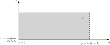
Figure 4: Infinite strip associated to the NATD solution.

Taking the ’plus-solution’ defined by equation (3.9) we obtain the $A$, $B$, $H$ and $K$ functions in terms of the defining functions of our backgrounds, $\widehat{h}_{4}$, $h_{8}$ and $u$,

$$\begin{split}A=\frac{1}{2^{4}}\left(4\mu(r-i\rho)+2i\nu(r-i\rho)^{2}+\frac{u^{\prime}}{\widehat{h}_{4}}(ru^{\prime}-iu)\right),\quad B=\frac{1}{2^{5}}&\frac{\sqrt{4\widehat{h}_{4}h_{8}+u^{\prime 2}}\sqrt{u^{2}+r^{2}u^{\prime 2}}}{\sqrt{\widehat{h}_{4}h_{8}}},\\ H=\frac{ru}{2^{4}},\qquad K=\frac{r(4\widehat{h}_{4}h_{8}+u^{\prime 2})}{2^{5}h_{8}}.\end{split}$$ (4.11)

We anticipate these functions are neither harmonic nor holomorphic. In order to ensure harmonicity -in $H$ and $K$- and holomorphicity -in $A$ and $B$- we need to choose $u^{\prime}=0$. In that case we obtain,

$$\begin{split}&A=\frac{4\mu(r-i\rho)+2i\nu(r-i\rho)^{2}}{2^{4}}=-iz\frac{2\mu+z\nu}{8},\qquad B=\frac{u}{2^{4}}=\frac{u_{0}}{2^{4}},\\ &H=\frac{ru}{2^{4}}=-i\frac{u_{0}}{2^{5}}(z-\overline{z}),\qquad K=\frac{r\widehat{h}_{4}}{2^{3}}=-i\frac{(z-\overline{z})}{2^{5}}(\beta(z+\overline{z})+2\alpha),\end{split}$$ (4.12)

where we have used (3.14). The harmonic function conjugated to $K$ is,

$$\widetilde{K}=-\frac{1}{2^{5}}(\beta(z^{2}+\overline{z}^{2})+2\alpha(z+\overline{z})),\qquad\text{with}\qquad C_{\text{CY}_{2}}=\frac{1}{2^{3}}(\beta(r^{2}-\rho^{2})+2\alpha\rho).$$ (4.13)

Note that we have taken $\widehat{h}_{8}=\alpha+\beta\rho$, with $\alpha$, $\beta$ constants, which corresponds to backgrounds without D3-branes, as those constructed in [34].

The functions associated to the complex three-form are,

$$\begin{split}&h_{1}=-\frac{i}{4}(z-\overline{z}),\qquad\widetilde{h}_{1}=-\frac{1}{4}(z+\overline{z}),\\ &h_{2}=-\frac{1}{2^{5}}\left(\mu(z^{2}+\overline{z}^{2})+\frac{\nu}{3}(z^{3}+\overline{z}^{3})\right),\quad\widetilde{h}_{2}=\frac{i}{2^{5}}\left(\mu(z^{2}-\overline{z}^{2})+\frac{\nu}{3}(z^{3}-\overline{z}^{3})\right).\end{split}$$ (4.14)

Notice that $h_{i}$ and $\widetilde{h}_{i}$ are harmonic functions conjugate to each other. The potentials given in (3.7) are,

$$\begin{split}&b^{(1)}=-i\frac{u_{0}^{2}(z-\overline{z})}{(z-\overline{z})^{2}(\beta(z+\overline{z})+2\alpha)(\nu(z+\overline{z})+2\mu)+4u_{0}^{2}}-h_{1},\qquad b^{(2)}=-\frac{1}{4}(z+\overline{z}),\\ &c^{(1)}=-i\frac{u_{0}^{2}(z-\overline{z})(2\mu(z+\overline{z})+\nu(z^{2}+\overline{z}^{2}))}{16((z-\overline{z})^{2}(\beta(z+\overline{z})+2\alpha)(\nu(z+\overline{z})+2\mu)+4u_{0}^{2})}+\widetilde{h}_{2},\\ &c^{(2)}=-\frac{u_{0}^{2}}{16(\beta(z+\overline{z})+2\alpha)}+h_{2},\end{split}$$ (4.15)

which agree with the expressions (4.6) and (4.7) for $u^{\prime}=0$.

The previous analysis shows that the new class of solutions constructed through non-Abelian T-duality provide an explicit example of CGK geometries where the Riemann surface is an infinite strip. We will provide a more detailed global study of these solutions in a future publication.

5 Electric-magnetic charges and a minimisation principle

In this section we extend two results discussed in [1, 39] to our new infinite family of AdS₂ solutions.
The first result is a relation between the holographic central charge in eq.(2.30) and an integral of the product of the electric and magnetic fluxes of the Dp-branes present in the background. This relates the holographic central charge in Section 2.2, computed purely in terms of the NS-NS sector of the background, with a calculation purely in terms of the Ramond-Ramond sector.
Furthermore, in section 5.2, we explore this relation from a geometrical point of view. We define a quantity in terms of geometric forms in our geometries and through an extremisation principle relate it to the holographic central charge in eq. (2.30). In summary, in this section we present a connection between the holographic central charge, the product of the electric and magnetic charges and an extremised functional.

5.1 A relation between the holographic central charge and the RR fluxes

We provide a relation between the holographic central charge found in eq.(2.30) and the fluxes of the Ramond-Ramond sector in eq (2.2). Consider a Dp brane and the associated electric $\widehat{F}_{p+2}$ and magnetic $\widehat{F}_{8-p}$ Page field strengths. We define the “density of electric and magnetic charges”, $\rho^{e}_{\text{Dp}}$ and $\rho^{m}_{\text{Dp}}$, as follows,

$$\rho_{\text{Dp}}^{e}=\frac{1}{(2\pi)^{p}}\widehat{F}_{p+2},\;\;\;\;\;\rho_{\text{Dp}}^{m}=\frac{1}{(2\pi)^{7-p}}\widehat{F}_{8-p}.$$ (5.1)

From these we construct the quantity,

$$\begin{split}&\int\sum_{p=1,3,5,7}\rho_{\text{D}p}^{e}\rho_{\text{D}p}^{m}=\,\\ &=\frac{1}{\pi}\text{Vol}_{\text{AdS}_{2}}\left(\frac{\text{Vol}_{\text{CY${}_{2}$}}}{16\pi^{4}}\right)\int\text{d}\rho\left[\frac{4\widehat{h}_{4}h_{8}-(u^{\prime})^{2}}{8}+\frac{1}{16}\partial_{\rho}\left(u^{2}\frac{(h_{4}h_{8})^{\prime}}{h_{4}h_{8}}\right)-\frac{u^{2}}{16}\left(\frac{\widehat{h}_{4}^{\prime\prime}}{\widehat{h}_{4}}+\frac{h_{8}^{\prime\prime}}{h_{8}}\right)\right].\end{split}$$ (5.2)

In the absence of sources $\widehat{h}_{4}^{\prime\prime}=h_{8}^{\prime\prime}=0$ and, up to a boundary term, this is proportional to the expression for the holographic central charge in equation (2.30). We explore below the contribution of the sources to this expression. Notice that eq.(LABEL:sumdensities) links the holographic central charge in eq.(2.30)—a calculation purely in terms of the NS-NS sector—with one purely in terms of the Ramond-Ramond sector.

5.2 An action functional for the central charge

Following the ideas of [55, 56] and the lead of the works [1, 39], we construct a functional in terms of an integral of forms defined in the internal space. Once such functional is extremised the holographic central charge in eq.(2.30) is recovered, up to a boundary term.

We define forms $J_{i}$ and ${\mathcal{F}}_{i}$ (for $i=1,3,5,7$) on the internal space $X_{8}=$[S², CY₂, S_ψ, I_ρ]. These forms are inherited from the Page fluxes (2.21). As explained in [1, 39], they are the restriction of the fluxes to the internal space. Writing the Page fluxes in eqs.(2.21) in terms of forms $J_{i}$ and ${\mathcal{F}}_{i}$ as,

$$\begin{split}\widehat{F}_{1}&=J_{1},\qquad\widehat{F}_{3}={\mathcal{F}}_{1}\wedge\text{vol}_{\text{AdS}_{2}}+J_{3},\qquad\widehat{F}_{5}={\mathcal{F}}_{3}\wedge\text{vol}_{\text{AdS}_{2}}+J_{5},\\ \widehat{F}_{7}&={\mathcal{F}}_{5}\wedge\text{vol}_{\text{AdS}_{2}}+J_{7},\qquad\widehat{F}_{9}={\mathcal{F}}_{7}\wedge\text{vol}_{\text{AdS}_{2}}.\end{split}$$ (5.3)

The forms $J_{i}$ and ${\mathcal{F}}_{i}$ are,

$$\begin{split}J_{1}&=h^{\prime}_{8}\,\mathrm{d}\psi\,,\quad\quad J_{3}=\frac{1}{4}\bigg{(}2h_{8}+\frac{u^{\prime}(u\widehat{h}_{4}^{\prime}-\widehat{h}_{4}u^{\prime})}{2\widehat{h}_{4}^{2}}\bigg{)}\text{vol}_{\text{S${}^{2}$}}\wedge\text{d}\rho,\quad\quad J_{5}=-\widehat{h}_{4}^{\prime}\text{vol}_{\text{CY${}_{2}$}}\wedge\mathrm{d}\psi\,\\ J_{7}&=-\frac{1}{4}\left(2\widehat{h}_{4}+\frac{u^{\prime}(uh_{8}^{\prime}-h_{8}u^{\prime})}{2h_{8}^{2}}\right)\text{vol}_{\text{CY${}_{2}$}}\wedge\text{vol}_{\text{S${}^{2}$}}\wedge\text{d}\rho,\;\;\;\;{\mathcal{F}}_{1}=\frac{1}{2}\left(h^{\prime}_{8}(\rho-2\pi k)-h_{8}\right)\text{d}\psi\,,\\ {\mathcal{F}}_{3}&=\frac{1}{4}\left((\rho-2\pi k)h_{8}-\frac{\left(u-(\rho-2\pi k)u^{\prime}\right)(u\widehat{h}_{4}^{\prime}-\widehat{h}_{4}u^{\prime})}{4\widehat{h}_{4}^{2}}\right)\text{vol}_{\text{S${}^{2}$}}\wedge\mathrm{d}\rho,\\ {\mathcal{F}}_{5}&=\frac{1}{2}(\widehat{h}_{4}-(\rho-2\pi k)\widehat{h}_{4}^{\prime})\;\text{vol}_{\text{CY${}_{2}$}}\wedge\mathrm{d}\psi\,,\\ {\mathcal{F}}_{7}&=-\frac{1}{4}\left((\rho-2\pi k)\widehat{h}_{4}-\frac{\left(u-(\rho-2\pi k)u^{\prime}\right)(uh_{8}^{\prime}-h_{8}u^{\prime})}{4h_{8}^{2}}\right)\text{vol}_{\text{CY${}_{2}$}}\wedge\text{vol}_{\text{S${}^{2}$}}\wedge\text{d}\rho.\end{split}$$ (5.4)

With the forms in eqs.(5.4), we construct the functional,

$$\begin{split}{\mathcal{C}}&=\int_{X_{8}}{\mathcal{F}}_{1}\wedge J_{7}+{\mathcal{F}}_{3}\wedge J_{5}-(J_{1}\wedge{\mathcal{F}}_{7}+J_{3}\wedge{\mathcal{F}}_{5})\\ &=\int_{X_{8}}\left(\frac{4\widehat{h}_{4}h_{8}-(u^{\prime})^{2}}{8}-\frac{u^{2}}{16}\left(\frac{\widehat{h}_{4}^{\prime 2}}{\widehat{h}_{4}^{2}}+\frac{h_{8}^{\prime 2}}{h_{8}^{2}}\right)+\frac{uu^{\prime}}{8}\left(\frac{\widehat{h}_{4}^{\prime}}{\widehat{h}_{4}}+\frac{h_{8}^{\prime}}{h_{8}}\right)\right)\text{vol}_{\text{CY}_{2}}\wedge\text{vol}_{\text{S}^{2}}\wedge\text{d}\psi\wedge\text{d}\rho,\end{split}$$ (5.5)

We minimise the functional ${\mathcal{C}}$ by imposing the Euler-Lagrange equation for $u(\rho)$,

$$2u^{\prime\prime}=u\left(\frac{\widehat{h}_{4}^{\prime\prime}}{\widehat{h}_{4}}+\frac{h_{8}^{\prime\prime}}{h_{8}}\right).$$ (5.6)

This equation of motion is solved if,

$$\begin{split}h_{8}^{\prime\prime}=0,\qquad\widehat{h}_{4}^{\prime\prime}=0,\qquad u^{\prime\prime}=0,\end{split}$$ (5.7)

the first two are Bianchi identities for the background and the last is a BPS equation. The functional in eq.(5.5) can be rewritten as,

$$\begin{split}{\mathcal{C}}&=\frac{1}{8}\int_{X_{8}}\left(4\widehat{h}_{4}h_{8}-(u^{\prime})^{2}+\partial_{\rho}\left[\frac{u^{2}}{2}\left(\frac{\widehat{h}_{4}^{\prime}}{\widehat{h}_{4}}+\frac{h_{8}^{\prime}}{h_{8}}\right)\right]-\frac{u^{2}}{2}\left(\frac{\widehat{h}_{4}^{\prime\prime}}{\widehat{h}_{4}}+\frac{h_{8}^{\prime\prime}}{h_{8}}\right)\right)\text{vol}_{\text{CY}_{2}}\wedge\text{vol}_{\text{S}^{2}}\wedge\text{d}\psi\wedge\text{d}\rho.\end{split}$$ (5.8)

The last term (that would vanish in the absence of sources), is proportional to the quotient of the number of flavours by the number of colours in each node. Using the condition that the flavours are sparse, as explained below eq.(2.23), we see that its contribution is subleading in front of the other terms. Furthermore, the boundary term gives a divergent contribution. Indeed, for the case $u=u_{0}$ and $\widehat{h}_{4},h_{8}$ in eqs.(2.9)-(2.13) the boundary term reads,

$$\begin{split}\int_{0}^{2\pi(P+1)}&\partial_{\rho}\left[\frac{u^{2}}{2}\left(\frac{\widehat{h}_{4}^{\prime}}{\widehat{h}_{4}}+\frac{h_{8}^{\prime}}{h_{8}}\right)\right]\text{vol}_{\text{CY}_{2}}\wedge\text{vol}_{\text{S}^{2}}\wedge\text{d}\psi\wedge\text{d}\rho=-\lim_{\epsilon\to 0}\frac{2\pi u_{0}^{2}}{\epsilon}(\alpha_{P}+\mu_{P}+\beta_{0}+\nu_{0})\text{Vol}_{\text{CY}_{2}}\\ &=-\lim_{\epsilon\to 0}\frac{2\pi u_{0}^{2}}{\epsilon}(Q_{\text{D}3}^{total}+Q_{\text{D}7}^{total})\text{Vol}_{\text{CY}_{2}},\end{split}$$ (5.9)

where we regularised $\widehat{h}_{4}(0)=h_{8}(0)=\widehat{h}_{4}(2\pi(P+1))=h_{8}(2\pi(P+1))=\epsilon$. The divergence in eq.(5.9) is associated with the presence of sources in the background as was found in [1, 39].

In summary, the functional in eq.(5.5) is proportional to the holographic central charge of eq.(2.30), plus a subleading contribution and a boundary term. For our infinite family of backgrounds, we have linked a calculation purely in terms of the NS-NS sector—eq.(2.30), with a calculation purely in terms of the Ramond-Ramond sector—eq.(LABEL:sumdensities), with the extremisation of a functional constructed as a restriction of the Ramond-Ramond forms to the internal space—eq.(5.5). We believe that this may be a generic feature, worth exploring in backgrounds dual to various SCFTs in different dimensions.

6 Conclusions

We close this paper by presenting a short summary of the contents of this work and proposing future lines of investigation.

This work presents two new infinite families of backgrounds with an AdS₂ factor. The presentation focuses mostly on geometrical aspects of the new solutions. The new family of backgrounds in Section 2 can be obtained by analytically continuing the backgrounds of [1] or via T-duality, on the Hopf-fibre of the S³, from the solutions in [39]. These connections are summarised in Figure 1. A precise brane set-up was proposed for these backgrounds and the holographic central charge was calculated. We used the brane set-up to argue for a precise quiver. The IR dynamics of such quivers should be the SCQMs dual to our backgrounds.

The family of AdS₂ backgrounds in Section 2 and that in the paper [1] have been shown to be connected to the solutions of [34, 35]. In fact, under certain circumstances they extend this class of solutions. The connection between these qualitatively different backgrounds requires of a subtle zoom-in procedure that we explained in detail in Section 3.

A second family of new backgrounds is presented in Section 4. These interesting solutions depend explicitly on two coordinates (labelled as $\rho$ and $r$ in Section 4) and were obtained by the application of non-Abelian T-duality on the AdS₃ factor of the backgrounds in [23]. We leave for future work to discuss the associated brane set-up, though it seems clear that the ideas described in [40, 41, 42, 43, 14] will play an essential role in the global-definition of these solutions. By the same token, it would be interesting to study the integrability (or not) of the backgrounds presented here, as well as those in [1, 39]. Integrable string backgrounds dual to field theories described by linear quivers in dimensions $d=2,4,6$, have been found in [57, 58, 59, 60]. Similar techniques should probably apply for the $d=1$ case.

Finally, in Section 5 the holographic central charge defined in Section 2—a quantity computed solely in terms of the NS-NS sector of the backgrounds, has been connected with a calculation purely in terms of the Ramond-Ramond sector of our solutions. A functional whose extremisation yields the holographic central charge was also discussed. It should be interesting to find out if a similar structure occurs generically for other AdS_d+1 backgrounds.

References

- [1] Y. Lozano, C. Nunez, A. Ramirez, and S. Speziali, “New AdS2 backgrounds and Conformal Quantum Mechanics,” arXiv:2011.00005 [hep-th].
- [2] J. M. Maldacena, “The Large N limit of superconformal field theories and supergravity,” Int. J. Theor. Phys. 38 (1999) 1113–1133, arXiv:hep-th/9711200 [hep-th]. [Adv. Theor. Math. Phys.2,231(1998)].
- [3] A. Hanany and E. Witten, “Type IIB superstrings, BPS monopoles, and three-dimensional gauge dynamics,” Nucl. Phys. B 492 (1997) 152–190, arXiv:hep-th/9611230.
- [4] F. Apruzzi, M. Fazzi, D. Rosa, and A. Tomasiello, “All AdS7 solutions of type II supergravity,” JHEP 04 (2014) 064, arXiv:1309.2949 [hep-th].
- [5] D. Gaiotto and A. Tomasiello, “Holography for (1,0) theories in six dimensions,” JHEP 12 (2014) 003, arXiv:1404.0711 [hep-th].
- [6] S. Cremonesi and A. Tomasiello, “6d holographic anomaly match as a continuum limit,” JHEP 05 (2016) 031, arXiv:1512.02225 [hep-th].
- [7] C. Nunez, J. M. Penin, D. Roychowdhury, and J. Van Gorsel, “The non-Integrability of Strings in Massive Type IIA and their Holographic duals,” JHEP 06 (2018) 078, arXiv:1802.04269 [hep-th].
- [8] A. Brandhuber and Y. Oz, “The D-4 - D-8 brane system and five-dimensional fixed points,” Phys. Lett. B 460 (1999) 307–312, arXiv:hep-th/9905148.
- [9] O. Bergman and D. Rodriguez-Gomez, “5d quivers and their AdS(6) duals,” JHEP 07 (2012) 171, arXiv:1206.3503 [hep-th].
- [10] Y. Lozano, E. Ó Colgáin, D. Rodriguez-Gómez, and K. Sfetsos, “Supersymmetric via T Duality,” Phys. Rev. Lett. 110 no. 23, (2013) 231601, arXiv:1212.1043 [hep-th].
- [11] E. D’Hoker, M. Gutperle, A. Karch, and C. F. Uhlemann, “Warped in Type IIB supergravity I: Local solutions,” JHEP 08 (2016) 046, arXiv:1606.01254 [hep-th].
- [12] E. D’Hoker, M. Gutperle, and C. F. Uhlemann, “Holographic duals for five-dimensional superconformal quantum field theories,” Phys. Rev. Lett. 118 no. 10, (2017) 101601, arXiv:1611.09411 [hep-th].
- [13] E. D’Hoker, M. Gutperle, and C. F. Uhlemann, “Warped in Type IIB supergravity III: Global solutions with seven-branes,” JHEP 11 (2017) 200, arXiv:1706.00433 [hep-th].
- [14] Y. Lozano, N. T. Macpherson, and J. Montero, “AdS6 T-duals and type IIB AdS S2 geometries with 7-branes,” JHEP 01 (2019) 116, arXiv:1810.08093 [hep-th].
- [15] D. Gaiotto and J. Maldacena, “The Gravity duals of N=2 superconformal field theories,” JHEP 10 (2012) 189, arXiv:0904.4466 [hep-th].
- [16] R. Reid-Edwards and j. Stefanski, B., “On Type IIA geometries dual to N = 2 SCFTs,” Nucl. Phys. B 849 (2011) 549–572, arXiv:1011.0216 [hep-th].
- [17] O. Aharony, L. Berdichevsky, and M. Berkooz, “4d N=2 superconformal linear quivers with type IIA duals,” JHEP 08 (2012) 131, arXiv:1206.5916 [hep-th].
- [18] C. Nunez, D. Roychowdhury, S. Speziali, and S. Zacarias, “Holographic aspects of four dimensional SCFTs and their marginal deformations,” Nucl. Phys. B 943 (2019) 114617, arXiv:1901.02888 [hep-th].
- [19] E. D’Hoker, J. Estes, and M. Gutperle, “Exact half-BPS Type IIB interface solutions. I. Local solution and supersymmetric Janus,” JHEP 06 (2007) 021, arXiv:0705.0022 [hep-th].
- [20] E. D’Hoker, J. Estes, M. Gutperle, and D. Krym, “Exact Half-BPS Flux Solutions in M-theory. I: Local Solutions,” JHEP 08 (2008) 028, arXiv:0806.0605 [hep-th].
- [21] B. Assel, C. Bachas, J. Estes, and J. Gomis, “Holographic Duals of D=3 N=4 Superconformal Field Theories,” JHEP 08 (2011) 087, arXiv:1106.4253 [hep-th].
- [22] C. Couzens, C. Lawrie, D. Martelli, S. Schafer-Nameki, and J.-M. Wong, “F-theory and AdS3/CFT2,” JHEP 08 (2017) 043, arXiv:1705.04679 [hep-th].
- [23] Y. Lozano, N. T. Macpherson, C. Nunez, and A. Ramirez, “AdS3 solutions in Massive IIA with small supersymmetry,” JHEP 01 (2020) 129, arXiv:1908.09851 [hep-th].
- [24] Y. Lozano, N. T. Macpherson, C. Nunez, and A. Ramirez, “1/4 BPS solutions and the AdS3/CFT2 correspondence,” Phys. Rev. D 101 no. 2, (2020) 026014, arXiv:1909.09636 [hep-th].
- [25] Y. Lozano, N. T. Macpherson, C. Nunez, and A. Ramirez, “Two dimensional quivers dual to AdS3 solutions in massive IIA,” JHEP 01 (2020) 140, arXiv:1909.10510 [hep-th].
- [26] Y. Lozano, N. T. Macpherson, C. Nunez, and A. Ramirez, “AdS3 solutions in massive IIA, defect CFTs and T-duality,” JHEP 12 (2019) 013, arXiv:1909.11669 [hep-th].
- [27] Y. Lozano, C. Nunez, A. Ramirez, and S. Speziali, “-strings and AdS3 solutions to M-theory with small supersymmetry,” JHEP 08 (2020) 118, arXiv:2005.06561 [hep-th].
- [28] F. Faedo, Y. Lozano, and N. Petri, “Searching for surface defect CFTs within AdS3,” JHEP 11 (2020) 052, arXiv:2007.16167 [hep-th].
- [29] F. Faedo, Y. Lozano, and N. Petri, “New AdS3 near-horizons in Type IIB,” arXiv:2012.07148 [hep-th].
- [30] G. Dibitetto and N. Petri, “AdS3 from M-branes at conical singularities,” arXiv:2010.12323 [hep-th].
- [31] G. Dibitetto and N. Petri, “AdS2 solutions and their massive IIA origin,” JHEP 05 (2019) 107, arXiv:1811.11572 [hep-th].
- [32] J. P. Gauntlett, N. Kim, and D. Waldram, “Supersymmetric AdS(3), AdS(2) and Bubble Solutions,” JHEP 04 (2007) 005, arXiv:hep-th/0612253.
- [33] N. Kim, “Comments on solutions from M2-branes on complex curves and the backreacted Khler geometry,” Eur. Phys. J. C 74 no. 2, (2014) 2778, arXiv:1311.7372 [hep-th].
- [34] M. Chiodaroli, M. Gutperle, and D. Krym, “Half-BPS Solutions locally asymptotic to AdS(3) x S**3 and interface conformal field theories,” JHEP 02 (2010) 066, arXiv:0910.0466 [hep-th].
- [35] M. Chiodaroli, E. D’Hoker, and M. Gutperle, “Open Worldsheets for Holographic Interfaces,” JHEP 03 (2010) 060, arXiv:0912.4679 [hep-th].
- [36] D. Corbino, E. D’Hoker, J. Kaidi, and C. F. Uhlemann, “Global half-BPS solutions in Type IIB,” JHEP 03 (2019) 039, arXiv:1812.10206 [hep-th].
- [37] D. Corbino, “Warped and symmetry in Type IIB,” arXiv:2004.12613 [hep-th].
- [38] G. Dibitetto, Y. Lozano, N. Petri, and A. Ramirez, “Holographic description of M-branes via AdS2,” JHEP 04 (2020) 037, arXiv:1912.09932 [hep-th].
- [39] Y. Lozano, C. Nunez, A. Ramirez, and S. Speziali, “AdS2 duals to ADHM quivers with Wilson lines,” arXiv:2011.13932 [hep-th].
- [40] Y. Lozano and C. Núñez, “Field theory aspects of non-Abelian T-duality and 2 linear quivers,” JHEP 05 (2016) 107, arXiv:1603.04440 [hep-th].
- [41] Y. Lozano, N. T. Macpherson, J. Montero, and C. Nunez, “Three-dimensional linear quivers and non-Abelian T-duals,” JHEP 11 (2016) 133, arXiv:1609.09061 [hep-th].
- [42] Y. Lozano, C. Nunez, and S. Zacarias, “BMN Vacua, Superstars and Non-Abelian T-duality,” JHEP 09 (2017) 008, arXiv:1703.00417 [hep-th].
- [43] G. Itsios, Y. Lozano, J. Montero, and C. Nunez, “The AdS5 non-Abelian T-dual of Klebanov-Witten as a linear quiver from M5-branes,” JHEP 09 (2017) 038, arXiv:1705.09661 [hep-th].
- [44] N. T. Macpherson, C. Nunez, L. A. Pando Zayas, V. G. J. Rodgers, and C. A. Whiting, “Type IIB supergravity solutions with AdS5 from Abelian and non-Abelian T dualities,” JHEP 02 (2015) 040, arXiv:1410.2650 [hep-th].
- [45] Y. Bea, J. D. Edelstein, G. Itsios, K. S. Kooner, C. Nunez, D. Schofield, and J. A. Sierra-Garcia, “Compactifications of the Klebanov-Witten CFT and new AdS3 backgrounds,” JHEP 05 (2015) 062, arXiv:1503.07527 [hep-th].
- [46] B. Assel and A. Sciarappa, “On monopole bubbling contributions to ’t Hooft loops,” JHEP 05 (2019) 180, arXiv:1903.00376 [hep-th].
- [47] E. D’Hoker, J. Estes, and M. Gutperle, “Gravity duals of half-BPS Wilson loops,” JHEP 06 (2007) 063, arXiv:0705.1004 [hep-th].
- [48] E. D’Hoker, M. Gutperle, and C. F. Uhlemann, “Warped in Type IIB supergravity II: Global solutions and five-brane webs,” JHEP 05 (2017) 131, arXiv:1703.08186 [hep-th].
- [49] K. Sfetsos and D. C. Thompson, “On non-abelian T-dual geometries with Ramond fluxes,” Nucl. Phys. B 846 (2011) 21–42, arXiv:1012.1320 [hep-th].
- [50] Y. Lozano, E. O Colgain, K. Sfetsos, and D. C. Thompson, “Non-abelian T-duality, Ramond Fields and Coset Geometries,” JHEP 06 (2011) 106, arXiv:1104.5196 [hep-th].
- [51] G. Itsios, Y. Lozano, E. O Colgain, and K. Sfetsos, “Non-Abelian T-duality and consistent truncations in type-II supergravity,” JHEP 08 (2012) 132, arXiv:1205.2274 [hep-th].
- [52] G. Itsios, C. Nunez, K. Sfetsos, and D. C. Thompson, “On Non-Abelian T-Duality and new N=1 backgrounds,” Phys. Lett. B 721 (2013) 342–346, arXiv:1212.4840 [hep-th].
- [53] G. Itsios, C. Nunez, K. Sfetsos, and D. C. Thompson, “Non-Abelian T-duality and the AdS/CFT correspondence:new N=1 backgrounds,” Nucl. Phys. B 873 (2013) 1–64, arXiv:1301.6755 [hep-th].
- [54] E. Alvarez, L. Alvarez-Gaume, J. Barbon, and Y. Lozano, “Some global aspects of duality in string theory,” Nucl. Phys. B 415 (1994) 71–100, arXiv:hep-th/9309039.
- [55] C. Couzens, J. P. Gauntlett, D. Martelli, and J. Sparks, “A geometric dual of -extremization,” JHEP 01 (2019) 212, arXiv:1810.11026 [hep-th].
- [56] J. P. Gauntlett, D. Martelli, and J. Sparks, “Toric geometry and the dual of -extremization,” JHEP 01 (2019) 204, arXiv:1812.05597 [hep-th].
- [57] K. Filippas, “Non-integrability on AdS3 supergravity backgrounds,” JHEP 02 (2020) 027, arXiv:1910.12981 [hep-th].
- [58] K. S. Rigatos, “Non-integrability in AdS3 vacua,” arXiv:2011.08224 [hep-th].
- [59] C. Nunez, D. Roychowdhury, and D. C. Thompson, “Integrability and non-integrability in SCFTs and their holographic backgrounds,” JHEP 07 (2018) 044, arXiv:1804.08621 [hep-th].
- [60] K. Filippas, C. Nunez, and J. Van Gorsel, “Integrability and holographic aspects of six-dimensional superconformal field theories,” JHEP 06 (2019) 069, arXiv:1901.08598 [hep-th].