OGLE-2019-BLG-0960Lb: The Smallest Microlensing Planet

Abstract

We report the analysis of OGLE-2019-BLG-0960, which contains the smallest mass-ratio microlensing planet found to date ($q=$1.2–1.6$\times 10^{-5}$ at $1\sigma$). Although there is substantial uncertainty in the satellite parallax measured by Spitzer, the measurement of the annual parallax effect combined with the finite source effect allows us to determine the mass of the host star ($M_{\rm L}=$ 0.3–0.6$\ M_{\odot}$), the mass of its planet ($m_{p}=$1.4–3.1$\ M_{\oplus}$), the projected separation between the host and planet ($a_{\perp}=$ 1.2–2.3 au), and the distance to the lens system ($D_{\rm L}=$ 0.6–1.2 kpc). The lens is plausibly the blend, which could be checked with adaptive optics observations. As the smallest planet clearly below the break in the mass-ratio function (Suzuki et al., 2016; Jung et al., 2019), it demonstrates that current experiments are powerful enough to robustly measure the slope of the mass-ratio function below that break. We find that the cross-section for detecting small planets is maximized for planets with separations just outside of the boundary for resonant caustics and that sensitivity to such planets can be maximized by intensively monitoring events whenever they are magnified by a factor $A>5$. Finally, an empirical investigation demonstrates that most planets showing a degeneracy between $(s>1)$ and ($s<1$) solutions are not in the regime ($|\log s|\gg 0$) for which the “close”/“wide” degeneracy was derived. This investigation suggests a link between the “close”/“wide” and “inner/outer” degeneracies and also that the symmetry in the lens equation goes much deeper than symmetries uncovered for the limiting cases.

1 Introduction

Statistical studies of microlensing planets have shown that while the mass-ratio function for giant planets increases with decreasing mass ratio, $q$, there appears to be a break in the mass-ratio function at small mass ratios. Suzuki et al. (2016) presented the first study to fit a broken power-law to the microlensing planet distribution. They analyzed a sample of 1474 events with 23 planets from the Microlensing Observations in Astrophysics (MOA) survey. Combining their sample with planets from other work (Gould et al., 2010; Cassan et al., 2012), they report a power-law slope for planets with $q<q_{\rm br}$ of $p=0.6$ in contrast to $p=-0.93$ for larger planets (for $dN/d\log q\propto q^{p}$) for a fiducial break at $q_{\rm br}=1.7\times 10^{-4}$. Independently, Udalski et al. (2018) later used a $V/V_{\rm max}$ analysis and a complementary sample to confirm this turnover. Jung et al. (2019) then suggested a much smaller $q_{\rm br}=0.55\times 10^{-4}$ and a change in $p$ above and below the break of $p(q<q_{\rm br})-p(q>q_{\rm br})>3.3$. While this $q_{\rm br}$ is substantially smaller than that of Suzuki et al. (2016), it is consistent within the uncertainty contours of Suzuki et al. (2016) (see their Figure 15). These studies strongly suggest that Neptune/Sun mass-ratio planets are the most common planets at separations of a few au around microlensing host stars.

However, the power-law slope of the mass-ratio distribution below $q_{\rm br}$ and even the exact location of $q_{\rm br}$ are highly uncertain due to a lack of planet detections below this break. In Suzuki et al. (2016), the smallest planet had $q=0.58\times 10^{-4}$, while in Jung et al. (2019), the smallest planet had $q=0.46\times 10^{-4}$. The analysis by Jung et al. (2019) is consistent with a very sharp break at $q_{\rm br}$, i.e., it suggests the possibility that smaller planets might not exist. Hence, depending on the strength of the break, it could be quite difficult to find such planets and so to measure their distribution.

Since that time, three planets have been discovered with mass ratios $q<0.55\times 10^{-4}$, largely due to the Korea Microlensing Telescope Network (KMTNet; Kim et al., 2016). With its $4\ {\rm deg}^{2}$ field of view and telescopes at three sites (CTIO, SAAO, SSO; i.e. KMTC, KMTS, KMTA), KMTNet can achieve near-continuous observations of $92\ {\rm deg}^{2}$ of the bulge at a high cadence. (92, 84, 40, 12 deg²) are covered at cadences of $\Gamma\geq$ (0.2, 0.4, 1, 4) obs hr^-1. This has led to the discovery of KMT-2018-BLG-0029Lb (Gould et al., 2020) and KMT-2019-BLG-0842Lb (Jung et al., 2020) with mass ratios $q=0.18\times 10^{-4}$ and $q=0.41\times 10^{-4}$, respectively. A third planet, in OGLE-2019-BLG-0960, is reported in this work and was discovered through a combination of KMTNet observations and followup data.

While the KMTNet data were crucial to the discovery of the planet in OGLE-2019-BLG-0960, the initial discovery of the event by the Optical Gravitational Lens Experiment (OGLE) was critical for identifying this event as a potential Spitzer target. The early OGLE alert triggered reduction of KMTNet real-time data almost three weeks before the event was discovered by KMTNet. As a result, OGLE-2019-BLG-0960 was under consideration as a potential Spitzer target prior to its discovery by KMTNet. Later, the event was identified as high-magnification, which triggered additional followup observations.

A detailed timeline of the observations is given in Section 2. The analysis of the light curve including the parallax is described in Sections 3 and 4. We derive the properties of the source and the physical parameters of the lens including the planet in Section 5. Then, in Section 6, we consider whether or not the planet was detectable in survey data alone (Section 6.1), and we consider how the sample of small planets can be increased to enable a precise measurement of $q_{\rm br}$ and $p$ for planets with $q<q_{\rm br}$ (Section 6.2). We also explore events with both $(s>1)$ and $(s<1)$ solutions and the relationship to the “close”/“wide” degeneracy of Griest & Safizadeh (1998) (Section 6.3). We conclude in Section 7.

2 Observations

2.1 Ground-Based Survey Observations

OGLE-2019-BLG-0960 was alerted by the OGLE-IV Early Warning System (Udalski, 2003; Udalski et al., 2015) on 23 June 2019 at UT 21:04 (HJD${}^{\prime}=$HJD$-2,450,000=8658.38$). Its coordinates were ${\rm R.A.}=$ 18:16:03.43, ${\rm Decl.}=$ -25:46:28.8 corresponding to $(\ell,b)=(6.10,-4.30)$. It is in OGLE-IV field BLG522, which was observed in the $I$ band with a cadence of $\Gamma\sim 2\,{\rm night}^{-1}$. This event was independently discovered as KMT-2019-BLG-1591 by KMTNet (Kim et al., 2018) on 11 Jul 2019 at UT 03:05 (HJD${}^{\prime}=8675.63$) and as MOA-2019-BLG-324 by Microlensing Observations in Astrophysics (MOA; Bond et al., 2001) on 17 July 2019 at UT 16:07 (HJD${}^{\prime}=8682.17$). This field is observed by KMTNet at a cadence of $\Gamma\sim 0.4\,{\rm hr}^{-1}$. Most of the KMTNet observations were taken in the $I$ band with about 10 in the $V$ band for the purpose of measuring colors. MOA observed the field containing OGLE-2019-BLG-0960  using a custom $R$ filter (which covers standard $R$ and $I$ bands) at a nominal cadence of $\Gamma\sim 0.6\ {\rm hr}^{-1}$, but see below (Section 2.3).

2.2 Spitzer  Observations

OGLE-2019-BLG-0960 was selected for Spitzer  observations and announced as a Spitzer  target on HJD${}^{\prime}=8676.23$ with the condition that it must reach $I<17.45$ prior to HJD${}^{\prime}=8679.5$, i.e., the decision point for the next Spitzer  target upload. Thus, it was initially selected as a “subjective, conditional” target, and observations began at HJD${}^{\prime}=8685.21$. The following week HJD${}^{\prime}\sim 8687$, the event met the “objective” criteria for selecting Spitzer  targets. Thus, observations taken after HJD${}^{\prime}=8691.5$ may be considered “objective”. See Yee et al. (2015) for a detailed explanation of different types of selection and their implications and criteria.

2.3 Ground-Based Followup Observations

Once OGLE-2019-BLG-0960  was selected for Spitzer  observations, we began to monitor it with the dual-channel imager, ANDICAM (DePoy et al., 2003) on the SMARTS 1.3m telescope at CTIO in Chile (CT13). Observations were taken simultaneously in both the $I$ and $H$ bands for the purpose of tracking its evolution and obtaining an $I-H$ color for the source. Starting at HJD${}^{\prime}\sim 8683.5$, we increased the cadence to a few points per night to supplement the survey data in the hopes of better characterizing any planetary perturbations. We also began monitoring the event with the telescopes in the LCO 1-m network at SAAO (South Africa; LCOS) and SSO (Australia; LCOA01, LCOA02).

On 20 Jul 2019, the Spitzer team realized that the event was consistent with high magnification ($A>100$) and sent an alert to the Microlensing Follow-Up Network (MicroFUN) at UT 13:06 (HJD${}^{\prime}=8685.05$) encouraging dense followup observations to capture the peak of the event. Auckland, Farm Cove, and Kumeu Observatories in New Zealand (AO, FCO, and Kumeu, respectively) all responded to the alert and began intensive observations of the event. MOA also increased its cadence in response to the alert. At the same time, we scheduled dense observations with CT13 and the LCO 1-m telescopes at SAAO and SSO. Two days later at HJD${}^{\prime}=8687.05$, we called off the alert because the event was declining and no significant perturbations had been observed over the peak. At this point, most followup observations ceased. However, we continued to observe this event at a cadence of a few per night with CT13, while Kumeu Observatory took an additional hour of normalizing data, which would prove crucial for recognizing and characterizing the planetary perturbation.

On 23 July 2019 (HJD${}^{\prime}=8688.06$), a routine inspection of the CT13 data led to the discovery of a $\sim 0.5$ mag outlier in the light curve. The outlier was confirmed by a data point in the KMTC light curve taken nearly simultaneously. This triggered additional dense observations with the LCO network. We did not realize the existence of Kumeu observations that characterized the falling side of the perturbation until HJD${}^{\prime}\sim 8689.05$.

2.4 Data Reduction and Error Renormalization

The data were reduced by each collaboration and the photometric error bars were renormalized according to the prescription in Yee et al. (2012). Table 1 gives the specific reduction method, the error renormalization factors, and other properties for each data set. In the case of KMTNet data from CTIO and SAAO, we restricted the data to points taken after HJD${}^{\prime}=8616$ to control for possible effects of systematics on the parallax measurement. Likewise, data from KMTA were restricted to $\pm 5$ days from the peak of the event.

3 Ground-Based Light-Curve Analysis

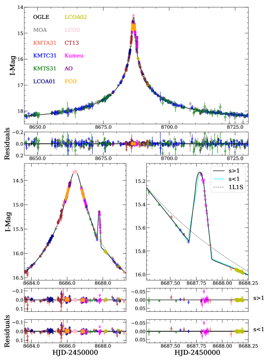
Figure 1: Light curve of OGLE-2019-BLG-0960 with best-fit models. Although the primary evidence for the planet is a strong bump in the light curve at HJD${}^{\prime}\sim 8687.8$, the points before and after the bump also show a negative deviation relative to the best-fit point lens model (dashed gray line), which contributes to the detection. Note that KMTC and CT13 each have a datapoint at HJD${}^{\prime}=8687.796$, but because they are contemporaneous, they do not appear as distinct points on the plot. The two best-fit planetary models are shown as the solid black and cyan lines. Although one model has $s>1$ and one has $s<1$, this degeneracy is far from the regime of the “close”/“wide” degeneracy identified by Griest & Safizadeh (1998, see Section 6.3).

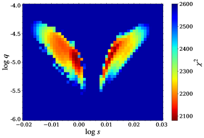
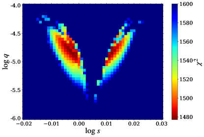
Figure 2: Results of the $s$-$q$ grid-search for the best-fit solutions to the light curve of OGLE-2019-BLG-0960. Left: the fits including all ground-based data yield two distinct minima, one with $s<1$ and one with $s>1$, but not centered around $s=1$. Right: the fits to just the ground-based survey data (OGLE, MOA, KMT) give an additional pair of minima because the caustic crossing is less well-characterized (see Section 6.1).

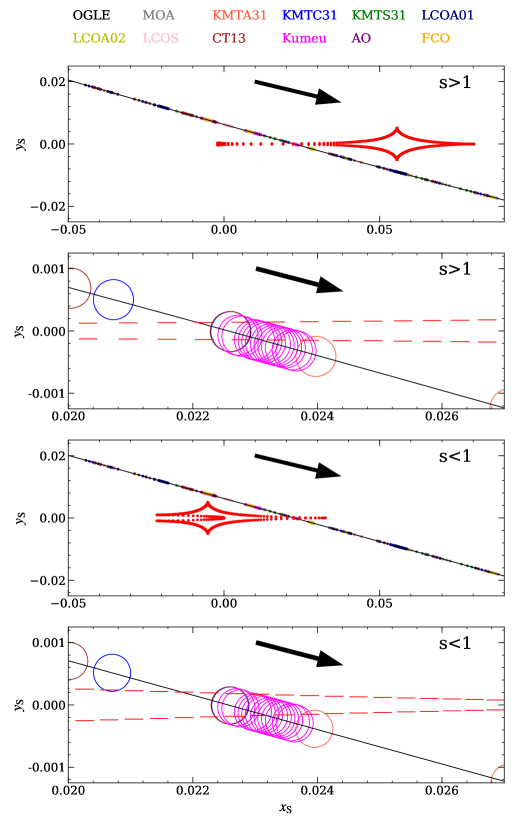
Figure 3: Caustics (red dashed lines) and source trajectory (solid black line and arrow) for the two degenerate solutions for OGLE-2019-BLG-0960. The top two panels show the “$s>1$” solution, and the bottom two panels show the “$s<1$” solution. The top panel in each pair shows the full view of the caustic, while the bottom panel in the pair shows a close up of the caustic crossing. The locations of the source at the times of the observations are indicated by the dots/circles; the size of each circle is set by $\rho$.

The full light curve of this event is shown in Figure 1. With the exception of a brief, 0.2 day, bump that occurs 1.4 days after the peak, the light curve is well described by a standard single-lens single-source (1L1S) Paczynski (1986) fit, which is specified by three geometric parameters, the lens-source closest approach $t_{0}$, the impact parameter $u_{0}$ (normalized to the Einstein radius, $\theta_{\rm E}$), and the Einstein radius crossing time $t_{\rm E}$. In principle, the bump could be explained by either an additional lens (2L1S) or additional source (1L2S), but we begin by focusing on the former. This requires three additional parameters: the companion-host separation $s$ (normalized to $\theta_{\rm E}$), the companion-host mass ratio $q$, and the companion-host orientation $\alpha$ (relative to the direction lens-source relative motion). Because the source transits (or comes very close to) a caustic structure generated by the lens system, we must also specify $\rho\equiv\theta_{*}/\theta_{\rm E}$, where $\theta_{*}$ is the angular radius of the source.

3.1 Static Analysis

We search for the best-fit models following the method of Yang et al. (2020). In brief, we initially conduct a grid search over ($\log s,\log q$) to locate the solutions. For each set of ($\log s,\log q$), we fix $\log s,\log q$, and free $t_{0},u_{0},t_{\rm E},\alpha$ and $\rho$. For the initial values of $t_{0}$, $u_{0}$, and $t_{\rm E}$, we use the values from 1L1S fitting to the light curve excluding the planetary anomaly. The initial values of $\alpha$ and $\rho$ are estimated from the 1L1S parameters as follows:

$$\alpha=\tan^{-1}\frac{t_{\rm eff}}{t_{0,{\rm anom}}-t_{0}}=0.266~{}(15.2^{\circ});\qquad t_{\rm eff}=u_{0}t_{\rm E}$$ (1)

where $t_{0,{\rm anom}}=8687.78$. Using the method of Street et al. (2016), $\rho$ can be estimated by

$$\rho\sim\frac{t_{0,{\rm anom}}-t_{\rm cc}}{t_{\rm E}}\times\sin{\alpha}=3.2\times 10^{-4},$$ (2)

where $t_{\rm cc}\sim 8687.70$ is the time of caustic entry. Then, we search for the best-fit parameters using Markov chain Monte Carlo (MCMC) $\chi^{2}$ minimization as implemented in the emcee ensemble sampler (Foreman-Mackey et al., 2013). We use the advanced contour integration code VBBinaryLensing (Bozza, 2010) to compute the binary-lens magnification. This code uses multiple rings to account for the limb-darkening effect and sets the number of rings automatically based on the required light curve precision. We use linear limb-darkening coefficients for a $T_{\rm eff}=5250$K star: $\Gamma_{I}=0.43$, $\Gamma_{R}=0.52$, $\Gamma_{L}=0.15$ (Claret & Bloemen, 2011).

This grid search yields only two local minima (left panel of Figure 2). We then further refine these minima by allowing all seven parameters to vary in an MCMC. The results are shown in Table 2, and the caustics and source trajectories are shown in Figure 3. As with many events, the two solutions appear to be related by the famous $s\leftrightarrow s^{-1}$ (a.k.a. “close”/“wide”) degeneracy (Griest & Safizadeh, 1998; Dominik, 1999) because one solution has $s<1$ and the other $s>1$. In fact, this is not the case, as we discuss in Section 6.3.

Regardless, the two solutions are very similar in their physical implications. First, the mass ratio is $q=1.27\pm 0.07$ or $q=1.45\pm 0.15\times 10^{-5}$, making this the smallest mass-ratio planet discovered by microlensing to date. Second, although the two solutions are distinct, $s$ is very close to 1, so the separation of the planet from the host star is similar in the two cases. Third, the relatively long Einstein timescale, $t_{\rm E}\sim 62\,$days, suggests that it may be possible to measure the annual parallax effect for this event.

3.2 Ground-based Parallax Analysis

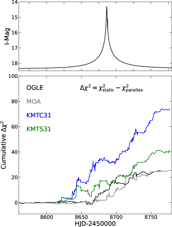
Figure 4: Cumulative distribution of $\Delta\chi^{2}$ as a function of time between the best-fit parallax and static models. For clarity, we only show the $\Delta\chi^{2}$ contributions from the survey data (and we exclude KMTA because only the data over the peak and anomaly are used in the modeling). The top panel shows the model light curve for reference.

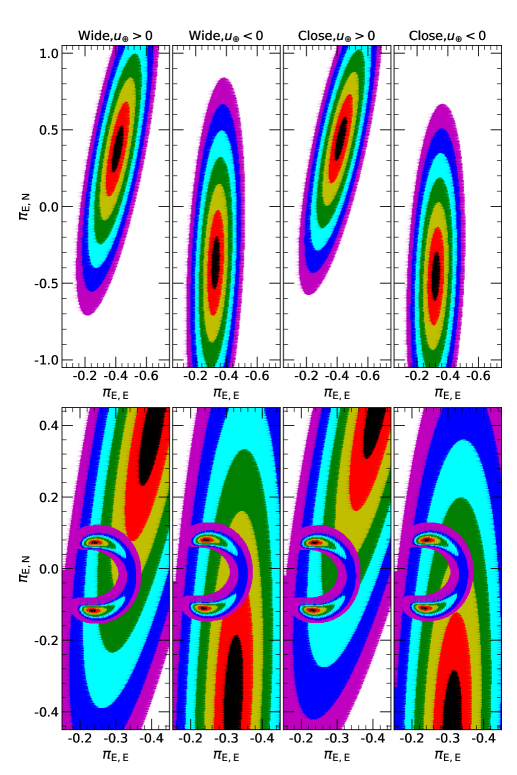
Figure 5: (1, 2, 3, 4, 5, 6, 7)$\sigma$ contours (black, red, yellow, green, cyan, blue, purple) for the parallax vector. The large ellipses in the top panels show the measurement from the annual parallax effect in the ground-based data. These data give a strong constraint on $\pi_{\rm E,\parallel}$, the component of the parallax parallel to the projected position of the Sun, but a relatively weak constraint on $\pi_{\rm E,\perp}$, resulting in highly elliptical error contours. The arcs in the bottom panels are the constraint from the Spitzer-“only” parallax analysis and are overlaid on the annual parallax contours. These show tension with the annual parallax measurement at the $\sim 3\sigma$ level; limits from the blended light are also in tension with the Spitzer-“only” parallaxes. Together, these suggest systematics in the Spitzer light curve may be affecting the parallax measurement.

Thus, we are immediately led to introduce two additional parameters ${\mbox{\boldmath$\pi$}}_{\rm E}=(\pi_{{\rm E},N},\pi_{{\rm E},E})$, i.e., the north and east components of the parallax vector (Gould, 2004) in equatorial coordinates. Because the effect of Earth’s motion can be partially mimicked by lens orbital motion (Batista et al., 2011; Skowron et al., 2011), we initially introduce two further additional parameters ${\mbox{\boldmath$\gamma$}}=((ds/dt)/s,d\alpha/dt)$, i.e., the instantaneous angular velocity at $t_{0}$. We find that $\gamma$ is poorly constrained, so we impose a limit on the ratio of projected kinetic to potential energy (Dong et al., 2009)

$$\beta=\bigg{|}{\frac{\rm KE_{\perp}}{\rm PE_{\perp}}}\bigg{|}={\frac{\kappa M_{\odot}{\rm yr}^{2}}{8\,\pi^{2}}}{\frac{\pi_{\rm E}}{\theta_{\rm E}}}\gamma^{2}\biggl{(}{\frac{s}{\pi_{\rm E}+\pi_{s}/\theta_{\rm E}}}\biggr{)}^{3},$$ (3)

where $\pi_{s}$ is the source parallax. We only accept links on the chain for which $\beta<0.8$. We find that $\gamma$ is neither significantly constrained in the fit nor significantly correlated with ${\mbox{\boldmath$\pi$}}_{\rm E}$, so we suppress these two degrees of freedom.

The final parallax solutions are summarized in Table 2. Figure 4 shows the cumulative $\Delta\chi^{2}$ diagram between the best-fit parallax and static solutions. All of the survey datasets that span the event (OGLE, MOA, KMTC, KMTS) contribute positively and consistently to the parallax signal. This meets our expectation that a real parallax signal should affect data from all observatories and makes it extremely unlikely that the signal has a non-astrophysical origin.

We show in Figure 5 the $\chi^{2}$ contours projected on the ${\mbox{\boldmath$\pi$}}_{\rm E}$ plane, which are in the form of an ellipse with a large axis ratio $a/b\sim 8$ . Such “1-D parallax” measurements were predicted by Gould et al. (1994) and explored in greater detail by Smith et al. (2003) and Gould (2004) for moderately long microlensing events. They arise because $\pi_{{\rm E},\parallel}$, the component of ${\mbox{\boldmath$\pi$}}_{\rm E}$ that is parallel to the projected position the Sun at $t_{0}$, is directly constrained by the asymmetry in the light curve that is induced by Earth’s instantaneous acceleration near the peak of the event. The first clear example of this in a planetary event was OGLE-2005-BLG-071 (Udalski et al., 2005; Dong et al., 2009). Indeed, the orientations (north through east) of the short axes of the ellipses for OGLE-2019-BLG-0960  are close to the projected position of the Sun. Hence, $\pi_{{\rm E},\parallel}$ is both relatively large and well-constrained from the ground-based photometry even though there are substantial uncertainties in the total value of $\pi_{{\rm E}}$.

3.3 Binary Source Models

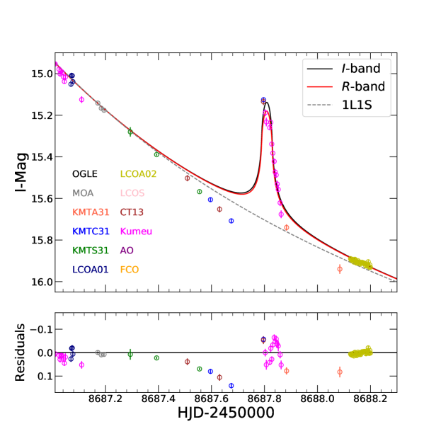
Figure 6: OGLE-2019-BLG-0960 cannot be explained by a point-lens, binary-source (1L2S) model, which is shown in two different bands ($R$, red line, corresponding to the Kumeu Observatory data; $I$, black line, corresponding to CT13 and KMT data). The dotted gray line shows the best-fit point-source/point-lens model.

In principle, a short duration bump on an otherwise point-lens–like light curve can also be caused by a binary source with a large flux ratio (Gaudi, 1998). Hence, we also search for 1L2S solutions. For this search, we introduce the additional parameters $t_{0,2}$ and $u_{0,2}$ to describe the trajectory of the second source and $\rho_{2}$ for its radius. We also introduce $q_{\rm F,I}$, the flux ratio between the two sources, as a fit parameter. The results of these fits are given in Table 3 and show that such solutions are disfavored by $\Delta\chi^{2}>1000$. Figure 6 shows that the best-fit 1L2S model fails to reproduce the decrease in magnification (relative to a point lens) seen before and after the bump.

4 Spitzer Parallax Analysis

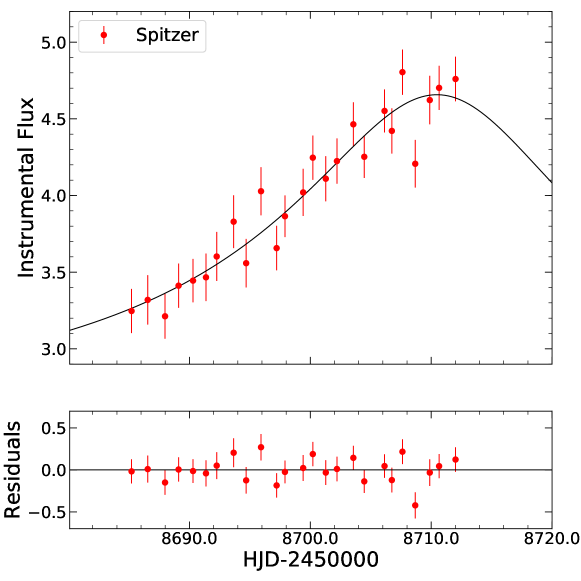
Figure 7: Spitzer light curve (red points) in instrumental-flux units, together with the best-fit Spitzer-“only” model in black. The fact that the event is clearly faint from Spitzer indicates a significant parallax effect. A rising light curve is also consistent with the annual parallax measurement. That is, $\pi_{{\rm E},E}<0$ implies that the event peaked later as seen from Spitzer, which lay to the west of Earth.

According to the original conception of Refsdal (1966), the microlens parallax (${\mbox{\boldmath$\pi$}}_{\rm E}$ in modern notation) could be determined up to a four-fold degeneracy by combining information from the ground-based and space-based Paczyński parameters $(t_{0},u_{0},t_{\rm E})$ for the event,

$${\mbox{\boldmath$\pi$}}_{\rm E}={\frac{{\rm AU}}{D_{\perp}}}\biggl{(}{t_{0,\rm sat}-t_{0,\oplus}\over t_{\rm E}},u_{0,\rm sat}-u_{0,\oplus}\biggr{)},$$ (4)

where ${\bf D_{\perp}}$ is the Earth-satellite separation projected on the plane of the sky and $t_{\rm E}$ is approximated as being the same for both Earth and the satellite. The two terms in Equation (4) are then the components of ${\mbox{\boldmath$\pi$}}_{\rm E}$ that are, respectively, parallel and perpendicular to ${\bf D_{\perp}}$. A four-fold degeneracy arises because $u_{0}$ is a signed quantity, but generally only its magnitude can be determined from the light curve. See Figure 1 of Gould (1994).

Figure 7 shows the Spitzer light curve in instrumental-flux units. Because the Spitzer observations cover the peak of the event (which was very bright, $I=14.3$), the lack of a strong microlensing signal (i.e., a substantial change in the flux) indicates a significant parallax effect. In fact, the Spitzer light curve is rising throughout the observations, which begin approximately at $t_{0,\oplus}$. Because Spitzer was almost due west of Earth at these times, this rising light curve implies that $\pi_{{\rm E},E}<0$, in good agreement with the ground-based results.

However, the total Spitzer flux variation of OGLE-2019-BLG-0960 is extremely small (only 1.5 flux units). Recent experience with KMT-2018-BLG-0029 (Gould et al., 2020), OGLE-2017-BLG-0406 (Hirao et al., 2020), and OGLE-2018-BLG-0799 (Zang et al., 2020) has shown that there can be systematics in the Spitzer parallax measurements for Spitzer light curves with weak signals. Hence, while the Spitzer light curve for OGLE-2019-BLG-0960 shows a clear parallax signal, we must be cautious in interpreting it.

We carry out a quantitative investigation of the Spitzer parallax signal following the method described in Gould et al. (2020). Spitzer-“only” light curves are obtained by fitting only the Spitzer data, while fixing the non-parallax ground-based parameters $(t_{0},u_{0},t_{\rm E},s,q,\alpha,\rho)$ at their best-fit, ground-based values. In particular, because Spitzer-“only” fits are used primarily to analyze information flow rather than to obtain final results, it is best to keep them as simple as possible without tracking finer details. In addition, one must specify the Spitzer source flux (and error bar), both of which can be derived from a Spitzer-ground color-color (e.g., $IHL$) relation together with the $I$-band source flux.

For this color-constraint, we cross-match stars from the $6^{\prime}\times 6^{\prime}$ CT13 $I$-band field with VVV (Minniti et al., 2017) to construct an $I-H$ CMD. While the VVV $H$-band is calibrated, CT13 is not, so the resulting colors are instrumental rather than absolute. In this system, we find the source color is $I_{\rm CT13}-H_{\rm VVV}=3.433\pm 0.013$ (see Section 5.1). When cross-matched to stars in the Spitzer field, this yields a color-color relation:

$$I_{\rm CT13}-L=2.681\pm 0.019.$$ (5)

The resulting parallax contours are shown in Figure 5. This figure shows that the ground-only and Spitzer-“only” contours are inconsistent at the $\sim 3\sigma$ level. Furthermore, we will show in Section 5.4 that the best-fit value for the Spitzer-“only” parallax, $\pi_{\rm E}=0.25$, is in tension with constraints on the lens due to the blended light (unless the host is a stellar remnant).

Because of these tensions, for the remainder of the paper, we focus on what can be derived from the ground-based data alone. In the future, we will carry out a systematic study of low-amplitude Spitzer light curves. Once the impact of systematics on the Spitzer parallax measurements is better understood, we can reassess the constraints from the Spitzer data on this event and assess whether or not it can be included in the Spitzer statistical sample of planets. Ultimately, these tensions can be resolved by separately resolving the source and the lens (assuming that the lens is luminous). This would allow both a measurement of the lens flux and a measurement of the direction of the lens-source relative proper motion (e.g., Batista et al., 2015; Bennett et al., 2015; Bhattacharya et al., 2020; Vandorou et al., 2020). This would both independently constrain the mass of the lens and the direction of the parallax vector (because $\hat{\pi}_{\rm E}\equiv\hat{\mu}_{\rm rel}$).

5 Physical Properties

5.1 CMD & Source Properties

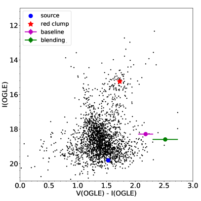
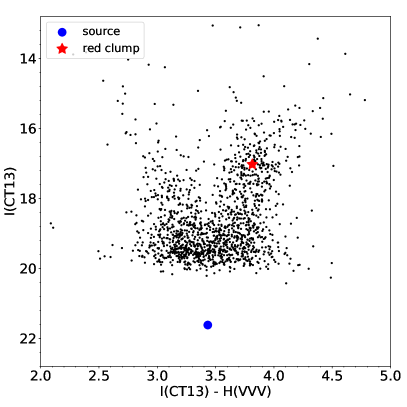
Figure 8: Left: OGLE CMD (calibrated to OGLE-III) of a $120^{\prime\prime}$ square centered on OGLE-2019-BLG-0960. Right: CT13-VVV CMD of a $240^{\prime\prime}$ square centered on the event. In each panel, the red asterisk and blue dot show the centroid of the red clump and the position of the microlens source, respectively. In the left plot, the green and magenta dots show the positions of the blend and the baseline object, respectively. The cyan lines show a naive estimate (see Section 5.4) for the lens color and magnitude calculated for $\theta_{\rm E}\pm 1\sigma$ (solid and dashed lines, respectively); the cyan dot shows the position for $M_{\rm L}=0.5\ M_{\odot}$.

We measure the intrinsic color and magnitude of the source by finding its location in a color-magnitude diagram (CMD) relative to the red clump (Yoo et al., 2004). We do this in two ways. First, we use the OGLE-IV photometry to find $(V-I,I)_{\rm S}=(1.53,19.81)\pm(0.04,0.03)$, and we find the centroid of the red clump is $(V-I,I)_{\rm cl}=(1.73,15.24)\pm(0.02,0.04)$ (see Figure 8). The intrinsic color and magnitude of the red clump along this line of sight is $(V-I,I)_{0,\rm cl}=(1.06,14.27)$ (Bensby et al., 2011; Nataf et al., 2013). This implies that $A_{I}=0.97$ and $E(V-I)=0.67$ for this field. Hence , assuming the source experiences the same reddening and extinction as the clump, we find $(V-I,I)_{0,\rm S}=(0.86,18.84)\pm(0.05,0.05)$. The OGLE magnitudes reported here and elsewhere have all been calibrated from the OGLE-IV system to the standard OGLE-III Johnson-Cousins system. Using the color/surface-brightness relation of Adams et al. (2018), we obtain $\theta_{*}=0.628\pm 0.040\ \mu{\rm as}$.

As a check, we also derive the $(V-I)$ color from the KMTC data. We obtain $(V-I)_{0,\rm S}=0.81$, in good agreement with the OGLE-IV color.

We also construct an $I-H$ versus $I$ CMD by cross-matching the CT13 $I$-band and the VVV $H$-band stars within a $4^{\prime}\times 4^{\prime}$ square centered on the event (see Figure 8). We measure the centroid of the red giant clump as $(I-H,I)_{\rm cl}=(3.81\pm 0.01,17.04\pm 0.03)$, and find the intrinsic centroid of the red giant clump to be $(I-H,I)_{0,\rm cl}=(1.30,14.27)$ (Nataf et al., 2013, 2016). For the source color, which is independent on any model, we first get $(I-H)_{\rm CT13,S}=-1.766\pm 0.012$ by regression of CT13 $H$ versus $I$ flux as the source magnification changes. We then measure the offset between CT13 $H$-band stars and VVV stars to be $H_{\rm CT13}$ - $H_{\rm VVV}=5.199\pm 0.004$, yielding $(I-H)_{\rm S}=3.433\pm 0.013$. Therefore, we obtain the intrinsic color and brightness of the source $(I-H,I)_{0,\rm S}=(0.92\pm 0.03,18.85\pm 0.05)$. Then, from Adams et al. (2018), we obtain $\theta_{*}=0.623\pm 0.037~{}\mu{\rm as}$.

As our final value, we adopt the weighted mean of the OGLE and CT13 measurements, $\theta_{*,0}=0.625\pm 0.028$. For the source apparent brightness, we note that the source magnitude depends on the model. For simplicity, we have explicitly derived results for $I_{\rm OGLE,S}=19.81$. Then, for different source magnitude, one can derive $\theta_{*}$ of a solution with a particular $I_{\rm S}$ by $\theta_{*}=\theta_{*,0}\times 10^{-0.2(I_{\rm S}-19.81)}$. We use this formula to account for slight variations in $f_{{\rm S},I_{\rm OGLE}}$ for different degenerate solutions. Finally, the measured value of $\rho$ implies $\theta_{\rm E}=1.9-2.1\ {\rm mas}$ depending on the solution (see Table 4).

5.2 Lens Constraints from Blend and Baseline Object

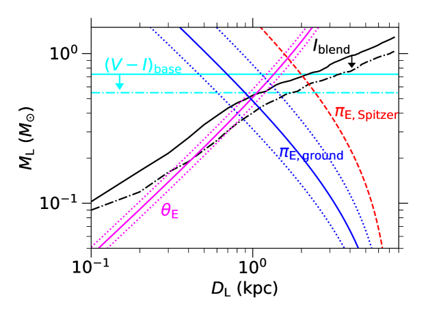
Figure 9: Constraints on the lens mass and distance. Magenta lines show the mass-distance relation calculated from $\theta_{\rm E}$ (solid) with the $1\sigma$ limits (dotted) for the $(s>1,u_{0}<0)$. Blue lines show the mass-distance relation and $1\sigma$ limits from the ground-based parallax for that solution (solid and dotted, respectively). Red, dashed line shows the mass-distance relation for $\pi_{\rm E}=0.25$, i.e., the best-fit value for the Spitzer-“only” parallax. The black lines are the $3\sigma$ upper limits derived from the blended light in I band. The cyan lines are the $3\sigma$ limits derived from the color of the baseline object. These give upper limits on the lens mass if it is behind all of the dust (solid) or in front (dot-dashed). Lenses below these lines are allowed.

Independent of any other constraints, the observed flux constrains the mass of the lens. First, there is a constraint from the blend flux. Because the blend consists of light from stars other than the lensed source (i.e., the lens and any other stars blended into the PSF), the lens cannot be brighter than the blend. In principle, because the background in the bulge consists of unresolved stars rather than blank sky, OGLE-2019-BLG-0960 could be sitting on a “hole” in the background (Park et al., 2004) and, therefore, the blend could be slightly brighter than measured. To place a $3\,\sigma$ upper limit on the flux from the lens, we take account of this effect in addition to the ordinary photon-based error in the measurement of the flux from the baseline object. These must be handled separately because the photon noise is Gaussian but the effect of the mottled background, including a possible “hole”, is highly non-Gaussian.

For the photon noise, we estimate the photometric error in the baseline object to be 0.020 mag. Subtracting the measured source flux (taking accont of its very small error), and propagating the errors, we find that this term contributes 0.0285 mag at $1\,\sigma$ and so 0.085 mag at $3\,\sigma$.

To account for the mottled background, we follow the method of Gould et al. (2020). We model the bulge stellar distribution using the Holtzman et al. (1998) luminosity function, scaled down by a factor 0.50 according the bulge projected clump-star density map of Nataf et al. (2013) and D. Nataf (2019, private communication). We estimate that OGLE-IV imaging captures field stars $I<20$ but leaves fainter stars unresolved, and that this map is constructed from FWHN$\sim 0.9^{\prime\prime}$ images. We then evaluate the impact of random field stars on the baseline-object (hence, blend) photometry by Monte Carlo. We find that at $(1,2,3)\sigma$ [i.e., (84.1,97.7,99.9) percentiles], the blend could be brighter than its naive value by (0.08,0.12,0.13) mag. Hence, the combined three sigma limit due to both photon noise and mottled background is 0.16 mag. Hence, the $3\,\sigma$ limit on the brightness of the lens is $I_{L}>18.38$.

Figure 9 shows the resulting limits on the lens mass and distance. For this figure, we have converted the limit on $I_{\rm L}$ to a limit on $M_{\rm L}$ using Pecaut & Mamajek (2013). To show the effect of dust, we have calculated these limits for both $I=18.38$ and $I_{0}=I-A_{I}=17.41$.

Second, the color of the baseline object provides an additional constraint on the lens. The baseline object (measured when the source is unmagnified) consists of light from the source, the lens, companions to those stars, and ambient stars blended into the PSF. We have measured the astrometic offset between the baseline object in higher-resolution CFHT imaging and the KMTNet microlensing event. We find $\Delta\theta_{\rm CFHT}=(23.1,7.6)\pm(12.2,18.4)\$ mas, which is consistent with zero offset. Hence, all or most of the light from the baseline object (and blend) is likely to be associated with the event as either the source, the lens, or a companion to one or both of them.

In this case, the baseline object in OGLE is very red: $(V-I)_{\rm base}=2.18\pm 0.13$. In the KMTC pyDIA CMD, the baseline object is the same, very red, color within errors. Because the source is blue relative to the clump, this necessarily implies that the blended light is at least as red or even redder than the baseline object. Hence, either the lens is also very red or it is much fainter than the blend. Even if the lens is behind all of the dust, this implies $(V-I)_{0,\rm L}>1.12$ at $3\sigma$, assuming $E(V-I)=0.67$. Then, using Pecaut & Mamajek (2013) to convert this color to a mass limit gives a limit of $M_{\rm L}\lesssim 0.73M_{\odot}$. This limit is shown in Figure 9 as is the limit for $(V-I)_{\rm L}>1.79$, which would imply the lens is in front of all of the dust.

5.3 Tension with Spitzer-“only” Parallax

If we combine the flux constraints on the mass of the lens with the measurement of $\theta_{\rm E}$, we can then place a constraint on the microlens parallax and the distance to the lens:

$$M_{\rm L}=\frac{\theta_{\rm E}}{\kappa\pi_{\rm E}};\quad\pi_{{\rm rel}}=\frac{\theta_{\rm E}^{2}}{\kappa M}=\left(\frac{{\rm AU}}{D_{\rm L}}-\frac{{\rm AU}}{D_{\rm S}}\right)$$ (6)

where we assume that the source is at the mean distance to the red clump, i.e., $D_{\rm S}=7.56\$ kpc. Given that $\theta_{*,0}\simeq 0.625\ \mu$as, the Einstein radius is quite large $\theta_{\rm E}=\theta_{*}/\rho\simeq 1.9\,{\rm mas}$. Hence, a mass limit of $M_{\rm L}<0.73\ M_{\odot}$ (from $(V-I)_{\rm base}$) implies $\pi_{\rm E}>0.32$ and $D_{\rm L}<1.35\$ kpc. However, this estimate is not fully self-consistent because, even if the lens were behind all of the dust, a $0.73\ M_{\odot}$ star at 1.35 kpc would be brighter than the observed blend (i.e., in Figure 9 the intersection of the cyan and magenta lines is above the black lines). Combining the blended light constraint with the $\theta_{\rm E}$ measurement results in an upper limit on the lens mass of $\sim 0.55\ M_{\odot}$, so $\pi_{\rm E}>0.42$ and $D_{\rm L}\lesssim 1\$kpc (intersection of the black and magenta lines in Figure 9).

From the ground-based parallax alone, we have a robust measurement of $\pi_{\rm E,\parallel}$. This gives a lower limit on the microlens parallax of $\pi_{\rm E}\gtrsim 0.3$. Combined with $\theta_{\rm E}$, $\pi_{\rm E,\parallel}$ alone implies $M_{\rm L}\lesssim 0.78M_{\odot}$. These limits are consistent with our expectations based on $\theta_{\rm E}$ and the blended light. The mass-distance relation calculated from the full ground-based $\pi_{\rm E}$ for the $(s>1,u_{0}<0)$ solution is shown in Figure 9 with $1\sigma$ limits. This shows that there are regions of overlap between this relation and the $\theta_{\rm E}$ relation that are consistent with the constraints from the blended light.

However, the constraints from the blend and baseline object support the conclusion that the low-amplitude signal in the Spitzer light curve should be treated with caution. The preferred value of the Spitzer-“only” parallax gives $\pi_{\rm E}=0.25$ (red line in Figure 9). This value is in tension with the ground-based parallax values at $\sim 3\sigma$, but, when combined with $\theta_{\rm E}$, it also implies $M_{\rm L}\simeq 0.93\ M_{\odot}$, which is too blue and too bright for the blended light. At the same time, the full $7\sigma$ arc from the Spitzer-“only” parallaxes includes regions that overlap with the ground-based parallax contours at $<2\sigma$ (see Figure 5) and which is also more compatible with the blended light. Thus, this tension may be resolved in the future once the constraints from the Spitzer light curve are better understood.

5.4 Physical Properties of the Lens

For now, we focus on constraints on the lens properties that may be derived from the ground-based analysis. Table 4 gives the physical properties of the lens derived from each solution to the microlensing light curve.

These values are both consistent with the constraints from the blended light and baseline object and suggest that the lens is responsible for most of the blend. For example, for the $(s>1),(u_{0}<0)$ solution, we have $M_{L}=0.50\pm 0.12M_{\odot}$ and $D_{\rm L}=0.98\pm 0.2$ kpc. For a 0.5 $M_{\odot}$ star, Pecaut & Mamajek (2013) give $M_{\rm I}=7.6$ and $(V-I)_{0}=2.0$. Hence, for a lens at 0.98 kpc,

$$I_{\rm L} = 17.6+A_{I}f_{\rm dust},$$ (7)

$$(V-I)_{\rm L} = 2.0+E(V-I)f_{\rm dust},$$ (8)

where $f_{\rm dust}$ is the fraction of the dust in front of the lens. We make the naive assumption that the dust follows an exponential profile such that $f_{\rm dust}=1-\exp(-D_{\rm L}/(1.334\ {\rm kpc}))$. Then, this yields $I_{\rm L}=18.07$ and $(V-I)_{\rm L}=2.35$, which is shown as the cyan point (“naive lens”) in Figure 8. The solid cyan line shows the values of $I_{\rm L}$ and $(V-I)_{\rm L}$ calculated for $\theta_{\rm E}=1.90\$ mas for the $1\sigma$ ranges for $\pi_{\rm E}$. The dotted lines show the results evaluated at $\theta_{\rm E}\pm 1\sigma$. Because of the simplified assumption about the dust, these calculations are simply meant to be illustrative. Nevertheless, they indicate that, within the uncertainties, the lens mass and distance are consistent with the blended light constraints within $1\sigma$ and suggest that the lens could be responsible for most or all of the blended light.

The hypothesis that the blend is the lens could be tested immediately with adaptive optics observations. These observations could give a stronger constraint associating the blended light with the event as well as a more precise measurement of that light by resolving out unrelated stars. Given the high lens-source relative proper motion ($\mu_{\rm rel}=11.4\pm 0.8\,{\rm mas\,yr^{-1}}$ or $\mu_{\rm rel}=12.2\pm 0.7\,{\rm mas\,yr^{-1}}$), it will be possible by $\sim 2025$ to separately resolve the source and lens (e.g., Terry et al., 2020), provided that the lens is responsible for a substantial fraction of the blended light. Such observations would confirm that the blended light is moving with the lens, i.e., that the separation matches the expectations from the lens-source relative proper motion given in Table 4. As discussed in Section 4, this would also give an independent measurement of the direction of that motion, which could be compared to the constraints from the parallax.

6 Discussion

OGLE-2019-BLG-0960Lb is the smallest mass-ratio microlensing planet ever found. With its discovery, there are now nineteen known planets with mass ratios below the fiducial break proposed by Suzuki et al. (2016), and four planets with mass ratios below the break found by Jung et al. (2019). Measuring the slope of the mass-ratio distribution below $q_{\rm br}$ requires a statistically robust sample, and while the current sample does not meet that criterion, it does offer insight into how such a sample might be obtained.

First, in Section 6.1, we consider whether or not the planetary perturbation can be characterized with only the survey data. Then, we note in Section 6.2 that most of the known microlensing planets with $q<10^{-4}$ have $s\sim 1$. We explore the implications of this for designing a search strategy for such planets, e.g., in either existing data or with targeted followup observations. Finally, we discuss in Section 6.3 the fact that $s\sim 1$ is far from the regime for which the $s\rightarrow 1/s$ degeneracy was derived, how the persistence of an $(s<1)$ vs. $(s>1)$ degeneracy suggests a deeper symmetry in the lens equation, and how the departure from the original ideal affects our ability to measure and interpret the mass-ratio function.

6.1 Characterization with Survey Data

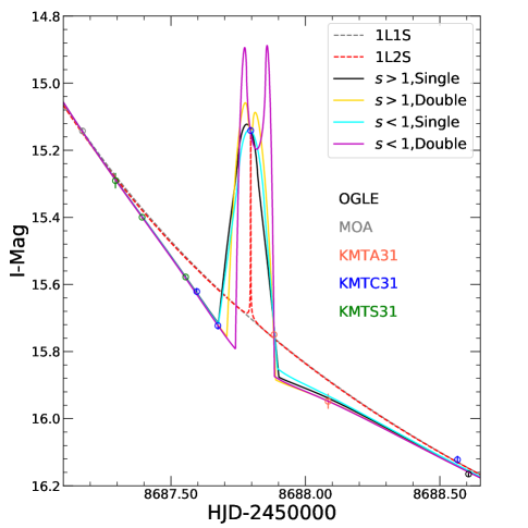
Figure 10: Zoom of the planetary perturbation for best-fit models to only the ground-based survey data. We recover the two solutions found when including all the data (“$s>1$, Single” and “$s<1$, Single”, black and cyan, respectively). However, the sparseness of the data allows two additional solutions to the light curve, with a much smaller source and two distinct caustic crossings (“$s>1$, Double” and “$s<1$, Double”, yellow and magenta, respectively). Nevertheless, the mass-ratio of the planet remains small for these solutions. The 1L2S solution (dashed red line) is still strongly ruled out by the survey data that are de-magnified relative to the 1L1S model (gray dashed line).

Naively, we would not expect such a small mass-ratio planet to be found in such a low-cadence survey field unless, as in this case, there are additional followup observations. Such planetary perturbations would typically last

$$t_{\rm p}\sim\sqrt{q}t_{\rm E}=4.8\ \mathrm{hr}\left(\frac{q}{10^{-4}}\right)^{1/2}\left(\frac{t_{\rm E}}{20\ \mathrm{d}}\right).$$ (9)

By contrast, all of the surveys observe this field at a cadence of less than one observation per hour (see Section 2). The highest survey cadence is for the MOA survey at $0.6\ \mathrm{hr}^{-1}$, which was not able to observe the night of the anomaly. Hence, the mass-ratio of this planet is an order of magnitude smaller than the expected minimum mass ratio for this field if we require 3 observations during the anomaly. Indeed, there is only a single survey observation over the main bump caused by the planet. However, because we know that the planet is real, we can ask whether this planet can be recovered and characterized with the sparse survey data (Yee et al., 2012). Then, we can consider whether or not this is evidence that short duration signals with only one to a few observations during the anomaly (the most likely case for the smallest planets) in general can be reliably and meaningfully recovered from sparse survey fields.

Therefore, we repeat the search for solutions using only the survey data (i.e., the data from OGLE, MOA, and KMTNet). The grid search over $s$, $q$, and $\alpha$ finds the previous two solutions but also a second pair of degenerate solutions (see Table 5 and Figure 2). The new set of solutions corresponds to the case in which the source is much smaller than the caustic and the single KMTC datapoint at 8687.796 falls in the trough between two caustic crossings (see Figure 10). Hence, this is an observational degeneracy that could be resolved with the addition of more data. Nevertheless, all four solutions lead to the same conclusions regarding the planetary parameters: the planetary perturbation is created by an extremely small mass-ratio planet at $s\sim 1$. We also find that the 1L2S solution is still strongly ruled out (by $\Delta\chi^{2}\sim 300$, see Table 3).

In some ways, it is not surprising that the planet parameters are so well constrained. Because observations are taken every $\sim 2.5\$hr, the maximum duration of the bump is $\sim 5\$ hr. Then, given Equation (9) and $t_{E}\sim 62\$ days, we would expect $q\lesssim 1.2\times 10^{-5}$. Then, the fact that the event does not produce a perturbation over the peak, despite the extremely high magnification, suggests a planetary caustic-like perturbation. At the same time, the perturbation occurs only 1.4 days after the peak, which places the “planetary” caustic very close to the central caustic, i.e., in a resonant or close-to-resonant configuration.

However, if the planetary perturbation were found and characterized based a single outlier, this would raise substantial questions as to the believability (or publishability) of the planet. In this case, we are fortunate to have extensive follow-up data, so the existence of the perturbation is well-supported. However, the detection of this planet in the survey data is strengthened by several other factors. First, this event has a longer timescale than average ($t_{\rm E}=62$ days), which enhances the duration of the perturbation via Equation (9), and hence, the likelihood of obtaining observations during the anomaly. Second, similar to KMT-2019-BLG-0842 (Jung et al., 2020), the source trajectory passes at an oblique angle with respect to the binary axis, which further lengthens the duration of the perturbation. As a result, we see from Figure 10 that there are five additional points that are significantly demagnified relative to the point-lens light curve. Hence, the perturbation lasts for almost a day and the detection does not, in fact, rely solely on a single outlier.

In terms of the broader implications for characterizing planetary perturbations based on sparse survey data, it is interesting to compare this event to other cases. The first such case was described in Dominik & Hirshfeld (1996), who showed that a number of different 2L1S models could explain two outliers in MACHO-LMC-001. Another case was described in Gaudi & Han (2004), who found multiple 2L1S models that fit a single outlier in OGLE-2002-BLG-055. One major contrast between these two events and OGLE-2019-BLG-0960 is the cadence of observations relative to the Einstein timescale. In both MACHO-LMC-001 and OGLE-2002-BLG-055, observations were only obtained once per few days during the perturbation, which allows for a much broader range of potential models. For example, the perturbation could always be much shorter, resulting in a relatively weak constraint on $q$ using Equation (9). Hence, even though the survey observations of OGLE-2019-BLG-0960 were relatively sparse compared to the duration of the perturbation, they are dense compared to $t_{\rm E}$, leading to good constraints on the planet. However, further investigation of short and sparsely-observed perturbations (but that might have well-constrained models) is needed to determine whether or not they are publishable in general.

6.2 Finding Small Mass-Ratio Planets

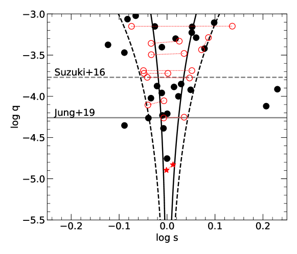
Figure 11: Known microlensing planets with $q<10^{-3}$ (NASA Exoplanet Archive, accessed 10/27/20). Solid points show planets with a single solution. Planets with multiple degenerate solutions are shown as open circles (one for each solution) connected by dotted lines (excludes planets with mass ratios that are ambiguous by more than a factor of 2). The two degenerate solutions for OGLE-2019-BLG-0960Lb are shown as the red stars. The gray lines show the fiducial $q_{\rm br}=1.7\times 10^{-4}$ as proposed by Suzuki et al. (2016) (dotted) and the value proposed by Jung et al. (2019) (solid). Black solid lines show the boundary between resonant and non-resonant caustics, and the dashed lines show $(3,1.8)\log s_{\rm resonant}$ for $(s<1)$ and $(s>1)$ caustic structures. The vast majority of planets are found between the dashed lines (so in resonant or close-to-resonant caustics, see Figure 12), and two are found at $\log s\sim 0.2$ in Hollywood events.

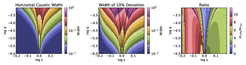
Figure 12: Left: The horizontal extent of the caustics; for non-resonant caustics, the extent is the sum of the widths of the planetary and central caustics. Center: The total extent of the region(s) along the binary axis that is perturbed by at least 10% relative to a point lens. The extents are measured as fractions of an Einstein ring. Right: Ratio of the 10% width to the caustic width. The black lines are as in Figure 11. The dashed lines were chosen to roughly correspond to the value of $s$ for which the extent of the 10% region is maximized at fixed $q$ (they are the same as those in Figure 11.). The range of $s$ over which the source plane is significantly perturbed by the planet is substantially larger than the range of $s$ for which the caustic size is maximized. Thus, the cross-section for a planetary perturbation to occur is substantially enhanced over the raw size of the caustics.

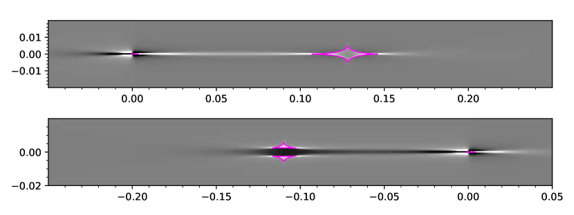
Figure 13: Maps showing the difference between the planetary magnification and the magnification of a point lens: $\log q=-4.85$ and $\log s=1.8\log s_{\rm resonant,wide}=0.0278$ (top) and $\log s=3\log s_{\rm resonant,close}=-0.0238$ (bottom). Planets just outside of resonance produce significant deviations to the point lens magnification extending between the two caustic structures (magenta), which may be either positive (white) or negative (black).

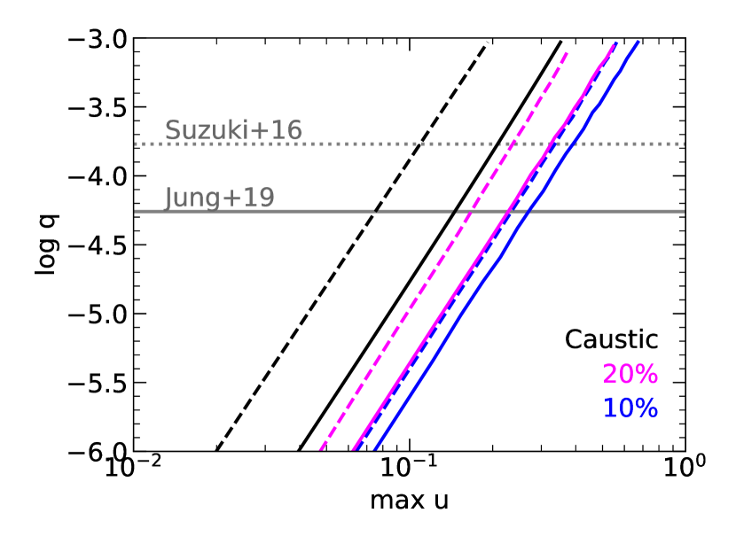
Figure 14: Black (dashed, solid): maximum radial extent “max u” of the $(s<1)$ and $(s>1)$ resonant caustic structures for a given value of $\log q$. Blue: maximum value of $|x|$ (which we use as a proxy for $u$) along the binary axis for which the magnification pattern is perturbed by at least 10% relative to a point lens. The value of $s$ is chosen such that the extent of the region is maximized for a given $q$ (see text, Figure 12). Magenta: same as blue but for a 20% perturbation. Gray lines as in Figure 11. Fully probing the region perturbed by the planet requires continuously monitoring the light curve through $\pm$ “max u”.

Given that there appear to be a number of factors that make this planetary perturbation “special,” we now consider how detections of small planets in general can be enhanced.

Previously, Abe et al. (2013) had suggested that the sensitivity of microlensing events to small planets was enhanced for moderate magnification events ($A>50$). Indeed, examining the published microlensing planets with $q<q_{\rm br}=1.7\times 10^{-4}$ supports this conclusion. Here, we include events with multiple degenerate solutions if all solutions are planetary and at least one solution has $q<q_{\rm br}$. Seven out of nineteen planets with $q<q_{\rm br}$ have been in events with $u_{0}\leq 0.02$ (i.e., $A\geq 50$). Another seven are found in events with $0.02<u_{0}\leq 0.1$ and two more in events with $0.1<u_{0}\leq 0.2$. The remaining three planets were all found in “Hollywood” events, in which the source was a giant.

The second thing to notice about the known small planets is that about half of them are found in events with resonant caustics and many of the others have separations that are close to resonance (see Figure 11 in which we exclude planets with ambiguous mass ratios, see caption). On the one hand, resonant caustics are larger than planetary caustics (the size of the resonant caustic scales as $q^{1/3}$ whereas the size of the planetary caustic scales as $q^{1/2}$; Dominik, 1998; Han, 2006), enhancing the probability that the images of the source are perturbed. On the other hand, resonant caustics are generally expected to produce weaker perturbations (Gaudi, 2012), which might not be significant enough to be detected. Empirically, Figure 11 shows that the majority of the detected planets are in resonant or near-resonant configurations, suggesting that the enhanced cross-section is the dominant effect and extends to configurations outside of resonance. It also suggests that the “enhancement” for detectability extends to planets with separations $s$ well outside the formal range for resonant caustics.

The enhanced cross-section for a perturbation for caustics close to, but outside of resonance, comes about because the perturbed magnification pattern extends out from and stretches all the way between the planetary and central caustics. Figure 12 compares the width of the caustics and the width of the region for which the magnification of a star+planet lens deviates by at least 10% compared to the star alone. For this exercise, we choose a 10% deviation as a reasonable threshold for producing a detectable perturbation. The “width of the caustics” is measured as the horizontal extent of the caustics (i.e., measured along the binary axis) and, if the caustic is not resonant, is the sum of the widths of the planetary and central caustics. The width of the deviation from a point lens is measured along a slice through the binary axis.

We usually think of the cross-section for detecting planetary perturbations as being equal to (or proportional to) the size of the caustics. However, Figure 12 shows that when measured in terms of a 10% deviation, the cross-section is largest for separations just outside of resonance and is significantly larger at that boundary than one would expect from strict proportionality. The decreased width of the 10% perturbation region for $\log s=0$ reflects the relative “weakness” of true resonant caustics. The maximum size of a 10% deviation for fixed $q$ peaks at $\sim 3\log s_{\rm resonant}$ for $s<1$ and $\sim 1.8\log s_{\rm resonant}$ for $s>1$, where $s_{\rm resonant}$ is the boundary between resonant and non-resonant caustics (i.e., Equations (57) and (58) from Dominik, 1998). Even though caustics in this region are not formally resonant, they are clearly influencing each other. Thus, we refer to caustics in this range as “semi-resonant.”

Abe et al. (2013) noted this effect for caustic structures with $s<1$ and referred to it as a “cooperative effect.” For such caustics, there is an extended “trough” (negative magnification deviation) along the binary axis connecting the planetary and central caustics (bottom panel of Figure 13). However, we also see this effect for $s>1$ caustics but in the form of a narrow “ridge” (positive magnification deviation) connecting the planetary and central caustics (top panel of Figure 13). These effects can also be seen in Figure 10 of Gaudi (2010). In terms of detectability, it may be that $s<1$ caustic perturbations are easier to detect because the vertical extent of the 10% deviation region is larger, and thus, a typical perturbation will last longer. Empirically, we do see that there are more $s<1$ planets than $s>1$ planets for $q<1.7\times 10^{-4}$, but the total numbers are still too small for this to be a statistically meaningful result. By contrast, Jung et al. (2020) noted that published perturbations crossing “ridges” found in $s>1$ events tend to have source trajectories with oblique angles. Such trajectories will result in proportionally longer perturbations, but represent only a small fraction of possible trajectories, suggesting many such perturbations are missed due to insufficient cadence.

In terms of detection strategy, Figure 14 shows the maximum value of $u$ for which the magnification pattern due to a planet is perturbed by at least 10% relative to a point lens. Because the orientation of the caustic structure relative to the source trajectory is random, this suggests that events should be monitored continuously for $\tau=\pm u$ in order to probe this full structure. In the case of OGLE-2019-BLG-0960, we called off the alert at $\tau\sim+0.01$, and thus, the planet was nearly missed. This investigation suggests that to search for planets with $\log q<-4.5$, events should be densely monitored for $\tau=\pm 0.2$, i.e. $A>5$. Indeed, Han et al. (2020) report the detection of a planet in KMT-2018-BLG-1025 with $q\sim 10^{-4}$ in which the perturbation occurred at $\tau\sim 0.05$.

6.3 “Close”/“Wide” Degeneracy for Semi-Resonant Caustics?

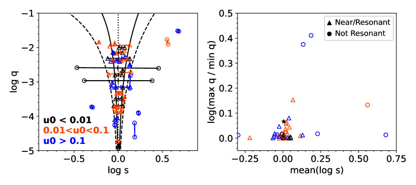
Figure 15: Left: microlensing planets with two degenerate solutions (NASA Exoplanet Archive, accessed 10/27/20). Dotted line at $\log s=0$, solid and dashed lines as in Figures 11 and 12. Points are colored by impact parameters, $u_{0}$, and the symbol types indicate whether the caustics are near-resonant/resonant (triangles) or non-resonant (circles), i.e., inside or outside the dashed lines. OGLE-2019-BLG-0960 is marked by black stars. Right: difference from a “true” “close”/“wide” degeneracy. Events with a perfect $s\leftrightarrow s^{-1}$ degeneracy should have mean$(\log s)\rightarrow 0$. By contrast, most of the events shown, including OGLE-2019-BLG-0960, have resonant or semi-resonant caustics (triangles), i.e., are not in the $|\log s|\gg 0$ regime, and many do not have mean$(\log s)\rightarrow 0$. For these events, the different degenerate solutions can have significant fractional deviations in $q$, in contrast to the expectation that $q$ is invariant to the “close”/“wide” degeneracy for the limit as $|\log s|\gg 0$.

Figure 11 also shows that many planets have multiple, degenerate solutions. These degenerate solutions usually have one solution with $s<1$ and another with $s>1$ and are often referred to as arising from the “close”/“wide” degeneracy. However, we will see that this degeneracy is more complex than the degeneracy that was first described by Griest & Safizadeh (1998) and expanded upon by Dominik (1998) and An (2005).

As an example, the two solutions for OGLE-2019-BLG-0960 nominally have the hallmarks of the “close”/“wide” degeneracy for central caustics. First, the event is in the “high-magnification” regime ($u_{0}<0.01$). Second, one of the solutions has $s<1$ while the other has $s>1$. However, the two solutions are not centered around $\log s=0$, i.e., $s_{\rm close}\neq s_{\rm wide}^{-1}$. Furthermore, the “close”/“wide” degeneracy was derived by Griest & Safizadeh (1998) and Dominik (1998) from the lensing equation in the regime where $|\log s|$ is large, i.e., the regime in which the central and planetary caustics are well-separated from each other. Griest & Safizadeh (1998) even state “We expect the formula to break down when $q\rightarrow 1$ or $x_{p}\rightarrow 1$” (where they use $x_{p}$ in place of $s$). OGLE-2019-BLG-0960  is clearly not in this regime: in both solutions, $s\sim 1$ and the caustic structure is resonant. Thus, it is interesting to consider whether this is in fact a case of the “close”/“wide” degeneracy.

Because the two solutions are not centered around $\log s=0$, they may in fact be more analogous to the “inner”/“outer” degeneracy described by (Calchi Novati et al., 2019) in which the source trajectory may pass either inside or outside the planetary caustic relative to the central caustic. An examination of the caustic structures for OGLE-2019-BLG-0960  (see Figure 3), shows that the “close” solution passes to the outside the caustic whereas the “wide” solution passes over the bridge in the resonant caustic created in between what would be the central and planetary caustics. Two other small planets, OGLE-2016-BLG-1195Lb and KMT-2019-BLG-0842Lb, also show this degeneracy (Bond et al., 2017; Shvartzvald et al., 2017; Jung et al., 2020).

The “inner”/“outer” degeneracy in these four events appears to result from the planetary caustic degeneracy that was first derived in the Chang-Refsdal limit (Chang & Refsdal, 1979) by Gaudi & Gould (1997). This degeneracy is intrinsic, i.e. rooted in mathematical symmetries in the lens equation rather than “accidental,” which refers to degeneracies arising due to insufficient observational coverage of the perturbation. However, again it was derived in the limit that $|\log s|$ was large, and it was expected to break down as $|\log s|\rightarrow 0$. None of these events is in the limit that $|\log s|$ is large, yet a degeneracy persists. This suggests that while the “close”/“wide” degeneracy of Griest & Safizadeh (1998) and the “inner”/“outer” degeneracy of Gaudi & Gould (1997) were derived in the limit that $|\log s|$ is large, as $|\log s|\rightarrow 0$, instead of breaking down, the two degeneracies merge.

To investigate this possibility in more detail, we review the known microlensing planets with two degenerate “geometric” solutions. These may refer to either two distinct caustic topologies or two distinct source trajectories relative to the caustic. As shown in Figure 15, of the planets with one $s<1$ and one $s>1$ solution, very few can be described as having well-separated caustics, i.e., are in the “close”/“wide” regime as described by Griest & Safizadeh (1998). The vast majority of planets with degenerate solutions are either in the resonant or semi-resonant regime, similar to OGLE-2019-BLG-0960.

Events in the resonant or semi-resonant regime share the characteristics that the degenerate solutions tend not to be perfectly symmetric about $|\log s|=0$. Also, in contrast to the Griest & Safizadeh (1998) limit, the degenerate solutions tend to have slightly different values of $q$. This is especially true for events in the moderate magnification regime ($0.01<u_{0}<0.1$), which is precisely the region where we expect the smallest planets to be found. Fortunately, because $|\log s|$ is very close to 0 in both cases, this degeneracy does not meaningfully affect the interpretation of the projected separation between the planet and its host star. However, the small differences in $q$ will have to be taken into account when interpreting statistical samples of such planets.

7 Conclusions

With a mass ratio of $q\sim 1.27\pm 0.07$ or $\sim 1.45\pm 0.15\times 10^{-5}$, OGLE-2019-BLG-0960Lb is the smallest mass-ratio microlensing planet ever found. The annual parallax effect combined with the finite source effect indicate the host star is an M-dwarf at $D_{\rm L}\lesssim 1\,$ kpc with a super-Earth planet orbiting between 1 and 2 au (see Table 4 for exact values for each solution). The lens is plausibly responsible for all or most of the blended light, a hypothesis that can be tested immediately by taking adaptive optics or HST observations to determine whether the blend is associated with the event.

OGLE-2019-BLG-0960Lb is the 19th microlensing planet with a mass-ratio below the fiducial power-law break in the mass-ratio distribution, $q_{\rm br}=1.7\times 10^{-4}$, posited by Suzuki et al. (2016). It is the fourth planet below the revised break of $q_{\rm br}=0.55\times 10^{-4}$ from Jung et al. (2019). The three smallest planets (including this one) have all been discovered since the advent of continuous survey observations from KMTNet. This indicates that the current generation of microlensing experiments is now capable of measuring both the precise location of $q_{\rm br}$ and the power-law slope, $p$, of the mass-ratio distribution below $q_{\rm br}$.

By comparing OGLE-2019-BLG-0960 with other published planets below $q_{\rm br}$ (Section 6.2), we found that they are primarily found in moderate magnification and “Hollywood” (Gould, 1997) events. Moderate magnification events are the primary source of small planets because the cross-section for a planetary perturbation is largest when the planetary caustics are near resonance. In fact, the planet sensitivity is maximized for planets just outside resonance ($|\log s|>|\log s_{\rm resonant}|$) because significant perturbations to the magnification field extend well beyond the caustic structures. However, the planet sensitivity decreases rapidly for $|\log s|\gtrsim{\rm few}|\log s_{\rm resonant}|$.

Three of the nineteen planets with mass ratios smaller than $q=1.7\times 10^{-4}$ were found in “Hollywood” events, for which the cross-section for light-curve anomalies is set by the source size rather than the caustic size. For these planets $s\gg s_{\rm resonant}$. The expected yield for such events is likely to be much lower than for moderate magnification events. Typical source sizes are $\rho\sim 0.01$, and thus, the cross-section is a factor of $\sim 10$ smaller than for moderate magnification events. At the same time, events with giant sources represent only a fraction of all microlensing events, making intensive work on such events tractable.

Hence, the focus for discovering planets with $\log q\lesssim-4$ should be on moderate magnification events and events with giant sources. This search could be conducted within existing survey data or be supplemented by a followup campaign. Even though OGLE-2019-BLG-0960Lb could be recovered from survey data alone (Section 6.1), this recovery was aided by the special geometry of the light curve (Jung et al., 2020) and suggests that similar, but shorter and potentially more numerous, perturbations would be missed in the low-cadence survey fields. For followup observations, Abe et al. (2013) previously suggested that the focus for small planets should be events with $50<A_{\rm max}<200$. Our investigation shows that events should be monitored for the full time that they have $A>5$, which suggests this focus should be extended to events with peak magnification $A_{\rm max}>10$ or even smaller. If additional resources are available, followup observations could be further extended to include events with giant sources. This strategy will maximize the number of small planets found and enable a robust measurement of the mass-ratio distribution of microlensing planets with $q<q_{\rm br}$.

Finally, OGLE-2019-BLG-0960 and many of the other planets in moderate magnification events suffer from a degeneracy that results in two solutions for the light curve: one with $s>1$ and one with $s<1$. For this event (and most small planets), such degeneracies have little effect on the interpretation of the separation of the planet from the host star, because $s\sim 1$. However, we showed in Section 6.3 that it does have some effect on the value of $q$. This is contrary to the expectation of Griest & Safizadeh (1998) that $q$ should be very similar under the “close”/“wide” degeneracy, likely because $s\sim 1$ is very far from the regime in which this degeneracy was derived. It seems likely that the origin of these degenerate solutions arises from some previously undiscovered symmetry in the lens equation of which the classical “close”/“wide” degeneracy may be a limiting case. However, truly understanding this symmetry requires going beyond the purely empirical investigation carried out in this paper.

Table 1: Data with corresponding data reduction method and rescaling factors

Collaboration	Site	Filter	Coverage (${\rm HJD}^{\prime}$)	$N_{\rm data}$	Reduction Method	$k$	$e_{\rm min}$
OGLE		$I$	7799.9 – 8763.6	488	Woźniak (2000)	1.27	0.000
OGLE		$V$	7851.9 – 8723.6	26	Woźniak (2000)	…	…
MOA		Red	8537.2 – 8785.9	341	Bond et al. (2001)	1.14	0.005
KMTNet	SSO	$I$	8682.0 – 8692.0	19	pySIS1	0.80	0.000
	CTIO	$I$	8616.7 – 8777.6	312	pySIS	1.33	0.007
	SAAO	$I$	8616.4 – 8777.3	223	pySIS	1.46	0.000
LCO	SSO01	$i$	8684.0 – 8690.2	147	ISIS2	2.03	0.005
	SSO02	$i$	8688.1 – 8691.9	46	ISIS	1.04	0.000
$\mu$FUN	CTIO	$i$	8684.6 – 8692.7	23	ISIS	…	…
$\mu$FUN	SAAO	$i$	8685.4 – 9690.2	91	ISIS	0.86	0.004
$\mu$FUN	CT13	$I$	8678.5 – 8692.7	65	DoPHOT3	1.12	0.000
$\mu$FUN	CT13	$H$	8678.5 – 8692.7	343	DoPHOT	…	…
$\mu$FUN	AO	540–700 nm	8685.9 – 8686.9	51	DoPHOT	1.29	0.000
$\mu$FUN	FCO	unfiltered	8685.9 – 8686.9	75	DoPHOT	0.82	0.000
$\mu$FUN	Kumeu	540–700 nm	8685.9 – 8687.9	108	DoPHOT	1.29	0.000
Spitzer		$L$	8685.2 – 8712.0	25	Calchi Novati et al. (2015)	1.98	0.000

¹ Albrow et al. (2009)
² Alard & Lupton (1998); Alard (2000); Zang et al. (2018)
³ Schechter et al. (1993)

Table 2: Parameters for 2L1S models using all ground-based data

Model	$\chi^{2}/dof$	$t_{0}$	$u_{0}$	$t_{\rm E}$	$s$	$q$	$\alpha$	$\rho$	$\pi_{\rm E,N}$	$\pi_{\rm E,E}$	$f_{\rm S,I}$	$f_{\rm B,I}$
		(${\rm HJD}^{\prime}$)		(d)		$(\times 10^{-5})$	(rad)	$(\times 10^{-4})$
$(s>1)$ :
Static	$2099.2/1935$	$8686.4484$	$0.0060$	$61.5$	$1.028$	$1.41$	$0.270$	$3.20$	…	…	$0.1781$	$0.5391$
		$0.0005$	$0.0001$	$1.4$	$0.001$	$0.14$	$0.001$	$0.17$	…	…	$0.0042$	$0.0037$
Parallax,	$1934.1/1933$	$8686.4490$	$0.0061$	$61.8$	$1.028$	$1.43$	$0.273$	$3.23$	$0.395$	$-0.393$	$0.1773$	$0.5385$
($u_{0}>0$)		$0.0006$	$0.0001$	$1.4$	$0.001$	$0.14$	$0.001$	$0.18$	$0.155$	$0.039$	$0.0041$	$0.0036$
Parallax,	$1932.0/1933$	$8686.4496$	$-0.0061$	$61.4$	$1.029$	$1.48$	$-0.272$	$3.29$	$-0.351$	$-0.313$	$0.1784$	$0.5380$
($u_{0}<0$)		$0.0006$	$0.0001$	$1.4$	$0.001$	$0.14$	$0.001$	$0.16$	$0.173$	$0.027$	$0.0041$	$0.0036$
$(s<1)$ :
Static	$2101.2/1935$	$8686.4485$	$0.0060$	$61.9$	$0.997$	$1.23$	$0.269$	$2.97$	…	…	$0.1769$	$0.5401$
		$0.0005$	$0.0001$	$1.3$	$0.001$	$0.06$	$0.001$	$0.09$	…	…	$0.0040$	$0.0040$
Parallax,	$1933.9/1933$	$8686.4487$	$0.0059$	$63.0$	$0.996$	$1.27$	$0.272$	$2.97$	$0.464$	$-0.405$	$0.1736$	$0.5418$
($u_{0}>0$)		$0.0005$	$0.0001$	$1.4$	$0.001$	$0.07$	$0.001$	$0.10$	$0.146$	$0.039$	$0.0042$	$0.0037$
Parallax,	$1933.0/1933$	$8686.4494$	$-0.0060$	$62.0$	$0.997$	$1.27$	$-0.271$	$3.01$	$-0.440$	$-0.304$	$0.1766$	$0.5397$
($u_{0}<0$)		$0.0005$	$0.0001$	$1.3$	$0.001$	$0.07$	$0.001$	$0.10$	$0.161$	$0.027$	$0.0039$	$0.0034$

Note: Uncertainties for each parameter are given in the second line for each solution.

Table 3: Parameters for 1L2S models using all ground-based data and ground-based survey data

Model	$\chi^{2}/dof$	$t_{0,1}$	$t_{0,2}$	$u_{0,1}$	$u_{0,2}$	$t_{\rm E}$	$\rho_{1}$	$\rho_{2}$	$\pi_{\rm E,N}$	$\pi_{\rm E,E}$	$q_{F,I}$	$f_{\rm S,I}$	$f_{\rm B,I}$
		(${\rm HJD}^{\prime}$)	(${\rm HJD}^{\prime}$)			(d)	$(\times 10^{-4})$	$(\times 10^{-4})$
All,	$2952.0/1931$	$8686.4425$	$8687.8064$	$0.0056$	$0.0003$	$66.1$	$9.5$	$3.1$	$0.341$	$-0.308$	$0.0054$	$0.1645$	$0.5501$
($u_{0}>0$)		$0.0005$	$0.0012$	$0.0004$	$0.0002$	$1.4$	$33.2$	$92.0$	$0.174$	$0.059$	$0.0028$	$0.0024$	$0.0028$
All,	$2951.4/1931$	$8686.4431$	$8687.8076$	$-0.0056$	$-0.0003$	$65.6$	$6.4$	$3.0$	$-0.234$	$-0.233$	$0.0053$	$0.1656$	$0.5499$
($u_{0}<0$)		$0.0005$	$0.0011$	$0.0004$	$0.0002$	$1.3$	$30.2$	$82.1$	$0.370$	$0.079$	$0.0025$	$0.0022$	$0.0026$
Survey,	$1616.0/1323$	$8686.4406$	$8687.7951$	$0.0065$	$0.0000$	$66.3$	$61.4$	$0.1$	$-0.051$	$-0.224$	$0.0001$	$0.1641$	$0.5510$
($u_{0}>0$)		$0.0017$	$0.0116$	$0.0003$	$0.3024$	$0.5$	$13.4$	$273.3$	$0.299$	$0.053$	$0.0009$	$0.0166$	$0.0172$
Survey,	$1614.9/1323$	$8686.4386$	$8687.7953$	$-0.0057$	$-0.0000$	$67.2$	$33.4$	$0.1$	$-0.622$	$-0.244$	$0.0001$	$0.1614$	$0.5545$
($u_{0}<0$)		$0.0018$	$0.0126$	$0.0003$	$0.3401$	$0.5$	$17.1$	$265.0$	$0.387$	$0.070$	$0.0008$	$0.0171$	$0.0180$

Table 4: Physical parameters

Model	$\theta_{\rm E}$	$\pi_{\rm E}$	$\mu_{\rm rel}$	$M_{\rm L}$	$D_{\rm L}$	$m_{p}$	$a_{\perp}$
	(mas)		(${\rm mas\,yr^{-1}}$)	($M_{\odot}$)	(kpc)	($M_{\oplus}$)	(AU)
$(s>1)$ :
($u_{0}>0$)	$1.93\pm 0.13$	$0.557\pm 0.125$	$11.4\pm 0.8$	$0.43\pm 0.10$	$0.83\pm 0.17$	$2.0\pm 0.5$	$1.65\pm 0.35$
($u_{0}<0$)	$1.90\pm 0.12$	$0.470\pm 0.114$	$11.3\pm 0.8$	$0.50\pm 0.12$	$0.98\pm 0.21$	$2.5\pm 0.6$	$1.90\pm 0.43$
$(s<1)$ :
($u_{0}>0$)	$2.09\pm 0.11$	$0.616\pm 0.126$	$12.1\pm 0.7$	$0.42\pm 0.09$	$0.70\pm 0.13$	$1.8\pm 0.4$	$1.45\pm 0.28$
($u_{0}<0$)	$2.07\pm 0.11$	$0.535\pm 0.121$	$12.2\pm 0.7$	$0.48\pm 0.11$	$0.81\pm 0.17$	$2.0\pm 0.5$	$1.67\pm 0.37$

Table 5: Best-fit parameters for the four solutions using only ground-based survey data

Model	$\chi^{2}/dof$	$t_{0}$	$u_{0}$	$t_{\rm E}$	$s$	$q$	$\alpha$	$\rho$	$\pi_{\rm E,N}$	$\pi_{\rm E,E}$	$f_{\rm S,I}$	$f_{\rm B,I}$
		(${\rm HJD}^{\prime}$)		(d)		$(\times 10^{-5})$	(rad)	$(\times 10^{-4})$
$(s>1)$ :
Single	$1325.3/1324$	$8686.4504$	$0.0059$	$62.6$	$1.027$	$1.41$	$0.271$	$3.12$	$0.093$	$-0.352$	$0.1747$	$0.5408$
		$0.0022$	$0.0002$	$1.5$	$0.007$	$0.16$	$0.002$	$0.28$	$0.288$	$0.046$	$0.0043$	$0.0037$
Double	$1323.8/1324$	$8686.4513$	$0.0060$	$62.0$	$1.028$	$1.69$	$0.269$	$1.75$	$0.032$	$-0.334$	$0.1767$	$0.5390$
		$0.0021$	$0.0002$	$1.1$	$0.004$	$0.32$	$0.003$	$0.63$	$0.293$	$0.047$	$0.0033$	$0.0030$
$(s<1)$ :
Single	$1325.2/1324$	$8686.4506$	$0.0059$	$62.6$	$0.994$	$1.43$	$0.269$	$3.26$	$0.081$	$-0.351$	$0.1748$	$0.5407$
		$0.0016$	$0.0002$	$1.4$	$0.007$	$0.20$	$0.002$	$0.25$	$0.351$	$0.042$	$0.0042$	$0.0037$
Double	$1323.3/1324$	$8686.4522$	$0.0060$	$61.3$	$0.994$	$1.89$	$0.264$	$0.78$	$0.077$	$-0.332$	$0.1787$	$0.5373$
		$0.0027$	$0.0001$	$1.1$	$0.007$	$0.37$	$0.004$	$0.30$	$0.301$	$0.046$	$0.0031$	$0.0028$

References

- Abe et al. (2013) Abe, F., Airey, C., Barnard, E., et al. 2013, ArXiv e-prints, arXiv:1303.4123
- Adams et al. (2018) Adams, A. D., Boyajian, T. S., & von Braun, K. 2018, MNRAS, 473, 3608
- Alard (2000) Alard, C. 2000, A&AS, 144, 363
- Alard & Lupton (1998) Alard, C., & Lupton, R. H. 1998, ApJ, 503, 325
- Albrow et al. (2009) Albrow, M. D., Horne, K., Bramich, D. M., et al. 2009, MNRAS, 397, 2099
- An (2005) An, J. H. 2005, MNRAS, 356, 1409
- Batista et al. (2015) Batista, V., Beaulieu, J. P., Bennett, D. P., et al. 2015, ApJ, 808, 170
- Batista et al. (2011) Batista, V., Gould, A., Dieters, S., et al. 2011, A&A, 529, A102+
- Bennett et al. (2015) Bennett, D. P., Bhattacharya, A., Anderson, J., et al. 2015, ApJ, 808, 169
- Bensby et al. (2011) Bensby, T., Adén, D., Meléndez, J., et al. 2011, A&A, 533, A134+
- Bhattacharya et al. (2020) Bhattacharya, A., Bennett, D. P., Beaulieu, J. P., et al. 2020, arXiv e-prints, arXiv:2009.02329
- Bond et al. (2001) Bond, I. A., Abe, F., Dodd, R. J., et al. 2001, MNRAS, 327, 868
- Bond et al. (2017) Bond, I. A., Bennett, D. P., Sumi, T., et al. 2017, MNRAS, 469, 2434
- Bozza (2010) Bozza, V. 2010, MNRAS, 408, 2188
- Calchi Novati et al. (2015) Calchi Novati, S., Gould, A., Yee, J. C., et al. 2015, ApJ, 814, 92
- Calchi Novati et al. (2019) Calchi Novati, S., Suzuki, D., Udalski, A., et al. 2019, AJ, 157, 121
- Cassan et al. (2012) Cassan, A., Kubas, D., Beaulieu, J.-P., et al. 2012, Nature, 481, 167
- Chang & Refsdal (1979) Chang, K., & Refsdal, S. 1979, Nature, 282, 561
- Claret & Bloemen (2011) Claret, A., & Bloemen, S. 2011, A&A, 529, A75
- DePoy et al. (2003) DePoy, D. L., Atwood, B., Belville, S. R., et al. 2003, Society of Photo-Optical Instrumentation Engineers (SPIE) Conference Series, Vol. 4841, A Novel Double Imaging Camera (ANDICAM), ed. M. Iye & A. F. M. Moorwood, 827–838
- Dominik (1998) Dominik, M. 1998, A&A, 329, 361
- Dominik (1999) —. 1999, A&A, 349, 108
- Dominik & Hirshfeld (1996) Dominik, M., & Hirshfeld, A. C. 1996, A&A, 313, 841
- Dong et al. (2009) Dong, S., Gould, A., Udalski, A., et al. 2009, ApJ, 695, 970
- Foreman-Mackey et al. (2013) Foreman-Mackey, D., Hogg, D. W., Lang, D., & Goodman, J. 2013, PASP, 125, 306
- Gaudi (1998) Gaudi, B. S. 1998, ApJ, 506, 533
- Gaudi (2010) —. 2010, ArXiv e-prints, arXiv:1002.0332
- Gaudi (2012) —. 2012, ARA&A, 50, 411
- Gaudi & Gould (1997) Gaudi, B. S., & Gould, A. 1997, ApJ, 477, 152
- Gaudi & Han (2004) Gaudi, B. S., & Han, C. 2004, ApJ, 611, 528
- Gould (1994) Gould, A. 1994, ApJ, 421, L71
- Gould (1997) Gould, A. 1997, in Variables Stars and the Astrophysical Returns of the Microlensing Surveys, ed. R. Ferlet, J.-P. Maillard, & B. Raban, 125
- Gould (2004) —. 2004, ApJ, 606, 319
- Gould et al. (1994) Gould, A., Miralda-Escude, J., & Bahcall, J. N. 1994, ApJ, 423, L105
- Gould et al. (2010) Gould, A., Dong, S., Gaudi, B. S., et al. 2010, ApJ, 720, 1073
- Gould et al. (2020) Gould, A., Ryu, Y.-H., Calchi Novati, S., et al. 2020, Journal of Korean Astronomical Society, 53, 9
- Griest & Safizadeh (1998) Griest, K., & Safizadeh, N. 1998, ApJ, 500, 37
- Han (2006) Han, C. 2006, ApJ, 638, 1080
- Han et al. (2020) Han, C., Udalski, A., Lee, C.-U., & et al. 2020, A&A, submitted
- Hirao et al. (2020) Hirao, Y., Bennett, D. P., Ryu, Y.-H., et al. 2020, AJ, 160, 74
- Holtzman et al. (1998) Holtzman, J. A., Watson, A. M., Baum, W. A., et al. 1998, AJ, 115, 1946
- Jung et al. (2019) Jung, Y. K., Gould, A., Zang, W., et al. 2019, AJ, 157, 72
- Jung et al. (2020) Jung, Y. K., Udalski, A., Zang, W., et al. 2020, AJ, 160, 255
- Kim et al. (2018) Kim, H.-W., Hwang, K.-H., Shvartzvald, Y., et al. 2018, arXiv e-prints, arXiv:1806.07545
- Kim et al. (2016) Kim, S.-L., Lee, C.-U., Park, B.-G., et al. 2016, Journal of Korean Astronomical Society, 49, 37
- Minniti et al. (2017) Minniti, D., Lucas, P., & VVV Team. 2017, VizieR Online Data Catalog, II/348
- Nataf et al. (2013) Nataf, D. M., Gould, A., Fouqué, P., et al. 2013, ApJ, 769, 88
- Nataf et al. (2016) Nataf, D. M., Gonzalez, O. A., Casagrande, L., et al. 2016, MNRAS, 456, 2692
- Paczynski (1986) Paczynski, B. 1986, ApJ, 304, 1
- Park et al. (2004) Park, B. G., DePoy, D. L., Gaudi, B. S., et al. 2004, ApJ, 609, 166
- Pecaut & Mamajek (2013) Pecaut, M. J., & Mamajek, E. E. 2013, ApJS, 208, 9
- Refsdal (1966) Refsdal, S. 1966, MNRAS, 134, 315
- Schechter et al. (1993) Schechter, P. L., Mateo, M., & Saha, A. 1993, PASP, 105, 1342
- Shvartzvald et al. (2017) Shvartzvald, Y., Yee, J. C., Calchi Novati, S., et al. 2017, ApJ, 840, L3
- Skowron et al. (2011) Skowron, J., Udalski, A., Gould, A., et al. 2011, ApJ, 738, 87
- Smith et al. (2003) Smith, M. C., Mao, S., & Paczyński, B. 2003, MNRAS, 339, 925
- Street et al. (2016) Street, R. A., Udalski, A., Calchi Novati, S., et al. 2016, ApJ, 819, 93
- Suzuki et al. (2016) Suzuki, D., Bennett, D. P., Sumi, T., et al. 2016, ApJ, 833, 145
- Terry et al. (2020) Terry, S. K., Bhattacharya, A., Bennett, D. P., et al. 2020, arXiv e-prints, arXiv:2009.08461
- Udalski (2003) Udalski, A. 2003, Acta Astron., 53, 291
- Udalski et al. (2015) Udalski, A., Szymański, M. K., & Szymański, G. 2015, Acta Astron., 65, 1
- Udalski et al. (2005) Udalski, A., Jaroszyński, M., Paczyński, B., et al. 2005, ApJ, 628, L109
- Udalski et al. (2018) Udalski, A., Ryu, Y. H., Sajadian, S., et al. 2018, Acta Astron., 68, 1
- Vandorou et al. (2020) Vandorou, A., Bennett, D. P., Beaulieu, J.-P., et al. 2020, AJ, 160, 121
- Woźniak (2000) Woźniak, P. R. 2000, Acta Astronomica, 50, 421
- Yang et al. (2020) Yang, H., Zhang, X., Hwang, K.-H., et al. 2020, AJ, 159, 98
- Yee et al. (2009) Yee, J. C., Udalski, A., Sumi, T., et al. 2009, ApJ, 703, 2082
- Yee et al. (2012) Yee, J. C., Shvartzvald, Y., Gal-Yam, A., et al. 2012, ApJ, 755, 102
- Yee et al. (2015) Yee, J. C., Gould, A., Beichman, C., et al. 2015, ApJ, 810, 155
- Yoo et al. (2004) Yoo, J., DePoy, D. L., Gal-Yam, A., et al. 2004, ApJ, 616, 1204
- Zang et al. (2018) Zang, W., Penny, M. T., Zhu, W., et al. 2018, PASP, 130, 104401
- Zang et al. (2020) Zang, W., Shvartzvald, Y., Udalski, A., et al. 2020, ApJ, 891, 3