Automated 3D cephalometric landmark identification using computerized tomography

Abstract

Identification of 3D cephalometric landmarks that serve as proxy to the shape of human skull is the fundamental step in cephalometric analysis. Since manual landmarking from 3D computed tomography (CT) images is a cumbersome task even for the trained experts, automatic 3D landmark detection system is in a great need. Recently, automatic landmarking of 2D cephalograms using deep learning (DL) has achieved great success, but 3D landmarking for more than 80 landmarks has not yet reached a satisfactory level, because of the factors hindering machine learning such as the high dimensionality of the input data and limited amount of training data due to ethical restrictions on the use of medical data. This paper presents a semi-supervised DL method for 3D landmarking that takes advantage of anonymized landmark dataset with paired CT data being removed. The proposed method first detects a small number of easy-to-find reference landmarks, then uses them to provide a rough estimation of the entire landmarks by utilizing the low dimensional representation learned by variational autoencoder (VAE). Anonymized landmark dataset is used for training the VAE. Finally, coarse-to-fine detection is applied to the small bounding box provided by rough estimation, using separate strategies suitable for mandible and cranium. For mandibular landmarks, patch-based 3D CNN is applied to the segmented image of the mandible (separated from the maxilla), in order to capture 3D morphological features of mandible associated with the landmarks. We detect 6 landmarks around the condyle all at once, instead of one by one, because they are closely related to each other. For cranial landmarks, we again use VAE-based latent representation for more accurate annotation. In our experiment, the proposed method achieved an averaged 3D point-to-point error of 2.91 mm for 90 landmarks only with 15 paired training data.

1 Introduction

Cephalometric analysis is commonly used by dentists, orthodontists, and oral and maxillofacial surgeons to provide morphometrical guidelines for diagnosis, surgical planning, growth analysis, and treatment planning by analyzing dental and skeletal relationships in the craniofacial complex [Tenti1981]. It is based on cephalometric landmarks, which serve as proxy to the skull morphological data pertaining to craniofacial characteristics [Proffit2018]. Conventional cephalometric analysis uses two-dimensional (2D) cephalometric radiographs (lateral and frontal radiographs), which have drawbacks including geometric distortions, superimpositions, and the dependence on correct head positioning [Pittayapat2014]. Due to recent advances in image processing techniques and the need for accurate craniofacial analysis, a three-dimensional (3D) approach to the cephalometric landmarks obtaining 3D computerized tomography (CT) images is gaining preference over the conventional 2D techniques [Adams2004, Nalcaci2010, Lee2014].

Recently, there have been many studies conducted on automated cephalometric landmark identification that aim to find the landmarks and enable immediate cephalometric analysis, because manual landmarking and cephalometric analysis are labor-intensive and cumbersome tasks even for the trained experts. Due to recent advances in deep learning techniques, the automated annotation of 2D cephalometric landmarks may now be used for clinical application [Arik2017, Lindner2016]. Conversely, automated 3D cephalometric tracing (for 90 landmarks) may not yet be utilized in clinical applications, wherein the required average error is commonly designated to be less than 2 mm [Codari2017, Montufar2018, Lee2019, Kang2020, Yun2020]. The high dimensionality of the input data (e.g., $512\times 512\times 512$) and limited number of training data are the main factors that hinder the training of deep learning networks for learning the 3D landmark positional vectors from 3D CT data. Moreover, due to the current legal and ethical restrictions on medical data, it is very difficult to utilize CT data from patients.

To overcome the above-mentioned learning problems caused by the high input dimensions and training data deficiencies, the method proposed in this study utilizes semi-supervised learning that takes advantage of a large number of anonymized landmark dataset (without using the corresponding CT dataset) which have been used in surgical planning and treatment evaluation. We use these landmark dataset to obtain their low dimensional representations, reducing the dimensions of the total landmark vectors ($270=90\times 3$ dimension) to only 9 latent variables via a variational autoencoder (VAE) [Kingma2013]. For training the VAE, a normalized landmark dataset is used to efficiently learn skull shape variations while ignoring unnecessary scaling factors. With this dimensionality reduction technique, the positions of all 90 landmarks can be roughly estimated by identifying a small number of easy-to-find reference landmarks (10 landmarks), which can be accurately and reliably identified via a simple deep learning method [Lee2019].

The rough estimation of all landmarks is used to provide a small 3D bounding box for each landmark in the 3D CT images. Following this, we apply convolutional neural networks (CNNs) to these small bounding boxes to enable the accurate placement of landmarks. Our fine detection strategy is divided into two parts: mandible and cranium. It is desirable to accurately capture the morphological variability of the mandible because the shape of the mandible can be affected by a variety of factors, including the masticatory occlusal force, muscular force, functional activity such as breathing and swallowing, and age [Vallabh2019]. Noting that landmarks on the mandible represent morphological features of a 3D mandibular surface geometry, we apply 3D CNN to a segmented image of the mandible (separated from the cranium). We refer to the recent study [Jang2020] for a segmentation method to separate the mandible from the cranium.

Because several landmarks around the condyle are closely related to each other, it is better to detect these landmarks all at once. For the landmarks on the midsagittal plane, it is better to further reduce the dimensionality of the input by using a partially integrated 2D image of the midsagittal plane. For the remaining landmarks lying on the cranium, we again use the anonymized landmark dataset to obtain a more accurate latent representation of all landmarks on the cranium, due to its rigidity. The proposed approach achieved an average 3D point-to-point error of 2.91 mm for 90 landmarks, which nearly meets the clinically acceptable precision standard. It should be emphasized that this accuracy has been achieved using a very small amount of training data.

2 Method

For ease of explanation, we begin by introducing the following notations. Five easy-to-find reference landmarks (CFM, Bregma, Na, and Po (L/R)) are used as the basis for constructing a coordinate system to determine the midsagittal and axial planes, and they were utilized for data normalization (methods for obtaining these five reference landmarks will be described in Section 2.1).

• $\boldsymbol{x}$ denotes a 3D CT image, which is defined on a voxel grid $\Omega:=\{v=(v_{1},v_{2},v_{3}):v_{j}=1,\cdots,512\mbox{ for }j=1,2,3\}$. Here, we set $v_{1}$ as the normal direction of the midsagittal plane.

• $\boldsymbol{x}_{b}$ denotes a binarized CT image of $\boldsymbol{x}$, defined by

  $$\boldsymbol{x}_{b}=\left\{\begin{array}[]{cl}\boldsymbol{x}_{b}(v_{1},v_{2},v_{3})=1&\mbox{ if }\boldsymbol{x}(v_{1},v_{2},v_{3})\geq\rho\\ \boldsymbol{x}_{b}(v_{1},v_{2},v_{3})=0&\mbox{ otherwise }\end{array}\right.$$ (1)

  where $\rho$ is a thresholding value.

• $\boldsymbol{x}^{\mbox{\tiny mid}}$ denotes a partially integrated 2D image of $\boldsymbol{x}_{b}$ in the normal direction of the midsagittal plane, defined by

  $$\boldsymbol{x}^{\mbox{\tiny mid}}=\sum_{v_{1}=a}^{b}\boldsymbol{x}_{b}(v_{1},v_{2},v_{3})$$ (2)

  where $[a,b]$ determines the truncated volume of $\boldsymbol{x}_{b}$.

• $\mathfrak{R}^{\mbox{\tiny cr}}\in\mathbb{R}^{138(=46\times 3)}$ and $\mathfrak{R}^{\mbox{\tiny md}}\in\mathbb{R}^{132(=44\times 3)}$ denote the concatenated vectors of 46 cranial and 44 mandibular 3D landmarks, respectively. The entirety of the landmarks $\mathfrak{R}\in\mathbb{R}^{270(=90\times 3)}$ is defined by $\mathfrak{R}:=[\mathfrak{R}^{\mbox{\tiny cr}},\mathfrak{R}^{\mbox{\tiny md}}]$. See A for more detailed information of the landmarks.

• $\mathfrak{R}^{\mbox{\tiny cr}}_{\sharp}\in\mathbb{R}^{24(=8\times 3)}$ denotes a concatenated vector of landmarks (Bregma, CFM, Na, ANS, Or (L/R), and Po (L/R)) in the cranium and $\mathfrak{R}^{\mbox{\tiny md}}_{\sharp}\in\mathbb{R}^{6(=2\times 3)}$ denotes a concatenated vector of landmarks (MF (L/R)) in the mandible. A reference landmark vector $\mathfrak{R}_{\sharp}\in\mathbb{R}^{30(=10\times 3)}$ is defined by $\mathfrak{R}_{\sharp}=[\mathfrak{R}^{\mbox{\tiny cr}}_{\sharp},\mathfrak{R}^{\mbox{\tiny md}}_{\sharp}]$.

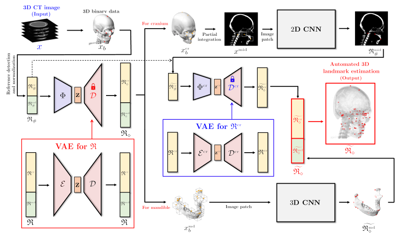
Figure 1: Schematic diagram of the proposed method for the 3D landmark annotation system.

The 3D cephalometric landmarking aims to develop a function $f:\boldsymbol{x}\mapsto\mathfrak{R}$ that maps from a 3D CT image $\boldsymbol{x}$ to all landmarks $\mathfrak{R}$. To learn the landmark detection map $f$, deep learning techniques can be used. Unfortunately, due to legal and ethical restrictions on medical data, a few paired data are available. This severe shortage of paired data makes it difficult to obtain an accurate and reliable map $f:\boldsymbol{x}\mapsto\mathfrak{R}$ in the following supervised learning framework:

$$f=\underset{f\in{\mathbb{N}}\mbox{\scriptsize et}}{\mbox{argmin}}\frac{1}{N_{p}}\sum_{i=1}^{N_{p}}\|f(\boldsymbol{x}^{(i)})-\mathfrak{R}^{(i)}\|^{2}_{2},$$ (3)

where $N_{p}$ is the small number of paired training data, $\{(\boldsymbol{x}^{(i)},\mathfrak{R}^{(i)}):i=1,\cdots,N_{p}\}$ is a paired dataset, ${\mathbb{N}}\mbox{et}$ is a deep learning network, and $\|\cdot\|$ is the standard Euclidean norm. In our study, only 15 paired data are available (i.e., $N_{p}=15$). Even with a certain amount of paired data, the learning process (3) of the direct detection map $f$ can be difficult because the dimension of the input image is very large (greater than 100,000,000).

The proposed method attempts to address this problem by taking advantage of a semi-supervised learning framework that permits the utilization of the $N_{l}$ number of anonymized landmark data $\{\mathfrak{R}^{(N_{p}+i)}\}_{i=1}^{N_{l}}$ whose corresponding CT data are not provided. As shown in Figure 1, the proposed method comprises the following three main steps: (i) To obtain easy-to-find reference landmarks $\mathfrak{R}_{\sharp}$, we apply CNN with 2D illuminated images generated from a binarized CT image $\boldsymbol{x}_{b}$ and normalize the output with respect to the cranial volume. (ii) A rough estimation of entire landmarks $\mathfrak{R}$ is obtained using the partial knowledge $\mathfrak{R}_{\sharp}$ and a VAE-based low dimensional representation of $\mathfrak{R}$. (iii) Using this estimation, coarse-to-fine detection for $\mathfrak{R}$ is conducted, wherein separate strategies are utilized for the mandibular and cranial landmarks. For the mandibular landmarks, the landmarks are accurately identified by applying 3D patch-based CNNs to capture the morphological features on a 3D surface geometry associated with the landmarks, wherein an input patch is extracted based on the coarse estimation. For cranial landmarks, we first detect three landmarks lying on the midsagittal plane by applying a 2D CNN whose input is an extracted 2D patch from a partially integrated image $\boldsymbol{x}^{\mbox{\tiny mid}}$ in basis of the coarse estimation. By utilizing the three finely-detected landmarks and cranial reference landmarks $\mathfrak{R}^{\mbox{\tiny cr}}_{\sharp}$ as the partial information of $\mathfrak{R}^{\mbox{\tiny cr}}$, the remaining cranial landmarks are finely annotated via a VAE-based local-to-global estimation utilizing the same method in the previous step .

Each of these steps is described in detail as follows.

2.1 Detection of easy-to-find reference landmarks and uniform scaling for skull normalization with respect to the cranial volume

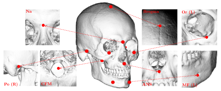
Figure 2: Reference landmarks. These are easy-to-find through CNN with input of the illuminated images because they have strong geometric cues that can be revealed in illuminated 2D images.

The first step of the proposed method is to find 10 reference landmarks $\mathfrak{R}_{\sharp}$ from a given $\boldsymbol{x}$. Initially, a CT image $\boldsymbol{x}$ is converted into a binarized image $\boldsymbol{x}_{b}$ by (1). From $\boldsymbol{x}_{b}$, 2D illuminated images are generated by manipulating various lighting and viewing directions (see Figure 2). By applying VGGNet [Simonyan2014] to these illuminated images, the reference landmarks $\mathfrak{R}_{\sharp}$ are accurately and automatically identified. This detection method is based on that presented in the recent study [Lee2019].

Using these identified reference landmarks, data normalization is conducted for efficient feature learning of skull shape variations in further steps. By applying uniform scaling with respect to the cranial volume, the landmark vector $\mathfrak{R}_{\sharp}$ is normalized, wherein the cranial volume is defined via a product of the distance between the $v_{1}$-coordinate of Po (L) and Po (R) (cranial length), the distance between the $v_{2}$-coordinate of Po (L) and Na (depth), and the distance between the $v_{3}$-coordinate of CFM and Bregma (height). This data normalization minimizes the positional dependencies of landmarks on the translation, rotation, and overall size of the skull; therefore, shape information of the skull (regarding facial deformities) can be effectively learned in further VAE-based steps. From here on, we will denote all landmark vectors as normalized vectors (e.g., $\mathfrak{R}$ and $\mathfrak{R}_{\sharp}$ are normalized vectors for total landmarks and reference landmarks).

2.2 Rough estimation of all landmarks from reference landmarks using VAE-based low dimensional representation

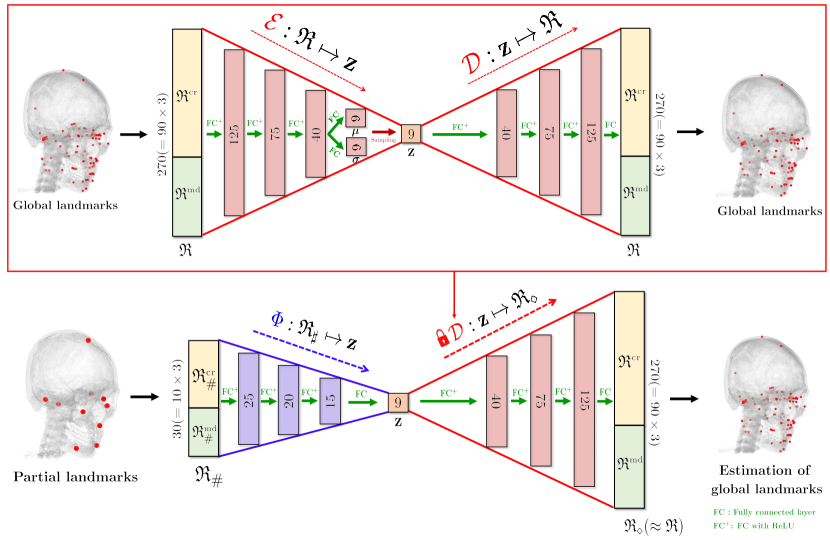
Figure 3: Initial estimation of all 90 landmarks $\mathfrak{R}$ using the knowledge of 10 reference landmarks $\mathfrak{R}_{\sharp}$. This is possible because all landmarks $\mathfrak{R}$ can be roughly represented by only 9 latent variables.

This section provides a method for roughly estimating all landmarks $\mathfrak{R}$ from the reference landmarks $\mathfrak{R}_{\sharp}$ that are accurately annotated in the previous step. Based on the method in [Yun2020], we build a bridge that connects $\mathfrak{R}_{\sharp}$ and $\mathfrak{R}$ by taking advantage of a low dimensional representation of $\mathfrak{R}$ learned by a variational autoencoder (VAE) [Kingma2013].

The rough estimation obtained from $\mathfrak{R}_{\sharp}$, denoted by $\mathfrak{R}_{\diamond}$, is given by

$$\mathfrak{R}_{\diamond}=\mathcal{D}\circ\Phi(\mathfrak{R}_{\sharp})$$ (4)

where $\mathcal{D}\circ\Phi:\mathfrak{R}_{\sharp}\mapsto\mathfrak{R}_{\diamond}$ is a local-to-global landmark estimation map as described in Figure 3. The map $\mathcal{D}\circ\Phi$ is constructed via the following process.

Using the landmark dataset $\{\mathfrak{R}^{(i)}\}_{i=1}^{N_{t}}$, we aim to represent all landmarks $\mathfrak{R}$ in terms of $d$-dimensional latent variables $\mathbf{z}\in\mathbb{R}^{d}$ (with $d<<270$) by learning an encoder ${\mathcal{E}}:\mathfrak{R}\mapsto\mathbf{z}$ and a decoder ${\mathcal{D}}:\mathbf{z}\mapsto\mathfrak{R}$ via the following energy minimization equation:

$$\small({\mathcal{E}},{\mathcal{D}})=\underset{({\mathcal{E}},{\mathcal{D}})\in\mathbb{VAE}}{\mbox{argmin}}\sum_{i=1}^{N_{t}}(\|{\mathcal{D}}\circ{\mathcal{E}}(\mathfrak{R}^{(i)})-\mathfrak{R}^{(i)}\|^{2}_{2}+D_{KL}(\mathcal{N}(\mu^{(i)},\Sigma^{(i)})\parallel\mathcal{N}(0,I)))$$ (5)

where $N_{t}=N_{p}+N_{l}$ is the total number of training landmark data, $\mathbb{VAE}$ is a class of functions in the form of a given VAE network, $\mathcal{N}(\mu^{(i)},\Sigma^{(i)})$ is a $d$-dimensional normal distribution with a mean $\mu^{(i)}$ and a diagonal covariance matrix $\Sigma^{(i)}=\mbox{diag}((\sigma^{(i)}(1))^{2},\cdots,(\sigma^{(i)}(d))^{2})$, $\mathcal{N}(0,I)$ is a standard normal distribution, and the last term in the loss function is the Kullback-Leibler (KL) divergence defined by:

$$D_{KL}(\mathcal{N}(\mu^{(i)},\Sigma^{(i)})\parallel\mathcal{N}(0,I))=\frac{1}{2}\sum_{l=1}^{d}(\mu^{(i)}(l)^{2}+\sigma^{(i)}(l)^{2}-\log\sigma^{(i)}(l)-1)$$ (6)

Here, $\mu^{(i)}=(\mu^{(i)}(1),\cdots,\mu^{(i)}(d))$ and $\sigma^{(i)}=(\sigma^{(i)}(1),\cdots,\sigma^{(i)}(d))$ are the mean and standard deviation vectors obtained in the interim of the encoding process of an $i$-th training data $\mathfrak{R}^{(i)}$ (i.e., ${\mathcal{E}}(\mathfrak{R}^{(i)})$).

The encoder ${\mathcal{E}}$ can be expressed in the following nondeterministic form:

$${\mathcal{E}}(\mathfrak{R})=\textbf{z}:=\mu+\sigma\odot{\mathbf{h}}_{\mbox{\tiny noise}}$$ (7)

where ${\mathbf{h}}_{\mbox{\tiny noise}}$ is a noise sampled from $\mathcal{N}(0,I)$, $\odot$ is the Hadamard product (i.e., element-wise product), and vectors $\mu$ and $\sigma$ are given by:

$$\mu=\textbf{E}_{4}^{\mu}\textbf{h},\sigma=\textbf{E}_{4}^{\sigma}\textbf{h},\textbf{h}=\mbox{ReLU}(\textbf{E}_{3}\mbox{ReLU}(\textbf{E}_{2}\mbox{ReLU}(\textbf{E}_{1}\mathfrak{R})))$$ (8)

Here, the matrices $\{\textbf{E}_{1},\textbf{E}_{2},\textbf{E}_{3},\textbf{E}_{4}^{\mu},\textbf{E}_{4}^{\sigma}\}$ represent fully-connected layers and ReLU is an element-wise activation function defined by $\mbox{ReLU}(t)=\mbox{max}(t,0)$. The decoder ${\mathcal{D}}$ is the reverse process of the encoder ${\mathcal{E}}$, which can be represented by:

$${\mathcal{D}}(\textbf{z})=\textbf{D}_{1}\mbox{ReLU}(\textbf{D}_{2}\mbox{ReLU}(\textbf{D}_{3}\mbox{ReLU}(\textbf{D}_{4}\textbf{z})))$$ (9)

where the matrices $\{\textbf{D}_{1},\textbf{D}_{2},\textbf{D}_{3},\textbf{D}_{4}\}$ represent fully-connected layers. The detailed network architecture is described in Figure 3.

After training the functions ${\mathcal{E}}$ and ${\mathcal{D}}$, a nonlinear map $\Phi:\mathfrak{R}_{\sharp}\to\textbf{z}$ is learned, which connects reference landmarks $\mathfrak{R}_{\sharp}$ with a latent variable $\textbf{z}={\mathcal{E}}(\mathfrak{R})$. It is achieved by the following energy minimization equation:

$$\Phi=\underset{\Phi\in\mathbb{FC}}{\mbox{argmin}}\sum_{i=1}^{N_{t}}\|\Phi(\mathfrak{R}_{\sharp}^{(i)})-{\boldsymbol{z}}^{(i)}\|^{2}_{2}$$ (10)

where ${\boldsymbol{z}}^{(i)}={\mathcal{E}}(\mathfrak{R}_{\sharp}^{(i)})$ can be obtained by the trained encoder ${\mathcal{E}}$ and $\mathbb{FC}$ is a set of all functions that can be learned via the fully-connected network structure. The detailed architecture of the map $\Phi$ is described in Figure 3.

The training of ${\mathcal{D}}\circ\Phi$ uses only the landmark dataset $\{\mathfrak{R}^{(i)}\}_{i=1}^{N_{t}}$. Based on patterns learned from the landmark dataset, we are able to estimate all landmarks $\mathfrak{R}$ from the partial knowledge $\mathfrak{R}_{\sharp}$. By utilizing the given CT image data, therefore, we put a final touch on the rough estimation $\mathfrak{R}_{\diamond}$ to achieve more accurate landmark placement.

2.3 Coarse-to-fine detection

This subsection explains coarse-to-fine detection obtained using the initial estimation $\mathfrak{R}_{\diamond}$, which is obtained in the previous step. The coarse-to-fine detection is based on suitable strategies that rely on locations of landmarks (i.e. on the mandible or cranium).

In the binarized image $\boldsymbol{x}_{b}$, we separate the mandible from cranium. Kindly refer to the paper [Jang2020] for the segmentation method. Let $\boldsymbol{x}_{b}^{\mbox{\tiny cr}}$ and $\boldsymbol{x}_{b}^{\mbox{\tiny md}}$ denote the separated cranial and mandibular images (as shown in Figure 1). Using these images and the rough estimation $\mathfrak{R}_{\diamond}$, the following fine detection processes are conducted.

2.3.1 Detection of mandibular landmarks

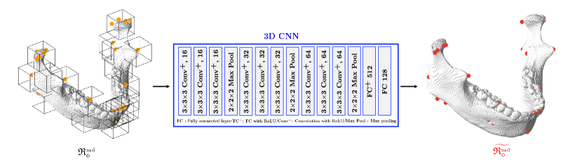
Figure 4: Mandibular landmarks detection. Patch-based 3D CNN is applied to the segmented image of the mandible (separated from the maxilla), in order to capture 3D morphological features of mandible associated with the landmarks. For six landmarks on condyle, we detect them all at once, instead of one by one, because they are positionally related to each other.

For landmarks on the mandible being articulated to the skull, a patch-based 3D CNN is applied to capture the morphological variability of the 3D mandibular surface geometry associated with the landmarks. Let $\mathfrak{R}_{\diamond}^{j}\in\mathbb{R}^{3}$ be a roughly estimated position of a landmark with index $j$ in $\mathfrak{R}_{\diamond}$. See A for details of the landmark index. For each mandibular landmark (i.e., $j\in\{49,\cdots,90\}$), we extract a 3D image patch $(\boldsymbol{x}_{b}^{\mbox{\tiny md}})_{(\eta,\mathfrak{R}_{\diamond}^{j})}$, which is defined by a cube whose edge length is $\eta$ and center is $\mathfrak{R}_{\diamond}^{j}$. By using 3D CNN, we obtain a map $f^{\mbox{\tiny md}}_{j}:(\boldsymbol{x}_{b}^{\mbox{\tiny md}})_{(\eta,\mathfrak{R}_{\diamond}^{j})}\mapsto\widetilde{\mathfrak{R}_{\diamond}}^{j}$, where $\widetilde{\mathfrak{R}_{\diamond}}^{j}$ is an accurate positional estimation for the landmark with index $j$ (i.e., $\widetilde{\mathfrak{R}_{\diamond}}^{j}\approx\mathfrak{R}^{j}$).

To learn the fine detection map $f^{\mbox{\tiny md}}_{j}$, we generate a training dataset by using the paired dataset $\{((\boldsymbol{x}_{b}^{\mbox{\tiny md}})^{(i)},\mathfrak{R}^{(i)})\}_{i=1}^{N_{p}}$ as follows. For a given index $j$, 3D patches with edge lengths of $\eta$ are extracted from $(\boldsymbol{x}_{b}^{\mbox{\tiny md}})^{(i)}$ by varying the center location of patch in basis of label landmark position $(\mathfrak{R}^{(i)})^{j}$. As a result, the following dataset is obtained.

$$\{((\boldsymbol{x}_{b}^{\mbox{\tiny md}})_{(\eta,(\mathfrak{R}^{(i)})^{j}+\textbf{k})}^{(i)},(\mathfrak{R}^{(i)})^{j}):k_{1},k_{2},k_{3}=-\gamma,\cdots,\gamma\mbox{ and }i=1,\cdots,N_{p}\}$$ (11)

where $\textbf{k}\in\mathbb{R}^{3}=(k_{1},k_{2},k_{3})$ and $\eta$ is the maximum length of the center position variation. Using this dataset, the 3D CNN is trained as follows:

$$f^{\mbox{\tiny md}}_{j}=\underset{f^{\mbox{\tiny md}}_{j}\in\mathbb{C}\mathbb{N}\mathbb{N}}{\mbox{argmin}}~{}~{}\sum_{k_{1},k_{2},k_{3}=-\gamma}^{\gamma}\sum_{i=1}^{N_{p}}~{}\|f((\boldsymbol{x}_{b}^{\mbox{\tiny md}})_{(\eta,(\mathfrak{R}^{(i)})^{j}+\textbf{k})}^{(i)})-(\mathfrak{R}^{(i)})^{j}\|_{2}^{2}$$ (12)

where $\mathbb{C}\mathbb{N}\mathbb{N}$ is a class of functions in the form of a 3D CNN. As seen in Figure 4, the 3D CNN is used that possesses an architecture modified from VGGNet [Simonyan2014].

In practice, several landmarks are identified in a group at once. We simultaneously identify six landmarks on the condyle (COR, MCP, LCP, Cp, Ct-in, and Ct-out), which are positionally related to one another, as well as landmarks with bilaterality (e.g. left/right mandibular foramen), which are associated with the symmetric structure of the mandible. For this group detection, we construct a 3D CNN to produce a concatenated vector of all landmark positions on the same group from one 3D image patch.

2.3.2 Detection of cranial landmarks

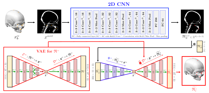
Figure 5: 3D cranial landmark detection using VAE-based low dimensional representation combined with easy-to-find landmarks. Here, the entire cranial landmarks $\mathfrak{R}^{\mbox{\tiny cr}}$ are estimated directly from the knowledge of the reference landmarks $\mathfrak{R}^{\mbox{\tiny cr}}_{\sharp}$ and three landmarks $\mathfrak{R}_{\sharp}^{\mbox{\tiny mid}}$ on midsagittal plane that are obtained by 2D CNN.

Landmarks on the cranium that demonstrates rigidity have less variability between subjects. According to [Yun2020], cranial landmarks have smaller variance compared to mandibular landmarks with the normalization presented in Section 2.1. Moreover, our empirical experiment shown in Figure 6 demonstrates that the rough local-to-global estimation achieved using the VAE-based low dimensional representation provides more accurate annotations for cranial landmarks. Therefore, we again utilize a VAE-based low dimensional representation in the same manner as in Section 2.2 by using only the cranial landmarks $\mathfrak{R}^{\mbox{\tiny cr}}$. To increase the detection accuracy, we enrich the partial knowledge of $\mathfrak{R}^{\mbox{\tiny cr}}$ by accurately detecting three additional cranial landmarks lying near the midsagittal plane (MxDML, Od, and PNS) based on the rough estimation $\mathfrak{R}_{\diamond}$. The overall process is illustrated in Figure 5.

First, we compute a partially integrated image $\boldsymbol{x}^{\mbox{\tiny mid}}$ from $\boldsymbol{x}_{b}^{\mbox{\tiny cr}}$ using (2) so that the center of the truncated volume of $\boldsymbol{x}_{b}^{\mbox{\tiny cr}}$ lies on the midsagittal plane. Next, a 2D patch $(\boldsymbol{x}^{\mbox{\tiny mid}})_{(\eta,\mathfrak{R}_{\diamond}^{j}|_{v_{2},v_{3}})}$ is extracted, which is defined by a square whose edge length is $\eta$ and center is given by $\mathfrak{R}_{\diamond}^{j}|_{v_{2},v_{3}}$. Here, $\mathfrak{R}_{\diamond}^{j}|_{v_{2},v_{3}}$ is a vector eliminating the $v_{1}$ component in the $\mathfrak{R}_{\diamond}^{j}$ and $j\in\{24,25,26\}$. Using a 2D CNN, we learn a function $f^{\mbox{\tiny cr}}_{j}$, which infers an accurate position of a landmark $\mathfrak{R}^{j}$ in $v_{2}$- and $v_{3}$-coordinates ($\mathfrak{R}^{j}|_{v_{2},v_{3}}$) from the 2D image patch $(\boldsymbol{x}^{\mbox{\tiny mid}})_{(\eta,\mathfrak{R}_{\diamond}^{j}|_{v_{2},v_{3}})}$. The landmark position in the $v_{1}$-coordinate is determined by the location of the midsagittal plane.

In the similar manner as in (11), the following training dataset is generated.

$$\small{\{((\boldsymbol{x}^{\mbox{\tiny mid}})_{(\eta,(\mathfrak{R}^{(i)})^{j}|_{v_{2},v_{3}}+\textbf{k})}^{(i)},(\mathfrak{R}^{(i)})^{j}|_{v_{2},v_{3}}):k_{1},k_{2}=-\gamma,\cdots,\gamma\mbox{ and }i=1,\cdot,N_{p}\}}$$ (13)

where $\textbf{k}\in\mathbb{R}^{2}=(k_{1},k_{2})$ and $\eta$ is the maximum length of the center position variation. With the training dataset, the 2D CNN is trained as follows:

$$f^{\mbox{\tiny cr}}_{j}=\underset{f^{\mbox{\tiny cr}}_{j}\in\mathbb{C}\mathbb{N}\mathbb{N}}{\mbox{argmin}}\sum_{k_{1},k_{2}=-\gamma}^{\gamma}\sum_{i=1}^{N_{p}}\|f((\boldsymbol{x}^{\mbox{\tiny mid}})_{(\eta,(\mathfrak{R}^{(i)})^{j}|_{v_{2},v_{3}}+\textbf{k})}^{(i)})-(\mathfrak{R}^{(i)})^{j}|_{v_{2},v_{3}}\|_{2}^{2}$$ (14)

where $\mathbb{C}\mathbb{N}\mathbb{N}$ is a class of functions in the form of a 2D CNN. The architecture of the 2D CNN is modified from VGGNet [Simonyan2014], as illustrated in Figure 4.

Let $\mathfrak{R}_{\sharp}^{\mbox{\tiny mid}}$ be a concatenated positional vector with cranial reference landmarks $\mathfrak{R}^{\mbox{\tiny cr}}_{\sharp}$ and three finely detected landmarks obtained by $f^{\mbox{\tiny cr}}_{j}$. Using this partial knowledge $\mathfrak{R}_{\sharp}^{\mbox{\tiny mid}}$, we find accurate cranial landmark positions $\widetilde{\mathfrak{R}^{\mbox{\tiny cr}}_{\diamond}}$ via

$$\widetilde{\mathfrak{R}^{\mbox{\tiny cr}}_{\diamond}}={\mathcal{D}}^{\mbox{\tiny cr}}\circ\Phi^{\mbox{\tiny cr}}(\mathfrak{R}_{\sharp}^{\mbox{\tiny mid}})$$ (15)

where $\Phi^{\mbox{\tiny cr}}:\mathfrak{R}_{\sharp}^{\mbox{\tiny mid}}\mapsto\textbf{z}^{\mbox{\tiny cr}}$ is a nonlinear map and ${\mathcal{D}}^{\mbox{\tiny cr}}:\textbf{z}^{\mbox{\tiny cr}}\mapsto\mathfrak{R}^{\mbox{\tiny cr}}$ is a decoder of VAE. Here, $\textbf{z}^{\mbox{\tiny cr}}\in\mathbb{R}^{d^{\mbox{\tiny cr}}}$ is a $d^{\mbox{\tiny cr}}$-dimensional latent variable given by $\textbf{z}^{\mbox{\tiny cr}}={\mathcal{E}}(\mathfrak{R}^{\mbox{\tiny cr}})$ and ${\mathcal{E}}^{\mbox{\tiny cr}}:\mathfrak{R}^{\mbox{\tiny cr}}\mapsto\textbf{z}^{\mbox{\tiny cr}}$ is an encoder of VAE. The maps $({\mathcal{E}}^{\mbox{\tiny cr}},{\mathcal{D}}^{\mbox{\tiny cr}})$ and $\Phi^{\mbox{\tiny cr}}$ are trained in the same method presented in (5) and (10) using cranial landmarks $\mathfrak{R}^{\mbox{\tiny cr}}$. The detailed architectures of $({\mathcal{E}}^{\mbox{\tiny cr}},{\mathcal{D}}^{\mbox{\tiny cr}})$ and $\Phi^{\mbox{\tiny cr}}$ are illustrated in Figure 5.

3 Results

3.1 Dataset and experimental settings

Our experiment used a dataset containing 24 paired data (multi-detector CT images and landmark data) and 229 anonymized landmark data. This dataset was provided by Yonsei University, Seoul, Korea. The paired dataset was obtained from normal Korean adult volunteers (9 males and 15 females; 24.22$\pm$2.91 years old) with skeletal class I occlusion and was approved by the local ethics committee of the Dental College Hospital, Yonsei University (IRB number: 2-2009-0026). All informed consents were obtained from each subject. Among 24 paired data, we used 15 data pairs for training (i.e., $N_{p}=15$) and 9 data pairs for testing. The anonymized landmark dataset with 3D landmark coordinates was acquired in an excel format from 229 anonymized subjects with dentofacial deformities and malocclusions (i.e., $N_{l}=229$). Manual landmarking for both dataset was performed by one of the authors (S.-H. Lee) who is an expert in 3D cephalometry with more than 20 years of experience.

Our deep learning method was implemented with Pytorch [Paszke2019] in a computer system with 4 GPUs (GeForce RTX 1080 Ti), two Intel(R) Xeon(R) CPU E5-2630 v4, and 128GB DDR4 RAM. In the training process, the Adam optimizer [Kingma2014] was consistently adopted, which is known as an effective adaptive gradient descent method. In our experiment, all learning parameters (epoch and learning rate) were empirically selected as optimal values via $k$-fold cross validation process [Goodfellow2016].

3.2 Experimental results

3.2.1 Results of reference landmark detection

The detection of the 10 reference landmarks ($\mathfrak{R}_{\#}$) provided very accurate and robust results (see Table 1 and Figure 8). These results almost meet clinical requirements, while the intra-observer repeatability is with a precision less than 1 mm and the overall median inter-observer precision is approximately 2 mm in the 3D landmarking system [Pittayapat2016].

By using reference landmarks, we normalized the landmark data via uniform scaling by fixing the cranial volume of each subject as the average value of the cranial volume for the training dataset.

Landmark	ANS	Bregma	CFM	Or (L)	Po (L)
Mean$\pm$SD(mm)	1.2 $\pm$ 0.45	1.9 $\pm$ 0.53	2.32 $\pm$ 0.88	1.6 $\pm$ 0.335	2.21 $\pm$ 0.87
Landmark	Na	Or (R)	Po (R)	ML (L)	ML (R)
Mean$\pm$SD(mm)	1.73 $\pm$ 0.565	1.3 $\pm$ 0.38	1.63 $\pm$ 1.045	1.96 $\pm$ 0.65	1.72 $\pm$ 0.77

Table 1: Detection error evaluation of 10 reference landmarks. Most of the landmarks are annotated almost within clinical requirements.

3.2.2 Results of the initial local-to-global detection

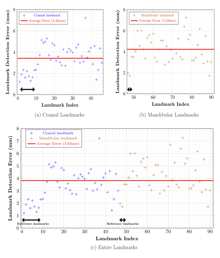
Figure 6: Localization errors (mm) of roughly estimated 90 cephalometric landmarks for the 9 test data using VAE. Blue dots denote the 3D distance error for cranial landmarks, and brown dots represent the 3D distance error for mandibular landmarks. Red line in each diagram represents the average point-to-point error for landmarks included in the diagram.

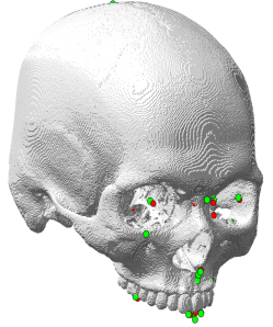
(a) Cranial Landmarks

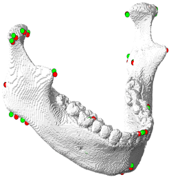
(b) Mandibular Landmarks

Figure 7: Qualitative evaluation of detection for (a) cranial landmarks and (b) mandibular landmarks. The red and green dots denote the ground truth and detected output landmarks respectively.

To conduct the initial local-to-global estimation explained in Section 2.2, 9-dimensional representation was used (i.e., $d=9$ and $\textbf{z}\in\mathbb{R}^{9}$). The VAE $({\mathcal{E}},{\mathcal{D}})$ was trained using 45000 epochs, a full batch-size, and a $0.001$ learning rate. The nonlinear map $\Phi$ was trained with 11000 epochs, a full batch-size, and a $0.0001$ learning rate.

For each landmark, Figure 6 shows the performance evaluation achieved using 9 test data with respect to the averaged 3D point-to-point error. The mean detection error was 3.42 mm for the cranial landmarks (Figure 6(a)), 4.23 mm for the mandibular landmarks (Figure 6(b)), and 3.82 mm for all landmarks (Figure 6(c)). The error of the cranial landmark estimation was much smaller than that of the mandibular landmark estimation.

3.2.3 Result for coarse-to-fine detection

Mandibular landmark detection

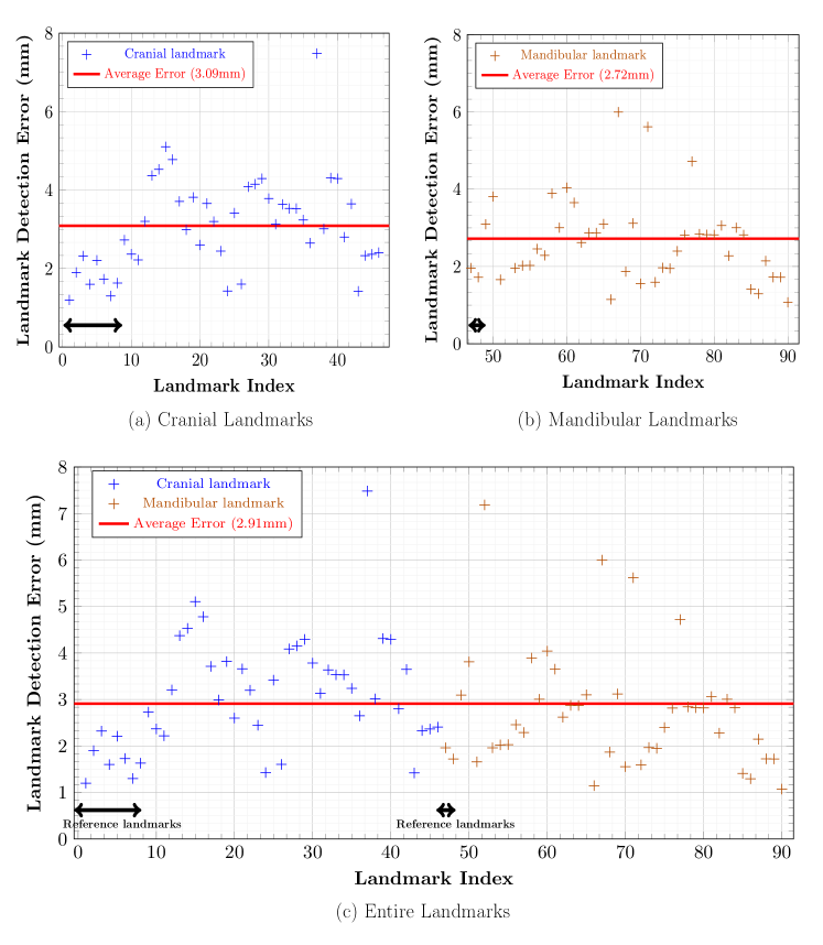
Figure 8: Final localization errors (mm) of 90 cephalometric landmarks for the 9 test data. Blue dots denote the 3D distance error for cranial landmarks, and brown dots represent the 3D distance error for mandibular landmarks. Red line in each diagram represents the average point-to-point error for landmarks included in the diagram.

For fine detection of the mandibular landmarks, 3D image patches were extracted with size of $80\times 80\times 80$ voxels ($\approx 4\times 4\times 4{\mbox{ cm}}^{3}$). To generate the training data in (11), the center location of patch was varied to cover 2 times the maximum error of the initial estimation of $\mathfrak{R}_{\diamond}$ for the training data. Using the parameters of 20000 epochs, a full batch size, and a 0.0001 learning rate, nine 3D CNNs were trained.

Figures 7(b) and 8(b) show the qualitative and quantitative results of the 3D CNNs. The mean 3D distance error decreased to 2.72 mm when compared to the initial detection error of 4.23 mm (Figure 6(b)). According to results shown in Table 3, the proposed method achieved an error range of 1 to 4 mm for the detection of most landmarks. In addition, as shown in Figure 10(b), the proposed method significantly reduced the mean and variance of error for the test subjects, compared to the initial detection.

Cranial landmark detection

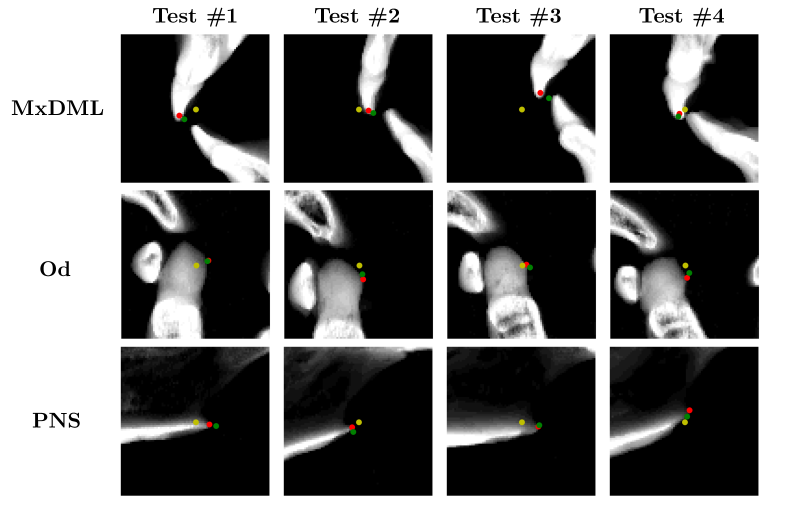
Figure 9: Results of coarse-to-fine landmark detection on 2D patch. Yellow dot is the output of coarsely detected VAE output. Green dot is the output of detection using patch-based CNN. Red dot is the ground truth.

Landmark name	Initial error	2D CNN error	Difference (mm)
MxDML	2.76	1.42	-1.34
Od	4.24	3.41	-0.83
PNS	2.71	1.60	-1.11

Table 2: Error evaluation of the landmarks on the midsagittal plane. Initial error and 2D CNN error are presented in the table. It shows that the errors are reduced after applying 2D CNN.

Error (mm)	1 - 2	2 - 3	3 - 4	4 - 5	5 - 6	6 -	Total
Cranium	7	10	12	14	2	1	46
Mandible	3	2	16	8	10	5	44
Total	10	12	28	22	12	6	90

(a) Initial Estimation

Error (mm)	1 - 2	2 - 3	3 - 4	4 - 5	5 - 6	6 -	Total
Cranium	9	13	14	8	1	1	46
Mandible	15	15	9	2	2	1	44
Total	24	28	23	10	3	2	90

(b) Final Estimation

Table 3: Error tables show the number of landmarks on cranium and mandible that belong to each error range for initial estimation and final estimation.

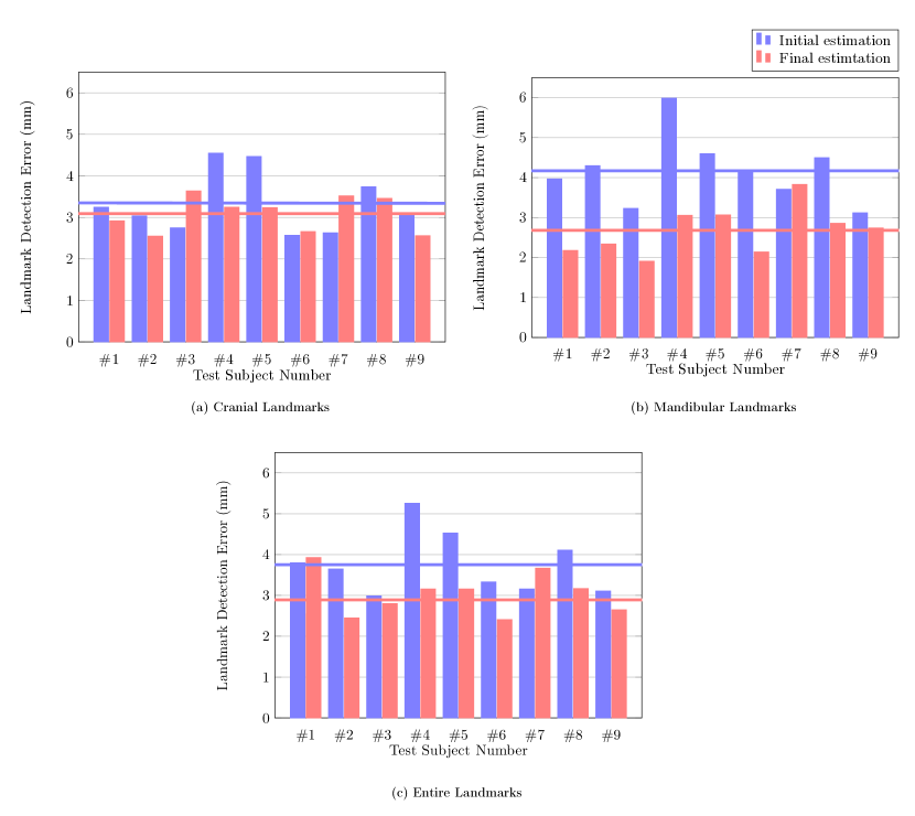
Figure 10: Bar graphs show average point-to-point error of cranial, mandibular and entire landmarks for each of the 9 test data. Blue bars represent the error from the initial estimation, red bars represent the error from the final estimation, and the lines represent average error for all the test data.

To generate the partially integrated image $\boldsymbol{x}^{\mbox{\tiny mid}}$, we set the interval for the truncated volume as $\pm$ 7.5 mm $v_{1}$-directionally from the midsagittal plane. Next, 2D image patches were cropped into sizes of $80\times 80$ pixels ($\approx 4\times 4{\mbox{ cm}}^{2}$). For training the 2D CNNs, we used the learning parameters of 20000 epochs, a full batch-size, and a 0.0001 learning rate.

In Figure 9 and Table 2, qualitative and quantitative evaluations of the 2D CNN-based detection of three cranial landmarks on the midsagittal plane are provided. The detection achieved relatively accurate annotation on the three target landmarks.

For the estimation of all cranial landmarks, VAE $({\mathcal{E}}^{\mbox{\tiny cr}},{\mathcal{D}}^{\mbox{\tiny cr}})$ was trained with 80000 epochs, a full batch, and a $0.001$ learning rate. The map $\Phi^{\mbox{\tiny cr}}$ was trained with 17000 epochs, a full batch-size, and a $0.0001$ learning rate. The latent dimension was set as 15 (i.e., $d^{\mbox{\tiny cr}}=15$, $z^{\mbox{\tiny cr}}\in\mathbb{R}^{15}$).

Figures 7(a) and 8(a) show the final cranial landmark estimation results in qualitative and quantitative formats. The mean detection error for all cranial landmarks was 3.09 mm, which decreased from the initial estimation error of 3.68 mm (Figure 6(a)). As shown in Table 3, the error for most cranial landmarks fell within the range of 1 to 4 mm.

Considering all landmarks, our proposed method achieved an error of 2.91 mm (Figure 8(c)), which is much lower than the initial detection error of 3.82 mm (Figure 6(c)).

4 Discussion

The proposed method employed coarse-to-fine detection, where appropriate strategies for mandibular and cranial landmarks were considered for their different properties. The experiments confirmed the good performance of the proposed method, even when the size of the training dataset is limited. As the amount of training data increases, we expect the detection accuracy to be further improved.

The human skull morphology follows certain patterns and the positions of landmarks are closely interrelated. To learn a low dimensional representation that is strongly associated with the factors determining skull morphology, the proposed method adopted VAE. In our empirical experiment, as shown in Figures 6(a) and 6(b), the VAE-based approach provided more accurate results for the cranial landmark detection due to the rigid property of the cranium compared to the mandible, which has large shape variance. Among the cranial landmarks, the positional estimation of the SC obtained from the relation learned via VAE exhibited the lowest accuracy (see Figure 8). This appears to have occurred because the summit position of the cranium (SC) may weakly depend on the positions of other landmarks. A rigorous factor analysis using VAE may be provided in future research.

Recently, as concerns about the radiation doses have increased, there have been attempts to use dental cone-beam CT for cephalometric analysis instead of the conventional multi-detector CT because cone-beam CT utilizes a much lower radiation dose than multi-detector CT. The investigation of an automated 3D landmarking system for cone-beam CT will therefore be a topic of our future research.

5 Conclusion

This paper proposes a fully automatic landmarking system for 3D cephalometry in 3D CT. The proposed method provides the accurate and reliable identification of cephalometric landmarks that can be used in subsequent clinical studies, such as in the development of morphometrical guidelines for diagnosis, surgical planning, and the treatment of craniofacial diseases. The proposed semi-supervised method is designed to use many anonymized landmark dataset to address the severe shortage of training CT data. Currently, only 24 CT data pairs are available due to legal and ethical restrictions on medical data, while approximately 200 anonymized landmark data are available.

The proposed method has the potential to alleviate experts’ hectic workflow by introducing an automated cephalometric landmarking with high accuracy. In clinical practice, our method allows all 3D landmarks to be estimated from partial information obtained via 3D CT data. Although the error level of some landmarks does not meet the requirement of clinical applications (less than 2 mm), the proposed method may still aid in decisions of clinicians in determining landmark positions, thereby improving their working processes.

Appendix A About 90 cephaometric landmarks

Table 4: Entire 90 cephalometric landmarks and their index.

Location	Index	Landmark	Description
cranium	1	ANS	Anterior nasal spine (reference)
cranium	2	Bregma	Bregma (reference)
cranium	3	CFM	Center of foramen magnum (reference)
cranium	4	Or (L)	Left orbitale (reference)
cranium	5	Po (L)	Left porion (reference)
cranium	6	Na	Nasion (reference)
cranium	7	Or (R)	Right orbitale (reference)
cranium	8	Po (R)	Right porion (reference)
cranium	9	$\sharp$16 tip	The mesiobuccal cusp tip of maxillary right first molar
cranium	10	$\sharp$26 tip	The mesiobuccal cusp tip of maxillary left first molar
cranium	11	ANS’	Constructed ANS point
cranium	12	AO	Anterior occlusal point
cranium	13	FC	Falx cerebri
cranium	14	Clp (L)	Left posterior clinoid process
cranium	15	EC (L)	Left eyeball center
cranium	16	FM (L)	Left frontomaxillary suture
cranium	17	Hyp (L)	Left hypomochlion
cranium	18	M (L)	Left junction of nasofrontal, maxillofrontal, and maxillonasal sutures
cranium	19	NP (L)	Left nasopalatine foramen
cranium	20	Pti (L)	Left inferior pterygoid point
cranium	21	Pts (L)	Left superior pterygoid point
cranium	22	U1 apex (L)	Left upper incisal apex
cranium	23	U1 tip (L)	Left upper incisal tip
cranium	24	MxDML	Maxillary dental midline
cranium	25	Od	Odontoid process
cranium	26	PNS	Posterior nasal spine
cranium	27	Clp (R)	Right posterior clinoid process
cranium	28	EC (R)	Right eyeball center
cranium	29	FM (R)	Right frontomaxillary suture
cranium	30	Hyp (R)	Right hypomochlion
cranium	31	M (R)	Right junction of nasofrontal, maxillofrontal, and maxillonasal sutures
cranium	32	Np (R)	Right nasopalatine foramen
cranium	33	Pti (R)	Right inferior pterygoid point
cranium	34	Pts (R)	Right superior pterygoid point
cranium	35	U1 apex (R)	Right upper incisal apex
cranium	36	U1 tip (R)	Right upper incisal tip
cranium	37	SC	Summit of cranium
cranium	38	mid-Clp	Midpoint between right and left posterior clinoid point
cranium	39	mid-EC	Midpoint between EC (L) and EC (R)
cranium	40	mid-FM	Midpoint between FM (L) and FM (R)
cranium	41	mid-M	Midpoint between M (L) and M (R)
cranium	42	mid-Np	Midpoint between Np (L) and Np (R)
cranium	43	mid-Or	Midpoint between Or (L) and Or (R)
cranium	44	mid-Po	Midpoint between Po (L) and Po (R)
cranium	45	mid-Pti	Midpoint between Pti (L) and Pti (R)
cranium	46	mid-U1 tip	Midpoint between U1 tip (L) and U1 tip (R)
mandible	47	MF (L)	Left mental foramen (reference)
mandible	48	MF (R)	Right mental foramen (reference)
mandible	49	$\sharp$36 tip	The mesiobuccal cusp tip of mandibular left first molar
mandible	50	$\sharp$46 tip	The mesiobuccal cusp tip of mandibular right first molar
mandible	51	CON (L)	Left condylar point
mandible	52	COR (L)	Left coronoid point
mandible	53	Cp (L)	Left posterior condylar point
mandible	54	Ct-in (L)	Left medial temporal condylar point
mandible	55	Ct-mid (L)	Midpoint between left Ct-in and Ct-out
mandible	56	Ct-out (L)	Left lateral temporal condylar point
mandible	57	F (L)	Left mandibular foramen
mandible	58	Go-in (L)	Left inferior gonion point
mandible	59	Go-mid (L)	Midpoint between left posterior and inferior gonion point
mandible	60	Go-post (L)	Left posterior gonion point
mandible	61	L1 apex (L)	Root apex of left mandibular central incisor
mandible	62	L1 tip (L)	Incial tip midpoint of left mandibular central incisor
mandible	63	LCP (L)	Left lateral condylar point
mandible	64	MCP (L)	Left medial condylar point
mandible	65	a-Go notch (L)	Left antegonial notch
mandible	66	mid-F MF (L)	Midpoint between left mandibular foramen and mental foramen
mandible	67	Me (anat)	Anatomical menton
mandible	68	MnDML	Mandibular dental midline
mandible	69	Pog	Pogonion
mandible	70	CON (R)	Right condylar point
mandible	71	COR (R)	Right coronoid point
mandible	72	Cp (R)	Right posterior condylar point
mandible	73	Ct-in (R)	Right medial temporal condylar point
mandible	74	Ct-mid (R)	Midpoint between right Ct-in and Ct-out
mandible	75	Ct-out (R)	Right lateral temporal condylar point
mandible	76	F (R)	Right mandibular foramen
mandible	77	Go-in (R)	Right inferior gonion point
mandible	78	Go-mid (R)	Midpoint between right posterior and inferior gonion point
mandible	79	Go-post (R)	Right posterior gonion point
mandible	80	L1 apex (R)	Root apex of right mandibular central incisor
mandible	81	L1 tip (R)	Incial tip midpoint of right mandibular central incisor
mandible	82	LCP (R)	Right lateral condylar point
mandible	83	MCP (R)	Right medial condylar point
mandible	84	a-Go notch (R)	Right antegonial notch
mandible	85	mid-F MF (R)	Midpoint between right mandibular foramen and mental foramen
mandible	86	mid-Cp	Midpoint between right and left posterior condylar point
mandible	87	mid-F	Midpoint between F (L) and F (R)
mandible	88	mid-L1 tip	Midpoint between L1 tip (L) and L1 tip (R)
mandible	89	mid-MF	Midpoint between MF (L) and MF (R)
mandible	90	midpoint of mid-F MF (R/L)	Midpoint between mid-F MF (R) and mid-F MF (L)

References

- \harvarditemAdams et al 2004Adams2004 G. L. Adams, S. A. Gansky, A. J. Miller, W. E. Harrell Jr, and D. C. Hatcher 2004 Comparison between traditional 2-dimensional cephalometry and a 3-dimensional approach on human dry skulls American journal of orthodontics and dentofacial orthopedics 126(4) 397-409
- [1] \harvarditemArik et al 2017Arik2017 S.. Arik, B. Ibragimov and L. Xing 2017 Fully automated quantitative cephalometry using convolutional neural networks J Med Imaging (Bellingham) 4(1) 014501
- [2] \harvarditemCodari et al 2017Codari2017 M. Codari, M. Caffini, G.M. Tartaglia, C. Sforza, and G. Baselli 2017 Computer-aided cephalometric landmark annotation for CBCT data International journal of computer assisted radiology and surgery 12(1) 113-121
- [3] \harvarditemKang et al 2020Kang2020 S. H.Kang, K. Jeon, H. Kim, J.K. Seo, and S. Lee 2020 Automatic three-dimensional cephalometric annotation system using three-dimensional convolutional neural networks: a developmental trial Computer Methods in Biomechanics and Biomedical Engineering: Imaging & Visualization 8(2) 210-218
- [4] \harvarditemKingma et al 2013Kingma2013 D. P. Kingma, M. Welling, 2013 Auto-encoding variational bayes. arXiv preprint arXiv:1312.6114
- [5] \harvarditemKingma et al 2014Kingma2014 D. P. Kingma, J. Ba, 2014 Adam: A method for stochastic optimization arXiv preprint arXiv:1412.6980
- [6] \harvarditemLee et al 2014Lee2014 S.-H. Lee, T.-J. Kil, K.-R. Park, B.C. Kim, Z. Piao, and P. Corre 2014 Three-dimensional architectural and structural analysis-a transition in concept and design from Delaire’s cephalometric analysis Int J Oral Maxillofac Surg 43 1154-1160
- [7] \harvarditemLee et al 2019Lee2019 S. M. Lee, H. P. Kim, K. Jeon, S. H. Lee and J. K. Seo 2019 Automatic 3D cephalometric annotation system using shadowed 2D image-based machine learning Physics in medicine and biology 64(5) 055002
- [8] \harvarditemMontufar et al 2018Montufar2018 J. Montufar, M. Romero, and R. J. Scougall-Vilchis 2018 Automatic 3-dimensional cephalometric landmarking based on active shape models in related projections American Journal of Orthodontics and Dentofacial Orthopedics 153(3) 449-458
- [9] \harvarditemNalcaci et al 2010Nalcaci2010 R. Nalçaci, F. Öztürk, and O. Sökücü 2010 A comparison of two-dimensional radiography and three-dimensional computed tomography in angular cephalometric measurements. Dentomaxillofacial Radiology 39(2) 100-106
- [10] \harvarditemTenti1981Tenti1981 F. Tenti 1981 Cephalometric analysis as a tool for treatment planning and evaluation The European Jornal of Orthodontics 3(4) 241-245
- [11] \harvarditemProffit et al 2018Proffit2018 W. Proffit, H. Fields, B. Larson and D.Sarver 2018 Contemporary Orthodontics Vol. 6th Edition, Mosby
- [12] \harvarditemPittayapat et al 2014Pittayapat2014 P. Pittayapat, N. Limchaichana-Bolstad, G. Willems and R. Jacobs 2014 Three-dimensional cephalometric anlaysis in orthodontics: a systematic review Orthodontics & craniofacial research 17(2) 69-91
- [13] \harvarditemLindner et al 2016Lindner2016 C. Lindner, C.-W. Wang, C.-T. Huang, C.-H. Li, S.-W. Chang and T. F. Cootes 2016 Fully automatic system for accurate localisation and analysis of cephalometric landmarks in lateral cephalograms Scientific reports 6 33581
- [14] \harvarditemYun et al 2020Yun2020 H. S. Yun, T.J. Jang, S. M. Led and J.K. Seo Learning-based local-to-global landmark annotation for automatic 3d cephalometry Physics in Medicine & Biology 65(8) 085018
- [15] \harvarditemVallabh et al 2019Vallabh2019 R. Vallabh, J. Zhang, J. Fernandez, G.Dimitroulis and D. C. Ackland 2019 The morphology of the human mandible: A computational modelling study Biomechanics and Modeling in Mechanobiology 1-16
- [16] \harvarditemJang et al 2020Jang2020 T. J. Jang, K. C. Kim, H. C. Cho and J. K. Seo 2020 A fully automated method for 3d individual tooth identification and segmentation in dental cbct arXiv
- [17] \harvarditemSimonyan et al 2014Simonyan2014 K. Simonyan and A. Zisserman 2014 Very deep convolutional networks for large-scale image recognition arXiv
- [18] \harvarditemPaszke et al 2019Paszke2019 A. Paszke, S. Gross, F. Massa, A. Lerer, J. Bradbury , G. Chanan, T. Killeen, Z. Lin, N. Gimelshein, L. Antiga, et al. 2019 Pytorch: An imperative style, high-performance deep learning library Advances in neural information processing systems 8026-2037
- [19] \harvarditemGoodfellow et al 2016Goodfellow2016 I. Goodfellow, Y. Bengio and A. Courville 2016 Deep Learning MIT Press
- [20] \harvarditemPittayapat et al 2016Pittayapat2016 P. Pittayapat, R. Jacobs, M. M. Bornstein, G. A. Odri, M. S. Kwon, I. Lambrichts, G. Willems, C. Politis and R. Olszewski 2016 A new mandible-specific landmark reference system for three-dimensional cephalometry using cone-beam computed tomography European journal of orthodontics 38(6) 563-568
- [21]