Accurate Camouflaged Object Detection via Mixture Convolution and Interactive Fusion

Abstract

Camouflaged object detection (COD), which aims to identify the objects that conceal themselves into the surroundings, has recently drawn increasing research efforts in the field of computer vision. In practice, the success of deep learning based COD is mainly determined by two key factors, including (i) A significantly large receptive field, which provides rich context information, and (ii) An effective fusion strategy, which aggregates the rich multi-level features for accurate COD. Motivated by these observations, in this paper, we propose a novel deep learning based COD approach, which integrates the large receptive field and effective feature fusion into a unified framework. Specifically, we first extract multi-level features from a backbone network. The resulting features are then fed to the proposed dual-branch mixture convolution modules, each of which utilizes multiple asymmetric convolutional layers and two dilated convolutional layers to extract rich context features from a large receptive field. Finally, we fuse the features using specially-designed multi-level interactive fusion modules, each of which employs an attention mechanism along with feature interaction for effective feature fusion. Our method detects camouflaged objects with an effective fusion strategy, which aggregates the rich context information from a large receptive field. All of these designs meet the requirements of COD well, allowing the accurate detection of camouflaged objects. Extensive experiments on widely-used benchmark datasets demonstrate that our method is capable of accurately detecting camouflaged objects and outperforms the state-of-the-art methods.

1 Introduction

Camouflage is a biological phenomenon widely existing in nature. Biologists have found that creatures in nature often conceal themselves from predators using their own structures and physiological characteristics. For instance, a chameleon can change the color of its body when the environment changes; A crab usually finds the habitat that is similar to its appearance; etc. These animals camouflage themselves for the survival purpose, such as avoiding being attacked, communication, and courtship. The earliest research of camouflage can be traced back to the last century. Thayer et al. [1] systematically studied the phenomenon of camouflage in 1918. A hundred years have passed, and biologists keep the passion in studying this significant natural phenomenon.

Due to its important scientific and practical value [2], significant efforts have been made to detect/segment the camouflaged objects from natural scenes, which raises the demands of effective camouflaged object detection (COD) approaches. However, compared with the traditional object detection/segmentation tasks [3, 4] in computer vision, COD shows considerable difficulties due to the low boundary contrast between the camouflaged object and its surroundings. To address this challenge, a number of methods have been proposed to accurately detect/segment camouflaged objects (see Fig. 1 for a brief timeline of COD). For instance, Zhang et al. [5] proposed a Bayesian approach to detect moving camouflaged objects. Deep learning has shown remarkable success in COD and a number of deep-based COD methods have been proposed. Le et al. [6] designed a general end-to-end network, called anabranch network, for camouflaged object segmentation. Fan et al. [2] presented a large COD dataset, called COD10K, and a new COD model, called SINet, which promotes the COD research to a new level.

\begin{overpic}[width=433.62pt]{Imgs/timeline1.pdf} \par\end{overpic}

Figure 1: A brief timeline of camouflaged object detection. The definition of camouflage in animal can be traced back to CCAK [1]. The first deep learning based COD approach is HAD [7] proposed in 2017. Recently, Fan et al. [2] proposes the largest COD dataset COD10K, which greatly promotes the development of COD.

Despite their advantages, existing deep-based COD methods suffer from two major limitations. First, they usually overlook the importance of large receptive field. In practice, the context information plays an important role in COD, implying that a large receptive is greatly desired since it is able to provide rich context features, which are essential to the accurate detection of camouflaged objects. Second, most methods fuse the multi-scale features using very simple operations, e.g., concatenation and addition, which are unable to capture the valuable information highly-related to the detection of camouflaged objects. This inevitably results in unsatisfactory performance and raises the demands of more advanced feature fusion strategies.

To this end, we propose a novel deep-based COD model, which employs specially-designed mixture convolution and interactive fusion (MCIF) techniques to accurately detect the camouflaged objects from natural scenes. Our method, called MCIF-Net, harnesses an effective attention-based fusion strategy to aggregate the rich context features extracted from a larger receptive field, which well fits the scenario of accurate COD and overcomes the limitations in existing methods. In MCIF-Net, we first extract multi-level features from a backbone network. The resulting features are then fed to our dual-branch mixture convolution (DMC) modules for extracting rich context features from a large receptive field. The DMC module is in a dual-branch form with multiple asymmetric convolutional layers and two dilated convolutional layers, which significantly enlarges the receptive field. Finally, we propose multi-level interactive fusion (MIF) modules to aggregate the rich context features for the accurate detection of camouflaged objects. Our MIF module employs an attention mechanism along with feature interaction, allowing effective feature fusion.

In a nutshell, the contributions of this paper contain threefold:

• We propose a novel feature fusion module, MIF, to effectively aggregates the multi-level features for accurately detecting camouflaged objects. Our MIF module employs an advanced interactive attention mechanism for feature fusion, which guarantees the remarkable performance of MCIF-Net.

• We propose an effective receptive field module, DMC, which utilizes multi-type convolution operations to enlarge the receptive field. Our DMC module provides rich context features for COD, boosting the performance significantly.

• Extensive experiments are performed using COD benchmark datasets. The experimental results demonstrate that our MCIF-Net outperforms existing cutting-edge models and advances the state-of-the-art performance. In addition, our ablation studies sufficiently demonstrate the effectiveness of two proposed modules, i.e., MIF and DMC.

Our paper is organized as follows. In Section 2, we discuss a number of works that are closely related to ours. In Section 3, we provide detailed descriptions for our MCIF-Net and the associated modules. In Section 4, we present the implementation details, datasets, evaluation metrics, and experimental results. Finally, we conclude this work and present future directions in Section 6.

2 Related Works

2.1 Camouflage

Camouflage has been studied for a long time. A large number of biologists explored the typical instances of camouflage and explained camouflage using the principles of natural selection and adaptation. Inspired by this important natural phenomenon, humans have made attempts to imitate these pattern in many fields, such as art, agriculture, etc. Camouflage also gained attention from the optical researchers [8], who proposed the signature strength metrics for camouflaged objects. Some works have been made to analyze the camouflaged images and to study how to create digital camouflaged images [9]. With the rapid development of information technologies, COD has drawn increasing research efforts from the computer vision community [10]. In particular, Fan et al. [2] performed a comprehensive study on COD from the perspective of computer vision and provided an elaborate datasets, i.e., COD10K, which contains 10,000 pictures of 69 categories. Moreover, efforts have been directed to identifying camouflaged objects using motion information [11] or bio-inspired adversarial attack [12].

2.2 Attention Mechanism

Attention mechanism is inspired by the fact that human beings or understanding scenes are not visual analysis of the whole scene, but significant parts. A number of attention modules have been embedded into the CNN network to improve the understanding ability of the network, which also enables to capture the long-range dependency. For self-attention mechanisms [13], a weighted sum of all positions in spatial temporal domain is calculated as the response at a position. Squeeze-and-excitation network [14] formulates channel-wise relationships via an attention-and-gating mechanism. Spatial and channel-wise attention (SCA) [15] utilizes both channel wise attention and spatial attention for image captioning. Similar to SCA, bottleneck attention module [16] and convolutional block attention module [17] infer attention maps along two separated dimensions, i.e., channel and spatial, and employs multiple attention maps for adaptive feature refinement. Fu et al. [18] constructed a novel self-attention network consisted of two parallel attention modules, including a position attention module used to obtain the dependency of any two positions in the feature map, and a channel attention module for the dependency between any two channels. Different from existing attention mechanisms, we propose the MIF module based on an interactive attention mechanism, allowing the effective fusion of multi-level features.

2.3 Receptive Field Module

A number of methods have been proposed to study the receptive field in CNN. Typical instances include the inception block [19], spatial pyramid pooling (SPP) [20], atrous spatial pyramid pooling (ASPP) [21], and receptive field block (RFB) [22]. Inception block [19] consists of multiple branches, where the standard convolutional layers with different kernel sizes are employed to extract multi-level features. The resulting features are then combined as the output, which encodes the rich representations from a large receptive filed. However, inception block may loss some crucial details since all the kernels are used at the same center. Different from the inception block, SPP [20] generates a fixed-length feature vector from the feature maps with different scales, and transmitted it to the fully connected layer through pooling of three scales. ASPP [21] introduces dilated convolution for enlarged receptive field, however it uses same kernel size, which may lead to a confusion between context and object. To resolve these limitations, RFB [22] assigns larger weights to the positions nearer to the center, providing improved performance.

\begin{overpic}[width=424.94574pt]{Imgs/network_new.pdf} \end{overpic}

Figure 2: An overview of our MCIF-Net. Based on the features from backbone, we first utilize multiple dual-branch mixture convolution modules to extract rich context features and then fuse the features with our multi-level interactive fusion modules for the accurate detection of camouflaged object.

3 Method

An overview of our MCIF-Net is shown in Fig. 2. In general, MCIF-Net consists of a ResNet-50 based backbone and two kinds of key modules, i.e., dual-branch mixture convolution (DMC) module and multi-level interactive fusion (MIF) module. In what follows, we will first present the overall architecture of MCIF-Net in Section 3.1. We will then detail in two proposed key modules, i.e., DMC (Section 3.2) and MIF (Section 3.3). Finally, we will describe our loss function in Section 3.4.

3.1 Network Architecture

As shown in Fig. 2, given a RGB image $\mathbf{X}\in{\mathbb{R}^{W\times H\times 3}}$, where $H$ and $W$ denote the image width and height, respectively, we first extract four-scale hierarchical features using a backbone network. However, the resulting features, denoted as $\{\mathbf{X}^{(i)}\}_{i=1}^{4}$, are unable to capture the rich context information since they are limited by a small receptive field.

To resolve this issue, we feed each $\mathbf{X}^{(i)}$ to the corresponding DMC module, which is capable of extracting rich context features from a large receptive field. The resulting rich context features $\mathbf{X}_{\text{d}}^{(i)}$ is computed as

$$\mathbf{X}_{\text{d}}^{(i)}=\mathit{f}_{\text{DMC}}^{(i)}({\mathbf{X}^{(i)}}),$$ (1)

where $f_{\text{DMC}}^{(i)}(\cdot)$ denotes a function acting as the $i$th DMC module.

To explore the correlations between the features from adjacent layers, we multiply them element-wisely, resulting new features $\mathbf{X}^{(j)}_{\text{m}}=\mathbf{X}_{\text{d}}^{(j)}\odot\mathbf{X}_{\text{d}}^{(j+1)}$, where $\odot$ denotes the Hadamard product, i.e., element-wise multiplication, and $j\in\{1,2,3\}$. After that, we employ the attention mechanism to effectively fuse the features at different levels. As shown in Fig. 2, three MIF modules are adopted, where each MIF has two inputs, including multiplication features $\mathbf{X}_{\text{m}}^{(j)}$ and the features from the last MIF, i.e.,

$$\mathbf{X}_{\text{a}}^{(j)}=f_{\text{MIF}}^{(j)}(\mathbf{X}_{\text{m}}^{(j)},\mathbf{X}_{\text{a}}^{(j+1)}),$$ (2)

where $\mathbf{X}_{\text{a}}^{(j)}$ is the output of $j$th MIF module, and $f_{\text{MIF}}^{(j)}(\cdot)$ denotes a function acting as the $j$th MIF module. Note that $\mathbf{X}_{\text{a}}^{(4)}$ denotes the features provided by the fourth DMC module, i.e., $\mathbf{X}_{\text{a}}^{(4)}=\mathbf{X}_{\text{d}}^{(4)}$.

Finally, we feed $\mathbf{X}_{\text{a}}^{(1)}$ to a convolutional layer for the final prediction $P^{(1)}$, which is a map encoding the pixel-wise probabilities of camouflaged objects. Note that we provides supervisions for the predictions given by other two MIF modules and the fourth DMC module, i.e., $P^{(2)}$, $P^{(3)}$, and $P^{(4)}$ during the training.

3.2 Dual-branch Mixture Convolution Module

To enlarge the receptive filed, we propose a novel receptive filed module, DMC, which is a stack of asymmetric convolutional and dilated convolutional layers. As shown in 2, we employ the DMC to extract rich context features on each side output of the backbone network.

Specifically, the DMC $f_{\text{DMC}}^{(i)}(\cdot)$ first utilizes a convolutional layer with $kernel=3\times 3$ to coarsely transform the features $\mathbf{X}^{(i)}$ from the backbone network. To learn equally-spatial-sized features with a significantly larger receptive field, the resulting features are then projected to two independent branches, where each of them is equipped with a convolutional layer with $kernel=1\times 1$ for changing the number of channels, followed by a pair of asymmetric convolutional layers with $kernel=1\times n$ and $kernel=n\times 1$ for enlarging the receptive field, where $n=5$ for the top branch and $n=7$ for the bottom branch. To maximize the co-characterization between two branches, we add the features from two branches for the superimposed features, i.e.,

$$\mathbf{\hat{X}}^{(i)}=\mathbf{X}^{(i)}_{\text{TB}}+\mathbf{X}^{(i)}_{\text{BB}},\\$$ (3)

where $\mathbf{X}^{(i)}_{\text{TB}}$ and $\mathbf{X}^{(i)}_{\text{BB}}$ denote the features from top branch and bottom branch, respectively.

To further enlarge the receptive field, we project features to two branches equipped with the dilated convolutional layers [23] with the same kernel size ($kernel=3\times 3$) and different rates ($rate=5$ for the top branch and $rate=7$ for the bottom branch). Finally, we merge again using the element-wise addition and utilize a convolutional layer with $kernel=3\times 3$ followed by a ReLU activation function [24] for the rich context features $\mathbf{X}_{\text{d}}^{(i)}$, i.e.,

$$\mathbf{X}_{\text{d}}^{(i)}=CR({DC_{r=5}}(\mathbf{\hat{X}}^{(i)})+{DC_{r=7}}(\mathbf{\hat{X}}^{(i)})),$$ (4)

where $DC_{r=5}(\cdot)$ and $DC_{r=7}(\cdot)$ represent the dilated convolutional layers with different rates, $r$, and $CR(\cdot)$ denotes the combination of the final convolutional layer and a ReLU activation function.

\begin{overpic}[width=433.62pt]{Imgs/MIF.pdf} \end{overpic}

Figure 3: Illustration of our multi-level interactive fusion module. We fuse the multi-level features using an interactive attention mechanism.

3.3 Multi-level Interactive Fusion Module

We then fuse the rich context features from DMC modules using our MIF modules. Unlike existing feature fusion strategies, which usually rely on simple feature addition (e.g., EGNet [25]) and concatenation (e.g., UNet++ [26]), our MIF module fuses the multi-level features using an attention mechanism along with feature interaction, allowing effective feature fusion for the accurate detection of camouflaged objects.

Fig. 3 illustrates the architecture of MIF module. Denote the low- and high-level features as $\mathbf{X}_{\text{l}}$ and $\mathbf{X}_{\text{h}}$. We first utilize two symmetric branches to process two levels of features and then employ the features in two branches to enhance each other. Using the low-level branch as an example, we feed $\mathbf{X}_{\text{l}}$ to a convolution block and have new features denoted as $CBR(\mathbf{X}_{\text{l}})$, where $CBR(\cdot)$ denotes a convolution block with a convolutional layer ($kernel=3\times 3$) followed by a batch normalization layer and a ReLU activation function. At each spatial location, we then computed the statistics, i.e., the average and maximum, across the channel dimension. Mathematically, the resulting informative spatial attention maps $M_{\text{l,max}}$ and $M_{\text{l,mean}}$ are defined as

$$M_{\text{l,max}} =\sigma(max_{\text{c}}(CBR(\mathbf{X}_{\text{l}}))),$$ (5)

$$M_{\text{l,mean}} =\sigma(mean_{\text{c}}(CBR(\mathbf{X}_{\text{l}}))),$$ (6)

where $max_{\text{c}}(\cdot)$ and $mean_{\text{c}}(\cdot)$ denote two respective operations for computing max and mean maps across the channel dimension, and $\sigma(\cdot)$ denotes the Sigmoid activation function. Similarly, for the high-level branch, we have $M_{\text{h,max}}$ and $M_{\text{h,mean}}$, which are generated using $\mathbf{X}_{\text{h}}$ with the same procedure.

After that, we enhance the attention maps form two branches. For the low-level branch, the enhancement process is described as follows

$$M_{\text{l,max}}=mul(M_{\text{l,max}},\vartheta(M_{\text{h,mean}})),$$ (7)

$$M_{\text{l,mean}}=mul(M_{\text{l,mean}},\vartheta(M_{\text{h,max}}),$$ (8)

where $mul(\cdot)$ denotes the product operation, $\vartheta(\cdot)$ denotes the resizing operation used to match the dimensions of low- and high-level attention maps. Similarly, for the high-level branch, we compute the enhanced attention maps as

$$M_{\text{h,max}}=mul(M_{\text{h,max}},\vartheta(M_{\text{l,mean}})),$$ (9)

$$M_{\text{h,mean}}=mul(M_{\text{h,mean}},\vartheta(M_{\text{l,max}})).$$ (10)

We then concatenate the attention maps $M_{\text{l,mean}}$ and $M_{\text{l,max}}$ together and then feed the concatenated map to a convolutional layer with $kernel=1\times 1$ so that the resulting attention map $M_{\text{l}}$ is one-channel. We do the same for $M_{\text{h,max}}$ and $M_{\text{h,mean}}$ and have $M_{\text{h}}$. After that, we pass $M_{\text{l}}$ and $M_{\text{h}}$ to two softmax layers $\eta(\cdot)$ and enhance the original features using

$$\mathbf{\hat{X}}_{\text{l}} =mul(\eta(M_{\text{l}}),{\mathbf{X}_{\text{l}}})+{\mathbf{X}_{\text{l}}},$$ (11)

$$\mathbf{\hat{X}}_{\text{h}} =mul(\eta(M_{\text{h}}),{\mathbf{X}_{\text{h}}})+{\mathbf{X}_{\text{h}}}.$$ (12)

Finally, we upsample $\mathbf{\hat{X}}_{\text{l}}$ and feed $\mathbf{\hat{X}}_{\text{h}}$ to a convolutional block so that the resulting low- and high-level features, $\vartheta({\mathbf{\hat{X}}_{\text{l}}})$ and $CBR({\mathbf{\hat{X}}_{\text{h}}})$, share the same dimensions. Finally, we perform element-wise multiplication and feed the features to the last convolutional block for the final enhanced features $\mathbf{X}_{\text{a}}$. Mathematically, $\mathbf{X}_{\text{a}}$ is computed using

$$\mathbf{X}_{\text{a}}={CBR}(mul(\vartheta({\mathbf{\hat{X}}_{\text{l}}}),CBR({\mathbf{\hat{X}}_{\text{h}}}))).$$ (13)

3.4 Loss Function

The binary cross-entropy (BCE) loss is widely used in binary segmentation. However, it is only defined in a shallow pixel level, which leads to unsatisfactory performance when there is imbalanced problem. The intersection-over-union (IoU) loss proposed in BASNet [27] resolves the limitation in BCE by putting more attention on the regional level. Therefore, we combine these two loss functions to design ours. In addition, we notice the category imbalance issue of positive (foreground pixel) and negative (background pixel) samples in the training dataset. To resolve this issue, we add an additional balance parameter for each pixel, termed as $\lambda_{n}$, which is defined as

$$\lambda_{n}=\sigma(|P_{n}-G_{n}|),$$ (14)

where $G_{n}$ and $P_{n}$ are the values at pixel $n$ in our prediction $P$ and the ground-truth label $G$, respectively. We then define the improved BCE loss function $\mathcal{L}_{\text{BCE}}(P,G)$ as

$$\mathcal{L}_{\text{BCE}}(P,G)=-\sum\nolimits_{n=1}^{N}[\lambda_{n}*(G_{n}\log(P_{n})+(1-G_{n})\log(1-P_{n}))],$$ (15)

where $N=H\times W$ is the total number of pixels. In addition, we use IoU loss function $\mathcal{L}_{\text{IoU}}(P,G)$ to focus on regions. The IoU loss is defined as

$$\mathcal{L}_{\text{IoU}}(P,G)=1-\frac{{\sum\nolimits_{n=1}^{N}{[{P_{n}}\times{G_{n}}]}}}{{\sum\nolimits_{n=1}^{N}{[{P_{n}}+{G_{n}}-{P_{n}}\times{G_{n}}]}}},$$ (16)

Finally, we provide supervisions for all three MIF modules and the last DCM module, and define the total loss function $\mathcal{L}$ as

$$\mathcal{L}=\sum_{i=1}^{4}[\mathcal{L}_{\text{BCE}}(P^{(i)},G)+\mathcal{L}_{\text{IoU}}(P^{(i)},G)],$$ (17)

where $i$ indicates the index of predictions, shown in Fig. 2.

4 Experiments

4.1 Implementation Details

The proposed MCIF-Net is implemented using PyTorch and will be made publicly available at https://github.com/BigHeartDB/MCIFNet. We adopt ResNet-50 as our backbone and only keep the feature extraction part, which is initialized by the pre-trained model on ImageNet. We follow [2] to resize the input images to $352\times 352$ during both training and testing. We follow the experimental setting in [2] and utilize the same dataset for training and testing. The network is trained using an SGD optimizer with an initial learning rate of 0.005, weight decay of 0.0005, and momentum of 0.95. The batch size is set to 16. The training takes 55 minutes for 32 epochs and the test speed reaches 37 Fps in a computer equipped with an Intel Xeon E5-2640 CPU (2.6GHz) and a RTX 2080 GPU.

4.2 Datasets

To evaluate our method thoroughly, we perform extensive experiments on on COD benchmark datasets, including CAMO [6] and COD10K [2]. CAMO is the first formal COD dataset, where each image contains more than one camouflaged objects with pixel-level labels. The COD10K is the largest COD dataset with pixel-level annotations, which is composed of four main categories (Amphibian, Acoustic, Flying Territorial) and 69 sub-classes. The Amphibian contains 124 pictures with complex background, which are mainly focused on small targets. The Aquatic contains 474 pictures of camouflaged objects in the water mainly with slender trunks and complex edges. The Flying contains 714 pictures, which are mainly focused on small targets and partially occluded objects. The Terrestrial is composed of 699 pictures, which contains abundant land creatures with small structure and slender limbs.

4.3 Evaluation Criteria

The COD belongs to the task of binary segmentation, therefore we perform quantitative evaluations using a number of popular binary segmentation evaluation criteria, including S-measure [28], E-measure [29], weighted F-measure, and mean absolute error.

S-measure ($S_{\alpha}$). We use S-measure to calculate the spatial structure similarity between the prediction and the ground-truth in the object-aware level $S_{o}$ and the region-aware level $S_{r}$. Mathematically, the S-measure $S_{\alpha}$ is defined as

$$S_{\alpha}=\alpha S_{o}+(1-\alpha)S_{r},$$ (18)

where $\alpha$ is a tuning parameter and is set to $0.5$ according to [28].

E-measure ($E_{\phi}$). As a binary map evaluation metric, E-measure is designed for evaluating the difference between the predicted map $P$ and ground-truth label $G$ from the local and global perspectives. It is defined as

$$E_{\phi}=\frac{1}{W\times H}\sum_{x=1}^{W}\sum_{y=1}^{H}\phi(P(x,y)-G(x,y)),$$ (19)

where $\phi(\cdot)$ denotes the enhanced alignment matrix. Following [2], we report the mean E-measure in the paper.

Weighted F-measure ($F_{\beta}^{w}$). As an improved version of F-measure, $F_{\beta}^{w}$ is defined based on weighted Recall and Precision to avoid the influence of threshold, i.e.,

$$F_{\beta}^{w}=\frac{\left(1+\beta^{2}\right)\text{Precision}^{w}\times\text{Recall}^{w}}{\beta^{2}\times\text{Precision}^{w}+\text{Recall}^{w}},$$ (20)

where $\beta$ is a tuning parameter and is set to 0.3 according to [2].

Mean absolute error (MAE, $M$). We employ MAE to measure the average absolute distance between the normalized predicted map and the ground-truth. Specifically, MAE is defined as

$$M=\frac{1}{W\times H}\sum_{x=1}^{W}\sum_{y=1}^{H}\left|P(x,y)-G(x,y)\right|.$$ (21)

Table 1: Quantitative results on COD benchmark datasets. The best and second best results are marked by red and blue colors, respectively. All methods are trained using the same dataset, as in [2]. $\uparrow$ indicates the higher the score the better, and vice versa for $\downarrow$. We evaluate the results using four widely used metrics, including S-measure ($S_{\alpha}$), E-measure ($E_{\phi}$), F-measure ($F_{\beta}^{w}$), and MAE ($M$). Amp., Aqu., Fly., and Ter. are short names for Amphibian, Aquatic, Flying, and Terrestrial, respectively.

	Model	Amp. (COD10K [2])				Aqu. (COD10K [2])				Fly. (COD10K [2])				Ter. (COD10K [2])				CAMO [6]
		$S_{\alpha}\uparrow$	$E_{\phi}\uparrow$	$F_{\beta}^{w}\uparrow$	$M\downarrow$	$S_{\alpha}\uparrow$	$E_{\phi}\uparrow$	$F_{\beta}^{w}\uparrow$	$M\downarrow$	$S_{\alpha}\uparrow$	$E_{\phi}\uparrow$	$F_{\beta}^{w}\uparrow$	$M\downarrow$	$S_{\alpha}\uparrow$	$E_{\phi}\uparrow$	$F_{\beta}^{w}\uparrow$	$M\downarrow$	$S_{\alpha}\uparrow$	$E_{\phi}\uparrow$	$F_{\beta}^{w}\uparrow$	$M\downarrow$
	FPN [30]	.745	.776	.497	.065	.684	.732	.432	.103	.726	.766	.440	.061	.601	.656	.353	.109	.684	.719	.411	.131
	MaskRCNN [31]	.665	.785	.487	.081	.560	.721	.344	.123	.644	.767	.449	.063	.611	.630	.380	.075	.574	.716	.402	.151
	PSPNet [32]	.736	.774	.463	.072	.659	.712	.396	.111	.700	.743	.394	.067	.669	.718	.332	.071	.663	.708	.377	.139
	UNet++ [26]	.677	.745	.434	.079	.599	.673	.347	.121	.659	.727	.397	.068	.608	.749	.288	.070	.599	.663	.350	.149
	PiCANet [33]	.686	.702	.405	.079	.616	.631	.335	.115	.663	.676	.347	.069	.658	.708	.273	.074	.585	.565	.322	.155
	MSRCNN [34]	.722	.786	.555	.055	.614	.686	.398	.107	.675	.744	.466	.058	.594	.661	.361	.081	.618	.670	.419	.133
	PoolNet [35]	.758	.784	.518	.059	.682	.731	.426	.099	.724	.760	.443	.058	.611	.672	.364	.070	.686	.707	.416	.128
	BASNet [27]	.708	.763	.477	.087	.620	.686	.374	.134	.664	.729	.403	.086	.660	.704	.302	.064	.618	.691	.365	.159
	PFANet [36]	.693	.677	.358	.110	.629	.626	.319	.155	.658	.648	.299	.102	.611	.603	.237	.111	.647	.655	.286	.169
	CPD [37]	.794	.839	.587	.051	.739	.792	.529	.082	.777	.827	.544	.046	.714	.771	.445	.058	.726	.758	.508	.115
	HTC [38]	.606	.598	.331	.088	.507	.495	.183	.129	.582	.559	.274	.070	.530	.485	.170	.078	.477	.442	.221	.172
	EGNet [25]	.785	.854	.606	.047	.725	.793	.528	.080	.766	.826	.543	.044	.700	.775	.445	.053	.730	.781	.509	.104
	SINet [2]	.827	.880	.654	.042	.758	.824	.570	.073	.798	.854	.580	.040	.743	.810	.492	.050	.752	.791	.606	.100
MCIF-Net		.840	.904	.724	.035	.781	.860	.643	.060	.815	.899	.677	.031	.754	.850	.575	.042	.784	.845	.677	.084

\begin{overpic}[width=368.57964pt]{Imgs/PR1.pdf} \end{overpic}

Figure 4: PR curves and F-measure curves for MCIF-Net and the top four SOTA methods, including SINet [2], EGNet [25], CPD [37], and UNet++ [26].

\begin{overpic}[width=433.62pt]{Imgs/visualization1.pdf} \end{overpic}

Figure 5: Qualitative comparison of our MCIF-Net and the top four SOTA methods, including SINet [2], EGNet [25], CPD [37], and UNet++ [26].

4.4 Comparison with SOTAs

We compare our MCIF-Net with 13 state-of-the-art (SOTA) deep learning models, including FPN [30], MaskRCNN [31], PSPNet [32], UNet++ [26], PiCANet [33], MSRCNN [34], BASNet [27], PoolNet [35], PFANet [36], CPD [37], HTC [38], EGNet [25], and SINet [2]. Our baselines include the cutting-edge models for semantic segmentation, object detection, medical image segmentation, salient object detection, and camouflaged object detection. We follow the benchmark presented in [2], where the aforementioned baseline models are trained using the their open source codes with the same dataset as in ours and the default parameter settings suggested in the literature.

Quantitative evaluation. The quantitative results, shown in in Tab. 1, indicate that our MCIF-Net outperforms SOTA models in terms of all four evaluation metrics. Compared with the edge-guided models, e.g., EGNet [25], PFANet [36], and PoolNet [35], our model shows improved performance in the absence of additional auxiliary edge guidance, which further demonstrates the effectiveness of our model and its potentials. Tab. 1 also demonstrates that MCIF-Net is able to accurately detect all kinds of camouflaged objects, including atmobios, acoustic, terrestrial, and amphibian, and presents a significant improvement compared with the second best model, SINet. In addition, we provide detailed S-measure results regarding the algorithm performance in different sub-classes in our supplementary materials. The results in supplementary materials are consistent with our results in Tab. 1, where our MCIF-Net performs the best. Finally, we plot the PR curves and F-measure curves for MCIF-Net and top four SOTA baseline methods in Fig. 4. As can be observed, the curves provided MCIF-Net are higher than the ones given by the baseline methods, indicating that MCIF-Net consistently gives the best performance in all evaluations.

Qualitative evaluation. Fig. 5 shows the visual comparison of the results given by our MCIF-Net against top four STOA models. As can be observed, SINet outperforms all competing models and provides the prediction that is the closest to the ground-truth. In contrast, the competing models are unable to accurately detect camouflaged objects and provide unsatisfactory visual results. The results, shown in Fig. 5, also demonstrates that our MCIF-Net consistently shows superior performance in different kinds of complex and diverse nature scenes, including dim light environment (first group), low contrast environment (second group), slender camouflaged object (third group), clutter environment (fourth group) , adjacant interference (last group).

Table 2: Quantitative results for the ablation studies of MCIF-Net on COD10K and CAMO. For clarity, we use “B”, “+DMC”, “+MIF”, “w/SE”, and “w/RFB” to denote “Backbone”, “Backbone+DMC”, “Backbone+MIF”, “Backbone+DMC+SE”, and “Backbone+RFB+MIF”, respectively. The best results are in boldface. $\uparrow$ indicates the higher the score the better.

	Metric	B	+DMC	+MIF	w/SE	w/RFB	MCIF
CAMO	$S_{\alpha}$$\uparrow$	0.571	0.758	0.783	0.768	0.777	0.784
	$E_{\phi}$$\uparrow$	0.602	0.813	0.838	0.829	0.831	0.845
	$F_{\beta}^{w}\uparrow$	0.317	0.613	0.668	0.638	0.656	0.677
	$M\downarrow$	0.219	0.099	0.091	0.092	0.091	0.084
COD10K	$S_{\alpha}$$\uparrow$	0.590	0.747	0.780	0.760	0.782	0.787
	$E_{\phi}$$\uparrow$	0.612	0.841	0.848	0.852	0.854	0.872
	$F_{\beta}^{w}\uparrow$	0.241	0.542	0.607	0.569	0.612	0.636
	$M\downarrow$	0.137	0.054	0.047	0.051	0.047	0.042

\begin{overpic}[width=433.62pt]{Imgs/ablation.pdf} \end{overpic}

Figure 6: Visual results for the ablation studies of MCIF-Net. For clarity, we use “+DMC”, “+MIF”, “w/SE”, and “w/RFB” to denote “Backbone+DMC”, “Backbone+MIF”, “Backbone+DMC+SE”, and “Backbone+RFB+MIF”, respectively.

4.5 Ablation Studies

In this section, we perform extensive ablation studies on two benchmark datasets, i.e., COD10K [2] and CAMO [6], to evaluate two proposed modules. Specifically, two sets of ablation studies are considered. First, we utilize the backbone as the baseline setting, add each proposed module to the backbone as a new setting, and compare two settings to evaluate the effectiveness of the proposed module. Second, we further demonstrate the effectiveness of DMC and MIF by comparing them with SOTA modules, which are designed for the similar purpose. Relevant quantitative results are summarized in Tab. 2. Further visual results are shown in Fig. 6.

Effectiveness of DMC. We first investigate the effectiveness of DMC module. The quantitative results, shown in Tab. 2, indicate that “Backbone+DMC (+DMC)” outperforms “Backbone (B)” in terms of all datasets and evaluation metrics, which demonstrates the effectiveness of our DMC module. The DMC is a kind of receptive field modules. To further demonstrate its effectiveness, we compare DMC with the SOTA receptive filed module, RFB [22]. The baseline model, “Backbone+RFB+MIF (w/RFB)” denotes a variant of our network, where DMC modules are replaced with RFB modules. The results, shown in Tab. 2, indicate “Backbone+DMC+MIF (MCIF-Net)” outperforms “Backbone+RFB+MIF (w/RFB)” in terms of all evaluation metrics, sufficiently demonstrating the advantage of DMC over the cutting-edge receptive field module. In addition, the visual results, shown in Fig. 6, indicate that “+DMC” significantly improves the quality of prediction maps in comparison with “B” and the full version of our model, “MCIF-Net” outperforms “w/RFB”, demonstrating that DMC is an effective module capable of improving the accuracy of COD.

Effectiveness of MIF. We then investigate the effectiveness of MIF module. The quantitative results, shown in Tab. 2, indicate that “Backbone+MIF (+MIF)” outperforms “B” in all evaluations based on different datasets and metrics, demonstrating that MIF is an effective module that improves the performance significantly. To put this into perspective, in the evaluation using COD10K, MIF significantly improves $S_{\alpha}$, $E_{\phi}$, and $F_{\beta}$, as well as reduces the $M$ remarkably. The visual results, shown in Fig. 6, indicate that “+MIF” outperforms “B” in terms of the quality of prediction maps, which confirms our observations in quantitative results and demonstrates the effectiveness of MIF. In addition, to demonstrate the effectiveness of the proposed interactive attention mechanism, we replace the MIF module in our network with a squeeze-and-excitation (SE) [14] attention based module, where the low- and high-level features are passed through two SE components and then merged together similar to the MIF module. This baseline model is denoted as “Backbone+DMC+SE (+SE)”. The results, shown in Tab. 2 and Fig. 6, indicate that MCIF-Net outperforms “w/SE” both quantitatively and qualitatively, demonstrating that our interactive attention design is an effective solution for improving the feature representation and fusion.

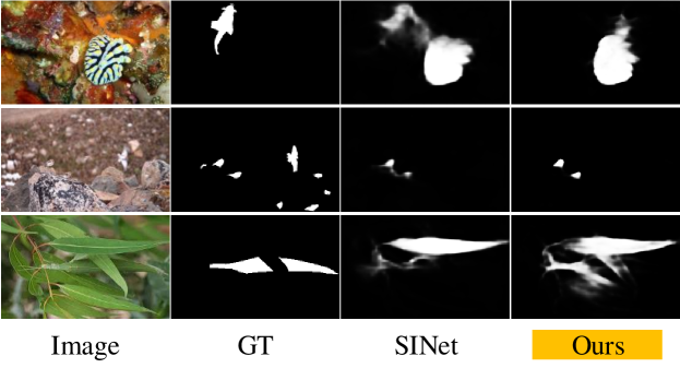
Figure 7: Failure cases. We show the failure cases for three challenging scenarios here.

4.6 Failure Cases

Fig. 7 shows some failure cases of our MCIF-Net. As can be observed, MCIF-Net fails in some challenging cases, where a large number of camouflaged objects exist and/or the image background is particularly complex. It is worth noting that the existing cutting-edge model also fails in these challenging cases. In the future, we will dedicate more efforts to improving the COD accuracy in these cases.

Table 3: Time efficiency analysis of different models. We use SINet [2] as the benchmark, and record the average promotion rates across three datasets compared with it.

Models	Training Time	Testing Time	$\Delta S_{\alpha}$	$\Delta E_{\phi}$	$\Delta F_{\beta}^{w}$	$\nabla M$
SINet [2]	70 min	0.2 s	-	-	-	-
CPD [37]	342 min	0.015 s	-0.024	-0.036	-0.043	-0.008
EGNet [25]	1670 min	0.031 s	-0.034	-0.027	-0.042	-0.005
MCIF-Net	55 min	0.027 s	+0.016	+0.066	+0.085	+0.009

4.7 Time Efficiency

We also investigate the time efficiency of our MCIF-Net by comparing it with a number of cutting-edge models, including SINet [2], and BASNet [27], EGNet [25]. All the experiments are performed on a computer equipped with an NVIDIA GeForce RTX 2080 GPU. The results, shown in Tab. 3, indicate that our model achieves the best accuracy with the shortest time in both training and testing. In particular, compared with the benchmark model SINet [2], our model significantly boosts performance, while reducing the testing time by nearly 10 times.

\begin{overpic}[width=303.53267pt]{Imgs/app1.pdf} \end{overpic}

Figure 8: Potential applications of MCIF-Net. A number of real object detection/segmentation tasks follow the same principle of COD. Therefore, our MCIF-Net can be a powerful solution to these tasks.

5 Discussions

Our MCIF-Net has shown remarkable performance in COD, which sufficiently demonstrates its practical value. Furthermore, we notice that a number of real object detection tasks are COD-like since they share the same principle with COD, where the under-detected object has a similar appearance with its surroundings.

For instance, the image, shown in the top left of Fig. 8, is an optical image used for industrial product quality control, while the corresponding label of under-detecting defect is shown in the top right. It can be observed that the defect looks very similar to its surrounding, which is consistent with our observations in the camouflaged images. Therefore, our MCIF-Net has great potentials for applying to this COD-like task and will be an effective solution for the defect detection [39].

Another good example is polyp segmentation [40]. As can be observed in the bottom row of Fig. 8, the boundaries between polyp and normal tissues are blurry, making it is hard to distinguish the polyp from the colonoscopy image. Our MCIF-Net can also be applied to this COD-like task, which will improve the segmentation accuracy effectively.

6 Conclusion and Future Work

In this paper, we propose MCIF-Net, a novel deep learning model for the accurate detection of camouflaged objects. MCIF-Net employs the specially-design DMC modules to extract rich context features from a large receptive field and effectively fuses the features using the proposed MIF modules. Our model provides both the large receptive field and effective fusion, effectively satisfying the demands of accurate COD. Extensive experiments on COD benchmark datasets demonstrate that MCIF-Net is capable of accurately detecting camouflaged objects and outperforms the SOTA methods. In addition, our ablation studies verify the effectiveness of two proposed modules, i.e., DMC and MIF, sufficiently.

In the future, we will explore compressing our model for a lightweight one suitable for mobile devices and further improving the efficiency of our model for real-time applications. In addition, as discussed in Section 5, our MCIF-Net has great potentials for a large number of COD-like tasks, e.g., defect detection and polyp segmentation. We will apply MCIF-Net to these tasks to advance the relevant fields.

References

- [1] G. H. Thayer, Concealing-coloration in the animal kingdom: an exposition of the laws of disguise through color and pattern: being a summary of Abbott H. Thayer’s discoveries, Macmillan Company, 1918.
- [2] D.-P. Fan, G.-P. Ji, G. Sun, M.-M. Cheng, J. Shen, L. Shao, Camouflaged object detection, in: Proceedings of the IEEE Conference on Computer Vision and Pattern Recognition, 2020.
- [3] S. Goferman, L. Zelnik-Manor, A. Tal, Context-aware saliency detection, IEEE transactions on pattern analysis and machine intelligence 34 (10) (2011) 1915–1926.
- [4] J. Long, E. Shelhamer, T. Darrell, Fully convolutional networks for semantic segmentation, in: Proceedings of the IEEE conference on computer vision and pattern recognition, 2015, pp. 3431–3440.
- [5] X. Zhang, C. Zhu, S. Wang, Y. Liu, M. Ye, A bayesian approach to camouflaged moving object detection, IEEE transactions on circuits and systems for video technology 27 (9) (2016) 2001–2013.
- [6] T.-N. Le, T. V. Nguyen, Z. Nie, M.-T. Tran, A. Sugimoto, Anabranch network for camouflaged object segmentation, Computer Vision and Image Understanding 184 (2019) 45–56.
- [7] H. Yousif, J. Yuan, R. Kays, Z. He, Fast human-animal detection from highly cluttered camera-trap images using joint background modeling and deep learning classification, in: 2017 IEEE international symposium on circuits and systems (ISCAS), IEEE, 2017, pp. 1–4.
- [8] A. C. Copeland, M. M. Trivedi, Signature strength metrics for camouflaged targets corresponding to human perceptual cues, Optical Engineering 37 (1998).
- [9] A. Owens, C. Barnes, A. Flint, H. Singh, W. Freeman, Camouflaging an object from many viewpoints, in: Proceedings of the IEEE Conference on Computer Vision and Pattern Recognition, 2014, pp. 2782–2789.
- [10] A. Mondal, Camouflaged object detection and tracking: A survey, International Journal of Image and Graphics 20 (04) (2020) 2050028.
- [11] H. Lamdouar, C. Yang, W. Xie, A. Zisserman, Betrayed by motion: Camouflaged object discovery via motion segmentation, in: Proceedings of the Asian Conference on Computer Vision, 2020.
- [12] J. Yan, T.-N. Le, K.-D. Nguyen, M.-T. Tran, T.-T. Do, T. V. Nguyen, Mirrornet: Bio-inspired adversarial attack for camouflaged object segmentation, arXiv preprint arXiv:2007.12881 (2020).
- [13] X. Wang, R. Girshick, A. Gupta, K. He, Non-local neural networks (2017).
- [14] J. Hu, L. Shen, G. Sun, Squeeze-and-excitation networks, in: Proceedings of the IEEE Conference on Computer Vision and Pattern Recognition, 2018, pp. 7132–7141.
- [15] L. Chen, H. Zhang, J. Xiao, L. Nie, J. Shao, W. Liu, T.-S. Chua, Sca-cnn: Spatial and channel-wise attention in convolutional networks for image captioning, in: Proceedings of the IEEE Conference on Computer Vision and Pattern Recognition, 2017, pp. 5659–5667.
- [16] J. Park, S. Woo, J.-Y. Lee, I. S. Kweon, Bam: Bottleneck attention module, arXiv preprint arXiv:1807.06514 (2018).
- [17] S. Woo, J. Park, J.-Y. Lee, I. So Kweon, Cbam: Convolutional block attention module, in: Proceedings of the European Conference on Computer Vision (ECCV), 2018, pp. 3–19.
- [18] J. Fu, J. Liu, H. Tian, Y. Li, Y. Bao, Z. Fang, H. Lu, Dual attention network for scene segmentation, in: Proceedings of the IEEE Conference on Computer Vision and Pattern Recognition, 2019, pp. 3146–3154.
- [19] X. Cao, A practical theory for designing very deep convolutional neural networks, Technical Report (2015).
- [20] K. He, X. Zhang, S. Ren, J. Sun, Spatial pyramid pooling in deep convolutional networks for visual recognition, IEEE Transactions on Pattern Analysis and Machine Intelligence 37 (9) (2014) 1904–16.
- [21] L.-C. Chen, G. Papandreou, I. Kokkinos, K. Murphy, A. L. Yuille, Deeplab: Semantic image segmentation with deep convolutional nets, atrous convolution, and fully connected crfs, IEEE transactions on pattern analysis and machine intelligence 40 (4) (2017) 834–848.
- [22] S. Liu, D. Huang, et al., Receptive field block net for accurate and fast object detection, in: Proceedings of the European Conference on Computer Vision (ECCV), 2018, pp. 385–400.
- [23] F. Yu, V. Koltun, Multi-scale context aggregation by dilated convolutions, arXiv preprint arXiv:1511.07122 (2015).
- [24] X. Glorot, A. Bordes, Y. Bengio, Deep sparse rectifier neural networks, in: Proceedings of the fourteenth international conference on artificial intelligence and statistics, 2011, pp. 315–323.
- [25] J.-X. Zhao, J.-J. Liu, D.-P. Fan, Y. Cao, J. Yang, M.-M. Cheng, Egnet: Edge guidance network for salient object detection, in: Proceedings of the IEEE Conference on Computer Vision and Pattern Recognition, 2019, pp. 8779–8788.
- [26] Z. Zhou, M. M. Rahman Siddiquee, N. Tajbakhsh, J. Liang, Unet++: A nested u-net architecture for medical image segmentation, in: DLMIA, 2018, pp. 3–11.
- [27] X. Qin, Z. Zhang, C. Huang, C. Gao, M. Dehghan, M. Jagersand, Basnet: Boundary-aware salient object detection, in: Proceedings of the IEEE Conference on Computer Vision and Pattern Recognition, 2019, pp. 7479–7489.
- [28] D.-P. Fan, M.-M. Cheng, Y. Liu, T. Li, A. Borji, Structure-measure: A new way to evaluate foreground maps, in: Proceedings of the IEEE Conference on Computer Vision and Pattern Recognition, 2017, pp. 4548–4557.
- [29] D.-P. Fan, C. Gong, Y. Cao, B. Ren, M.-M. Cheng, A. Borji, Enhanced-alignment measure for binary foreground map evaluation, International Joint Conferences on Artificial Intelligence (2018).
- [30] T. Lin, P. Dollar, R. Girshick, K. He, B. Hariharan, S. Belongie, Feature pyramid networks for object detection, in: Proceedings of the IEEE Conference on Computer Vision and Pattern Recognition, 2017, pp. 936–944.
- [31] K. He, G. Gkioxari, P. Dollár, R. Girshick, Mask R-CNN, in: IEEE ICCV, 2017, pp. 2961–2969.
- [32] H. Zhao, J. Shi, X. Qi, X. Wang, J. Jia, Pyramid scene parsing network, in: Proceedings of the IEEE Conference on Computer Vision and Pattern Recognition, 2017, pp. 6230–6239.
- [33] Liu, H. Nian, Y. Junwei, Ming-Hsuan, Picanet: Learning pixel-wise contextual attention for saliency detection, in: Proceedings of the IEEE Conference on Computer Vision and Pattern Recognition, 2018, pp. 3089–3098.
- [34] Z. Huang, L. Huang, Y. Gong, C. Huang, X. Wang, Mask scoring r-cnn, in: Proceedings of the IEEE Conference on Computer Vision and Pattern Recognition, 2019, pp. 6409–6418.
- [35] J.-J. Liu, Q. Hou, M.-M. Cheng, J. Feng, J. Jiang, A simple pooling-based design for real-time salient object detection, in: Proceedings of the IEEE Conference on Computer Vision and Pattern Recognition, 2019.
- [36] T. Zhao, X. Wu, Pyramid feature attention network for saliency detection, in: Proceedings of the IEEE Conference on Computer Vision and Pattern Recognition, 2019, pp. 3085–3094.
- [37] Wu, S. Zhe, H. Li, Qingming, Cascaded partial decoder for fast and accurate salient object detection, in: Proceedings of the IEEE Conference on Computer Vision and Pattern Recognition, 2019, pp. 3907–3916.
- [38] K. Chen, J. Pang, J. Wang, Y. Xiong, X. Li, S. Sun, W. Feng, Z. Liu, J. Shi, W. Ouyang, et al., Hybrid task cascade for instance segmentation, in: Proceedings of the IEEE Conference on Computer Vision and Pattern Recognition, 2019, pp. 4974–4983.
- [39] T. Wang, Y. Chen, M. Qiao, H. Snoussi, A fast and robust convolutional neural network-based defect detection model in product quality control, The International Journal of Advanced Manufacturing Technology 94 (9-12) (2018) 3465–3471.
- [40] D.-P. Fan, G.-P. Ji, T. Zhou, G. Chen, H. Fu, J. Shen, L. Shao, Pranet: Parallel reverse attention network for polyp segmentation, International Conference on Medical Image Computing and Computer-Assisted Intervention (2020).