Full Spectrum of the Liouvillian of Open Dissipative Quantum Systems in the Zeno Limit

Abstract

We consider an open quantum system with dissipation, described by a Lindblad Master equation (LME). For dissipation locally acting and sufficiently strong, a separation of the relaxation timescales occurs, which, in terms of the eigenvalues of the Liouvillian, implies a grouping of the latter in distinct vertical stripes in the complex plane at positions determined by the eigenvalues of the dissipator. We derive effective LME equations describing the modes within each stripe separately, and solve them perturbatively, obtaining for the full set of eigenvalues and eigenstates of the Liouvillian explicit expressions correct at order $1/\Gamma$ included, where $\Gamma$ is the strength of the dissipation. As an example, we apply our general results to quantum $XYZ$ spin chains coupled, at one boundary, to a dissipative bath of polarization.

Recently a great deal of analytic progress has been made in the theory of open quantum systems and their steady-state exact solutions. Much less is known about the full spectrum of the Liouvillian [the Lindbladian, more precisely, if the open quantum system is described, as very often happens, by a Lindblad master equation (LME)]. Just to say, the knowledge of this spectrum is essential to predict the finite-time evolution of dissipative systems, as of interest in fields ranging from quantum computing QuantumComputing to quantum biology QuantumBiology . The problem basically remains intractable, except via hard computational methods Briegel.Englert ; Barnett.Stenholm ; Rocca2008 ; Torres.Betzholz.Bienert .

The existing literature regarding the Liouvillian general properties focuses on an analysis of asymptotic time regime $t\to\infty$, i.e., putting emphasis on the existence of a decoherence-free subspace and the asymptotic leakage out of it Marcuzzi.etal ; GeometryAndResponse ; Shpielberg . Within such an approach, however, a substantial part of information about the Liouvillian spectrum is lost.

Exceptionally, under special conditions imposed on the Lindblad operators and the Hamiltonian, the Liouvillian spectrum can be related to the spectrum of auxiliary non-Hermitian operators. However, even in this case, the complete set of eigenstates is out of reach MEP ; Kurlov ; BBMJ ; NKM .

In the present communication, in contrast, we show how to obtain the complete set of eigenvalues and eigenstates of the Liouvillian, provided that the dissipation is sufficiently strong with respect to the coherent part of the evolution, in the so-called quantum Zeno regime Misra1977 ; POT1996 ; ZenoStaticsExperimentalReview ; ZenoPascazio2020 . For this setup to be nontrivial, dissipation must act only on a part of the degrees of freedom.

As we will see, in the limit of strong dissipation acting on a part of degrees of freedom, the behavior of an open quantum system simplifies and the full Liouvillian can be block diagonalized.

We provide a general procedure to obtain the full set of eigenvalues and eigenstates by means of a perturbative approach in terms of the solution of a linear problem for the dissipation-projected Hamiltonian 2018ZenoDynamics ; 2014Venuti , and other related Hamiltonians acting in a reduced Hilbert space. As an example, we comprehensively discuss the case of general open $XYZ$ spin chains with arbitrary spin states targeted at one of the boundaries by the strong interaction with dissipative environments.

General theory.—We Considery an open quantum system with finite Hilbert space $\mathcal{H}$ and dissipation acting only on a part of its degrees of freedom, namely, those associated to the subspace $\mathcal{H}_{0}\subset\mathcal{H}$. Denoting by $\mathcal{H}_{1}$ the dissipation-free subspace, we have $\mathcal{H}=\mathcal{H}_{0}\otimes\mathcal{H}_{1}$ with $\dim\mathcal{H}_{0}=d_{0}$, $\dim\mathcal{H}_{1}=d_{1}$ and $d_{0}d_{1}=d=\dim\mathcal{H}$. The evolution of the reduced density matrix operator of the systems, $d\rho(\tau)/d\tau=\mathcal{L}[\rho(\tau)]$, is determined by the Liouvillian

$$\mathcal{L}[\cdot]=-i[H,\cdot]+\Gamma\mathcal{D}[\cdot],$$ (1)

where $H$ is the Hamiltonian of the system, $\mathcal{D}[\cdot]$ a Lindblad dissipator of standard form and $\Gamma$ the strength of the dissipation. The use of a Markovian Lindblad dynamics for large dissipation is justified for reservoirs with very short correlation times Gorini . Note that we work in units of $\hbar=1$, i.e., $\tau=t_{\mathrm{ph}}/\hbar$ and $\Gamma=\Gamma_{\mathrm{ph}}\hbar$, where $t_{\mathrm{ph}}$ and $\Gamma_{\mathrm{ph}}$ are the physical time and dissipation strength.

In Ref. 2018ZenoDynamics it has been shown that in the Zeno limit $\Gamma\to\infty$ the dynamics (1) is still reduced to a new Lindblad equation written in terms of a renormalized Hamiltonian and an effective dissipator. More precisely, for times $\tau\gg 1/\Gamma$ and with an error $O(1/\Gamma^{2})$ we have $\rho(\tau)=\psi_{0}\otimes R_{0}(\tau)$, where $\psi_{0}\in\mathcal{H}_{0}$ is the dissipator kernel, $\mathcal{D}[\psi_{0}]=0$, (assumed to be unique) and $R_{0}(\tau)\in\mathcal{H}_{1}$ satisfies

$$\frac{dR_{0}(\tau)}{d\tau}=-i[h_{D}+\tilde{H}_{a}/\Gamma,R_{0}(\tau)]+\frac{1}{\Gamma}\tilde{\cal D}[R_{0}(\tau)].$$ (2)

The effective Hamiltonian $\tilde{H}=h_{D}+\tilde{H}_{a}/\Gamma$ is the sum of the dissipation-projected Hamiltonian, $h_{D}=\mathop{\mathrm{tr}_{\mathcal{H}_{0}}}\limits((\psi_{0}\otimes I_{\mathcal{H}_{1}})H)$, and a Lamb shift correction $\tilde{H}_{a}$. With $\mathop{\mathrm{tr}_{\mathcal{H}_{0}}}\limits$ we indicate the trace in the subspace $\mathcal{H}_{0}$. Note that both $\tilde{H}_{a}$ and the effective dissipator $\tilde{\cal D}[\cdot]$ act in the sole subspace $\mathcal{H}_{1}$. Explicit expressions of $\tilde{H}_{a}$ and $\tilde{\cal D}[\cdot]$ are given in [6] and, for convenience, reported in Supplemental Material SM .

Equation (2) provides a complete information about $R_{0}$, the dissipation-free component of the density matrix $\rho$. The full density matrix has, however, an expansion of the form $\rho(\tau)=\sum_{k}\psi_{k}\otimes R_{k}(\tau)$, where $\psi_{k}$ are the eigenstates of the original dissipator $\mathcal{D}$ (which we assume diagonalizable),

$$\mathcal{D}[\psi_{k}]=c_{k}\psi_{k}.$$ (3)

The complex eigenvalues $c_{k}$ always have a nonpositive real part and one of them is 0, conventionally, $c_{0}=0$. When $\Gamma$ is large, all the components $k>0$ of the density matrix lying outside the dissipation-free subspace can be shown to scale as $1/\Gamma$, namely, $||R_{k}(\tau)||=O(1/\Gamma)$ for $\tau>O(1)$, see 2014Venuti .

The spectrum of the effective Liouvillian $\tilde{\mathcal{L}}$ associated to Eq. (2) gives only a part of the full Liouvillian spectrum, namely, $d_{1}^{2}$ eigenvalues out of $d^{2}=(d_{0}d_{1})^{2}$. The remaining $d^{2}-d_{1}^{2}$ eigenvalues of the Liouvillian $\mathcal{L}$ originate from the components $R_{k}$ with $k>0$ in the expansion of the full density matrix.

In 2018ZenoDynamics it has been shown how to obtain, in the Zeno limit, the nonequilibrium steady state, i.e., the eigenstate of $\mathcal{L}$ corresponding to the eigenvalue $0$. Here, we derive explicit formulas for all the eigenvalues and eigenstates of $\mathcal{L}$ near the Zeno limit, up to order $1/\Gamma$ included. Explicitly, we will first obtain equations analogous to Eq. (2) for all the components $R_{k}(\tau)$ of the density matrix, and then show how to use these equations to derive eigenvalues and eigenstates of $\mathcal{L}$.

In order to formulate our main statement, note that the dissipator eigenstates $\{\psi_{k}\}$ of Eq. (3) form a basis in $\mathcal{H}_{0}$. Let $\{\varphi_{k}\}$ be a biorthogonal basis in $\mathcal{H}_{0}$ satisfying $\mathop{\mathrm{tr}}\limits(\psi_{k}\varphi_{n})=\delta_{kn}$. The decompositions of the Hamiltonian $H$ and of the density matrix $\rho(\tau)$ in the bases $\{\varphi_{k}\}$ and $\{\psi_{k}\}$ are, respectively,

$$H=\sum_{m}(\varphi_{m}^{\dagger}\otimes g_{m}^{\dagger})=\sum_{m}(\varphi_{m}\otimes g_{m}),$$ (4)

$$\qquad g_{m}=\mathop{\mathrm{tr}_{\mathcal{H}_{0}}}\limits((\psi_{m}\otimes I_{\mathcal{H}_{1}})H),$$ (5)

$$\rho(\tau)=\sum_{k}\psi_{k}\otimes R_{k}(\tau),$$ (6)

$$\qquad R_{k}(\tau)=\mathop{\mathrm{tr}_{\mathcal{H}_{0}}}\limits((\varphi_{k}\otimes I_{\mathcal{H}_{1}})\rho(\tau)).$$ (7)

Statement.—The component $R_{k}$ corresponding to a nonzero dissipator eigenvalue $c_{k}$ with degeneracy $\mathrm{deg}$, near the Zeno limit satisfy

$$\frac{dR_{k}}{d\tau}= \ \Gamma c_{k}R_{k}+i\sum_{s:c_{s}=c_{k}}\left(U_{k,s}R_{s}-R_{s}W_{k,s}\right)$$

$$+\frac{1}{\Gamma}\sum_{z>0}\sum_{m>0}\sum_{n:c_{n}\neq c_{k}}\sum_{s:c_{s}=c_{k}}\frac{1}{c_{n}-c_{k}}$$

$$\qquad\times\Big{(}-\gamma^{n,s,k}_{m,z}g_{m}R_{s}g_{z}^{\dagger}+\varepsilon^{n,s,k}_{z,m}g_{z}^{\dagger}g_{m}R_{s}$$

$$\qquad\qquad+\delta^{n,s,k}_{z,m}R_{s}g_{z}^{\dagger}g_{m}\Big{)}+O(1/\Gamma^{2}),$$ (8)

where $U_{k,s}$ and $W_{k,s}$ are operators in $\mathcal{H}_{1}$ given by

$$U_{k,s}=\sum_{n}B_{n,s,k}g_{n}^{\dagger},\quad W_{k,s}=\sum_{n}A_{n,s,k}g_{n}^{\dagger}$$ (9)

and $\gamma^{n,s,k}_{m,z}$, $\varepsilon^{n,s,k}_{m,z}$ and $\delta^{n,s,k}_{m,z}$ are the coefficients

$$\gamma^{n,s,k}_{m,z}=C_{m,s,n}A_{z,n,k}+A_{z,s,n}C_{m,n,k},$$ (10)

$$\epsilon^{n,s,k}_{z,m}=C_{m,s,n}B_{z,n,k},$$ (11)

$$\delta^{n,s,k}_{z,m}=A_{z,s,n}C_{k,n,m},$$ (12)

with

$$A_{m,k,n}=\mathop{\mathrm{tr}}\limits(\varphi_{n}\psi_{k}\varphi_{m}^{\dagger}),$$ (13)

$$B_{m,k,n}=\mathop{\mathrm{tr}}\limits(\varphi_{n}\varphi_{m}^{\dagger}\psi_{k}),$$ (14)

$$C_{m,k,n}=\mathop{\mathrm{tr}}\limits(\varphi_{n}\varphi_{m}\psi_{k}).$$ (15)

Note that the above coefficients are related to the dissipator via its eigenstates $\{\psi_{k}\}$ and the associated biorthogonal basis $\{\varphi_{k}\}$. For a nondegenerate eigenvalue, $\mathrm{deg}=1$, only the simplified operators $U_{k,k}=U_{k}$ and $W_{k,k}=W_{k}$ appear in Eq. (Full Spectrum of the Liouvillian of Open Dissipative Quantum Systems in the Zeno Limit), where

$$U_{k}=g_{0}+\sum_{n>0}B_{n,k,k}g_{n}^{\dagger},\quad W_{k}=g_{0}+\sum_{n>0}A_{n,k,k}g_{n}^{\dagger}.$$ (16)

Equation (Full Spectrum of the Liouvillian of Open Dissipative Quantum Systems in the Zeno Limit) applies also in the presence of more degenerate eigenvalues.

The above statement follows from a perturbative Dyson expansion with respect to the small parameter $1/\Gamma$ of the Liouvillian equation for $\rho(t)$, where $t$ is the scaled time $t=\Gamma\tau$. With this scaling, we have $d\rho(t)/dt={\cal L}_{0}[\rho(t)]+K[\rho(t)]$, where ${\cal L}_{0}[\cdot]=\mathcal{D}[\cdot]$ and $K[\cdot]=-(i/\Gamma)[H,\cdot]$. The corresponding exact propagator, namely, $\exp(({\cal L}_{0}+K)t)$, can be expanded in a Dyson series with respect to the perturbation $K$. Keeping the expansion terms up to order $K^{2}$ included and coming back to the time $\tau$, after some algebra, we get Eq. (Full Spectrum of the Liouvillian of Open Dissipative Quantum Systems in the Zeno Limit). Full details of the proof are given in Supplemental Material SM .

Eigenvalues and eigenvectors of $\mathcal{L}$.—By finding the normal modes of the linear problem (Full Spectrum of the Liouvillian of Open Dissipative Quantum Systems in the Zeno Limit) for each index $k>0$, as well as of the linear problem (2) for $k=0$, we obtain all the eigenvalues of the Liouvillian $\mathcal{L}$. Let $\lambda_{k,\alpha,\beta}$ be the set of the eigenvalues of $\mathcal{L}$ corresponding to $c_{k}$. First consider a nondegenerate $c_{k}$. In the limit $\Gamma\rightarrow\infty$, the $O(1/\Gamma)$ contributions in Eq. (Full Spectrum of the Liouvillian of Open Dissipative Quantum Systems in the Zeno Limit) can be neglected and, expanding $R_{k}(\tau)=\sum_{\alpha,\beta}c_{\alpha\beta}(\tau)|\alpha\rangle\langle\tilde{\beta}|$, where $|\alpha\rangle$ are the right eigenvectors of $U_{k}$ with eigenvalues $u_{\alpha}$ and $\langle\tilde{\beta}|$ are the left eigenvectors of $W_{k}$ with eigenvalues $w_{\beta}$, we find $dc_{\alpha\beta}(\tau)/d\tau=\lambda_{k,\alpha,\beta}c_{\alpha\beta}(\tau)=(c_{k}\Gamma+i(u_{\alpha}-w_{\beta}))c_{\alpha\beta}(\tau)$. This implies

$$\lambda_{k,\alpha,\beta}=c_{k}\Gamma+i(u_{\alpha}-w_{\beta})+O(1/\Gamma),$$ (17)

with corresponding eigenvectors $\psi_{k,\alpha,\beta}=\psi_{k}\otimes|\alpha\rangle\langle\tilde{\beta}|$. Note that, even if not explicitly indicated, the eigenvalues $w_{\alpha}$ and $u_{\beta}$ depend, as the corresponding eigenvectors do, on the index $k$.

The $1/\Gamma$ corrections to the eigenvalues (17) are then found by a standard perturbative formula, $\delta\lambda_{k,\alpha,\beta}=\langle R_{\alpha\beta}|\hat{V}_{k}|R_{\alpha\beta}\rangle$, where $\hat{V}_{k}$ is the vectorized form of the $O(1/\Gamma)$ term in the superoperator of Eq. (Full Spectrum of the Liouvillian of Open Dissipative Quantum Systems in the Zeno Limit) and $|R_{\alpha\beta}\rangle$ is an eigencomponent of the reduced density matrix $|R_{\alpha\beta}\rangle=|\alpha\rangle\otimes|\tilde{\beta}\rangle^{*}$. Every perturbative term of type $Q|x\rangle\langle y|P$ in (Full Spectrum of the Liouvillian of Open Dissipative Quantum Systems in the Zeno Limit) gives a contribution $\mathop{\mathrm{tr}}\limits(Q|x\rangle\langle y|P|y\rangle\langle x|)=\langle x|Q|x\rangle\langle y|P|y\rangle$ to the eigenvalue correction. Explicitly, we obtain

$$\delta\lambda_{k,\alpha,\beta}=\ \frac{1}{\Gamma}\sum_{z>0}\sum_{m>0}\sum_{n:c_{n}\neq c_{k}}\frac{1}{c_{n}-c_{k}}\Big{(}-\gamma^{n,n,k}_{m,z}\langle\alpha|g_{m}|\alpha\rangle$$

$$\times\langle\tilde{\beta}|g_{z}^{\dagger}|\tilde{\beta}\rangle+\varepsilon^{n,n,k}_{z,m}\langle\alpha|g_{z}^{\dagger}g_{m}|\alpha\rangle+\delta^{n,n,k}_{z,m}\langle\tilde{\beta}|g_{z}^{\dagger}g_{m}|\tilde{\beta}\rangle\Big{)}.$$ (18)

The $O(1/\Gamma)$ corrections to the respective eigenstates $\psi_{k}\otimes|\alpha\rangle\langle\tilde{\beta}|$ are also given by standard first-order perturbative formulas Landau .

Of course, the above $1/\Gamma$ correction is valid if the eigenvalues (17) are nondegenerate. In the case of $\lambda_{k,\alpha,\beta}$ degenerate, a different, although still standard, procedure must be undertaken (diagonalization within the subspace of degeneration) to obtain the $1/\Gamma$ corrections. Explicit expressions will be given for the case study considered below.

The case of a degenerate dissipator eigenvalue $c_{k}$ can be tackled in a similar way.

A case study: The $XYZ$ spin chain.—We illustrate the above results on a Heisenberg spin chain with $N+1$ sites, the first one being in contact with a strongly dissipative environment. The coherent part of the evolution is given by the standard $XYZ$ Hamiltonian $H=\sum_{j=0}^{N-1}\sum_{\alpha=x,y,z}\sigma_{j}^{\alpha}J_{\alpha}\sigma_{j+1}^{\alpha}$, $\sigma_{j}^{\alpha}$ being the $\alpha$-th Pauli matrix acting at site $j$, whereas dissipation acts locally on site $0$ and targets an arbitrary, pure or mixed, single spin state $\rho_{0}$ at this site Prosen2011 . The evolution of the the density matrix $\rho(\tau)$ of the full chain is determined by a LME with Liouvillian as in Eq. (1). The Lindblad dissipator acting on spin $1$ is the sum of two terms, $\mathcal{D}=((1+\mu)/2)\mathcal{D}_{1}+((1-\mu)/2)\mathcal{D}_{2}$,

$$\mathcal{D}_{\alpha}[\rho]=L_{\alpha}\rho L_{\alpha}^{\dagger}-\frac{1}{2}L_{\alpha}^{\dagger}L_{\alpha}\rho-\frac{1}{2}\rho L_{\alpha}^{\dagger}L_{\alpha},\quad\alpha=1,2,$$ (19)

where $L_{1}=|s(\theta,\varphi)\rangle\langle s^{\perp}(\theta,\varphi)|$ and $L_{2}=L_{1}^{\mathrm{T}}$, with $|s(\theta,\varphi)\rangle=\cos(\theta/2)e^{-i\varphi/2}|{\uparrow}\rangle+\sin(\theta/2)e^{i\varphi/2}|{\downarrow}\rangle$ and $\langle s(\theta,\varphi)|s^{\perp}(\theta,\varphi)\rangle=0$. This dissipator targets the polarization $\mu\vec{n}_{0}$ on site $0$, where $\vec{n}_{0}$ is the unit vector $\vec{n}_{0}=(\sin\theta\cos\varphi,\sin\theta\sin\varphi,\cos\theta)$. The uniqueness of the nonequilibrium stationary state (NESS) can be proven using Evans criterion Evans .

Striped structure of spectrum. The distribution of the Liouvillian eigenvalues manifestly depends on the strength of dissipation $\Gamma$ in Eq. (1). For medium dissipation strengths, comparable with the exchange integral in the model, the eigenvalues are scattered seemingly randomly, see Fig. 1 (top). For large $\Gamma$, they are arranged in distinct stripes, see Fig. 1 (bottom). The stripelike structure stems from the properties of the dissipator in the LME. In fact, the eigenvalue problem (3) of the locally acting dissipator $\mathcal{D}$ can be easily solved 2018ZenoDynamics , yielding

$$\begin{array}[]{ll}c_{0}=0,&\psi_{0}=\frac{1+\mu}{2}|s\rangle\langle s|+\frac{1-\mu}{2}|s^{\perp}\rangle\langle s^{\perp}|,\\ c_{1}=-\frac{1}{2},&\psi_{1}=|s\rangle\langle s^{\perp}|,\\ c_{2}=-\frac{1}{2},&\psi_{2}=|s^{\perp}\rangle\langle s|,\\ c_{3}=-1,&\psi_{3}=|s\rangle\langle s|-|s^{\perp}\rangle\langle s^{\perp}|.\end{array}$$ (24)

where $|s\rangle\equiv|s(\theta,\varphi)\rangle$. The respective biorthogonal basis $\{\varphi_{k}\}$ is given by

$$\begin{array}[]{l}\varphi_{0}=I_{\mathcal{H}},\qquad\varphi_{1}=\psi_{2},\qquad\varphi_{2}=\psi_{1},\\ \varphi_{3}=\frac{1-\mu}{2}|s\rangle\langle s|-\frac{1+\mu}{2}|s^{\perp}\rangle\langle s^{\perp}|.\end{array}$$ (27)

Neglecting the coherent part provided by the Hamiltonian $H$, the Liouvillian $\mathcal{L}$ of Eq. (1) would have the eigenvalues $\Gamma c_{k}$, $k=0,\dots,3$, each eigenvalue having a degeneracy $2^{2N}$ due to the inclusion of the $N$ extra spins. Adding $H$ acts as a perturbation (the small parameter being $1/\Gamma$), which results in lifting the degeneracies. The perturbation-affected eigenvalues have, therefore, real part approximately given by $\Gamma c_{k}$.

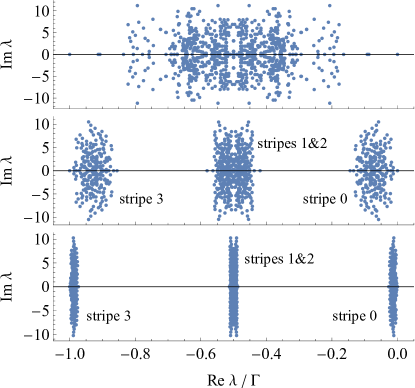
Figure 1: (color online) Exact complex eigenvalues of the Liouvillian evaluated numerically for $\Gamma=0.5,\ 8,\ 20$ (from top to bottom). Increasing $\Gamma$, eigenvalues arrange in stripes whose number equals that of the eigenvalues of the dissipator. For $\Gamma$ large, the width of the stripes scales as $1/\Gamma$ while their height remains constant; the distance between the stripes scales as $\Gamma$. Parameters: $N=4,\vec{J}=(1,1,-0.6058)$, $\varphi=0$, $\theta=\pi/2$, $\mu=1$.

Spectra of the stripes.—The stripe associated to $c_{0}=0$ is described by the equation for $R_{0}$ considered in 2018ZenoDynamics ; ZenoStatics . We review this equation and evaluate the corresponding spectrum in SM . The other Zeno stripes are associated with the nonzero eigenvalues of the dissipator (24): $c_{1}=c_{2}=-1/2$ and $c_{3}=-1$. In the following, we consider the eigenvalue $c_{3}$. The analysis of the degenerate eigenvalue $c_{1}=c_{2}$ is similar and detailed in SM .

To evaluate the $O(1)$ terms of Eq. (Full Spectrum of the Liouvillian of Open Dissipative Quantum Systems in the Zeno Limit) for $k=3$, we need the operators $U_{3}$ and $W_{3}$ (16). The only nonzero coefficients $A_{n,3,3}$ and $B_{n,3,3}$ with $n>0$ are $A_{3,3,3}=B_{3,3,3}=-\mu$ and we find $U_{3}=W_{3}=g_{0}-\mu g_{3}^{\dagger}=\sum_{j=1}^{N-1}h_{j,j+1}-\mu(J\vec{n}_{0})\cdot\vec{\sigma}_{1}$, where $h_{j,j+1}=\vec{\sigma}_{j}\cdot(J\vec{\sigma}_{j+1})$ is the local density of the Hamiltonian $H$. Comparing $U_{3}$ and $h_{D}$, we see that they differ just by the sign of the local field acting on site $1$. It can be shown that $h_{D}$ and $U_{3}$ are, therefore, isospectral SM . According to (17), the corresponding Liouvillian eigenvalues are

$$\lambda_{3,\alpha,\beta}=-\Gamma+i(\epsilon_{\alpha}-\epsilon_{\beta})+O(1/\Gamma)$$ (28)

and the corresponding eigenvectors are $\psi_{3,\alpha,\beta}=|\psi_{3}\rangle\otimes|\alpha\rangle\langle\beta|+O(1/\Gamma)$, where $|\alpha\rangle$ is an eigenvector of $U_{3}$ with eigenvalue $\epsilon_{\alpha}$. The corrections $O(1/\Gamma)$ are evaluated according to Eq. (18) for $\beta\neq\alpha$. The case $\beta=\alpha$ is similar to the calculation done for $c_{0}=0$ and is detailed in SM .

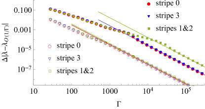
Figure 2: Standard deviation of the modulus of the difference between numerically obtained Liouvillian eigenvalues and our perturbative prediction as a function of $\Gamma$, separately for each stripe. The set of data corresponding to empty symbols is obtained with parameters as in Fig. 1 (pure target state). The set with filled symbols corresponds to a mixed target state with parameters: $N=4,\vec{J}=(1,1.7,-0.137)$, $\varphi=0$, $\theta=2\pi/7$, $\mu=-0.7$. The straight lines are $(\Gamma_{c}/\Gamma)^{2}$ with, from top to bottom, $\Gamma_{c}=129,\leavevmode\nobreak\ 51,\leavevmode\nobreak\ 6.3,\leavevmode\nobreak\ 5.6$.

Figure 2 shows, stripe by stripe, the standard deviation of the error obtained by comparing the numerically computed Liouvillian eigenvalues with our perturbative eigenvalues, order $O(1/\Gamma)$ included. As expected, this error behaves like $(\Gamma_{c}/\Gamma)^{2}$ for $\Gamma$ sufficiently large, with $\Gamma_{c}$ possibly different for the various stripes depending on the parameters chosen. The value of $\Gamma_{c}$ can be used as an indicator of an onset of the Zeno regime, characterized by the appearance of stripes in Fig. 1. From Fig. 2 we also see that the Zeno regime is reached easier for larger boundary gradient $|\mu|$.

Our Zeno-limit expansion for an eigenvalue $\lambda$ is applicable if the dissipation $\Gamma$ is much larger than the inverse radius of convergence of the $1/\Gamma^{k}$ perturbative series for $\lambda$. The global radius of convergence, valid for all Liouvillian eigenvalues, is problem specific. In Fig. 3 we show, as a function of $\Gamma$, the real part of all Liouvillian eigenvalues of a Heisenberg chain with $2$ spins, the first spin being targeted by a $z$-polarizing dissipation. Depending on the anisotropy, we find up to eight exceptional points, where two or more eigenvalues coalesce EP-Kato ; EP-Review ; EP-Heiss ; EP-Hatano . Fully analytical Zeno regime sets in beyond the rightmost branching point, see Fig. 3.

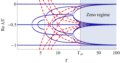
Figure 3: Rescaled real part of all Liouvillian eigenvalues versus $\Gamma$, for $N=1$. Parameters: $\vec{J}=(1,2.3,-0.61)$, $\varphi=\theta=0$ and $\mu=1$. Dashed lines show the near Zeno-limit predictions detailed in SM . The vertical line at $\Gamma_{\mathrm{cr}}$ marks the location of the rightmost branching points where Zeno regime sets in.

Let us summarize our findings. The eigenvalues of a Liouvillian with a locally acting dissipator at large dissipation strength $\Gamma$ are arranged in a set of stripes, see Fig. 1, indicating the existence of a hierarchy of relaxation timescales in the system HyerarchyRelaxationTimescales . The number of stripes coincides with the number of different eigenvalues of the Lindblad dissipator $\mathcal{D}$ in (1).

The width of the stripes scales as $1/\Gamma$ and the distance between the stripes scales as $\Gamma$. The vertical extension of the stripes does not depend on $\Gamma$ and is of the order of the norm $||H||$ of the coherent part of the Liouvillian (1). The position of the stripes on the real axis is $\mathop{\rm Re}\lambda=c_{k}\Gamma+O(1/\Gamma)$ where $c_{k}$ are the eigenvalues of the dissipator (3). Each stripe corresponding to a nondegenerate $c_{k}$ contains $d_{1}^{2}$ Liouvillian eigenvalues, where $d_{1}=\dim{\cal H}_{1}$ is the dimension of that part of Hilbert space which is not affected directly by the dissipation. Emergence of stripes can be viewed as a hallmark of a quantum Zeno regime.

We derived linear spectral problems for the dissipation-projected Liouvillian, for each relaxation mode $c_{k}$, and outlined a complete solution of the eigenvalue problem via a perturbative analysis. We demonstrated our general results in the case of dissipation acting on a single boundary qubit of an anisotropic Heisenberg spin chain. For this case, we obtained explicit expressions for eigenvalues and eigenvectors of the problem near the Zeno regime. The solutions are given in terms of spectral data of a dissipation-projected Hamiltonian and other similar Hamiltonians, these being much simpler objects than the original Liouvillian. Our method is straightforwardly applicable to the $XYZ$ model with dissipation acting on both boundaries, thus creating boundary gradients 2020ZenoPRL ; 2020ZenoPRE , which play a prominent role in studies of quantum transport 2020BertiniQuantumTransport . All the auxiliary Hamiltonians have the form of an open $XYZ$ spin chain with boundary fields and are integrable OffDiagonal .

To derive our results we used several assumptions: (i) diagonalizability of the dissipator (3), (ii) uniqueness of its kernel, (iii) absence of anomalous scaling of the gaps in the spectrum of the Liouvillian, including the Liouvillian gap. A generalization of our results is, in principle, straightforward. We expect the emergence of striped structure and scaling of the stripes in the Zeno limit to be qualitatively correct also for degenerate kernels, e.g., for those resulting from Hermitian Lindblad operators RandomLiuLindbladOperatorsHermitian .

Our explicit results shed a light on the intrinsic properties of an isolated system coupled strongly to the environment, and make its study almost analytically affordable.

Supplemental Material for
Full spectrum of open dissipative quantum systems in the Zeno limit

Vladislav Popkov and Carlo Presilla

Appendix A Lamb shift Hamiltonian and effective dissipator of Eq. (2)

Assume that the kernel of $\mathcal{D}$ is one-dimensional, i.e., its 0 eigenvalue, $\mathcal{D}[\psi_{0}]=0$, is nondegenerate and $\mathcal{D}$ is diagonalizable, i.e., there exists a basis $\{\psi_{k}\}$ (not necessarily orthogonal) such that $\mathcal{D}[\psi_{k}]=c_{k}\psi_{k}$. Let $\{\varphi_{k}\}$ be a complementary basis, trace-orthonormal to the basis $\{\psi_{k}\}$, $\mathop{\mathrm{tr}}\limits(\varphi_{k}\psi_{j})=\delta_{k,j}$. In Ref. 2018ZenoDynamics it has been shown that

$$\tilde{H}_{a}=\sum_{m>0}\sum_{n>0}\beta_{m,n}g_{m}^{\dagger}g_{n},$$ (S1)

$$\tilde{\mathcal{D}}[\cdot]=\sum_{m>0}\sum_{n>0}\gamma_{m,n}\left(g_{n}\cdot g_{m}^{\dagger}-\frac{1}{2}g_{m}^{\dagger}g_{n}\cdot-\frac{1}{2}\cdot g_{m}^{\dagger}g_{n}\right),$$ (S2)

where $g_{k}=\mathop{\mathrm{tr}_{\mathcal{H}_{0}}}\limits((\psi_{k}\otimes I_{\mathcal{H}_{1}})H)$ are the operators in Eq. (5) and $\gamma_{m,n}=Y_{m,n}+Y_{n,m}^{*}$ and $\beta_{m,n}=(Y_{m,n}-Y_{n,m}^{*})/(2i)$ with $Y_{m,n}=-\mathop{\mathrm{tr}}\limits\left(\varphi_{m}^{\dagger}\varphi_{n}\psi_{0}\right)/c_{m}^{*}$ are the elements of two matrices which are, respectively, positive and Hermitian. Note that the dissipation-projected Hamiltonian of Eq. (2) is $h_{D}=g_{0}$.

For the dissipator $\mathcal{D}=((1+\mu)/2)\mathcal{D}_{1}+((1-\mu)/2)\mathcal{D}_{2}$ with $\mathcal{D}_{1}$ and $\mathcal{D}_{2}$ given by Eq. (19), we have $\beta_{m,n}=0$ and $\gamma_{m,n}=\gamma_{m}\delta_{m,n}$, where $\gamma_{1}=(1+\mu)/2$, $\gamma_{2}=(1-\mu)/2$ and $\gamma_{3}=(1-\mu^{2})/4$.

Appendix B Proof of Statement: nondegenerate eigenvalues

We start introducing the spectral projection $P_{k}$ according to

$$P_{k}X =\psi_{k}\otimes X_{k},\qquad X_{k}=\mathop{\mathrm{tr}_{\mathcal{H}_{0}}}\limits\left((\varphi_{k}\otimes I_{\mathcal{H}_{1}})X\right).$$ (S3)

We have $P_{k}P_{m}=\delta_{k,m}P_{m}$ and $P_{k}\rho(\tau)=\psi_{k}\otimes R_{k}(\tau)$. From Eq. (1), scaling the time by $\tau=t/\Gamma$, we find $d\rho(t)/dt={\cal L}_{0}[\rho(t)]+K[\rho(t)]$ with ${\cal L}_{0}[\cdot]=\mathcal{D}[\cdot]$ and $K[\cdot]=-(i/\Gamma)[H,\cdot]$. If we now apply the Liouvillian propagator $\epsilon_{t}=\exp\mathcal{L}t$ on $P_{k}$ with $k>0$, we can use the Dyson expansion with respect to the small perturbation $K$ and obtain

$$\epsilon_{t}P_{k}= \ e^{c_{k}t}\left(P_{k}+P_{k}KP_{k}t\right)+\frac{1}{c_{k}}P_{0}KP_{k}(e^{c_{k}t}-1)$$

$$+\!\!\!\!\!\!\!\sum_{m>0,\leavevmode\nobreak\ m\neq k}\frac{e^{c_{m}t}}{c_{k}-c_{m}}P_{m}KP_{k}(e^{(c_{k}-c_{m})t}-1)+O(K^{2}).$$ (S4)

The term $P_{0}KP_{k}$ describes the flow towards the dissipation-free subspace; as expected, its norm is of order $1/\Gamma$ due to presence of $K$. The term in (S4) containing $P_{m}KP_{k}$ describes the intra-sector flow $\psi_{k}\otimes R_{k}(0)\rightarrow\psi_{m}\otimes R_{m}(t)$, and is at most of order $1/\Gamma$ at any time. Finally, the inter-sector flow $\psi_{k}\otimes R_{k}(0)\rightarrow\psi_{k}\otimes R_{k}(t)$ is given by the first two terms, namely,

$$P_{k}\epsilon_{t}P_{k}=e^{c_{k}t}\left(P_{k}+P_{k}KP_{k}t\right)+O(K^{2}).$$ (S5)

The evolution $R_{k}(0)\rightarrow R_{k}(t)$ resulting from Eq. (S5) can be cast in differential form by using $dR_{k}(t)/dt=\lim_{t\rightarrow 0}(R_{k}(t)-R_{k}(0))/t$. Applying $P_{k}\epsilon_{t}P_{k}$ on $\rho(t)$ we find $\psi_{k}\otimes dR_{k}(t)/dt=c_{k}\psi_{k}\otimes R_{k}+P_{k}KP_{k}\rho(t)$. Scaling back the time by $t=\Gamma\tau$, after some algebra we get

$$\frac{dR_{k}(\tau)}{d\tau}= \ \Gamma c_{k}R_{k}(\tau)+i[g_{0},R_{k}(\tau)]$$

$$+i\sum_{n>0}\left(\mathop{\mathrm{tr}}\limits(\varphi_{k}\varphi_{n}^{\dagger}\psi_{k})g_{n}^{\dagger}R_{k}(\tau)-R_{k}(\tau)\mathop{\mathrm{tr}}\limits(\varphi_{k}\psi_{n}\varphi_{k}^{\dagger})g_{n}^{\dagger}\right)+O(1/\Gamma),$$ (S6)

which, by virtue of Eq. (16), is Eq. (Full Spectrum of the Liouvillian of Open Dissipative Quantum Systems in the Zeno Limit) up to terms $O(1)$. The $O(1/\Gamma)$ corrections can be obtained by accounting for the next, second order term of the Dyson expansion, see later.

Appendix C Proof of Statement: degenerate eigenvalues

Suppose that there exists a degenerate dissipator eigenvalue with degeneracy $\mathrm{deg}$, let’s say, $c_{k}=c_{k+1}=\dots=c_{k+\mathrm{deg}-1}$. Equation (S4) is not applicable directly, since there would be a pole singularity in the terms $1/(c_{k}-c_{m})$. In order to eliminate this singularity, we group together the respective spectral projections $P_{k}$, defining ${\bf P}=P_{k}+P_{k+1}+\dots+P_{k+\mathrm{deg}-1}$. One can check that Eq. (S4) with the substitution $(P_{k},P_{k+1},\dots,P_{k+\mathrm{deg}-1})\rightarrow{\bf P}$ remains valid provided the sum over $m$ has the constraint $m\neq k,k+1,\dots,k+\mathrm{deg}-1$, and we obtain ${\bf P}\epsilon_{t}{\bf P}=e^{c_{k}t}\left({\bf P}+{\bf P}K{\bf P}t\right)+O(K^{2})$. For the equation of motion of the components $R_{k}(\tau),R_{k+1}(\tau),\dots,R_{k+\mathrm{deg}-1}(\tau)$, we get

$$\frac{dR_{k}(\tau)}{d\tau}= \ \Gamma c_{k}R_{k}(\tau)+i[g_{0},R_{k}(\tau)]$$

$$+i\sum_{n>0}\sum_{s:c_{s}=c_{k}}\left(\mathop{\mathrm{tr}}\limits(\varphi_{k}\varphi_{n}^{\dagger}\psi_{s})g_{n}^{\dagger}R_{s}(\tau)-R_{s}(\tau)\mathop{\mathrm{tr}}\limits(\varphi_{k}\psi_{n}\varphi_{s}^{\dagger})g_{n}^{\dagger}\right)+O(1/\Gamma),$$ (S7)

which, by virtue of Eq. (9), is Eq. (Full Spectrum of the Liouvillian of Open Dissipative Quantum Systems in the Zeno Limit) up to terms $O(1)$.

Appendix D Proof of statement: Dyson expansion at second order

To obtain the $O(1/\Gamma)$ terms in the equation of motion for $R_{k}(t)$ we need to include in the Dyson expansion the terms of order 2 in the perturbation $K$. The $O(K^{2})$ term for the evolution projected onto the $R_{k}$ subspace is given by the operator $P_{k}\exp({\cal L}t)=P_{k}\epsilon_{t}$. Recalling that $P_{k}\rho=\psi_{k}\otimes R_{k}$, we have

$$\psi_{k}\otimes R_{k}(t)=P_{k}\rho(t)=P_{k}\epsilon_{t}\rho(0)=\sum_{j}P_{k}\epsilon_{t}P_{j}\rho(0).$$ (S8)

In differential form we have $dR_{k}(\tau)/d\tau=\Gamma dR_{k}(t)/dt$, i.e.,

$$\psi_{k}\otimes\frac{dR_{k}(\tau)}{d\tau}=\Gamma\lim_{t\rightarrow 0}\frac{\sum_{j}P_{k}\epsilon_{t}P_{j}\rho(0)-P_{k}\rho(0)}{t}.$$ (S9)

It turns out that the $O(1/\Gamma)$ contribution to the equation of motion (S9) for $R_{k}(t)$ are given only by the terms $P_{k}\epsilon_{t}P_{s}\rho(0)$, with $c_{s}=c_{k}$, while the terms $P_{k}\epsilon_{t}P_{n}\rho(0)$ with $c_{n}\neq c_{k}$ give no $O(1/\Gamma)$ contribution. The Dyson expansion for $P_{k}\epsilon_{t}P_{s}$ with $c_{s}=c_{k}$ yields

$$P_{k}\epsilon_{t}P_{s}=\delta_{s,k}P_{k}+O(K)+te^{c_{k}t}\sum_{n:c_{n}\neq c_{k}}\frac{1}{c_{k}-c_{n}}P_{k}KP_{n}KP_{s},$$ (S10)

where the $O(K)$ terms are those calculated before. At the leading order in time, $te^{c_{k}t}=t+O(t^{2})$. In differential form, the respective terms for $R_{k}(\tau)$ are given by

$$\psi_{k}\otimes\frac{dR_{k}(\tau)}{d\tau}=O(1)+\Gamma\sum_{n:c_{n}\neq c_{k}}\sum_{s:c_{s}=c_{k}}\frac{1}{c_{k}-c_{n}}P_{k}KP_{n}KP_{s}\rho(\tau).$$ (S11)

Using the following formulas

$$\rho=\sum_{k}\psi_{k}\otimes R_{k},$$ (S12)

$$\mathop{\mathrm{tr}}\limits(\varphi_{k}\psi_{n})=\delta_{k,n},$$ (S13)

$$P_{k}A=\psi_{k}\otimes\mathop{\mathrm{tr}}\limits(A\varphi_{k}),\qquad P_{k}\rho=\psi_{k}\otimes R_{k},$$ (S14)

$$H=\sum_{m}\varphi_{m}\otimes g_{m}=\sum_{m}\varphi_{m}^{\dagger}\otimes g_{m}^{\dagger},$$ (S15)

$$KA=-\frac{i}{\Gamma}[H,A],$$ (S16)

we calculate the term $P_{k}KP_{n}KP_{s}\rho$, step by step, as follows (summation over repeated indices $m$ is implied)

$$P_{n}KP_{s}\rho =-\frac{i}{\Gamma}P_{n}[H,\psi_{s}\otimes R_{s}]$$

$$=-\frac{i}{\Gamma}P_{n}(H(\psi_{s}\otimes R_{s})-(\psi_{s}\otimes R_{s})H)$$

$$=-\frac{i}{\Gamma}P_{n}\left((\varphi_{m}\otimes g_{m})(\psi_{s}\otimes R_{s})-(\psi_{s}\otimes R_{s})(\varphi_{m}^{\dagger}\otimes g_{m}^{\dagger})\right)$$

$$=-\frac{i}{\Gamma}P_{n}\left((\varphi_{m}\psi_{s}\otimes g_{m}R_{s})-(\psi_{s}\varphi_{m}^{\dagger}\otimes R_{s}g_{m}^{\dagger})\right)$$

$$=-\frac{i}{\Gamma}\psi_{n}\otimes\left(\mathop{\mathrm{tr}}\limits(\varphi_{n}\varphi_{m}\psi_{s})g_{m}R_{s}-\mathop{\mathrm{tr}}\limits(\varphi_{n}\psi_{s}\varphi_{m}^{\dagger})R_{s}g_{m}^{\dagger}\right)$$

$$=-\frac{i}{\Gamma}\psi_{n}\otimes\left(C_{m,s,n}g_{m}R_{s}-A_{m,s,n}R_{s}g_{m}^{\dagger}\right),$$

and then (now, summation over repeated indices $m$ and $z$ is implied)

$$P_{k}K(P_{n}KP_{s}\rho)$$

$$=-\frac{1}{\Gamma^{2}}P_{k}\left(C_{m,s,n}[H,\psi_{n}\otimes g_{m}R_{s}]-A_{m,s,n}[H,\psi_{n}\otimes R_{s}g_{m}^{\dagger})]\right)$$

$$=-\frac{1}{\Gamma^{2}}P_{k}(C_{m,s,n}[\varphi_{z}^{\dagger}\otimes g_{z}^{\dagger}),(\psi_{n}\otimes g_{m}R_{s}]-A_{m,s,n}[\varphi_{z}\otimes g_{z}),(\psi_{n}\otimes R_{s}g_{m}^{\dagger}])$$

$$=-\frac{1}{\Gamma^{2}}P_{k}(C_{m,s,n}(\varphi_{z}^{\dagger}\psi_{n}\otimes g_{z}^{\dagger}g_{m}R_{s}-\psi_{n}\varphi_{z}^{\dagger}\otimes g_{m}R_{s}g_{z}^{\dagger})-A_{m,s,n}(\varphi_{z}\psi_{n}\otimes g_{z}R_{s}g_{m}^{\dagger}-\psi_{n}\varphi_{z}\otimes R_{s}g_{m}^{\dagger}g_{z})$$

$$=-\frac{1}{\Gamma^{2}}\psi_{k}\otimes(C_{m,s,n}B_{z,n,k}g_{z}^{\dagger}g_{m}R_{s}-C_{m,s,n}A_{z,n,k}g_{m}R_{s}g_{z}^{\dagger}-A_{m,s,n}C_{z,n,k}g_{z}R_{s}g_{m}^{\dagger}+A_{m,s,n}C_{k,n,z}R_{s}g_{m}^{\dagger}g_{z})$$

$$=-\frac{1}{\Gamma^{2}}\psi_{k}\otimes(-(C_{m,s,n}A_{z,n,k}+A_{z,s,n}C_{m,n,k})g_{m}R_{s}g_{z}^{\dagger}+C_{m,s,n}B_{z,n,k}g_{z}^{\dagger}g_{m}R_{s}+A_{z,s,n}C_{k,n,m}R_{s}g_{z}^{\dagger}g_{m}).$$

In passing from the second-last line to the last one, we exchanged the summation indices $m\leftrightarrow z$ in half of the terms. Finally, denoting

$$\gamma^{n,s,k}_{m,z} =C_{m,s,n}A_{z,n,k}+A_{z,s,n}C_{m,n,k},$$ (S17)

$$\epsilon^{n,s,k}_{z,m} =C_{m,s,n}B_{z,n,k},$$ (S18)

$$\delta^{n,s,k}_{z,m} =A_{z,s,n}C_{k,n,m},$$ (S19)

and multiplying by $\Gamma$, we obtain the $O(1/\Gamma)$ terms of Eq. (Full Spectrum of the Liouvillian of Open Dissipative Quantum Systems in the Zeno Limit).

Appendix E Equivalence of two open spin chains with flipped boundary fields

Suppose that we have two operators $f_{\pm}$ of the form

$$f_{\pm}=\sum_{j=1}^{N-1}\sum_{\alpha=x,y,z}J_{\alpha}\sigma_{j}^{\alpha}\sigma_{j+1}^{\alpha}\pm\sum_{\alpha=x,y,z}n_{\alpha}\sigma_{1}^{\alpha},$$ (S20)

where $J_{\alpha},n_{\alpha}$ are some constants. Let us choose a representation in which the boundary term becomes diagonal, by an appropriate rotation of the basis, $\sum_{\alpha=x,y,z}n_{\alpha}\sigma_{1}^{\alpha}=A\tilde{\sigma}_{1}^{z}$. Under this transformation the operators $f_{\pm}$ take the form

$$f_{\pm}=\sum_{j=1}^{N-1}\sum_{\alpha,\beta=x,y,z}K_{\alpha\beta}\tilde{\sigma}_{j}^{\alpha}\tilde{\sigma}_{j+1}^{\beta}\pm A\tilde{\sigma}_{1}^{z},$$ (S21)

where $K_{\alpha\beta}$ and $A$ are constants. Then, the unitary operator

$$U=\bigotimes_{j=1}^{N}\tilde{\sigma}_{j}^{x},\quad U^{2}=I,$$ (S22)

transforms $f_{+}$ into $f_{-}$ and vice versa,

$$f_{\pm}=Uf_{\mp}U,$$ (S23)

which follows from $\tilde{\sigma}_{j}^{x}\tilde{\sigma}_{j}^{z}\tilde{\sigma}_{j}^{x,y}=-\tilde{\sigma}_{j}^{z}$ and $\tilde{\sigma}_{j}^{x}\tilde{\sigma}_{j}^{x}\tilde{\sigma}_{j}^{x}=\tilde{\sigma}_{j}^{x}$.

Appendix F The $XYZ$ spin chain: spectrum associated to the dissipator eigenvalue $c_{0}=0$.

This is the stripe closest to the origin in Fig. 1. The equation for $R_{0}$ was obtained in 2018ZenoDynamics . It has the Lindblad form (2) with $\tilde{H}_{a}=0$,

$$h_{D}=\sum_{j=1}^{N-1}\vec{\sigma}_{j}\cdot(\hat{J}\vec{\sigma}_{j+1})+\mu(\hat{J}\vec{n}_{0})\cdot\vec{\sigma}_{1},$$ (S24)

where $\hat{J}=\mathrm{diag}(J_{x},J_{y},J_{z})$, and effective dissipator $\tilde{\mathcal{D}}[R_{0}]=\sum_{p=1}^{3}({\tilde{L}_{p}R_{0}\tilde{L}_{p}^{\dagger}}-{\frac{1}{2}\tilde{L}_{p}^{\dagger}\tilde{L}_{p}R_{0}}-{\frac{1}{2}R_{0}\tilde{L}_{p}^{\dagger}\tilde{L}_{p}})$ with

$$\tilde{L}_{1}=\sqrt{2(1+\mu)}\left(\hat{J}(\vec{n}_{0}^{\prime}-i\vec{n}_{0})\right)\cdot\vec{\sigma}_{1},$$

$$\tilde{L}_{2}=\tilde{L}_{1}^{\dagger}\sqrt{(1-\mu)}/\sqrt{(1+\mu)},$$

$$\tilde{L}_{3}=\sqrt{(1-\mu^{2})/2}\left(\hat{J}\vec{n}_{0}\right)\cdot\vec{\sigma}_{1},$$

where $\vec{n}_{0}=\vec{n}(\theta,\varphi)\equiv(\sin\theta\cos\varphi,\sin\theta\sin\varphi,\cos\theta)$, and $\vec{n}_{0}^{\prime}=\vec{n}(\frac{\pi}{2}-\theta,\varphi+\pi)$, $\vec{n}_{0}=\vec{n}(\frac{\pi}{2},\varphi+\frac{\pi}{2})$.

Neglecting $O(1/\Gamma)$ corrections, eigencomponents of the matrix $R_{0}$ have form $|\psi_{0}\rangle\otimes|\alpha\rangle\langle\beta|$, with respective eigenvalues $\lambda_{0,\alpha,\beta}=i(\epsilon_{\beta}-\epsilon_{\alpha})+O(1/\Gamma)$, where $h_{D}|\alpha\rangle=\epsilon_{\alpha}|\alpha\rangle$. Note that the eigenvalues $\epsilon_{\alpha}$ are real because $h_{D}$ is Hermitian. Including the $O(1/\Gamma)$ corrections, the eigenvalues $\lambda_{0,\alpha,\beta}$ are given by the perturbative formula

$$\lambda_{0,\alpha,\beta}= \ i(\epsilon_{\beta}-\epsilon_{\alpha})+\ \frac{1}{\Gamma}\sum_{p=1}^{3}\bigg{(}\langle\alpha|\tilde{L}_{p}|\alpha\rangle\langle\beta|\tilde{L}_{p}^{\dagger}|\beta\rangle-\frac{1}{2}\langle\alpha|\tilde{L}_{p}^{\dagger}\tilde{L}_{p}|\alpha\rangle-\frac{1}{2}\langle\beta|\tilde{L}_{p}^{\dagger}\tilde{L}_{p}|\beta\rangle\bigg{)}.$$ (S25)

The above $O(1/\Gamma)$ corrections are valid only for eigenvalues nondegenerate at the zeroth order, i.e., for $\alpha\neq\beta$. For degenerate eigenvalues $\lambda_{0,\alpha,\alpha}$, to resolve the degeneracy we write down equations for $\nu_{\alpha}(\tau)=\langle\alpha|R_{0}(\tau)|\alpha\rangle$ using Eq. (2). We obtain (see also ZenoStatics ) a classical Markov process $d\nu_{\alpha}(\tau)/d\tau=\Gamma^{-1}\sum_{\beta}M_{\alpha\beta}\ \nu_{\beta}(\tau)$, where $M$ is the stochastic matrix with elements $M_{\alpha\beta}=\sum_{p}|\langle\alpha|\tilde{L}_{p}|\beta\rangle|^{2}$, for $\alpha\neq\beta$, and $M_{\alpha\alpha}=-\sum_{\beta\neq\alpha}M_{\beta\alpha}$. The eigenvalues of $M$, namely, $M|P_{\alpha}\rangle=\mu_{\alpha}|P_{\alpha}\rangle$, determine the $O(1/\Gamma)$ corrections to the $2^{N-1}$ degenerate eigenvalues $\lambda_{0,\alpha,\alpha}$

$$\lambda_{0,\alpha,\alpha}=\frac{1}{\Gamma}\mu_{\alpha}+O(1/\Gamma^{2}).$$ (S26)

According to the Perron-Frobenius theorem, all eigenvalues $\mu_{\alpha}$ have a strictly negative real part, except for $\alpha=0$ which is $\mu_{0}=0$. This zero eigenvalue corresponds to an eigenvector $|P_{0}\rangle$ with real nonnegative entries $\nu_{\alpha}$. In the original quantum problem, the $\nu_{\alpha}$ have the meaning of eigenvalues of the reduced density matrix in the Zeno limit 2018ZenoDynamics . We remark that the $O(1/\Gamma)$ corrections in Eqs. (S25) and (S26) have strictly negative real part and, in addition, all $\mu_{\alpha}$ from Eq. (S26) are real, which is a highly nontrivial property.

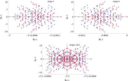
Figure S1: Complex eigenvalues of the Liouvillian belonging to the stripes 0, 3 and 1&2 for $\Gamma=8000$. Approximated eigenvalues (open red circles) are computed at order $1/\Gamma$ by Eqs. (S25) and (S26) for stripe 0, Eqs. (S35) and (S43) for stripe 3 and Eqs. (S56), (S57) and (S74) for stripes 1&2, and compare very well with the exact numerical results (blue dots). Parameters as in Fig. 1.

In the top right panel of Fig. S1, we compare the Liouvillian eigenvalues of this stripe evaluated numerically with those obtained by the above perturbative formulas. As expected according to Fig. 2, for the chosen value $\Gamma=8000$ we have an excellent agreement between the two sets of data.

Appendix G The $XYZ$ spin chain: corrections $O(1/\Gamma)$ for the spectrum associated to the nondegenerate dissipator eigenvalue $c_{3}=-1$

First of all, we note that for the $XYZ$ spin chain with dissipation at site 0 the operators $g_{k}=\mathop{\mathrm{tr}_{\mathcal{H}_{0}}}\limits((\psi_{k}\otimes I_{\mathcal{H}_{1}})H)$ are given by 2018ZenoDynamicsSM, Eqs. (41) and (42),

$$g_{1}=\left(\hat{J}(\vec{n}_{0}^{\prime}-i\vec{n}_{0})\right)\cdot\vec{\sigma}_{1},$$

$$g_{2}=g_{1}^{\dagger},$$

$$g_{3}=\left(\hat{J}\vec{n}_{0}\right)\cdot\vec{\sigma}_{1}.$$

The $O(1/\Gamma)$ corrections $\delta\lambda_{3,\alpha,\beta}$ to the Liouvillian eigenvalues $\lambda_{3,\alpha,\beta}=c_{3}\Gamma+i(\epsilon_{\alpha}-\epsilon_{\beta})$ are obtained from the second order of Dyson expansion and correspond to the terms $O(1/\Gamma)$ of Eq. (Full Spectrum of the Liouvillian of Open Dissipative Quantum Systems in the Zeno Limit). By explicitly calculating the coefficients $\gamma^{nsk}_{mz}$, $\epsilon^{nsk}_{zm}$ and $\delta^{nsk}_{zm}$ with $s=k=3$ and $n=0,1,2$, we find

$$\frac{d{R_{3}}}{d\tau} =\Gamma c_{3}R_{3}+i(U_{3}R_{3}-R_{3}W_{3})+\frac{1}{\Gamma}\left((1+\mu)E_{2,1}[R_{3}]+(1-\mu)E_{1,2}[R_{3}]-\frac{1-\mu^{2}}{2}{\cal D}_{g_{3}}[R_{3}]\right),$$ (S27)

where

$$U_{3} =V_{3}=g_{0}-\mu\ g_{3}^{\dagger}=\sum_{k=1}^{N-1}h_{k,k+1}-\mu(J\vec{n}_{0})\cdot\vec{\sigma}_{1},$$ (S28)

$$E_{n,m}[X] =g_{n}^{\dagger}g_{n}X+Xg_{n}^{\dagger}g_{n}+2g_{m}Xg_{m}^{\dagger},$$ (S29)

$${\cal D}_{g}[X] =gXg^{\dagger}-\frac{1}{2}g^{\dagger}gX-\frac{1}{2}Xg^{\dagger}g.$$ (S30)

For $\Gamma$ large, the last term in Eq. (S27) can be treated as a perturbation $V_{3}[R_{3}]$ of order $1/\Gamma$. The $O(1/\Gamma)$ corrections to the Liouvillian eigenvalues are then obtained via the standard perturbative formula $\delta\lambda_{3,\alpha,\beta}=\langle\alpha\beta|\hat{V}_{3}|\alpha\beta\rangle$, where $\hat{V}_{3}$ is the vectorized superoperator acting on the vectorized reduced density matrix $|R_{3}\rangle=|\alpha,\beta\rangle=|\alpha\rangle\otimes|\beta\rangle^{*}$ defined by $\hat{V}_{3}|R_{3}\rangle=V_{3}[R_{3}]$. We recall that $|\alpha\rangle$ and $|\beta\rangle$ are the eigenvectors of $V_{3}=V_{3}$,

$$U_{3}|\alpha\rangle=\epsilon_{\alpha}|\alpha\rangle.$$ (S31)

Note that $U_{3}$ is Hermitian and its eigenvalues $\epsilon_{\alpha}$ are real.

To explicitly illustrate the evaluation of $\delta\lambda_{3,\alpha,\beta}$, let’s start considering the simplest case $\mu=1$. By making the substitution $R_{3}(\tau)=e^{c_{3}\Gamma\tau}r_{3}(\tau)$, we obtain

$$\frac{d{r_{3}}}{d\tau} =i(U_{3}r_{3}-r_{3}U_{3})+\frac{2}{\Gamma}\left(g_{2}^{\dagger}g_{2}r_{3}+r_{3}g_{2}^{\dagger}g_{2}+2g_{1}r_{3}g_{1}^{\dagger}\right)$$

$$={\cal L}_{3}^{(0)}[r_{3}]+V_{3}[r_{3}].$$ (S32)

In the Zeno limit $\Gamma\rightarrow\infty$, Eq. (S32) for $r_{3}$ is linearized in terms of modes $|\alpha\rangle\langle\beta|$. In fact, $U_{3}$ can be obtained from $h_{D}$ by flipping the boundary term, therefore $h_{D}$ and $U_{3}$ are equivalent and have the same set of eigenvalues $\epsilon_{\alpha}$. It follows that, in an equivalent representation, the solution of the eigenvalue problem for the Liouvillian $\mathcal{L}^{(0)}_{3}[\cdot]$, namely, $\mathcal{L}^{(0)}_{3}[\psi_{j}]=\Lambda_{j}\psi_{j}$, is given by $\psi_{j}=|\alpha\rangle\langle\beta|$ and $\Lambda_{j}=i(\epsilon_{\alpha}-\epsilon_{\beta})$.

The expectation of an arbitrary superoperator of the form $V[r_{3}]=Qr_{3}W$ on the state $\psi_{j}=|\alpha\rangle\langle\beta|$ can be calculated in a vectorized form as

$$\langle\psi_{j}|\hat{V}|\psi_{j}\rangle=\langle\alpha|\otimes\langle\beta|^{*}(Q\otimes W^{t})|\alpha\rangle\otimes|\beta\rangle^{*}=\langle\alpha|Q|\alpha\rangle\langle\beta|^{*}W^{t}|\beta\rangle^{*}=\langle\alpha|Q|\alpha\rangle\langle\beta|W|\beta\rangle.$$ (S33)

It follows that, accounting for the corrections $O(1/\Gamma)$, for $\mu=1$ we obtain

$$\lambda_{3,\alpha,\beta} =c_{3}\Gamma+i(\epsilon_{\alpha}-\epsilon_{\beta})+\langle\psi_{j}|\hat{V}_{3}|\psi_{j}\rangle$$

$$=-\Gamma+i(\epsilon_{\alpha}-\epsilon_{\beta})+\frac{2}{\Gamma}\left(\langle\alpha|g_{2}^{\dagger}g_{2}|\alpha\rangle+\langle\beta|g_{2}^{\dagger}g_{2}|\beta\rangle+2\langle\alpha|g_{1}|\alpha\rangle\langle\beta|g_{1}^{\dagger}|\beta\rangle\right).$$ (S34)

This result is immediately generalised to arbitrary $\mu$

$$\lambda_{3,\alpha,\beta}= \ -\Gamma+i(\epsilon_{\alpha}-\epsilon_{\beta})$$

$$+\frac{1}{\Gamma}\left((1+\mu)\left(\langle\alpha|g_{2}^{\dagger}g_{2}|\alpha\rangle+\langle\beta|g_{2}^{\dagger}g_{2}|\beta\rangle+2\langle\alpha|g_{1}|\alpha\rangle\langle\beta|g_{1}^{\dagger}|\beta\rangle\right)\right.$$

$$\qquad+(1-\mu)\left(\langle\alpha|g_{1}^{\dagger}g_{1}|\alpha\rangle+\langle\beta|g_{1}^{\dagger}g_{1}|\beta\rangle+2\langle\alpha|g_{2}|\alpha\rangle\langle\beta|g_{2}^{\dagger}|\beta\rangle\right)$$

$$\qquad+\frac{1-\mu^{2}}{4}\left.\left(\langle\alpha|g_{3}^{\dagger}g_{3}|\alpha\rangle+\langle\beta|g_{3}^{\dagger}g_{3}|\beta\rangle-2\langle\alpha|g_{3}|\alpha\rangle\langle\beta|g_{3}^{\dagger}|\beta\rangle\right)\right).$$ (S35)

The above perturbative formula can be applied only if the unperturbed eigenvalue is nondegenerate. For $O(1)$ degenerate eigenvalues, $\lambda_{3,\alpha,\alpha}=-\Gamma$, the $O(1/\Gamma)$ corrections must be found in a different way. In the Zeno limit, we have a stationary solution $r_{3}(\infty)=\sum_{\alpha}\nu_{\alpha}|\alpha\rangle\langle\alpha|$. Taking into account the $O(1/\Gamma)$ terms, we can assume the finite-time $r_{3}(\tau)$ to have the same form but with coefficients $\nu_{\alpha}$ which depend on time, $r_{3}(\tau)=\sum_{\alpha}\nu_{\alpha}(\tau)|\alpha\rangle\langle\alpha|$. Then, from Eq. (S32) we have, for $\mu=1$,

$$\frac{d{\nu_{\alpha}}}{d\tau}=\frac{2}{\Gamma}\sum_{\beta}T_{\alpha,\beta}\nu_{\beta},$$ (S36)

where

$$T_{\alpha,\beta}=2w_{1,\alpha,\beta},\quad\beta\neq\alpha,\qquad T_{\alpha,\alpha}=2\sum_{\beta}w_{2,\beta,\alpha}+2w_{1,\alpha,\alpha},$$ (S37)

with

$$w_{n,\alpha,\beta} =\left|\langle\alpha|g_{n}|\beta\rangle\right|^{2}.$$ (S38)

For arbitrary values of $\mu$ we have, instead,

$$T_{\alpha,\beta}=w_{\alpha,\beta}(\mu),\quad\beta\neq\alpha,\qquad T_{\alpha,\alpha}=\sum_{\beta}f_{\beta,\alpha}(\mu)+w_{\alpha,\alpha}(\mu),$$ (S39)

with

$$w_{\alpha,\beta}(\mu) =(1+\mu)w_{1,\alpha,\beta}+(1-\mu)w_{2,\alpha,\beta}-\frac{1-\mu^{2}}{4}w_{3,\alpha,\beta},$$ (S40)

$$f_{\beta,\alpha}(\mu) =(1+\mu)w_{2,\beta,\alpha}+(1-\mu)w_{1,\beta,\alpha}+\frac{1-\mu^{2}}{4}w_{3,\beta,\alpha}.$$ (S41)

By finding the eigenvalues $\mu_{\alpha}$ of the matrix $T$, we resolve the degeneracy problem. In fact, in terms of the corresponding eigenvectors $\tilde{\nu}_{\alpha}$ of $T$, we have

$$\frac{d{\tilde{\nu}_{\alpha}}}{d\tau}=\frac{2}{\Gamma}\mu_{\alpha}\tilde{\nu}_{\alpha},$$ (S42)

the set of the values $(2/\Gamma)\mu_{\alpha}$ being the $1/\Gamma$ correction to the set of the degenerate eigenvalues $\lambda_{3,\alpha,\alpha}$,

$$\lambda_{3,\alpha,\alpha}=-\Gamma+\frac{2}{\Gamma}\mu_{\alpha},\qquad\alpha=1,2,\dots,2^{N}.$$ (S43)

Numerically, for the integrable $XYZ$ model, we find the matrix $T$ to be equivalent to a symmetric real matrix, so that all its eigenvalues $\mu_{\alpha}$ are real. Since $c_{3}=-1$ is real too, the eigenvalues (S43) lie on the real axis.

Appendix H The $XYZ$ spin chain: spectrum associated to the degenerate dissipator eigenvalue $c_{1}=c_{2}=-1/2$

Equation (Full Spectrum of the Liouvillian of Open Dissipative Quantum Systems in the Zeno Limit) for $k=1,2$ has the form

$$\frac{dR_{k}}{d\tau}= \ \Gamma c_{1}R_{k}+i\sum_{s=1}^{2}\left(U_{k,s}R_{s}-R_{s}W_{k,s}\right)$$

$$+\frac{1}{\Gamma}\sum_{z>0}\sum_{m>0}\sum_{n=0,3}\sum_{s=1}^{2}\frac{1}{c_{n}-c_{1}}\left(-\gamma^{n,s,k}_{m,z}g_{m}R_{s}g_{z}^{\dagger}+\epsilon^{n,s,k}_{z,m}g_{z}^{\dagger}g_{m}R_{s}+\delta^{n,s,k}_{z,m}R_{s}g_{z}^{\dagger}g_{m}\right)$$

$$= \ \Gamma c_{1}R_{k}+i\sum_{s=1}^{2}\left(U_{k,s}R_{s}-R_{s}W_{k,s}\right)$$

$$+\frac{2}{\Gamma}\sum_{z>0}\sum_{m>0}\sum_{s=1}^{2}\left(-\tilde{\gamma}^{s,k}_{m,z}g_{m}R_{s}g_{z}^{\dagger}+\tilde{\epsilon}^{s,k}_{z,m}g_{z}^{\dagger}g_{m}R_{s}+\tilde{\delta}^{s,k}_{z,m}R_{s}g_{z}^{\dagger}g_{m}\right),$$ (S44)

where

$$\tilde{\gamma}^{s,k}_{m,z} =\gamma^{0,s,k}_{m,z}-\gamma^{3,s,k}_{m,z},$$ (S45)

$$\tilde{\epsilon}^{s,k}_{m,z} =\epsilon^{0,s,k}_{m,z}-\epsilon^{3,s,k}_{m,z},$$ (S46)

$$\tilde{\delta}^{s,k}_{m,z} =\delta^{0,s,k}_{m,z}-\delta^{3,s,k}_{m,z},$$ (S47)

with

$$\gamma^{n,s,k}_{m,z} =C_{m,s,n}A_{z,n,k}+A_{z,s,n}C_{m,n,k},$$ (S48)

$$\epsilon^{n,s,k}_{z,m} =C_{m,s,n}B_{z,n,k},$$ (S49)

$$\delta^{n,s,k}_{z,m} =A_{z,s,n}C_{k,n,m}.$$ (S50)

The only nonzero coefficients $\tilde{\gamma}^{s,k}_{m,z}$, $\tilde{\epsilon}^{s,k}_{m,z}$ and $\tilde{\delta}^{s,k}_{m,z}$ are

$$\tilde{\gamma}^{1,1}_{1,1} =\tilde{\gamma}^{2,2}_{1,1}=1+\mu,$$

$$\tilde{\gamma}^{1,1}_{2,2} =\tilde{\gamma}^{2,2}_{2,2}=1-\mu,$$

$$\tilde{\epsilon}^{2,2}_{2,2} =-\tilde{\epsilon}^{1,1}_{1,1}=\mu,$$

$$\tilde{\epsilon}^{2,1}_{1,2} =1-\mu,\qquad\tilde{\epsilon}^{1,2}_{2,1}=1+\mu,$$

$$\tilde{\delta}^{1,1}_{2,2} =-\tilde{\epsilon}^{2,2}_{1,1}=\mu,$$

$$\tilde{\delta}^{2,1}_{1,2} =1+\mu,\qquad\tilde{\delta}^{1,2}_{2,1}=1-\mu.$$

After the substitution $R_{1}(\tau)=e^{c_{1}\Gamma\tau}r_{1}(\tau)$ and $R_{2}(\tau)=e^{c_{1}\Gamma\tau}r_{2}(\tau)$, we obtain the following equations of motion for $r_{1}(\tau)$ and $r_{2}(\tau)$.

$$\frac{d{r_{1}}}{d\tau}= \ i\left(f_{+}r_{1}-r_{1}f_{-}\right)$$

$$+\frac{2}{\Gamma}\left(-(1+\mu)g_{1}r_{1}g_{1}^{\dagger}-(1-\mu)g_{2}r_{1}g_{2}^{\dagger}-\mu g_{1}^{\dagger}g_{1}r_{1}+\mu r_{1}g_{2}^{\dagger}g_{2}+\right.$$

$$\qquad\left.+(1-\mu)g_{1}^{\dagger}g_{2}r_{2}+(1+\mu)r_{2}g_{1}^{\dagger}g_{2}\right),$$ (S51)

$$\frac{d{r_{2}}}{d\tau}= \ i\left(f_{-}r_{2}-r_{2}f_{+}\right)$$

$$+\frac{2}{\Gamma}\left(-(1+\mu)g_{1}r_{2}g_{1}^{\dagger}-(1-\mu)g_{2}r_{2}g_{2}^{\dagger}+\mu g_{2}^{\dagger}g_{2}r_{2}-\mu r_{2}g_{1}^{\dagger}g_{1}+\right.$$

$$\qquad\left.+(1+\mu)g_{2}^{\dagger}g_{1}r_{1}+(1-\mu)r_{1}g_{2}^{\dagger}g_{1}\right),$$ (S52)

where, we recall that $g_{0}=h_{D}$,

$$f_{\pm}=g_{0}\pm\frac{1\mp\mu}{2}g_{3}^{\dagger}=\sum_{j=1}^{N-1}h_{j,j+1}\pm(J\vec{n}_{0})\cdot\vec{\sigma}_{1}.$$ (S53)

At zeroth order in $1/\Gamma$, the eigenmodes of Eqs. (S51) and (S52) are, respectively, $|\alpha\rangle\langle\tilde{\beta}|$ and $|\tilde{\alpha}\rangle\langle\beta|$, where $|\alpha\rangle$ and $|\tilde{\alpha}\rangle$ are the eigenvectors of $f_{+}$ and $f_{-}$, namely, $f_{+}|\alpha\rangle=\epsilon_{\alpha}|\alpha\rangle$ and $f_{-}|\tilde{\alpha}\rangle=\epsilon_{\alpha}|\tilde{\alpha}\rangle$. Note that $f_{+}$ and $f_{-}$, being related by a unitary transformation, have the same eigenvalues. It follows that the zeroth order eigenvalues of the Liouvillian are twice degenerate,

$$\lambda_{1,\alpha,\beta}=-\frac{\Gamma}{2}+i(\epsilon_{\alpha}-\epsilon_{\beta})+O(1/\Gamma),$$ (S54)

$$\lambda_{2,\alpha,\beta}=\lambda_{1,\alpha,\beta}+O(1/\Gamma),$$ (S55)

the respective eigenvectors being $r_{1}^{(0)}=|\alpha\rangle\langle\tilde{\beta}|$ and $r_{2}^{(0)}=|\tilde{\alpha}\rangle\langle\beta|$. Note that the zeroth-order eigenvalues $\lambda_{1,\alpha,\beta}$ and $\lambda_{2,\alpha,\beta}$ have a double degeneracy for $\alpha\neq\beta$ and a degeneracy $2^{N+1}$ for $\alpha=\beta$.

To obtain the $O(1/\Gamma)$ corrections to the degenerate eigenvalues $\lambda_{1,\alpha,\beta}=\lambda_{2,\alpha,\beta}=-\Gamma/2+i(\epsilon_{\alpha}-\epsilon_{\beta})\equiv\Lambda_{\alpha\beta}$, we substitute the Ansatz $r_{1}(\tau)=x_{1}(\tau)|\alpha\rangle\langle\tilde{\beta}|$ and $r_{2}(\tau)=x_{2}(\tau)|\tilde{\alpha}\rangle\langle\beta|$ into Eqs. (S51) and (S52), obtaining the following equations for $x_{1}(\tau)$ and $x_{2}(\tau)$

$$\frac{dx_{1}}{d\tau}= \ \Lambda_{\alpha\beta}x_{1}+\frac{2}{\Gamma}(V_{11}x_{1}+V_{12}x_{2}),$$

$$\frac{dx_{2}}{d\tau}= \ \Lambda_{\alpha\beta}x_{2}+\frac{2}{\Gamma}(V_{21}x_{1}+V_{22}x_{2}),$$

where

$$V_{11} =-(1+\mu)\langle\alpha|g_{1}|\alpha\rangle\langle\tilde{\beta}|g_{1}^{\dagger}|\tilde{\beta}\rangle-(1-\mu)\langle\alpha|g_{2}|\alpha\rangle\langle\tilde{\beta}|g_{2}^{\dagger}|\tilde{\beta}\rangle-\mu\langle\alpha|g_{1}^{\dagger}g_{1}|\alpha\rangle+\mu\langle\tilde{\beta}|g_{2}^{\dagger}g_{2}|\tilde{\beta}\rangle,$$

$$V_{22} =-(1+\mu)\langle\tilde{\alpha}|g_{1}|\tilde{\alpha}\rangle\langle\beta|g_{1}^{\dagger}|\beta\rangle-(1-\mu)\langle\tilde{\alpha}|g_{2}|\tilde{\alpha}\rangle\langle\beta|g_{2}^{\dagger}|\beta\rangle+\mu\langle\tilde{\alpha}|g_{2}^{\dagger}g_{2}|\tilde{\alpha}\rangle-\mu\langle\beta|g_{1}^{\dagger}g_{1}|\beta\rangle,$$

$$V_{12} =(1+\mu)\langle\alpha|\tilde{\alpha}\rangle\langle\beta|g_{1}^{\dagger}g_{2}|\tilde{\beta}\rangle+(1-\mu)\langle\alpha|g_{1}^{\dagger}g_{2}|\tilde{\alpha}\rangle\langle\beta|\tilde{\beta}\rangle,$$

$$V_{21} =(1+\mu)\langle\tilde{\alpha}|g_{2}^{\dagger}g_{1}|\alpha\rangle\langle\tilde{\beta}|\beta\rangle+(1-\mu)\langle\tilde{\alpha}|\alpha\rangle\langle\tilde{\beta}|g_{2}^{\dagger}g_{1}|\beta\rangle.$$

The eigenvalues $v_{1},v_{2}$ of the matrix $V$ with elements $V_{ij}$ give the corrections to the eigenvalues $-\Gamma/2+i(\epsilon_{\alpha}-\epsilon_{\beta})$,

$$\lambda_{1\alpha\beta} =-\Gamma/2+i(\epsilon_{\alpha}-\epsilon_{\beta})+\frac{2}{\Gamma}v_{1},$$ (S56)

$$\lambda_{2\alpha\beta} =-\Gamma/2+i(\epsilon_{\alpha}-\epsilon_{\beta})+\frac{2}{\Gamma}v_{2}.$$ (S57)

For degenerate eigenvalues $\lambda_{1,\alpha,\alpha}=\lambda_{2,\alpha,\alpha}=-\Gamma/2$, the $O(1/\Gamma)$ corrections have to be calculated in the following way. In the Zeno limit, the stationary solutions of Eqs. (S51) and (S52) are, respectively, $r_{1}(\infty)=\sum_{\alpha}\nu_{\alpha}|\alpha\rangle\langle\tilde{\alpha}|$ and $r_{2}(\infty)=\sum_{\alpha}\mu_{\alpha}|\tilde{\alpha}\rangle\langle\alpha|$. Therefore, for $r_{1}(\tau)$ and $r_{2}(\tau)$ we may assume the form $r_{1}(\tau)=\sum_{\alpha}\nu_{\alpha}(\tau)|\alpha\rangle\langle\tilde{\alpha}|$ and $r_{2}(\tau)=\sum_{\alpha}\mu_{\alpha}(\tau)|\tilde{\alpha}\rangle\langle\alpha|$ with coefficients $\nu_{\alpha}$ and $\mu_{\alpha}$ depending on time. Inserting these expressions into Eqs. (S51) and (S52) and writing down the equations for the components $\langle\alpha|r_{1}(\tau)|\tilde{\alpha}\rangle=\nu_{\alpha}(\tau)$ and $\langle\tilde{\alpha}|r_{2}(\tau)|\alpha\rangle=\mu_{\alpha}(\tau)$, we have

$$\frac{d{\nu_{\alpha}}}{d\tau} =\frac{2}{\Gamma}\sum_{\beta}\left(T^{11}_{\alpha\beta}\nu_{\beta}+T^{12}_{\alpha\beta}\mu_{\beta}\right),$$ (S58)

$$\frac{\partial{\mu_{\alpha}}}{\partial\tau} =\frac{2}{\Gamma}\sum_{\beta}\left(T^{21}_{\alpha\beta}\nu_{\beta}+T^{22}_{\alpha\beta}\mu_{\beta}\right),$$ (S59)

where

$$T^{11}_{\alpha\beta} =w_{1}(\alpha,\beta),\qquad\beta\neq\alpha,$$ (S60)

$$T^{22}_{\alpha\beta} =w_{2}(\alpha,\beta),\qquad\beta\neq\alpha,$$ (S61)

$$T^{12}_{\alpha\beta} =w_{12}(\alpha,\beta),$$ (S62)

$$T^{21}_{\alpha\beta} =w_{21}(\alpha,\beta),$$ (S63)

$$T^{11}_{\alpha\alpha} =w_{1}(\alpha,\alpha)+\sum_{\beta}f(\alpha,\beta),$$ (S64)

$$T^{22}_{\alpha\alpha} =w_{2}(\alpha,\alpha)+\sum_{\beta}f(\alpha,\beta),$$ (S65)

and

$$w_{1}(\alpha,\beta) =-(1+\mu)\langle\alpha|g_{1}|\beta\rangle\langle\tilde{\beta}|g_{1}^{\dagger}|\tilde{\alpha}\rangle-(1-\mu)\langle\alpha|g_{2}|\beta\rangle\langle\tilde{\beta}|g_{2}^{\dagger}|\tilde{\alpha}\rangle,$$ (S66)

$$w_{2}(\alpha,\beta) =-(1+\mu)\langle\tilde{\alpha}|g_{1}|\tilde{\beta}\rangle\langle\beta|g_{1}^{\dagger}|\alpha\rangle-(1-\mu)\langle\tilde{\alpha}|g_{2}|\tilde{\beta}\rangle\langle\beta|g_{2}^{\dagger}|\alpha\rangle,$$ (S67)

$$f(\alpha,\beta) =\mu|\langle\tilde{\beta}|g_{2}|\tilde{\alpha}\rangle|^{2}-\mu|\langle\beta|g_{1}|\alpha\rangle|^{2},$$ (S68)

$$w_{12}(\alpha,\beta) =(1-\mu)\langle\alpha|\tilde{\beta}\rangle\langle\beta|g_{1}^{\dagger}g_{2}|\tilde{\alpha}\rangle+(1+\mu)\langle\beta|\tilde{\alpha}\rangle\langle\alpha|g_{1}^{\dagger}g_{2}|\tilde{\beta}\rangle,$$ (S69)

$$w_{21}(\alpha,\beta) =(1-\mu)\langle\tilde{\alpha}|\beta\rangle\langle\tilde{\beta}|g_{2}^{\dagger}g_{1}|\alpha\rangle+(1+\mu)\langle\tilde{\beta}|\alpha\rangle\langle\tilde{\alpha}|g_{2}^{\dagger}g_{1}|\beta\rangle.$$ (S70)

By finding the eigenvalues $q_{\alpha}$ of the block matrix

$$T=\left(\begin{array}[]{cc}T^{11}&T^{12}\\ T^{21}&T^{22}\end{array}\right),$$ (S73)

we resolve the degeneracy problem. The real eigenvalues with $O(1/\Gamma)$ corrections, belonging to the degenerate eigenvalue $c_{1}=c_{2}$ of the dissipator, are given by

$$\lambda_{1\&2,\alpha,\alpha}=\frac{\Gamma}{2}+\frac{2}{\Gamma}q_{\alpha},\qquad\alpha=1,2,\dots,2\times 2^{N}.$$ (S74)

Numerically, we find that all the coefficients of the matrix $T$, as the operators $f_{\pm}$, are $\mu$ independent and, therefore, the corrections $q_{\alpha}$ in Eq. (S74) are $\mu$ independent. This property is exceptional and probably connected with the integrability of the $XYZ$ model.

Appendix I Properties of the auxiliary Markov Matrix $M_{ab}$

It is well known that the eigenvalues of a generic stochastic matrix are complex. Nevertheless, for our case example – the XYZ model with Zeno boundary dissipation – all the eigenvalues happen to be real.

Here we prove this exceptional property, namely, that the eigenvalues $\mu_{a}$ of the Markov matrix $M_{ab}$ in Eq (S26) are all real, for pure state boundary driving $\mu=1$. We observe (numerically) that the elements $M_{ab}$ of the Matrix Markov process,

$$\frac{d\nu_{\alpha}(\tau)}{d\tau}=\frac{1}{\Gamma}\sum_{\beta}M_{\alpha\beta}\ \nu_{\beta}(\tau),$$ (S75)

satisfy the so-called Kolmogorov condition

$$M_{ab}M_{bc}M_{ca}=M_{ac}M_{cb}M_{ba},$$ (S76)

with $a,b,c$ arbitrary and all different, if the targeted state at the boundary is pure, i.e., for $\mu=1$. The Kolmogorov condition and the positivity of the non-diagonal elements $M_{ab}$ entail

$$M_{ab}=s(a,b)\pi_{b},$$

$$s(a,b)=s(b,a),$$

with $s(a,b)$ and $\pi_{b}$ real and positive. Introducing the diagonal matrix $\hat{\pi}$ with elements $\pi_{a}$, we can write the Markov matrix $M$ as

$$M=\hat{\pi}S,$$

where $S$ is the matrix with non-diagonal elements $S_{ab}=s(a,b)$ and $S_{aa}=M_{aa}/{\pi_{a}}$. The above relation can be rewritten as

$$\hat{\pi}^{-1/2}M\hat{\pi}^{1/2}=\hat{\pi}^{1/2}S\hat{\pi}^{1/2}.$$

Obviously, the RHS of the above equation is a real symmetric matrix, since $S$ is a real symmetric matrix. Consequently, $\hat{\pi}^{-1/2}M\hat{\pi}^{1/2}$ is also a real symmetric matrix, i.e., the Markov matrix $M$ is equivalent to a real symmetric matrix. Therefore, the eigenvalues $\mu_{a}$ of $M$ are all real. It follows that the $2^{N}$ Liouvillian eigenvalues belonging to the first stripe (S26) lie, in the Zeno limit, on the real axis.

The same argument can be repeated for all stripes, and consequently, all the Liouvillian eigenvalues of type $\lambda_{k,\alpha,\alpha}$ are, near the Zeno limit, real. In total, for our $XYZ$ spin chain, there are $4\times 2^{N}=2^{N+2}$ real Liouvillian eigenvalues, while all the remaining Liouvillian eigenvalues $\lambda_{k,\alpha,\beta}$, with $\alpha\neq\beta$ generically, i.e., in the absence of extra degeneracies, have a nonzero imaginary part.

Finally, for $\mu\neq 1$ we observe numerically the same situation, i.e., the eigenvalues of the Markov matrix $M$ (and its analogs for the other stripes) are all real, so that the Zeno-limit Liouvillian spectrum contains $2^{N+2}$ real entries. Clearly, also in this case $M$ must be equivalent to a Hermitian matrix. However, this fact can no longer be explained by the Kolmogorov property (S76), (equivalent to a detailed balance condition for the Markov rates $w_{ab}=M_{ba}$) since this property is violated for $\mu\neq\pm 1$, and the detailed balance condition $\pi_{a}w_{ab}=\pi_{b}w_{ba}$ is consequently not satisfied. Further studies are required to clarify this subtle issue.

Appendix J Zeno limit for a problem with two qubits

Consider a problem (1) with $H=\vec{\sigma}_{0}\cdot(\hat{J}\vec{\sigma}_{1})$, where $\hat{J}=\mathrm{diag}(J_{x},J_{y},J_{z})\equiv\mathrm{diag}(1,\gamma,\Delta)$, and

$$\mathcal{D}[\rho]=\sigma_{0}^{+}\rho\sigma_{0}^{-}-\frac{1}{2}\sigma_{0}^{-}\sigma_{0}^{+}\rho-\frac{1}{2}\rho\sigma_{0}^{-}\sigma_{0}^{+}.$$ (S77)

According to our general theory, the stripe closest to the imaginary axis, in the Zeno limit contains $4$ eigenvalues. They are governed by the effective Hamiltonian (S24)

$$h_{D}=\Delta\ \sigma^{z}$$ (S78)

and by the effective Lindblad operator

$$\tilde{L}_{1}=-\left(\begin{array}[]{cc}0&1+\gamma\\ 1-\gamma&0\end{array}\right).$$ (S81)

The near-Zeno limit eigenvalues for the first stripe are given by Eq. (S25),

$$\lambda_{0,1,1}=0,$$

$$\lambda_{0,1,2}=-4\frac{1+\gamma^{2}}{\Gamma}-2\Delta i,$$

$$\lambda_{0,2,1}=\lambda_{0,1,2}^{*},$$

$$\lambda_{0,2,2}=-8\frac{1+\gamma^{2}}{\Gamma}.$$

Analogously, we obtain the other Liouvillian eigenvalues. The full set of $16$ Liouvillian eigenvalues $\lambda$ up to order $1/\Gamma$ is given by

$$\lambda_{0,\alpha,\beta}=\left\{0,-2\frac{\gamma_{+}}{\Gamma},-\frac{\gamma_{+}}{\Gamma}\pm 2\Delta i\right\},$$

$$\lambda_{1\&2,\alpha,\beta}=\left\{-\frac{\Gamma}{2},-\frac{\Gamma}{2},-\frac{\Gamma}{2}\pm\frac{2\gamma_{-}}{\Gamma},-\frac{\Gamma}{2}\pm\frac{8\gamma}{\Gamma}\pm 2\Delta i\right\},$$ (S82)

$$\lambda_{3,\alpha,\beta}=\left\{-\Gamma,-\Gamma+2\frac{\gamma_{+}}{\Gamma},-\Gamma+\frac{\gamma_{+}}{\Gamma}\pm 2\Delta i,\right\},$$

where $\gamma_{\pm}=4(1\pm\gamma^{2})$. The respective eigenfunctions are fully analytic functions of $\Gamma$ in the Zeno regime ($\Gamma>\Gamma_{\mathrm{cr}}$, see later for its definition) so the Liouvillian is diagonalizable in any point. In the following considerations, the free fermion point $\Delta=0$ must be excluded, since it corresponds to zero $h_{D}$ and multiple degeneracies even in the Zeno limit (S82).

As discussed in the main text, the analyticity of Liouvillian eigenvalues breaks down at the branch points, which can be located by finding the eigenvalues of the Liouvillian for arbitrary $\Gamma,\gamma,\Delta$. An inspection shows that among the 16 eigenvalues for $\Delta\neq 0$, apart from $\lambda=0$ there is a double degenerate real eigenvalue $\lambda=-\Gamma/2$, the eigenvalue $\lambda=-\Gamma$ and all the other eigenvalues contain branch points. Depending on the parameters, there can be up to $8$ values of $\Gamma=\Gamma_{i}$ where branchings occur. Two points are $\Gamma_{1}=8$ and $\Gamma_{2}=8|\gamma|$, while the location of the other branch points $\Gamma_{3},\dots,\Gamma_{8}$ involves radicals of a quartic equation. In particular, for small $\Delta$ we find a singularity, for $\max(\Gamma_{3},\ldots\Gamma_{8})=O(1/|\Delta|)$, which has a probable origin in the repulsion of the eigenvalues, which, for $|\Delta|\ll 1$, become too close each other. The onset of the fully analytic Zeno regime sets in beyond the rightmost branching points, i.e., for $\Gamma>\Gamma_{\mathrm{cr}}\equiv\max_{i}{\Gamma_{i}}$. The value of $\Gamma_{\mathrm{cr}}$ is easily estimated numerically for a generic choice of the model parameters, see Fig. 3 for an example.

References

(1) V. Kendon, Quantum computing using
continuous-time evolution, Interface Focus 10, 20190143
(2020).
(2) J. Cao et al., Quantum biology revisited,
Science Advances 6, eaaz4888 (2020).
(3) H.-J. Briegel and B.-G. Englert Quantum
optical master equations: The use of damping bases, Phys. Rev. A
47, 3311 (1993).
(4) S. M. Barnett and S. Stenholm Spectral
decomposition of the Lindblad operator Journal of Modern Optics,
47, 2869-2882 (2000).
(5) D. Rocca, R. Gebauer, Y. Saad, and S. Baroni,
Turbo charging time-dependent density-functional theory with Lanczos
chains, The Journal of Chemical Physics 128, 154105 (2008).
(6) J. M. Torres, R. Betzholz,
M. Bienert Optomechanical damping basis, J. Phys. A:
Math. Theor. 52, 08LT02 (2019).
(7) M. Marcuzzi, J. Schick, B. Olmos, and
I. Lesanovsky, Effective dynamics of strongly dissipative Rydberg
gases, J. Phys. A: Math. Theor. 47, 482001 (2014).
(8) V. V. Albert, B. Bradlyn, M. Fraas, and
L. Jiang, Geometry and Response of Lindbladians, Phys. Rev. X
6, 041031 (2016).
(9) O. Shpielberg, Diffusion and entanglement in open
quantum systems, Europhysics Letters, 129, 60005 (2020).
(10) M. V. Medvedyeva, F. H. L. Essler, and T. Prosen, Exact
Bethe Ansatz Spectrum of a Tight-Binding Chain with Dephasing Noise,
Phys. Rev. Lett. 117, 137202 (2016).
(11) L. R. Bakker, V. I. Yashin, D. V. Kurlov,
A. K. Fedorov, and V. Gritsev, Lie-algebraic approach to
one-dimensional translationally invariant free-fermionic dissipative
systems, Phys. Rev. A 102, 052220 (2020).
(12) B. Buca, C. Booker, M. Medenjak, and D. Jaksch, Bethe
ansatz approach for dissipation: Exact solutions of quantum
many-body dynamics under loss, New J. Phys. 22, 123040
(2020).
(13) M. Nakagawa, N. Kawakami, and M. Ueda, Exact Liouvillian
Spectrum of a One-Dimensional Dissipative Hubbard Model,
Phys. Rev. Lett. 126, 110404 (2021).
(14) B. Misra and E. C. G. Sudarshan, The Zeno’s
paradox in quantum theory, Journal of Mathematical Physics
18, 756 (1977).
(15) C. Presilla, R. Onofrio, and U. Tambini, Measurement
quantum mechanics and experiments on quantum Zeno effect,
Ann. Phys. (NY) 248, 95 (1996).
(16) K. Koshino and A. Shimizu,
Quantum Zeno effect by general measurements, Physics Reports
412, 191 (2005).
(17) D. Burgarth, P. Facchi, H. Nakazato, S.
Pascazio, and K. Yuasa, Quantum Zeno dynamics from general quantum
operations, Quantum, 4, 289 (2020).
(18) V. Popkov, S. Essink, C. Presilla, and
G. M. Schütz, Effective quantum Zeno dynamics in dissipative
quantum systems, Phys. Rev. A 98, 052110 (2018).
(19) P. Zanardi and L. Campos Venuti, Coherent Quantum
Dynamics in Steady-State Manifolds of Strongly Dissipative Systems,
Phys. Rev. Lett. 113, 240406 (2014).
(20) V. Gorini and A. Kossakowski, -level system in
contact with a singular reservoir, J. Math. Phys. 17, 1298
(1976).
(21) See Supplemental material at
http://link.aps.org/supplemental/10.1103/PhysRevLett.000.000000
(22) L. D. Landau and E. M. Lifshitz, Quantum
Mechanics: Non-Relativistic Theory, 3rd ed. (Pergamon Press,
Oxford, UK, 1989).
(23) T. Prosen, Exact nonequilibrium steady state of a
strongly driven open XXZ chain, Phys. Rev. Lett. 107,
137201 (2011).
(24) D. E. Evans, Irreducible quantum dynamical semigroups,
Commun. Math. Phys. 54, 293 (1977).
(25) V. Popkov, S. Essink, C. Kollath, and
C. Presilla, Dissipative generation of pure steady states and a
gambler’s ruin problem, Phys. Rev. A 102, 032205 (2020).
(26) T. Kato, Perturbation Theory of Linear
Operators (Springer, Berlin, 1966).
(27) E. J. Bergholtz, J. C. Budich, and F. K. Kunst,
Exceptional topology of non-Hermitian systems,
Rev. Mod. Phys. 93, 015005 (2021).
(28) W. D. Heiss, The physics of exceptional points,
J. Phys. A: Math. Theor. 45, 444016 (2012).
(29) N. Hatano, Exceptional points of the Lindblad
operator of a two-level system, Molecular Physics, 117,
2121-2127 (2019).
(30) K. Wang, F. Piazza, and
D. J. Luitz, Hierarchy of Relaxation Timescales in Local Random
Liouvillians, Phys. Rev. Lett. 124, 100604 (2020).
(31) V. Popkov, T. Prosen, L. Zadnik, Exact
Nonequilibrium Steady State of Open Spin-1/2 Chain with
Dirichlet Boundary Conditions, Phys. Rev. Lett. 124, 160403
(2020).
(32) V. Popkov, T. Prosen, L. Zadnik, Inhomogeneous
matrix product ansatz and exact steady states of boundary-driven
spin chains at large dissipation, Phys. Rev. E 101, 042122
(2020).
(33) B. Bertini, F Heidrich-Meisner,
C. Karrasch, T. Prosen, R. Steinigeweg, M. Znidaric,
Finite-temperature transport in one-dimensional quantum lattice
models, arXiv:2003.03334, Rev. Mod. Phys., Accepted 3 November 2020.
(34) Y. Wang, W.-L. Yang, J. Cao, and K. Shi,
Off-Diagonal Bethe Ansatz for Exactly Solvable Models,
(Springer, New York 2015) ISBN 978-3-662-46755-8.
(35) T. Can, V. Oganesyan,
D. Orgad, and S. Gopalakrishnan, Spectral Gaps and Midgap States in
Random Quantum Master Equations, Phys. Rev. Letters 123,
234103 (2019).