A Census of the Extended Neutral Hydrogen Around 18 MHONGOOSE Galaxies

Abstract

We present the analysis of the diffuse, low column density Hi environment of 18 MHONGOOSE galaxies. We obtained deep observations with the Robert C. Byrd Green Bank Telescope, and reached down to a $3\sigma$ column density detection limit of $N_{\rm HI}\,$$=6.3\times 10^{17}\,\rm cm^{-2}$ over a $20\,\rm km\,s^{-1}$ linewidth. We analyze the environment around these galaxies, with a focus on Hi gas that reaches column densities below $N_{\rm HI}\,$$=10^{19}\,\rm cm^{-2}$. We calculate the total amount of Hi gas in and around the galaxies revealing that nearly all of these galaxies contained excess Hi outside of their disks. We quantify the amount of diffuse gas in the maps of each galaxy, defined by Hi gas with column densities below $10^{19}\,\rm cm^{-2}$, and find a large spread in percentages of diffuse gas. However, by binning the percentage of diffuse Hi into quarters, we find that the bin with the largest number of galaxies is the lowest quartile ($0-25\%$ diffuse Hi ). We identified several galaxies which may be undergoing gas accretion onto the galaxy disk using multiple methods of analysis, including azimuthally averaging column densities beyond the disk, and identifying structure within our integrated intensity (Moment 0) maps. We measured Hi mass outside the disks of most of our galaxies, with rising cumulative flux even at large radii. We also find a strong correlation between the fraction of diffuse gas in a galaxy and its baryonic mass, and test this correlation using both Spearman and Pearson correlation coefficients. We see evidence of a dark matter halo mass threshold of $M_{halo}\sim 10^{11.1}$ $\rm M_{\sun}$ in which galaxies with high fractions of diffuse Hi all reside below. It is in this regime in which cold-mode accretion should dominate. Finally, we suggest a rotation velocity of $v_{rot}\sim 80\,\rm km\,s^{-1}$ as an upper threshold to find diffuse gas-dominated galaxies.

1 Introduction

The question of how galaxies get their gas and how they use this gas to continue to form stars remains among the main unanswered questions in astronomy. We know that as the star formation rate density over cosmic time has decreased since a redshift of z$\sim 2$ (Madau & Dickinson, 2014), the neutral hydrogen gas density has remained nearly constant since z$\sim 4$ (Rhee et al., 2018). Di Teodoro & Fraternali (2014) show that mergers of dwarf galaxies with spiral galaxies do not provide sufficient extra mass to sustain star formation in those galaxies. Even so, if star formation in spiral galaxies is not sustained by mergers alone, then they must be accreting the gas from the intergalactic medium (IGM).

Gas accreting from the IGM flows into the galaxy via diffuse filamentary structures (Birnboim & Dekel, 2003; Katz et al., 2003; Kereš et al., 2005). The gas travels from the cosmic web (Bond et al., 1996) through these filaments, and into the circumgalactic medium (CGM) of galaxies before falling onto the galaxy disk. The process of accretion described here typically proceeds via the hot or the cold mode (Kereš et al., 2005), where gas entering the halo either becomes shock heated to the virial temperature before cooling and condensing onto the galaxy disk or it flows along cold filaments through the CGM and remains cool as is falls onto the disk. While gas in both scenarios is predominantly ionized, the gas accreting via the cold-mode maintains a small neutral fraction, making detection feasible. Cold accretion dominates in the lower mass galaxy regime and favors low galaxy density environments. Observations of the CGM and disks of galaxies encompassing a range of these parameters will provide insight into cold accretion from the IGM and potentially direct detections of this gas falling onto galaxies.

Deep Hi surveys provide the observational link to direct detections of the effects of cold mode accretion from the IGM. The MeerKAT Hi Observations of Nearby Galactic Objects; Observing Southern Emitters (MHONGOOSE; de Blok et al. 2016) survey will provide high spatial resolution, high column density sensitivity maps of 30 nearby disk and dwarf galaxies. Most other Hi surveys achieve one or the other, but not both, with the exception of the IMAGINE survey with ATCA, which still has a much lower angular resolution than MHONGOOSE. HIPASS (Koribalski et al., 2004) and ALFALFA (Haynes et al., 2011) surveys provide an extremely large number of Hi detections, although neither at high resolution nor with column density sensitivities matching ours. High resolution surveys such as THINGS (Walter et al., 2008) and HALOGAS (Heald et al., 2011) (one of the first high resolution surveys designed to systematically detect accretion of Hi ), achieve column density sensitivities of $\sim 10^{20}\,\rm cm^{-2}$ and $\sim 10^{19}\,\rm cm^{-2}$, respectively. These levels of column densities enable detection of clumpy Hi that could be missed by a single dish telescope, yet would not be low enough to detect any extended or more diffuse gas accreting from the IGM. The MHONGOOSE survey will use the South African MeerKAT radio telescope, a 64-dish precursor to the Square Kilometre Array (SKA), to map these 30 galaxies to a $3\sigma$ column density detection limit of $7.5\times 10^{18}\,\rm cm^{-2}$ over a $16\,\rm km\,s^{-1}$ linewidth at an angular resolution of $30^{\prime\prime}$. At their poorest angular resolution, $90^{\prime\prime}$, this column density limit goes down to $5.5\times 10^{17}\,\rm cm^{-2}$. The high resolution maps produced by MHONGOOSE will further our understanding of how galaxies get their gas, how galaxies sustain star formation, and how matter that we can detect relates to the dark matter associated with galaxies, influencing galactic evolution. Specifically, this survey will help us to understand how gas flows in or out of galaxies, the conditions that allow the fuelling of star formation, accretion from the IGM, and ultimately its connection to the cosmic web (e.g. Carignan 2016). The first of these data are presented in de Blok et al. (2020), detailing their detection of low column density Hi clouds as well as a filament extending off of ESO 302-G014, which could be the result of a minor interaction with a dwarf galaxy.

Early observations of a subset of MHONGOOSE galaxies were presented in Sorgho et al. (2019, hereafter S19), using MeerKAT, KAT-7, the seven-dish MeerKAT precursor array, and the Robert C. Byrd Green Bank Telescope (GBT). The subset of galaxies mapped with the GBT are presented here, with the description of the MHONGOOSE sample in Section 2. We describe our GBT observations and data reduction process in Section 3. Two galaxies not presented in S19, NGC 1744 and NGC 7424, are presented in Section 4. The analysis we performed on all of these galaxies is described in Section 5. Our results are presented in Section 6. We discuss these results in Section 7 and summarize our findings in Section 8.

2 MHONGOOSE Galaxy Sample

The MHONGOOSE sample of galaxies was chosen from galaxies having been previously detected in multiple wavelengths (Hi from HIPASS, ${\rm H}\alpha$, optical, infrared, and ultraviolet from the SINGG and SUNGG (Meurer et al., 2006) surveys). MHONGOOSE galaxies were primarily selected to cover a large range of Hi masses. A secondary parameter used in the selection, the star formation rate (SFR), enables the separation of Hi coincident with the star forming disk from extraplanar Hi (e.g. Marasco et al. (2019)). An equal number of galaxies were selected for each of six mass bins within a range of $6<\rm log_{10}(M_{HI})<11$ $\rm M_{\sun}$ for a total of 30 galaxies with edge-on, face-on, and intermediate inclinations, and a wide range of morphologies from dwarf irregulars to grand-design spirals. The sample of galaxies chosen for this set of observations coincides with the galaxies from the MHONGOOSE sample ($\delta<10^{\circ}$) which can be seen by the GBT, which has a lower limit of declinations $\delta>-46^{\circ}$. This narrows the sample to 18 galaxies. Our GBT-MHONGOOSE sample sacrifices some of the uniformity of the original sample, while continuing to span the full range in Hi masses. These galaxies similarly span a wide range of stellar masses falling between $6.7<\rm log_{10}(M_{\star})<10.7$ $\rm M_{\sun}$ (Leroy et al., 2019). GBT integrated intensity (moment 0) maps and global Hi profiles for 16 of these sources were presented in S19, with two others, NGC 1744 and NGC 7424, having been observed separately and introduced here.

Each galaxy in the sample presented here, as well as the full MHONGOOSE sample, has a Galactic latitude of $|b|>30^{\circ}$, peak Hi fluxes, as detected in HIPASS, of greater than 50 mJy, and Galactic standard of rest velocities $>200\,\rm km\,s^{-1}$. Additionally, each source is below a declination of $\delta<10^{\circ}$ and is within a distance of 30 Mpc. The MHONGOOSE sample was chosen to uniformly cover the range of $M_{\rm HI}\,$ listed above, and our GBT sample covers that range nearly uniformly as well. Coverage of the Hi mass range in each bin can be seen in Figure 1. We note that both the lowest and highest Hi mass bins cover a larger mass range than the others due to the scarcity of galaxies in those mass ranges which also meet the survey criteria. Further details on the MHONGOOSE sample selection can be found in de Blok et al. (2016).

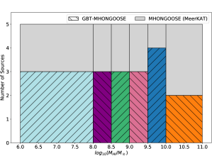
Figure 1: Histogram of Hi masses in the MHONGOOSE sample. Each bin is separated by color and hatch marking. The hatch markings (both directions) identify the GBT-MHONGOOSE sample and the gray solid represents the full MHONGOOSE with MeerKAT sample. This histogram demonstrates the coverage of the Hi mass range in the both MHONGOOSE samples. Note that the lowest and highest mass bins are larger due to the scarcity of galaxies meeting the survey criteria in those mass ranges.

3 Observations and Data Reduction

Observations for the 16 galaxies presented in S19 were carried out between August 2016 and January 2017 for project GBT16B-212. Each of these galaxies were observed for 10 hours each, a total of 160 hours, with a theoretical brightness temperature noise sensitivity of $\sim 13$ mK over $5.2\,\rm km\,s^{-1}$ channels. This noise sensitivity corresponds to a column density sensitivity of $N_{\rm HI}\,$$\sim 10^{18}\,\rm cm^{-2}$ over the same channel width. The two additional galaxies presented here (NGC 1744 and NGC 7424) were observed over the course of three GBT observing semesters (GBT15B-346, GBT16B-408, and GBT17A-478) from 2015 to 2017, for a total of 20 hours on NGC 1744 and 14 hours on NGC 7424. We observed these two galaxies over a bandwidth of 23.4 MHz, with a frequency resolution of 0.715 kHz. We used the sources 3C48 and 3C147, which have stable, well-understood fluxes, over the course of 12 observing nights to calibrate our data. We smoothed the data using a boxcar function with a final smoothed velocity resolution of $5.1\,\rm km\,s^{-1}$, or 24.3 kHz. The remainder of the data reduction followed the same approach presented in S19.

For each of our 18 galaxies, we used the GBT’s VErsatile GBT Astronomical Spectrometer (VEGAS) backend in L-band (1.15-1.73 GHz), where the FWHM beamwidth is $9.1^{\prime}$, to map $2^{\circ}\times\,2^{\circ}$ regions around each source. Data cubes were made for all 18 sources with pixel sizes of $1.75^{\prime}$. The 16 sources from S19 were smoothed to a velocity resolution of $6.4\,\rm km\,s^{-1}$.

We reached rms noise levels of 6 to 20 mK (3.2 - 10.4 mJy) in the cubes, corresponding to a $1\sigma$ column density sensitivity of $N_{\rm HI}\,$$=1.02\times 10^{17}\,\rm cm^{-2}$ per $5.1\,\rm km\,s^{-1}$ channel. At the noise level reached in this cube, a detectable signal at the $5\sigma$ level over a $20\,\rm km\,s^{-1}$ linewidth is $N_{\rm HI}\,$$=2\times 10^{18}\,\rm cm^{-2}$. Our $1\sigma$ mass sensitivities extend down to $1.6\times 10^{5}$ $\rm M_{\sun}$.

4 Properties of galaxies

Data cubes and integrated intensity (Moment 0) maps for the 16 sources mentioned above were inspected and searched for anomalous Hi in S19. In this section we will present the two additional sources, NGC 1744 and NGC 7424, and discuss their properties. These properties are listed in Table 2.

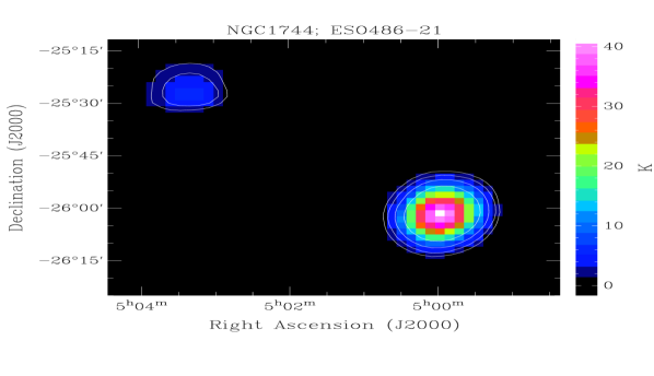
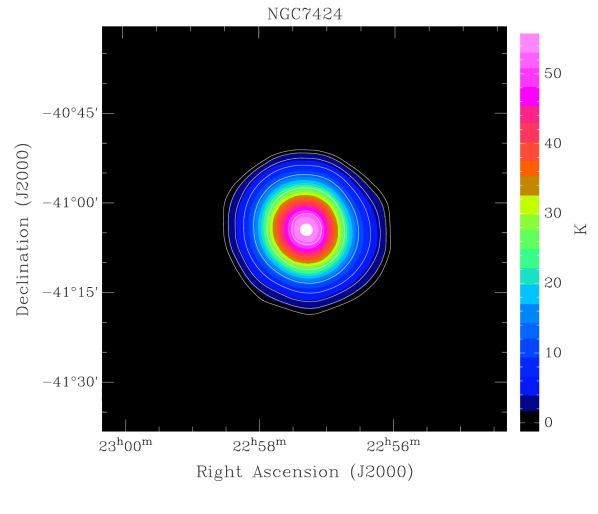
Figure 2: Left. Integrated intensity (moment 0) map of NGC 1744 with companion, ESO486-21 in upper left. Contours at 10, 20, and 40 times the integrated rms noise of 0.15 K. The column density equivalent to these contour levels is $N_{\rm HI}\,$= 0.69, 1.3, 2.7, and $5.5\times 10^{19}\,\rm cm^{-2}$. Right. Integrated intensity (moment 0) map of NGC 7424. Contours at 5, 10, 20, 40, 80, and 160 times the integrated rms noise of 0.16 K. The column density equivalent to these contour levels is $N_{\rm HI}\,$= 0.7, 1.48, 2.9, 5.9, and $11.9\times 10^{19}\,\rm cm^{-2}$.

4.1 NGC 1744

NGC 1744 is an inclined ($69.9^{\circ}$) SBcd galaxy. It is one of the more massive galaxies in our sample, which we measured the total Hi mass to be $7.6\times 10^{9}$ $\rm M_{\sun}$ ($\pm 2.1\times 10^{8}$). We measured a total integrated flux of 174.7 Jy km/s with an rms noise of $\sigma_{rms}=3.2$ mJy. We measured the full width at 20% maximum of the velocity profile to be 207.2 km/s with a systemic velocity of 743 km/s, which we used to calculate a dynamical mass (see subsection 5.2, equation 4) of NGC 1744 of $3.6\times 10^{10}$ $\rm M_{\sun}$. These and other properties of NGC 1744 were tabulated in Table 2 and discussed further in Section 5.

We detected one additional source in the NGC 1744 data cube. Sbc1 galaxy, ESO 486-G021 (Figure 3), is detected with an integrated Hi flux density of 24.5 Jy $\rm km\,s^{-1}$. The systemic velocities measured from the two galaxies differ by $\sim 100\,\rm km\,s^{-1}$, and while this is low enough to investigate potential interaction, we find their physical separation to be too great to make this likely. The angular separation is $58^{\prime}$, and at a distance of 12 Mpc, that becomes a physical separation of $\sim 200$ kpc. We calculated the Jacobi radius, the maximum radius expected of a central galaxy and companion galaxy system, with

$$r_{\rm J}=R_{Sep}\left(\frac{M_{Comp}}{3M_{Central}}\right)^{1/3}\,.$$ (1)

Here, $R_{Sep}$ is the physical separation between the centers of the two galaxies, $M_{Comp}$ is the dynamical mass of the companion galaxy, and $M_{Central}$ is the dynamical mass of the central galaxy. This gives us a maximum expected radius of $\sim 79$ kpc using the dynamical mass, derived from the Hi rotation velocity, of the companion of $2.2\times 10^{9}$ $\rm M_{\sun}$. It is evident that the 200 kpc projected separation is too large to consider plausible interaction. Further, we do not detect any extraplanar or anomalous Hi around NGC 1744 at these levels. A total Hi intensity map including both NGC 1744 and ESO 486-G021 can be seen in Figure 2. Spectra of NGC 1744 can be seen in Figure 3. At a mass sensitivity in this cube of $7.2\times 10^{5}$ $\rm M_{\sun}$, and because we did not detect any anomalous Hi , we can say that apart from ESO 486-G021 there are no additional sources with $3\sigma$ Hi mass greater than $7.2\times 10^{5}$ $\rm M_{\sun}$.

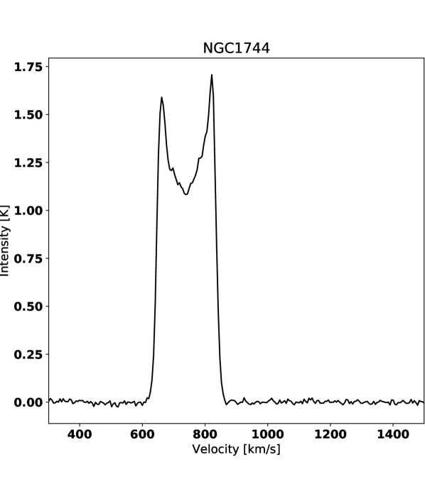
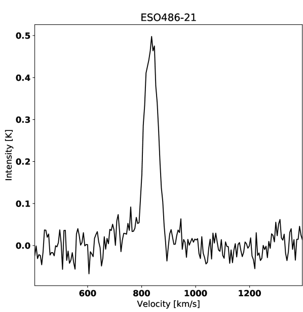
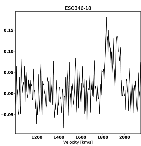
Figure 3: Total integrated Hi  profiles. Top row: NGC 1744 (left) and NGC 7424 (right). Bottom row: ESO486-21 detected in the NGC 1744 cube (left), and detected in the NGC 7424 cube is NGC7462 (center) and ESO346-18 (right).

4.2 NGC 7424

NGC 7424 is a mostly face-on SABcd galaxy (de Vaucouleurs et al., 1991), and one of the most Hi massive sources in the survey. It falls into the mass bin: $10<\rm log_{10}(M_{HI})<11$ $\rm M_{\sun}$, one of the more unexplored mass regimes in low column density Hi studies. We measured a total Hi mass of $2.4\times 10^{10}$ $\rm M_{\sun}$ ($\pm 6.2\times 10^{8}$) in NGC 7424, where the mass sensitivity in the cube is $2.3\times 10^{6}$ $\rm M_{\sun}$ corresponding to a $1\sigma$ column density sensitivity of $N_{\rm HI}\,$$=9.7\times 10^{16}\,\rm cm^{-2}$ per $5.1\,\rm km\,s^{-1}$channel. NGC 7424’s global Hi profile and moment map can be seen in Figure 3.

We detected two additional galaxies within our map of NGC 7424: the Sd galaxy ESO 346-G018 with an angular separation of $58^{\prime}$, and the SBbc galaxy NGC 7462 with an angular separation from NGC 7424 of $64^{\prime}$. However, due to their positions at the edges of our cube, we can not confidently measure the total Hi . Instead, we can provide the following lower limits. We measured an integrated flux of 8.8 Jy km/s for ESO 346-G018, with a linewidth at 20% maximum of 176 km/s around a systemic velocity of 1875 km/s. NGC 7462 has an integrated flux lower limit of 25.0 Jy km/s, a 20% maximum linewidth of 205 km/s, and a systemic velocity of 1066 km/s. The total integrated profiles were created for each galaxy and can be seen in Figure 3. No other significant detections of Hi were seen throughout the cube.

5 Analysis

Each source in this survey was analyzed by extracting information from the data cubes and deriving individual galaxy properties, followed by creating both masked and unmasked total integrated intensity (moment 0) maps, and measuring the global properties of the galaxy environments from these images. Moment 0 maps for each source can be found in S19. In doing this, we can identify the statistical properties over a wide population of galaxies.

5.1 Total integrated Hi  flux profiles

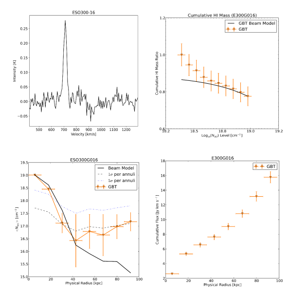
Figure 7: Same as Figure 4 for ESO 300-16.

We created total integrated Hi flux profiles for each galaxy using the MIRIAD task mbspect. mbspect makes a measurement of the data cube over a wide velocity range, where channels including emission are masked, and a first-order polynomial is fitted to the baseline, removing residual baseline variation. We obtain the $1\sigma$ rms noise over emission-free channel ranges, as well as the total integrated flux, and the linewidths of each source at 20% (W20) and 50% (W50) of the peak flux value. These measured values are listed in Table 2. Each galaxy’s global line profile can be seen in Figures 7 through 23.

5.2 Derived galaxy properties

For each data cube, we calculate the per channel $1\sigma$ column density sensitivity. We use measurements from mbspect to derive physical properties of each galaxy in the sample, such as the total Hi masses, total dynamical masses, and neutral gas fractions.

Column densities are calculated with

$$N_{\rm HI}=1.822\times 10^{18}\,\left(\frac{T_{\rm B}}{\rm K}\right)\,\left(\frac{dv}{\rm km\,s^{-1}}\right)\rm cm^{-2},$$ (2)

where $T_{\rm B}$ is the brightness temperature in units of Kelvin, and $dv$ is the resolution of our data in $\rm km\,s^{-1}$. When estimating the detectable column density level in the cube, we use a $5\sigma$ limit and a minimum linewidth of a typical Hi detection ($20\,\rm km\,s^{-1}$).

We integrate over the total flux values to estimate the Hi mass of each source, assuming the Hi is optically thin, using:

$$M_{\mbox{\sc{Hi}$\,$}}=2.36\times 10^{5}\,D^{2}\int_{v_{1}}^{v_{2}}S(v)dv\,\rm M_{\sun}.$$ (3)

Here, the distance, $D$, is in Mpc, and $\int_{v_{1}}^{v_{2}}S(v)dv$ is the total integrated flux over velocities enclosing the Hi profile $v_{1}$ to $v_{2}$, and is in units of Jy km $\rm s^{-1}$. The brightness temperatures from each cube were divided by the $1.86\,\rm K\,Jy^{-1}$ gain of the GBT to obtain units of Jy. We calculated this gain using an aperture efficiency of $\sim 0.65$ (Boothroyd et al., 2011) for the GBT at 1420 MHz.

In order to calculate the total dynamical mass of each galaxy, we first calculated the physical Hi diameter, $D_{\mbox{\sc{Hi}$\,$}}$, using the Broeils & Rhee (1997) scaling relation (Eq. 2.5), which is dependent on the optical diameter of the galaxy, $D_{25}$, measured at the $\rm 25^{th}\,mag\,arcsec^{-2}$ isophote in the B-band. We used values for $D_{25}$ from the Lyon-Meudon Extragalactic Database (LEDA). We use the dynamical mass equation:

$$M_{\rm dyn}=2.3\times 10^{5}\,\left(\frac{v_{rot}/sin(i)}{\rm km\,s^{-1}}\right)^{2}\left(\frac{r}{\rm kpc}\right)\rm M_{\sun},$$ (4)

where $v_{\rm rot}$ is the rotation velocity in $\rm km\,s^{-1}$, and $i$ the inclination, also taken from LEDA. These properties obtained from NED and LEDA can be seen in Table 1. We use our linewidth at 20% maximum to estimate $v_{\rm rot}$ as $v_{\rm rot}=W_{20}/2$. Dynamical masses are calculated inside the Hi radius, $r$ in kpc, calculated as $D_{\mbox{\sc{Hi}$\,$}}/2$.

The last property we derive using the information at hand, is the neutral Hi fraction. This is defined as the fraction of Hi mass in the galaxy and is calculated with $f_{\mbox{\sc{Hi}$\,$}}=M_{\rm HI}\,/\,M_{\rm dyn}$. Each of these derived properties are listed in Table 2 for every galaxy in the sample.

Table 1: Sample of MHONGOOSE Galaxies

Source	R.A.(J2000)	Decl.(J2000)	D	incl.	$D_{25}$	$\rm log_{10}M_{\star}$
	[h:m:s]	[∘:′:′′]	[Mpc]	[deg]	′	[$\rm M_{\sun}$]
ESO300G014	03:09:37	-41:01:50	12.9	61.2	4.47	8.72
ESO300G016	03:10:10	-40:00:11	9.3	35.6	0.78	…
ESO302G014	03:51:40	-38:27:08	11.7	27.6	1.35	7.79
ESO357-G007	03:10:24	-33:09:22	17.8	72.0	1.29	8.31
KK98-195	13:21:08	-31:31:45	5.2	55.7	0.45	…
KKS2000-23	11:06:12	-14:24:26	12.7	90.0	0.6	…
NGC1371	03:35:01	-24:56:00	20.4	47.5	4.9	10.7
NGC1592	04:29:40	-27:24:31	13.0	64.4	1.02	8.13
NGC1744	04:59:57	-26:01:20	10.0	69.9	5.25	9.19
NGC3511	11:03:23	-23:05:12	14.2	72.6	6.03	9.63
NGC5068	13:18:54	-21:02:21	6.9	30.1	7.41	9.32
NGC5170	13:29:48	-17:57:59	28.0	90.0	7.94	10.72
NGC5253	13:39:55	-31:38:24	3.0	70.1	5.01	8.57
NGC7424	22:57:18	-41:04:14	13.5	32.4	5.01	9.31
UGCA015	00:49:49	-21:00:54	3.3	67.4	1.62	6.74
UGCA250	11:53:24	-28:33:11	24.4	90.0	3.63	9.74
UGCA307	12:53:57	-12:06:21	8.6	62.0	1.82	7.96
UGCA320	13:03:16	-17:25:23	7.7	90.0	6.76	8.11

Note. — Positions listed in Columns 2-3 and distances in 4 gathered from NED. Inclination angles from face-on in columns 5 and the optical diameter, $D_{25}$, measured at the $\rm 25^{th}\,mag\,arcsec^{-2}$ isophote in the B-band values taken from HyperLEDA: http://leda.univ-lyon1.fr. Stellar masses were obtained from Leroy et al. (2019).

5.3 GBT beam model

One of the main science goals of this survey is to detect low column density Hi around our sample of galaxies. In order to distinguish between low column density Hi from an extragalactic source and the low level radiation entering the sidelobes of the GBT’s main beam, we use a beam model which measures these sidelobe levels precisely, modeling the beam response of an unresolved point source. We adopt the beam model used by Pingel et al. (2018). Without this model, emission entering the nearest sidelobes from the main beam could be confused for low column density emission from our sources. For each source in our sample, we used the GBT beam model as a template to regrid each data cube to have $4^{\prime\prime}$ pixels with size $1024\times 1024$ using the MIRIAD tasks imgen and regrid.

5.4 Integrated intensity images (Moment 0)

We created integrated intensity images, or Moment 0 images, for each source in our sample. An unmasked image was made by integrating pixel values over a channel range in the data cube containing emission from the central source. We also created masked Moment 0 images with the intention of separating signal from noise when searching for low column density Hi . In order to do this, we set to zero the pixels with values below three times the noise in that cube, and again integrate over the same channel range. After integration over the channel range we selected, we expect the $\sigma_{rms}$ noise in each map (masked and unmasked) to increase by a factor of:

$$\sigma_{N}=\sqrt{N}\,\sigma_{rms}$$ (5)

where $N$ is the number of channels integrated over, and $\sigma_{rms}$ is the root-mean-squared noise per channel in the data cube. We calculated a $1\sigma$ noise map for both the masked and unmasked images this way. We then create our maps using a $3\sigma$ cutoff in the same way as Pingel et al. (2018) by creating a signal-to-noise (S/N) map for both the masked and unmasked images. The S/N map for the unmasked image is made by dividing the unmasked integrated image by the unmasked $1\sigma$ noise map, while the masked S/N map is created by dividing the image where pixels below $3\sigma_{rms}$ were set to zero by the masked $1\sigma$ noise image. From each of these S/N maps, we calculated a $3\sigma$ threshold by taking the mean value of the pixels with S/N values falling between 2.75 and 3.25. We then use this new $3\sigma$ value to mask, or set to zero, the pixels in our masked integrated image that fall below this value. In doing this, we are confident in our characterization of the noise in our maps.

5.5 Cumulative Hi  vs. $N_{\rm HI}\,$

We want to find out how much Hi mass is contained at different column density levels in each galaxy. In doing this, we will be able to identify the amount of low column density Hi in the galaxy as a percentage of the total Hi mass. Accordingly, in the way described in Pingel et al. (2018), we bin the column densities above the $3\sigma$ level in our unmasked image and calculate the percentage of Hi mass that falls into each $N_{\rm HI}\,$bin by converting each pixel in the image to a column density level, and subsequently into an Hi mass. We determine the percentage of Hi mass at or above a given column density bin, and can therefore quantify the percentage of Hi mass below some column density threshold. Each galaxy is normalized to that galaxy’s maximum Hi mass in the cumulative Hi vs. $N_{\rm HI}\,$plots in Figures 7 through 23.

In addition to the data from each cube, we use the beam models described above to determine whether each source can be reliably analyzed. Each beam model for each galaxy is scaled to the maximum column density of the associated GBT image from the data and we analyze it in the same way as the GBT images described in the previous paragraph, calculating the cumulative Hi mass in each $N_{\rm HI}\,$bin. In doing this, we can determine if the source is following the response of the GBT beam or deviating from it. If the source follows the beam, we can determine that the source is unresolved, and therefore does not satisfactorily fill the beam, causing the Hi column density to spread out over the beam area appearing as if low column density Hi was detected. To this end, we would omit these unresolved sources from our statistical analysis of the disk. We distinguish which sources are unresolved by looking at the cumulative Hi mass ratio of the data versus the model. If the data follows the beam response of the model, we determine that source to be unresolved. Data points above the model is characterized as resolved, and if the error bars fully clear the beam model, we categorize it as very well resolved.

We can infer additional information about the amount of low column density Hi in the galaxy by looking at the shape of the profile in relation to the GBT beam model. If a source contains excess diffuse Hi , we will see a positive deviation in the data at low column densities as compared to the beam model. Several of the resolved sources follow the shape of the beam model, and they flatten out at or above the $3\sigma$ column density threshold described in Section 5.3, which is indicative of the scarcity of low column density Hi in that galaxy. If, instead, we see an increase at low column densities as compared to the beam model, then we know we are detecting an excess of low column density Hi within that halo, which could be diffuse gas or clumpy material spread over the beam. This excess could be the result of a number of scenarios including detection of a low column density companion, extended or clumpy Hi clouds, the presence of a $>3\sigma$ noise artefact, or the detection of accretion of low column density Hi from the CGM. For each image showing a higher fraction of low column density Hi , we search for $>3\sigma$ artefacts in order to rule out that possibility, and look for higher S/N regions in both the cubes and the integrated images.

Table 2: Hi Measurements and Derived Properties of MHONGOOSE Galaxies

Source	$\sigma_{rms}$	$S_{\mbox{\sc{Hi}$\,$}}$	$\rm V_{sys}$	$\rm W_{50}$	$\rm W_{20}$	$\rm log_{10}$$N_{\rm HI}\,$1σ	$\rm log_{10}$$N_{\rm HI}\,$3σ	$\rm log_{10}M_{1\sigma}$	$\rm log_{10}M_{\mbox{\sc{Hi}$\,$}}$	$\rm log_{10}M_{dyn}$	$f_{\mbox{\sc{Hi}$\,$}}$
	[mJy]	[$\rm Jy\,km\,s^{-1}$]	[$\rm km\,s^{-1}$]	[$\rm km\,s^{-1}$]	[$\rm km\,s^{-1}$]	[$\rm cm^{-2}$]	[$\rm cm^{-2}$]	[$\rm M_{\sun}$]	[$\rm M_{\sun}$]	[$\rm M_{\sun}$]
ESO300G014	10.4	33.6	955.0	129.2	145.2	17.35	18.33	6.42	9.12	10.36	0.058
ESO300G016	9.1	4.9	710.5	30.1	43.9	17.29	18.27	6.07	8.0	8.78	0.167
ESO302G014	9.6	13.7	869.3	65.5	87.1	17.31	18.29	6.29	8.65	9.91	0.055
ESO357-G007	4.9	15.0	1118.3	118.4	148.5	17.02	18.0	6.37	9.05	9.91	0.137
KK98-195	5.9	8.1	570.6	27.1	42.2	17.1	18.08	5.38	7.71	7.95	0.577
KKS2000-23	5.3	14.2	1037.5	80.2	96.8	17.06	18.03	6.11	8.73	9.02	0.515
NGC1371	7.6	90.9	1454.3	386.4	403.8	17.21	18.19	6.68	9.95	11.63	0.021
NGC1592	4.8	5.8	942.9	55.1	96.2	17.01	17.99	6.08	8.36	9.34	0.104
NGC1744	3.2	174.7	743.4	191.1	207.2	16.75	17.82	5.59	9.62	10.56	0.112
NGC3511	8.3	74.6	1130.8	272.4	308.7	17.25	18.23	6.4	9.55	11.11	0.028
NGC5068	4.8	191.5	667.7	67.9	108.0	17.01	17.99	5.53	9.33	10.53	0.063
NGC5170	6.2	106.2	1546.7	504.0	523.0	17.13	18.1	6.87	10.29	11.94	0.023
NGC5253	8.3	57.6	404.5	63.4	99.1	17.25	18.23	5.05	8.09	9.38	0.051
NGC7424	5.6	297.2	934.9	152.6	170.5	16.99	18.06	6.1	10.11	10.99	0.13
UGCA015	5.2	5.2	293.6	25.5	43.2	17.05	18.02	4.93	7.12	8.23	0.078
UGCA250	7.6	87.6	1700.6	272.2	289.5	17.21	18.19	6.83	10.09	11.03	0.115
UGCA307	5.0	32.0	822.9	68.5	95.2	17.03	18.01	5.74	8.75	9.42	0.211
UGCA320	7.8	133.9	749.1	106.3	126.9	17.23	18.2	5.84	9.27	10.08	0.156

Note. — (1) Source name. (2) measured rms noise. (3) Total integrated flux. (4) Systemic velocity. (5) Linewidth at 50% maximum. (6) Linewidth at 20% maximum. (7) $1\sigma_{rms}$ column density sensitivity per channel. (8) $3\sigma_{rms}$ column density level over a 20 $\rm km\,s^{-1}$ linewidth. (9) Hi mass sensitivity. (10) Hi mass. (11) Dynamical mass. (12) Neutral gas fraction.

5.6 Radial $N_{\rm HI}\,$

We also want to determine how Hi  column densities ($N_{\rm HI}\,$) behave as a function of distance from the galaxy. The optimal way of identifying abundances in low column density Hi is to take the average of the Hi column density levels in annuli around the galaxy. This allows us to characterize the azimuthally averaged $N_{\rm HI}\,$at various physical galaxy radii. We define the annuli for each galaxy using the masked rather than unmasked images so as to reduce the effect of quantifying low level noise as signal. Each image is regridded to have $1024\times 1024$ pixels corresponding to $4^{\prime\prime}$ per pixel for the purpose of precision when quantities inside each annulus are calculated. The GBT beam’s FWHM of $9.1^{\prime}$ sets a lower limit to the radius of the smallest annulus to be $4.5^{\prime}$, or $\sim 68$ pixels. The maximum radius of the largest annulus is calculated as the largest multiple of the 68 pixel radius that lies within the image size. For most of our sources, we calculate this to be eight annuli, and for images in which we use a smaller region around the galaxy, we end up with five annuli. The $N_{\rm HI}\,$within each annulus is then averaged by summing the values greater than $3\sigma$ and dividing this by the total number of pixels in the annulus. Dividing by the total, rather than the number of pixels above $3\sigma$, we run the risk of underestimating the average $N_{\rm HI}\,$in the annulus, but we are avoiding a bias toward higher $N_{\rm HI}\,$values which would result from the average using only values $>3\sigma$.

Once again, we want to be able to compare the data against the GBT beam model to look for deviation from the response of the beam. Each model is scaled to the maximum $N_{\rm HI}\,$value in the image, and drops off at larger radii. The galaxies in our sample follow the response of the beam at low radii, and begin to flatten out around the $3\sigma$ threshold. Some of the galaxies flatten out above this threshold, which could indicate a smooth extent of the galaxy rather than an ionization edge at a particular column density level around that galaxy. The $1\sigma$ and $5\sigma$ thresholds are indicated for each galaxy as the dashed horizontal lines in Figures 7 through 23.

We can also infer details about the environments of these galaxies by looking at the shape of the radial $N_{\rm HI}\,$profile. If the data follows the noise levels out to large radii, we can then say that there is no low column density Hi surrounding that galaxy for levels at or above the rms noise sensitivity reached in that cube. However, several of the galaxies show a positive deviation in the averaged $N_{\rm HI}\,$at these large radii. For each galaxy in which this positive deviation is identified, we investigate the cube and integrated maps in order to identify a source for the excess Hi . The excess could be due to detection of a companion, an extended Hi cloud, a higher $\sigma$ noise spike, or the accretion of Hi onto the galaxy from the CGM.

5.7 Radial Flux

We can trace the flux in each galaxy out to the same physical radii that we explored in the radial $N_{\rm HI}\,$analysis using the same method to calculate each annuli. We use the unmasked images for this analysis as this is the best way to characterize the total flux of the galaxy at various radii, since our unmasked images contain all the flux detected from the source.

Since we are measuring the cumulative flux at physical radii, we should see the profile continue to increase linearly as the area inside each annulus increases linearly if the average $N_{\rm HI}\,$described above is flat. If the radial flux profile deviates from a positive linear trend, we know to look for an increase in low column density gas around that galaxy. A dip in the profile is likely indicative of an unphysical negative feature in the image, causing the cumulative flux to decrease at that radius. If indeed we see rising cumulative flux levels at increasing radii, these would be consistent with the detection of Hi at large impact parameters as is seen in Das et al. (2020) where Hi is detected at each point along the minor axis out to $\sim 120$ kpc.

6 Results

Most of the galaxies in our sample are moderately to well-resolved in the GBT beam, and give us reliable statistical properties. As described in Section 5.5, a resolved source is defined by a positive offset of the data from the GBT beam model in the cumulative Hi mass vs. $N_{\rm HI}\,$plots and in the radially averaged $N_{\rm HI}\,$vs. physical radius plots. The plots in Figures 7 through 23 show, clockwise from top left, the total integrated Hi profile vs. velocity, the cumulative Hi mass vs. $N_{\rm HI}\,$, the cumulative flux vs. physical radius, and the azimuthally averaged $N_{\rm HI}\,$levels vs. physical radius. For reference, we have put this analysis for NGC 7424 in Figure 4, while the remainder of the analysis for each galaxy in our sample can be found in the Appendix. The results from analysis of all of our sources will be described below, and they have been grouped by low (Bin 1), intermediate (Bins 2-5), and high (Bin 6) Hi mass displayed in Figure 1.

6.1 Low $M_{\rm HI}\,$($6<\rm log_{10}(M_{HI})<8$ $\rm M_{\sun}$)

Figure 7 displays a very slight positive offset of ESO 300-16 from the GBT model in the cumulative Hi mass vs. column density, where the lowest column density levels deviate in the positive direction. At the smallest radii seen in the radially averaged $N_{\rm HI}\,$plot, we can see that this source is not well resolved until we move beyond the disk, where our underestimated $N_{\rm HI}\,$values are consistent with the noise and begin to rise. The cumulative flux continues to rise even at large distances from the disk.

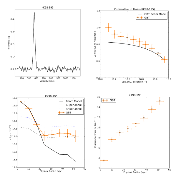
Figure 8: Same as Figure 4 for KK98-195.

We see the response of the data in the plots of KK98-195 (Figure 8) are fairly unremarkable. We see a very slight positive deviation of the cumulative Hi mass as compared to the GBT beam model at the lowest $N_{\rm HI}\,$level, demonstrating a small fraction (less than 10%) of the Hi mass in the galaxy to be at the lowest column densities. The average $N_{\rm HI}\,$flattens outside the disk in the radially averaged $N_{\rm HI}\,$plot, and the flux increases linearly in the cumulative flux plot.

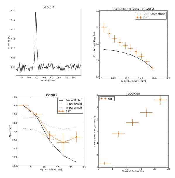
Figure 9: Same as Figure 4 for UGCA015.

UGCA015 (Figure 9) is $\sim 40^{\prime}$ in angular distance from the large galaxy, NGC 247, which shows up in our data cube at overlapping velocities. For this reason, we analyzed a smaller region around UGCA015 in order to exclude possible emission from NGC 247. We see a positive offset in the Hi mass at the lower column densities. While we were not able to extend out to farther radii, we note that the cumulative flux again does not begin to flatten beyond the disk.

Peak column densities in each of these low $M_{\rm HI}\,$galaxies sit right around $N_{\rm HI}\,$$=10^{19}\,\rm cm^{-2}$. None of the three galaxies in this mass range display any positive deviation from the noise level in the azimuthally averaged $N_{\rm HI}\,$plots, but each one shows an increase in the fraction of Hi mass at the lowest column densities. The largest of these fractions comes from UGCA015, where the offset from the beam model deviates significantly, making up over 20% of the mass fraction from the lowest column densities. Each of the radially averaged cumulative flux profiles continue to rise as far as our maps reach. This indicates that we have not yet reached the end of the Hi emission in our maps of these smallest galaxies.

Figure 4: Top left: Total integrated Hi profile. Top right: Cumulative Hi mass. The total Hi mass in the moment 0 map is plotted by the fraction of gas in column density bins, and compared to the GBT beam model, scaled to the peak column density. Lower left: Azimuthally averaged $N_{\rm HI}\,$. Column density averaged over annuli extending radially from the center of the galaxy and compared to the GBT beam model. The black dashed line characterizes the $1\sigma$ noise in each annulus, and the blue dot-dash line represents the $5\sigma$ noise in each annulus. Lower right: Cumulative flux. Flux in each of those annuli are summed to obtain a measure of the total flux out to the edge of each map.

6.2 Intermediate $M_{\rm HI}\,$($8<\rm log_{10}(M_{HI})<10$ $\rm M_{\sun}$)

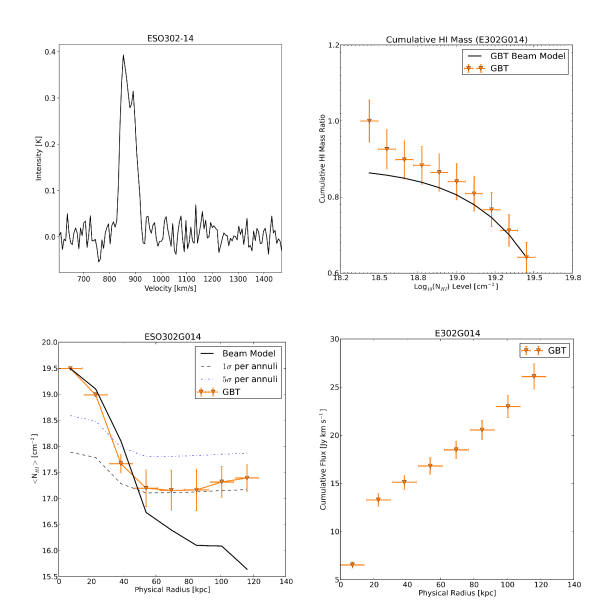
Figure 10: Same as Figure 4 for ESO 302-14.

Figure 10 displays the properties of ESO 302-14, where we see an increase at the lowest column densities in the cumulative Hi mass plot, flattening outside the disk in the radially averaged $N_{\rm HI}\,$plot, and increasing flux levels in the cumulative flux plot. de Blok et al. (2020) detect a filament extending off the disk of ESO 302-14 as well as an Hi cloud with a peak column density of $N_{\rm HI}\,$$=4\times 10^{19}\,\rm cm^{-2}$ about 30 kpc south of the center of the galaxy. These structures are significantly smaller than the FWHM beamwidth of the GBT and this emission would be spread out over the beam, diluting the signal.

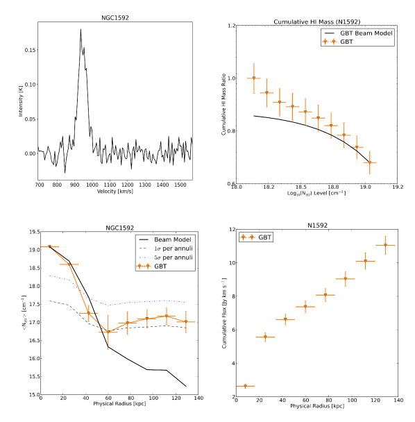
Figure 11: Same as Figure 4 for NGC 1592.

NGC 1592 (Figure 11) has a peak column density level of just over $N_{\rm HI}\,$$=10^{19}\,\rm cm^{-2}$. The cumulative flux rises at large radii.

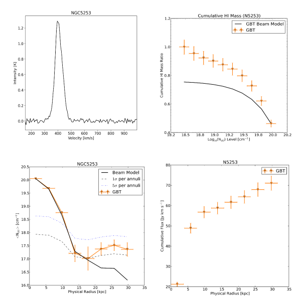
Figure 12: Same as Figure 4 for NGC 5253.

The properties of NGC 5253 are shown in Figure 12. There is an increase in the azimuthally averaged column density levels around 25 kpc, which is associated with one bright region in the integrated intensity (moment 0) image. This bright region has no associated optical counterpart, previously identified Hi cloud, nor does the spectra show anything we would consider to be RFI. Thus, we considered it to be a candidate for accretion of Hi onto the galaxy.

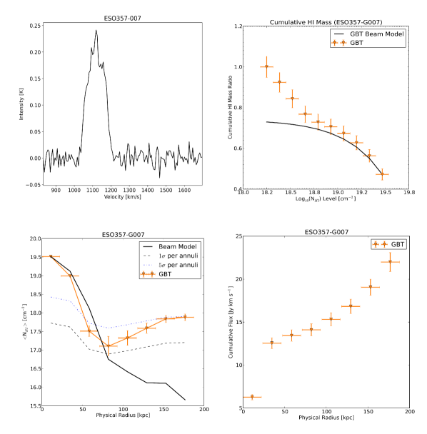
Figure 13: Same as Figure 4 for ESO 357-007.

ESO 357-007 (Figure 13) contains increasing amounts of diffuse Hi beginning around $N_{\rm HI}\,$$=10^{18.8}\,\rm cm^{-2}$, comprising over 20% of the cumulative Hi mass fraction. We can see in the azimuthally averaged $N_{\rm HI}\,$plot that the galaxy does not appear to be resolved in the GBT beam at low physical radii of the galaxy, and displays an increasing average $N_{\rm HI}\,$at the radii beyond the disk. The cumulative flux does show a non-linear increase at the largest physical radii mapped. In the absence of evidence of a companion galaxy, or any bright artefact in the data cube causing the cumulative flux to increase, we are led to believe that this evidence of excess neutral hydrogen at large radii could be accretion through the CGM onto ESO 357-007. Alternatively, this excess of low column density Hi could be indicative of a large reservoir of Hi sitting in the halo of ESO 357-007.

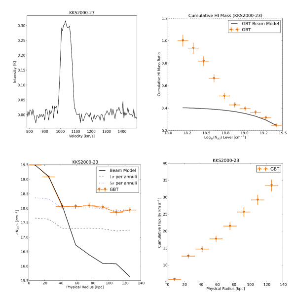
Figure 14: Same as Figure 4 for KKS2000-23.

KKS2000-23 shows a significant portion of its Hi mass to be made up of low column density gas, as can be seen in the cumulative Hi mass plot in Figure 14. However, inspection of the data cube and the moment map reveal a higher level of noise in the image, making it difficult to determine if the low column density gas comes from real emission or is some artefact from the observation. This particular issue could be alleviated with additional observations to verify the presence or absence of low $N_{\rm HI}\,$gas.

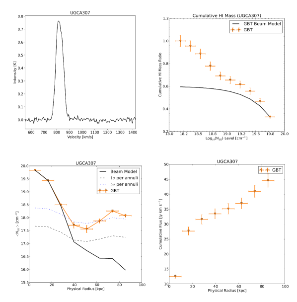
Figure 15: Same as Figure 4 for UGCA307.

UGCA307 also shows an increase in low column density gas in Figure 15. However, the azimuthally averaged $N_{\rm HI}\,$vs. physical radius displays a steep increase between 55 kpc and 65 kpc. We inspected the data cube and discovered a small galaxy, which we believe is LCRS B125208.8-112329, residing 72 kpc away in projected distance. This can also be seen in the cumulative flux vs. physical radius plot, where the flux increases around the same physical distance. This would be the first velocity information available for this galaxy, with a central velocity of 863 km/s.

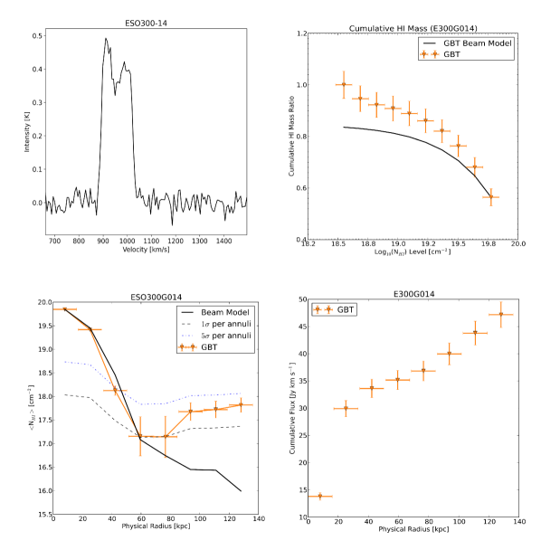
Figure 16: Same as Figure 4 for ESO300-14.

The spiral galaxy ESO 300-14 can be seen in Figure 16. The total integrated flux of ESO 300-14 displays the expected double horn feature for an inclined, rotating galaxy. It is resolved in the GBT beam, where the cumulative flux follows the shape of the GBT beam model, and is positively offset in relation to that model. The azimuthally averaged column densities vs. physical radius show a rising $N_{\rm HI}\,$level outside the disk, and the cumulative flux at increasing physical radii increases linearly.

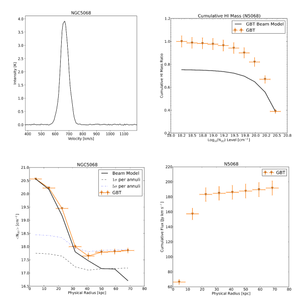
Figure 17: Same as Figure 4 for NGC 5068.

Similarly, the face-on galaxy, NGC 5068, exhibits similar behavior when comparing these same properties. The cumulative Hi mass plot in Figure 17 shows that $\sim 99\%$ of the mass in the galaxy is seen in column densities above $N_{\rm HI}\,$$=10^{19}\rm\,cm^{-2}$. This is substantiated in both the average $N_{\rm HI}\,$and cumulative flux vs. physical radii plots, where there is no evidence of an increase in Hi gas at large radii.

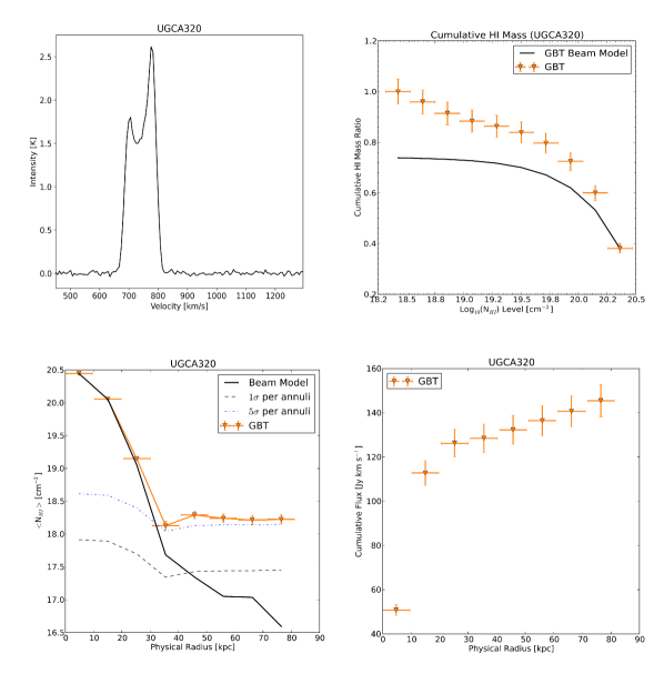
Figure 18: Same as Figure 4 UGCA320.

We detected two additional sources in the region close to UGCA320: UGCA319 at $\sim 41$ kpc, and a second detection around $\sim 61$ kpc projected distances. The closer companion, UGCA319 can be seen as a slight bump in the averaged $N_{\rm HI}\,$around $\sim 45$ kpc in Figure 18. The second Hi detection lacks a known counterpart in Hi , but may be associated with the small galaxy LEDA 886203, the only optical galaxy near this position. These two companions are likely what is causing the gradual increase in cumulative Hi flux at radii larger than 40 kpc. This would also be the first redshift information available on LEDA 886203 with a central velocity of 727 km/s.

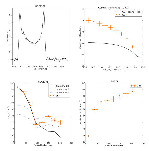
Figure 19: Same as Figure 4 for NGC 1371.

NGC 1371 is well-resolved in the GBT beam, as seen in the cumulative Hi mass plot in Figure 19. In most of these plots, NGC 1371 behaves as expected, with the exception of an artefact at $\sim 150$ kpc as seen in the radially averaged $N_{\rm HI}\,$plot.

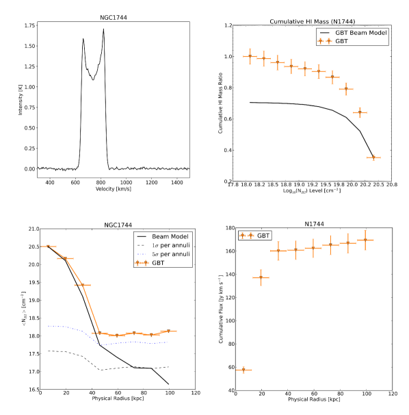
Figure 20: Same as Figure 4 for NGC 1744.

One of our more massive galaxies, NGC 1744, shows no signs of excess amounts of low column density gas as seen in the cumulative Hi mass plot in Figure 20. We can see in the radially averaged $N_{\rm HI}\,$plot that this source is well-resolved, and shows an unusually high average $N_{\rm HI}\,$at radii beyond the disk. This could be indicative of smooth accretion of Hi , a reservoir of Hi halo gas, or a higher noise floor than we had estimated.

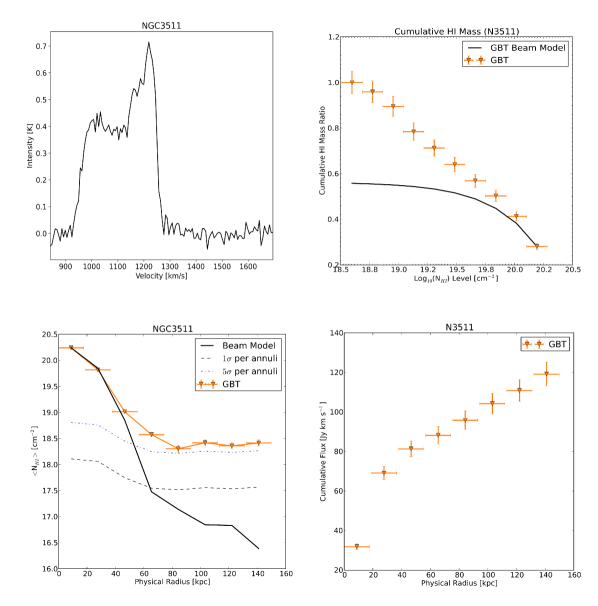
Figure 21: Same as Figure 4 for NGC 3511.

NGC 3511 (Figure 21) shows large deviation at low column density levels, where the cumulative amount of Hi increases almost linearly through $N_{\rm HI}\,$$=10^{18.6}\,\rm cm^{-2}$. It is resolved in the GBT beam as seen in both the cumulative mass plot and the averaged $N_{\rm HI}\,$plot. Similar to NGC 1744, this source displays higher $N_{\rm HI}\,$values out into the halo.

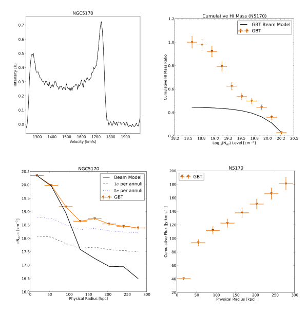
Figure 22: Same as Figure 4 for NGC 5170.

NGC 5170, in contrast with NGC 1744 which resides in the same mass bin, does show an increase towards lower column density Hi mass. Figure 22 reveals a sharp change in the slope of the cumulative Hi mass at column densities lower than $\sim 10^{19.4}\,\rm cm^{-2}$. The azimuthally averaged $N_{\rm HI}\,$plot does show an increase in average $N_{\rm HI}\,$around 175 kpc. Inspection of the moment 0 image reveals some bright, filamentary structure at the same physical distance, which could be accreting Hi gas. Without any indication of a nearby optical counterpart associated with those bright regions which appear to lack optical counterparts, we consider this a candidate for accretion from the CGM.

6.3 High $M_{\rm HI}\,$($10<\rm log_{10}(M_{HI})<11$ $\rm M_{\sun}$)

We can see NGC 7424, one of the most Hi massive galaxies in our sample, in Figure 4. The data in the averaged $N_{\rm HI}\,$vs. physical radius plot shows slightly higher and gradually increasing values of $N_{\rm HI}\,$at radii outside the disk. Visual inspection of the image did not reveal any regions of particular interest.

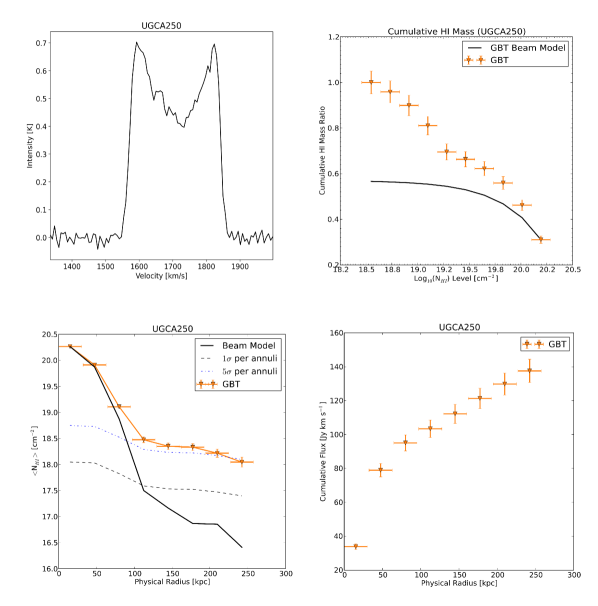
Figure 23: Same as Figure 4 for UGCA250.

One of our largest sources, UGCA250 (Figure 23), occupies our highest mass bin: $10<\rm log_{10}(M_{HI})<11$ $\rm M_{\sun}$. The cumulative Hi mass increases at low column densities, and the cumulative flux continues to grow linearly as the radius increases. Inspection of the data cube revealed a bright, positive stripe across the top of UGCA250, at the same declination as another bright source on the edge of our cube, UGCA247. Within that stripe is a possible new Hi detection which is coincident with the only catalogued galaxy within the size of the GBT beam at this position, FLASH J115508.00-282045.1 at a radius of $\sim 185$ kpc.

7 Discussion

7.1 Hi in the CGM

Our analysis of the cumulative Hi mass allowed us to quantify the total Hi mass in the moment maps. Our maps were made at a constant angular size of $2^{\circ}\times 2^{\circ}$, so we do not have a consistent physical region around each mapped source where initial map sizes range from 105 – 977 kpc on one side. The measurement of the Hi mass is made in the moment map where we can subtract off the Hi mass of the disk, which is derived from the integrated spectra of each galaxy. The total Hi mass in the moment map less the integrated Hi disk mass from the spectra gives us some value for the amount of mass outside the disk. We refer to this amount as $f_{CGM}$. This fraction represents the total amount of Hi mass in the CGM in relation to the Hi disk mass: $f_{CGM}=\rm M_{CGM}/M_{disk}$. Out of our 18 galaxies, 16 contained an excess amount of gas outside their disk by 0.02 to 3 times the amount of Hi in the disk. The only two galaxies we did not detect Hi in their CGM were NGC 1744 and NGC 7424. We can see this in both the cumulative Hi mass plots and the cumulative flux plots for both of these galaxies. In both of these galaxies, the cumulative Hi mass stays mostly flat at column densities below its turnover ($N_{\rm HI}\,$$\lesssim 10^{19.5}\,\rm cm^{-2}$) and the cumulative flux does not rise at large distance from the galaxy. This same flattening also occurs with NGC 5068, which contains only 2% more Hi outside its disk. This tells us that there is very little, if any, low column density gas outside the disks of these three galaxies. We generally find that maps covering a smaller physical area contain a smaller total amount of $M_{\rm HI}\,$outside of the disk, and larger physical maps contain a larger total amount of $M_{\rm HI}\,$outside of the disk. This may seem like an intuitive result if Hi  permeates the CGM of most galaxies, and yet it has evaded most observational studies of Hi emission in the CGM of galaxies. This result is consistent with Das et al. (2020) where Hi emission was detected in each measurement at increasing distances along the minor axis of the two galaxies, NGC 891 and NGC 4565. These detections could be the outcome of ubiquitous CGM Hi which, in mapping observations such as this current work, would result in a larger amount of Hi detected over larger physical areas. A study of this type could be improved on with a consistent physical parameter guiding the size of the area observed, such as the virial radius of a galaxy. Mapping the full extent of the halo, as the upcoming Parkes-IMAGINE survey (Sardone et al., in prep) will do, would give insight into the amount of Hi  permeating the entire CGM of a galaxy.

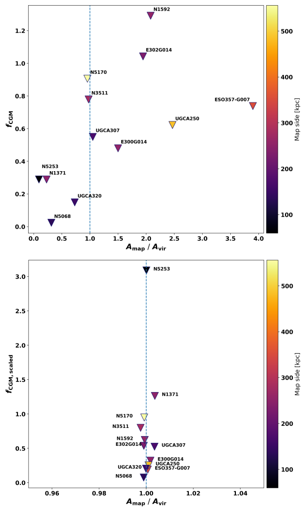
Figure 5: Top. The amount of Hi detected in the CGM as a fraction of the Hi disk mass. These CGM mass measurements were taken throughout the map area and are shown relative to the target galaxy’s virial area. The colorbar identifies the physical size of the map. The blue dashed line indicates a map area equal to the virial area. Bottom. The fraction of mass in the CGM in the top plot now scaled such that each map area is equal to its virial area. Triangles offset for visual ease.

As our physical map sizes are not uniform, we would like to know how the fraction of Hi mass in the CGM would change, assuming smooth coverage of the gas, if each galaxy were mapped precisely to its virial radius, calculated from the virial mass found using the Moster et al. (2010) stellar-to-halo-mass relation. We show this change in Figure 5 where our empirical measurements are shown in the top panel, and a scaled version is shown in the lower panel. We find that as an increasing fraction of the halo is probed, and in several cases multiple times the halo, the fraction of Hi gas in the CGM also increases. The largest value of $f_{CGM}$ comes from the map of NGC 1592. We made measurements over an area twice the size of its halo and found 1.3 times the amount of Hi disk mass in the surrounding area. However, when scaled the map to cover precisely one halo area, $A_{\rm map}/A_{\rm{vir}}=1$, this fraction reduces to 0.62 times the Hi disk mass. We note that the scaled fractions, $f_{\rm CGM,scaled}$, reveal an outlier containing three times the amount of Hi mass in its CGM, NGC 5253, which we earlier identified as a candidate for accretion. We discuss this further in the following sections.

7.2 Fraction of low $N_{\rm HI}\,$

We define a characteristic column density as low $N_{\rm HI}\,$if it is below a level of $10^{19}\,\rm cm^{-2}$. This value is taken from the prediction that below $\sim 10^{19}\,\rm cm^{-2}$ the amount of hydrogen in the neutral phase is truncated, and the gas transitions from mostly neutral to mostly ionized, making detections much below this level difficult, although not impossible. This sharp drop is largely due to photoionization of the neutral hydrogen by the extragalactic radiation field and represents one way of defining the edge of an Hi disk. This was first explained by Bochkarev & Siuniaev (1977) and later by Maloney (1993) who suggested that the ionization fraction sharply increases at a critical column density of a few times $10^{19}\,\rm cm^{-2}$, irrespective of galaxy mass or halo parameters. An example of this sharp drop-off in Hi is the KAT-7 observations of M83, which revealed a steep decrease in $N_{\rm HI}\,$at the edge of the galaxy disk (Heald et al., 2016). Recently, Bland-Hawthorn et al. (2017) demonstrated that it may be possible to detect low column density Hi at significantly larger radii than the predicted truncation radius from Maloney (1993). Specifically, they showed that the radius at which 50% of the total amount of hydrogen is ionized is significantly larger. These results seem to be congruent with those of Ianjamasimanana et al. (2018) who investigated radially averaged column density profiles of 17 galaxies in search of a break at the $\sim 10^{19}\,\rm cm^{-2}$ level and found no evidence for a sharp change anywhere above their detection limits.

We determined the diffuse neutral fraction for each galaxy using (Pingel et al., 2018):

$$f_{19}=1-\frac{M_{19}}{M_{\mbox{\sc{Hi}$\,$}}}\,.$$ (6)

In this equation, the diffuse neutral fraction, $f_{19}$, is defined by the fraction of Hi below column densities of $10^{19}\,\rm cm^{-2}$, where $M_{19}$ is the Hi mass at column density levels $N_{\rm HI}\,$$\geq 10^{19}\,\rm cm^{-2}$ and $M_{\mbox{\sc{Hi}$\,$}}$ is the total Hi mass as determined in Section 5.5. Values of $f_{19}$ are listed in Table 3.

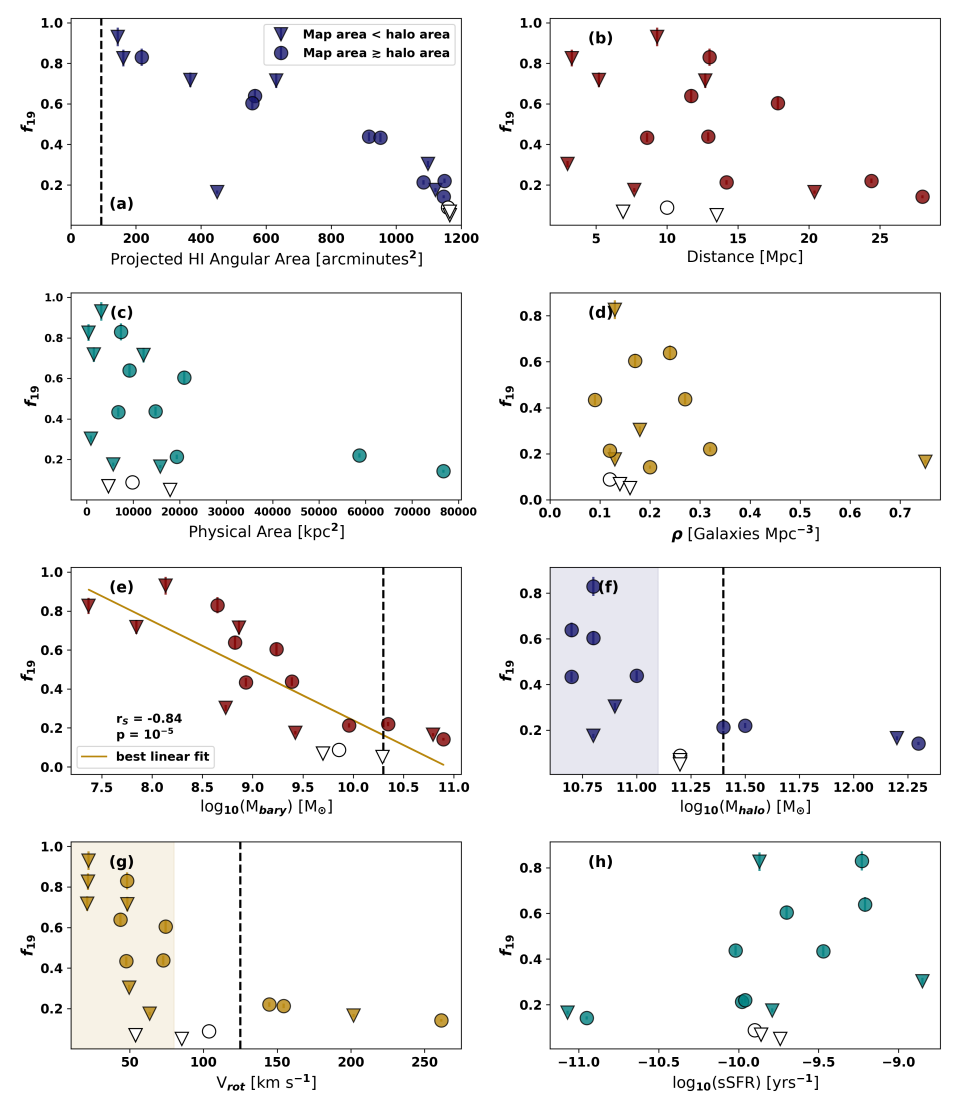
Figure 6: Comparisons of the diffuse neutral fraction for each GBT-MHONGOOSE galaxy. Circles represent measurements over an area larger than or equal to the area of the halo. Triangles represent measurements over a region smaller than the halo and should be interpreted as a lower limit. The three galaxies (NGC 5068, NGC 1744, NGC 7424) whose cumulative flux profiles flatten at large radii, indicating the Hi has truncated, are shown as unfilled markers. (a) Angular areas calculated inside region where column densities reach $N_{\rm HI}\,$$>1\times 10^{19}\,\rm cm^{-2}$. Vertical dashed line represents the angular area of the $9.1^{\prime}$ FWHM GBT beam. (b) Distance. (c) Physical areas calculated from the $N_{\rm HI}\,$$=1\times 10^{19}\,\rm cm^{-2}$ angular diameter. (d) Galaxy density. (e) Baryonic mass using $\rm M_{bary}=1.36\cdot M_{\mbox{\sc{Hi}$\,$}}+M_{*}$. Vertical dashed line at the cold accretion threshold given in Kereš et al. (2005). We show a best fit line through the data revealing, rather than a firm threshold for cold accretion, a correlation between a galaxy’s baryonic mass and its diffuse gas fraction. The strength of this correlation is demonstrated with the Spearman correlation coefficient and the associated p-value. (f) Dark matter halo mass derived from the Moster et al. (2010) relation. Vertical dashed line at threshold also given in Kereš et al. (2005). The shaded region marks a lower threshold showing, based on low $N_{\rm HI}\,$measurements from this work, the regime in which cold accretion is more likely. (g) Rotation velocity using $\rm V_{rot}=W_{20}/2$. A vertical dashed line at 125 km/s shows the threshold suggested by Kannappan et al. (2013), below which galaxies become dominated by their gas. We mark a shaded region, based on this work, demonstrating a lower threshold for a diffuse gas dominated regime below 80 km/s. (h) Specific star formation rate calculated using SFR from Leroy et al. (2019).

With our $f_{19}$ values in hand, we would like to compare the diffuse neutral fraction as a function of galaxy parameter, such as galaxy density, baryonic mass, and rotation velocity, and others plotted in Figure 6. We chose these properties in order to make a comparison with theoretical predictions on the relationships between diffuse gas and cold mode accretion from the IGM.

Our diffuse fractions range from 0.05 to 0.93 of the total Hi mass measured in each galaxy. However, as the cumulative flux profile in nearly all of our galaxies continued to rise even at larger radii, these fraction represent a lower limit. The three galaxies, NGC 1744, NGC 7424, and NGC 5068, in which the Hi truncates at some radius have a very low diffuse fraction and are unlikely to change. Eleven of our galaxies are made up of less than 50% diffuse gas. These galaxies are generally our highest Hi mass galaxies, demonstrating a perhaps intuitive correlation between mass and diffuse fraction: higher Hi mass corresponds to a lower fraction of diffuse Hi . This correlation can be seen when we combine the stellar mass and Hi mass, or the baryonic mass, in panel (e) of Figure 6.

In panel (a) of Figure 6, we demonstrate the size of the galaxies in relation to the GBT $9.1^{\prime}$ FWHM beam area, which is illustrated by the dashed vertical line. This helps us determine if a galaxy is large enough to be considered resolved in the GBT beam, which tells us if the $N_{\rm HI}\,$detected within the beam is representative of the real $N_{\rm HI}\,$or if it is spread out over the beam, diluting the physical $N_{\rm HI}\,$values of the galaxy. Each galaxy’s area was determined by the number of pixels within the galaxy where column density values were greater than $1\times 10^{19}\,\rm cm^{-2}$. We note that the highest $f_{19}$ value, from ESO 300-16, corresponds to the map with the smallest angular area.

At the largest distances, the GBT’s beam covers the largest physical area, and could potentially be affected by beam dilution producing unphysically high values of $f_{19}$. It is clear in panel (b) that we do not see evidence of high $f_{19}$ values at large distances, or correspondingly large physical map areas. At an intermediate distance of 9.3 Mpc, beam dilution in the map of ESO 300-16 is not a concern.

Another way to look for this bias toward unphysical low column densities is to plot $f_{19}$ against physical area, which we do in panel (c). Bias in this plot would present as large physical areas with high $f_{19}$ values, due to beam dilution. As we see nothing to indicate any such trend, we are confident that our spatial resolution is suitable for this kind of analysis. We draw attention to the two outlier galaxies in panel (c): NGC 5170 and UGCA 250. These galaxies make up the largest distances in our sample, are the first and third largest Hi disk masses in our sample, and contain less than 25% diffuse Hi . This is consistent with the general idea that galaxies with larger potential wells are more efficient at bringing halo gas to the disk, leaving less diffuse gas in the CGM. It could also be the result of a hot halo, which is more common around massive galaxies (Kereš et al., 2009), and most of the gas has been ionized, resulting in a smaller neutral fraction.

In panel (d) we look at the environments in which these galaxies live using galaxy number densities from the Nearby Galaxy Catalog (Tully, 1988). This catalog identifies the density of galaxies brighter than -16 magnitudes measured in the B-band within a $\rm Mpc^{3}$ region of the target source using a 3D-grid at 0.5 Mpc spacing. We were unable to obtain galaxy number densities for four of our galaxies (ESO300-16, KK98-195, KKS2000-23, and NGC1592), reducing the size of our sample for this analysis. Regardless, the data we show in panel (d) do not indicate any relation between a galaxy’s diffuse Hi fraction and its density environment.

In panel (e) we plot $f_{19}$ with baryonic mass for all but three of our galaxies. Kereš et al. (2005) show that cold mode accretion dominates at baryonic masses ($\rm M_{bary}=1.36\cdot M_{\mbox{\sc{Hi}$\,$}}+M_{*}$) less than $\rm M_{bary}=10^{10.3}$ $\rm M_{\sun}$. We calculated the baryonic masses using our derived $M_{\mbox{\sc{Hi}$\,$}}$ disk value, which was corrected by a factor of 1.36 to account for helium mass, and stellar masses given in Leroy et al. (2019), which provided stellar masses for all but three of our sources. Within our sample of galaxies, we do find that galaxies with higher fractions of diffuse Hi lie entirely below this threshold, complementing the picture of diffuse gas from the IGM flowing directly into galaxies below this mass threshold. However, rather than one mass threshold below which diffuse gas may flow from the IGM, we see a relation between this galaxy mass and the diffuse Hi fraction. The trend we see in the comparison of $f_{19}$ with baryonic mass is quantified by performing tests using both the Spearman correlation coefficient and the Pearson correlation coefficient resulting in nearly identical values of $r_{S}\simeq r\simeq-0.84$ and the p-value, showing the probability of this correlation occurring by chance, of $p\simeq 10^{-5}$. These tests demonstrate a strong relation between the amount of diffuse Hi in a galaxy and that galaxy’s baryonic mass. This observational trend complements the simulations from (Kereš et al., 2009) which reveal a smooth trend of increasing cold gas fraction as galaxy mass decreases.

We show dark matter halo masses in panel (f), derived from the Moster et al. (2010) stellar-to-halo-mass relation. In this panel we see that all galaxies with halo masses below $\sim 10^{11.1}$ $\rm M_{\sun}$ have a spread in diffuse Hi fractions, while above this threshold the diffuse fraction remains $\lesssim 0.2$. This data indicates that there may be a dark matter halo mass threshold around $10^{11.1}$ $\rm M_{\sun}$, above which a galaxy contains less than 25% diffuse Hi . We have overlaid a vertical dashed line at the predicted threshold where cold accretion should dominate below $\rm M_{halo}=10^{11.4}$ $\rm M_{\sun}$ given in Kereš et al. (2005). Below this halo mass threshold, we should find larger diffuse fractions associated with those galaxies. The shaded region in panel (f) pushes back this threshold to below $\sim 10^{11.1}$ $\rm M_{\sun}$.

Rotation velocities are plotted against $f_{19}$ in panel (g) with a distinction being made at the $125\,\rm km\,s^{-1}$ mark. Kannappan et al. (2013) suggests that this is the threshold below which galaxies are gas-dominated. In this regime, galaxies are refueled and have larger gas fractions than those above this threshold. We plot our alternative measurement using $f_{19}$, which would estimate a “diffuse” gas richness. Once again, while we have a spread of diffuse fraction values below $v_{rot}=125\,\rm km\,s^{-1}$, galaxies with higher $f_{19}$ values all lie below this threshold supporting the picture of diffuse gas fueling galaxies. We further demonstrate that the data suggests an even lower threshold where galaxies potentially become dominated by their diffuse gas. This is marked in panel (g) by the shaded below a rotation velocity of 80 km/s.

The last panel (h) in Figure 6 is of specific star formation rate (sSFR) versus $f_{19}$. We derive sSFR, the star formation rate per unit stellar mass, using the same stellar masses mentioned above with star formation rates derived from UV+IR provided by Leroy et al. (2019). As star formation and galaxy mass is directly related to cold mode accretion, we want to look for trends in sSFR as it relates to both. We note in this panel that the highest diffuse fractions tend to fall at the higher end of our sSFR range, which could be contributed to by either inflows into or outflows from the galaxy (e.g. Rubin et al. (2010); Martin et al. (2012); Krumholz & Dekel (2012)).

Table 3: Hi Depletion Timescales

Source	SFR	log $M_{disk}^{\mbox{\sc{Hi}$\,$}}$	$\tau_{disk}^{gas}$	$f_{19}$
	[$\rm M_{\sun}$$\rm yr^{-1}$]	[$\rm M_{\sun}$]	[Gyr]
E300G014	0.063	9.12	28.41	0.44
E300G016	…	8.0	…	0.93
E302G014	0.038	8.65	15.98	0.64
ESO357-G007	0.041	9.05	37.46	0.60
KK98-195	…	7.71	…	0.72
KKS2000-23	…	8.73	…	0.72
N1371	0.427	9.95	28.41	0.17
N1592	0.079	8.36	3.92	0.83
N1744	0.195	9.62	29.08	0.09
N3511	0.447	9.55	10.8	0.21
N5068	0.288	9.33	10.08	0.07
N5170	0.589	10.29	45.03	0.14
N5253	0.525	8.09	0.32	0.30
N7424	0.372	10.11	47.16	0.05
UGCA015	0.001	7.12	24.18	0.83
UGCA250	0.603	10.09	27.77	0.22
UGCA307	0.031	8.75	24.75	0.43
UGCA320	0.021	9.27	121.21	0.18

Note. — Star formation rates obtained from Leroy et al. (2019). Column 3 lists the Hi mass of the disk. Column 4 lists the gas depletion timescales for the disk gas, including a correction for Helium mass. Column 5 lists the diffuse neutral fraction of gas below $N_{\rm HI}\,$$<10^{19}\,\rm cm^{-2}$.

7.3 Depletion timescales

One method of determining whether nearby galaxies contain enough gas to continue to fuel star formation is to calculate the depletion timescale of the galaxy, given the gas mass and the SFR. This timescale determines how long it will take the galaxy to use up all of its gas if all of this gas is converted into stars. Our depletion timescales are calculated with:

$$\tau_{disk}^{gas}=\frac{M_{disk}^{gas}}{SFR}\,,$$ (7)

where $\tau_{disk}^{gas}$ is the depletion timescale given the gas mass from the disk, and $M_{disk}^{gas}$ is the Hi mass from the disk, measured from the total integrated Hi profiles, corrected for helium with a factor of 1.36. These timescales, listed in Table 3, have a large range of values which fall between 0.32 Gyr and 121 Gyr, with a median depletion time of 27.8 Gyr. The depletion timescales we find are consistent with the Hi depletion timescales found by both Bigiel et al. (2010) and Roychowdhury et al. (2014). These results tell us that these galaxies currently have enough gas available to them to sustain star formation for well over a Hubble time, with the exception of NGC 1592, NGC 3511, NGC 5068, and NGC 5253 whose values are less than 13 Gyr. In Section 6.2 we noted NGC 5253 as a potential source for accretion. NGC 5253 has been shown to have extremely efficient star formation and streams of metal-enriched dense gas flowing into the starbursting dwarf galaxy (Turner et al., 2015). If NGC 5253 is undergoing ongoing accretion, this along with its star formation efficiency could explain the lack of an established reservoir of diffuse Hi , as well as its shorter depletion timescale.

8 Summary

We analyzed 21 cm data from GBT observations of 18 MHONGOOSE galaxies to search for diffuse, low column density Hi in the CGM of these galaxies. We reached a mean $1\sigma$ column density sensitivity of $N_{\rm HI}\,$= 1.3 $\times 10^{17}\,\rm cm^{-2}$ per channel, and a $3\sigma$ column density of $N_{\rm HI}\,$$=1.3\times 10^{18}\,\rm cm^{-2}$ over a linewidth of 20 $\rm km\,s^{-1}$.

1. By comparing the total Hi mass in our maps to the Hi measured in just the disk of each galaxy, we determined that 16 out of 18 galaxies contained additional Hi mass outside of their disks by an amount of 0.02-3 times as much. This extraplanar or CGM Hi was not found in NGC 1744 or NGC 7424.

2. We measured the amount of diffuse Hi within each map, defined as Hi gas with column densities below $N_{\rm HI}\,$$=10^{19}\,\rm cm^{-2}$. We compared the amount of diffuse Hi with the total Hi mass in the map. We found that the galaxies in our sample were made up of between 5 - 93% diffuse Hi . If we bin our diffuse fraction values, $f_{19}$, by quartiles we find that more galaxies fall into the lowest quartile than any other bin.

3. We took measurements of azimuthally averaged Hi column densities around each galaxy extending out to the edges of the uniform noise regions in our maps. In eleven of our galaxies, these averaged $N_{\rm HI}\,$values remained nearly constant outside the disk region, showing no excess of Hi in the averaged annuli throughout the CGM. However, we identified seven galaxies where this column density profile showed some $>5\sigma$ increase in averaged $N_{\rm HI}\,$outside of the galaxy disk. These galaxies are KKS2000-23, NGC 1744, NGC 3511, NGC 5170, NGC 7424, UGCA250, and UGCA320. There are a number of reasons to find a high averaged $N_{\rm HI}\,$value outside of the disk, which include detection of a companion (e.g. UGCA 320), or filamentary structure possibly associated with accretion (e.g. NGC 5170).

4. We see a rising cumulative flux level at increasing distances in the maps of 15 of our 18 galaxies. This is consistent with our measurement of the Hi mass outside the disk, where we find the same three galaxies (NGC 1744, NGC 7424, and NGC 5068) do not contain any detectable amount of Hi mass beyond their disks. This excess mass is seen in the cumulative flux plots where the flux does not flatten at large distances from the galaxy as might be expected if the Hi emission drops to zero.

5. We compared the fraction of diffuse Hi in each map with various environmental properties of our galaxies in Figure 6. We look at particular properties such as baryonic mass, dark matter halo mass, and rotation velocities which have been associated, either empirically or theoretically, with accretion of gas onto galaxies. Most notably, we find a strong correlation between the fraction of diffuse gas and the galaxy’s baryonic mass. Using both the Spearman and the Pearson correlation coefficients, we find that these two properties are strongly correlated, and have a probability of a chance correlation of nearly zero.

6. Simulations such as seen in Kereš et al. (2005) determine a dark matter halo mass threshold below which cold-mode accretion is the dominate form of accretion of gas from the IGM onto galaxies. Our results indicate a lower threshold in the dark matter halo mass of a galaxy below which we find all of our high diffuse Hi fractions. Our dark matter halo mass threshold lies around $\sim 10^{11.1}$ $\rm M_{\sun}$. This tells us that we can expect a galaxy with a dark matter halo mass above this threshold to contain no more than about 25% diffuse gas.

7. We demonstrate that galaxies with high diffuse Hi fractions all have rotation velocities below about 80 km/s. We suggest this as a regime in which galaxies become dominated by their diffuse gas.

8. We use the Hi mass of the disks of each galaxy, along with their star formation rates, to find the depletion timescales of each galaxy. These depletion times have a large spread, but only four galaxies have depletion times below a Hubble time. Most galaxies in our sample currently have enough Hi to continue to fuel star formation for well over a Hubble, where the median time is 27 Gyr.

The high resolution MHONGOOSE survey with MeerKAT will provide additional insight into the origins of low column density gas in the CGM of these galaxies. Galaxies with diffuse fractions supporting cold mode accretion models in our sample will be better understood with higher resolution data. With this single-dish counterpart data to the MeerKAT interferometer data, we will have a complete census of the Hi in each of these galaxies at all angular scales.

Below we present the remainder of the galaxies in our GBT-MHONGOOSE sample, as we did in Figure 4. Top left: Total integrated Hi profile measured used to measure the total integrated Hi mass. Top right: Cumulative Hi mass. The total Hi mass in the moment 0 map is plotted by the fraction of gas in column density bins, and compared to the GBT beam model, scaled to the peak column density. Lower left: Azimuthally averaged $N_{\rm HI}\,$. Column density averaged over annuli extending radially from the center of the galaxy and compared to the GBT beam model. The black dashed line characterizes the $1\sigma$ noise in each annulus, and the blue dot-dash line represents the $5\sigma$ noise in each annulus. Lower right: Cumulative flux. Flux in each of those annuli are summed to obtain a measure of the total flux out to the edge of each map.

References

- Bigiel et al. (2010) Bigiel, F., Leroy, A., Walter, F., et al. 2010, The Astronomical Journal, 140, 1194, doi: 10.1088/0004-6256/140/5/1194
- Birnboim & Dekel (2003) Birnboim, Y., & Dekel, A. 2003, MNRAS, 345, 349, doi: 10.1046/j.1365-8711.2003.06955.x
- Bland-Hawthorn et al. (2017) Bland-Hawthorn, J., Maloney, P. R., Stephens, A., Zovaro, A., & Popping, A. 2017, ApJ, 849, 51, doi: 10.3847/1538-4357/aa8f45
- Bochkarev & Siuniaev (1977) Bochkarev, N. G., & Siuniaev, R. A. 1977, Soviet Ast., 21, 542
- Bond et al. (1996) Bond, J. R., Kofman, L., & Pogosyan, D. 1996, Nature, 380, 603, doi: 10.1038/380603a0
- Boothroyd et al. (2011) Boothroyd, A. I., Blagrave, K., Lockman, F. J., et al. 2011, A&A, 536, A81, doi: 10.1051/0004-6361/201117656
- Broeils & Rhee (1997) Broeils, A. H., & Rhee, M.-H. 1997, A&A, 324, 877
- Carignan (2016) Carignan, C. 2016, in Astronomical Society of the Pacific Conference Series, Vol. 502, Frontiers in Radio Astronomy and FAST Early Sciences Symposium 2015, ed. L. Qain & D. Li, 55. https://arxiv.org/abs/1510.03462
- Das et al. (2020) Das, S., Sardone, A., Leroy, A. K., et al. 2020, ApJ, 898, 15, doi: 10.3847/1538-4357/ab97b9
- de Blok et al. (2016) de Blok, W. J. G., Adams, E. A. K., Amram, P., et al. 2016, in Proceedings of MeerKAT Science: On the Pathway to the SKA. 25-27 May, 7. https://arxiv.org/abs/1709.08458
- de Blok et al. (2020) de Blok, W. J. G., Athanassoula, E., Bosma, A., et al. 2020, A&A, 643, A147, doi: 10.1051/0004-6361/202038894
- de Vaucouleurs et al. (1991) de Vaucouleurs, G., de Vaucouleurs, A., Corwin, Herold G., J., et al. 1991, Third Reference Catalogue of Bright Galaxies
- Di Teodoro & Fraternali (2014) Di Teodoro, E. M., & Fraternali, F. 2014, A&A, 567, A68, doi: 10.1051/0004-6361/201423596
- Haynes et al. (2011) Haynes, M. P., Giovanelli, R., Martin, A. M., et al. 2011, AJ, 142, 170, doi: 10.1088/0004-6256/142/5/170
- Heald et al. (2011) Heald, G., Józsa, G., Serra, P., et al. 2011, A&A, 526, A118, doi: 10.1051/0004-6361/201015938
- Heald et al. (2016) Heald, G., de Blok, W. J. G., Lucero, D., et al. 2016, MNRAS, 462, 1238, doi: 10.1093/mnras/stw1698
- Ianjamasimanana et al. (2018) Ianjamasimanana, R., Walter, F., de Blok, W. J. G., Heald, G. H., & Brinks, E. 2018, AJ, 155, 233, doi: 10.3847/1538-3881/aabbaa
- Kannappan et al. (2013) Kannappan, S. J., Stark, D. V., Eckert, K. D., et al. 2013, ApJ, 777, 42, doi: 10.1088/0004-637X/777/1/42
- Katz et al. (2003) Katz, N., Keres, D., Dave, R., & Weinberg, D. H. 2003, in Astrophysics and Space Science Library, Vol. 281, The IGM/Galaxy Connection. The Distribution of Baryons at z=0, ed. J. L. Rosenberg & M. E. Putman, 185, doi: 10.1007/978-94-010-0115-1_34
- Kereš et al. (2005) Kereš, D., Katz, N., Weinberg, D. H., & Davé, R. 2005, MNRAS, 363, 2, doi: 10.1111/j.1365-2966.2005.09451.x
- Kereš et al. (2009) Kereš, D., Katz, N., Fardal, M., Davé, R., & Weinberg, D. H. 2009, MNRAS, 395, 160, doi: 10.1111/j.1365-2966.2009.14541.x
- Koribalski et al. (2004) Koribalski, B. S., Staveley-Smith, L., Kilborn, V. A., et al. 2004, AJ, 128, 16, doi: 10.1086/421744
- Krumholz & Dekel (2012) Krumholz, M. R., & Dekel, A. 2012, ApJ, 753, 16, doi: 10.1088/0004-637X/753/1/16
- Leroy et al. (2019) Leroy, A. K., Sandstrom, K. M., Lang, D., et al. 2019, ApJS, 244, 24, doi: 10.3847/1538-4365/ab3925
- Madau & Dickinson (2014) Madau, P., & Dickinson, M. 2014, ARA&A, 52, 415, doi: 10.1146/annurev-astro-081811-125615
- Maloney (1993) Maloney, P. 1993, ApJ, 414, 41, doi: 10.1086/173055
- Marasco et al. (2019) Marasco, A., Fraternali, F., Heald, G., et al. 2019, A&A, 631, A50, doi: 10.1051/0004-6361/201936338
- Martin et al. (2012) Martin, C. L., Shapley, A. E., Coil, A. L., et al. 2012, ApJ, 760, 127, doi: 10.1088/0004-637X/760/2/127
- Meurer et al. (2006) Meurer, G. R., Hanish, D. J., Ferguson, H. C., et al. 2006, ApJS, 165, 307, doi: 10.1086/504685
- Moster et al. (2010) Moster, B. P., Somerville, R. S., Maulbetsch, C., et al. 2010, ApJ, 710, 903, doi: 10.1088/0004-637X/710/2/903
- Pingel et al. (2018) Pingel, N. M., Pisano, D. J., Heald, G., et al. 2018, ApJ, 865, 36, doi: 10.3847/1538-4357/aad816
- Rhee et al. (2018) Rhee, J., Lah, P., Briggs, F. H., et al. 2018, MNRAS, 473, 1879, doi: 10.1093/mnras/stx2461
- Roychowdhury et al. (2014) Roychowdhury, S., Chengalur, J. N., Kaisin, S. S., & Karachentsev, I. D. 2014, Monthly Notices of the Royal Astronomical Society, 445, 1392, doi: 10.1093/mnras/stu1814
- Rubin et al. (2010) Rubin, K. H. R., Weiner, B. J., Koo, D. C., et al. 2010, ApJ, 719, 1503, doi: 10.1088/0004-637X/719/2/1503
- Sorgho et al. (2019) Sorgho, A., Carignan, C., Pisano, D. J., et al. 2019, MNRAS, 482, 1248, doi: 10.1093/mnras/sty2785
- Tully (1988) Tully, R. B. 1988, Nearby galaxies catalog
- Turner et al. (2015) Turner, J. L., Beck, S. C., Benford, D. J., et al. 2015, Nature, 519, 331, doi: 10.1038/nature14218
- Walter et al. (2008) Walter, F., Brinks, E., de Blok, W. J. G., et al. 2008, AJ, 136, 2563, doi: 10.1088/0004-6256/136/6/2563