Lamb’s problem for a half‐space coupled to a generic distribution of oscillators at the surface

Abstract

We propose an analytical framework to model the effect of single and multiple mechanical surface oscillators on the dynamics of vertically polarized elastic waves propagating in a semi-infinite medium. The formulation extends the canonical Lamb’s problem, originally developed to obtain the wavefield induced by a harmonic line source in an elastic half-space, to the scenario where a finite cluster of vertical oscillators is attached to the medium surface. In short, our approach utilizes the solution of the classical Lamb’s problem as Green’s function to formulate the multiple scattered fields generated by the resonators. For an arbitrary number of resonators, arranged atop the elastic half-space in an arbitrary configuration, the displacement fields are obtained in closed-form and validated with numerics developed in a two-dimensional finite element environment.

1 Introduction

Modeling the propagation of mechanical surface waves in an elastic half-space is a long-lasting topic in physics and engineering. A cornerstone of this research topic is the seminal work by Lamb [1] which describes the fundamental solution for a harmonic load applied on the surface of an elastic medium, a scenario currently known as the Lamb’s problem. Since then, numerous researchers have enriched the complexity of this problem accounting for the presence of inclusions, obstacles, profile and material discontinuities along and within the elastic medium [2, 3, 4, 5, 6, 7, 8].

A canonical problem of particular interest concerns the propagation of elastic waves in a semi-infinite substrate supporting a cluster of resonant elements. This configuration can indeed illustrate problems of technological relevance across different length-scales, as seismic waves interacting with the built environment [9, 10, 11] or surface waves propagating in micro-mechanical resonant systems [12, 13]. Additionally, periodic clusters of surface resonators have been recently explored to realize novel devices for surface wave manipulation, the so-called elastic metasurfaces. Among these periodic configurations, arrays of beams or pillars [14, 15, 16], and mass-spring resonators [17, 13, 18] have shown the capabilities to shape both the direction of propagation and the frequency content of elastic waves. Pivotal in all these coupled substrate-resonators engineering problems is the knowledge of both dispersion relation and wavefield.

Several analytical formulations are currently available to derive the dispersive properties [14] and transmission coefficients of metasurfaces [10, 19]. In most cases, these approaches describe the collective behavior of an infinite array of oscillators with the aid of an effective medium approach [13, 20], or via asymptotic and homogenization techniques [10, 19, 21].

The calculation of the elastic wavefield of a finite-size, arbitrarily distributed cluster of resonators is instead obtained via numerical techniques (like standard [22] or spectral FEM [23]), since no closed-form formulation is currently available to this purpose. Nonetheless, only the knowledge of the wavefield can shed light on the destructive or constructive wave interference generated by the resonators array which is in turn responsible for peculiar wave phenomena like surface-to-bulk wave conversion [14, 18], rainbow trapping and wave localization [23, 24]. Despite the possibility to obtain actual results for specific configurations by means of numerical schemes, analytical treatment of this elastodynamic problem can allow (i) to better comprise the nature of these phenomena, (ii) to guide the optimal design of waves control devices, and (iii) to derive general conclusions on the interaction problem between closed resonators mechanically coupled by an elastic substrate.

Hence, in this work we develop an exact formulation which extends the classical Lamb’s problem to the case of an elastic half-space coupled to an arbitrary cluster of vertical surface resonators. To this purpose, we calculate the incident wavefield generated by a harmonic source following the approach by Lamb. The Lamb’s solution is also used as Green’s function to describe the scattered field generated by each resonator when excited by a harmonic motion at its base. The overall substrate wavefield is then obtained as solution of the coupled problem due to the interference of the incident field and the multiple scattered fields of the oscillators. Our formulation can tackle a generic number of different resonators located at arbitrary distances from the source, as illustrated in the various examples discussed in the work and validated against numerical results (FEM).

The article is organized as follows. In Section 2, we present our analytical formulation. We begin by describing the solution of the Lamb’s problem for a harmonic source applied on the free surface of a semi-infinite elastic substrate (Section 2.1). Then, we recall the response for an oscillator subjected to a harmonic motion at its base (Section 2.2) and formulate the interaction problem between resonators and the half-space (Section 2.3). In Section 3, we calculate the response of an elastic substrate with a single, a pair and a cluster of surface resonators and validate our predictions against numerics. Finally, in Section 4 we summarize the main findings of our work.

2 Analytical framework

We develop an analytical framework to calculate the response of an isotropic, linear elastic half-space coupled with $N$ oscillators and excited by a harmonic line source (see Fig. 1).

Our investigation begins recalling (i) the solution of the Lamb’s problem for a harmonic line load applied at the free surface of an elastic, isotropic half-space [1] and (ii) the response of a vertical oscillator to an imposed harmonic base motion. The response of the coupled system is obtained by formulating the interaction problem between the source-generated wavefield, the solution of the Lamb’s problem, and the summation of the scattered wavefields generated by the motion of the surface resonators.

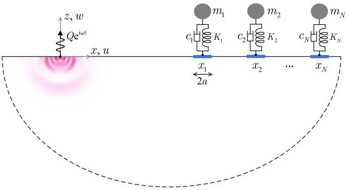
Figure 1: Schematic of Rayleigh wave interacting with resonators on an elastic half-space.

2.1 Surface harmonic load on a half-space

Let us consider a time-harmonic force per unit length $Q\mathrm{e}^{\mathrm{i}\omega t}$ applied normal to the free surface of an isotropic elastic medium. We resort to a two-dimensional (2D) plane-strain formulation in the $x-z$ plane, where the $x$-axis is directed along the wave propagation and the $z$-axis is perpendicular to the free surface (see Fig. 1). In absence of resonators, free stress boundary conditions ($\sigma_{zz}=\tau_{zx}=0$) characterize the elastic half-space along its whole surface except for the source location where:

$$\sigma_{zz}(x,z,t)=Q\delta(x)\mathrm{e}^{\mathrm{i}\omega t},\quad\tau_{zx}(x,z,t)=0,\quad\text{for}\quad x=0,\;z=0$$ (1)

Given the plane-strain conditions, the displacement vector lies in the plane $x-z$ with non-null components denoted as $\bm{u}(x,z,t)=[u,w]$. It is here convenient to use the Helmholtz decomposition $\bm{u}=\nabla\Phi+\nabla\times\bm{\Psi}$ and to express the displacement components as:

$$u=\frac{\partial\Phi}{\partial x}-\frac{\partial\Psi_{y}}{\partial z},\quad w=\frac{\partial\Phi}{\partial z}+\frac{\partial\Psi_{y}}{\partial x}$$ (2)

where $\Phi(x,z,t)$ is a scalar potential and $\Psi_{y}(x,z,t)$ is a component of the vector potential $\bm{\Psi}$.

Restricting our interest to the steady-state condition, the potentials assume the form:

$$\Phi(x,z,t)=\Phi(x,z)\mathrm{e}^{\mathrm{i}\omega t},\quad\Psi_{y}(x,z,t)=\Psi_{y}(x,z)\mathrm{e}^{\mathrm{i}\omega t}$$ (3)

and satisfy the wave equations [25]:

$$\nabla^{2}\Phi+k_{p}^{2}\Phi=0,\quad\nabla^{2}\Psi_{y}+k_{s}^{2}\Psi_{y}=0$$ (4)

in which $k_{p}$ and $k_{s}$ denote, respectively, the wave number of pressure and shear waves in the substrate, namely:

$$k_{p}=\frac{\omega}{c_{p}},\quad k_{s}=\frac{\omega}{c_{s}}$$ (5)

where:

$$c_{p}=\sqrt{\frac{\lambda+2\mu}{\rho}},\quad c_{s}=\sqrt{\frac{\mu}{\rho}}$$ (6)

are the pressure and shear wave velocities, respectively, $\lambda$ and $\mu$ the Lamé constants and $\rho$ the mass density of the substrate.

According to the Hooke’s law and employing the Helmholtz decomposition in Eq. (2), the in-plane components of the stress tensor $\bm{\sigma}$ can be expressed as function of the potentials:

$$\sigma_{zz}=-\mu\left[k_{s}^{2}\Phi+2\left(\frac{\partial^{2}\Phi}{\partial x^{2}}-\frac{\partial^{2}\Psi_{y}}{\partial x\partial z}\right)\right],\quad\tau_{zx}=-\mu\left[k_{s}^{2}\Psi_{y}-2\left(\frac{\partial^{2}\Phi}{\partial x\partial z}-\frac{\partial^{2}\Psi_{y}}{\partial z^{2}}\right)\right]$$ (7)

At this stage, we seek for the solutions of the wave Eqs. (4) by means of the Fourier transform along the $x$-direction:

$$\mathcal{F}\{\nabla^{2}\Phi+k_{p}^{2}\Phi\}=\frac{\partial^{2}\bar{\Phi}}{\partial z^{2}}-(k^{2}-k_{p}^{2})\bar{\Phi}=0,\quad\mathcal{F}\{\nabla^{2}\Psi_{y}+k_{s}^{2}\Psi_{y}\}=\frac{\partial^{2}\bar{\Psi}_{y}}{\partial z^{2}}-(k^{2}-k_{s}^{2})\bar{\Psi}_{y}=0$$ (8)

which admit general solutions of the form:

$$\bar{\Phi}(k,z)=A_{1}\mathrm{e}^{-pz}+B_{1}\mathrm{e}^{pz},\quad\bar{\Psi}_{y}(k,z)=A_{2}\mathrm{e}^{-qz}+B_{2}\mathrm{e}^{qz}$$ (9)

with:

$$p=\sqrt{k^{2}-k_{p}^{2}},\quad q=\sqrt{k^{2}-k_{s}^{2}}$$ (10)

and where the coefficients $A_{1}$ and $A_{2}$ in Eq. (9) must be equal to zero to avoid unbounded responses at increasing depth $z$. The remaining coefficients $B_{1}$ and $B_{2}$ are determined by imposing the boundary conditions.

Fourier transforming the stress components in Eq. (7), and making use of the boundary conditions in Eq. (1), lead to the following expressions:

$$(2k^{2}-k_{s}^{2})B_{1}+2\mathrm{i}kqB_{2}=Q/\mu$$ (11a)

$$-2\mathrm{i}kpB_{1}+(2k^{2}-k_{s}^{2})B_{2}=0$$ (11b)

Solutions of Eqs. (11a) and (11b) provide the coefficients:

$$B_{1}=\frac{Q}{\mu}\frac{(2k^{2}-k_{s}^{2})}{R(k)},\quad B_{2}=\frac{Q}{\mu}\frac{2\mathrm{i}kp}{R(k)}$$ (12)

where $R(k)$ denotes the so-called Rayleigh function:

$$R(k)\equiv(2k^{2}-k_{s}^{2})^{2}-4k^{2}pq$$ (13)

The inverse Fourier transform of Eq. (9) provides the expression of the potentials in the plane $x-z$:

$$\Phi(x,z)=\mathcal{F}^{-1}\{\bar{\Phi}\}=\frac{Q}{2\pi\mu}\int_{-\infty}^{\infty}\frac{2k^{2}-k_{s}^{2}}{R(k)}\mathrm{e}^{pz+\mathrm{i}kx}\,\mathrm{d}k$$ (14a)

$$\Psi_{y}(x,z)=\mathcal{F}^{-1}\{\bar{\Psi}_{y}\}=\frac{Q}{2\pi\mu}\int_{-\infty}^{\infty}\frac{2\mathrm{i}kp}{R(k)}\mathrm{e}^{qz+\mathrm{i}kx}\,\mathrm{d}k$$ (14b)

At last, by substituting Eqs. (14a) and (14b) into Eq. (2), the displacement components of the wavefield induced by the time-harmonic line load are obtained as:

$$u^{(f)}(x,z)=\frac{\mathrm{i}Q}{2\pi\mu}\int_{-\infty}^{\infty}\frac{k(2k^{2}-k_{s}^{2})\mathrm{e}^{pz}-2kpq\mathrm{e}^{qz}}{R(k)}\mathrm{e}^{\mathrm{i}kx}\,\mathrm{d}k$$ (15a)

$$w^{(f)}(x,z)=\frac{Q}{2\pi\mu}\int_{-\infty}^{\infty}\frac{p(2k^{2}-k_{s}^{2})\mathrm{e}^{pz}-2k^{2}p\mathrm{e}^{qz}}{R(k)}\mathrm{e}^{\mathrm{i}kx}\,\mathrm{d}k$$ (15b)

where the superscript ($f$) is used to label these displacement components of the free field (no resonators). From Eqs. (15a) and (15b) the free field displacement components at $z=0$ can be expressed as [1]:

$$u^{(f)}(x,0)=\frac{\mathrm{i}Q}{2\pi\mu}\int_{-\infty}^{\infty}\frac{k(2k^{2}-k_{s}^{2}-2pq)}{R(k)}\mathrm{e}^{\mathrm{i}kx}\,\mathrm{d}k$$ (16a)

$$w^{(f)}(x,0)=-\frac{Q}{2\pi\mu}\int_{-\infty}^{\infty}\frac{k_{s}^{2}p}{R(k)}\mathrm{e}^{\mathrm{i}kx}\,\mathrm{d}k$$ (16b)

2.2 Dynamics of surface resonators

We now consider the steady-state dynamics of mass-spring-dashpot resonators located atop an elastic half-space under harmonic motion. The set $\mathcal{O}=\{x_{1},x_{2},\cdots,x_{N}\mid N\in\mathbb{Z}^{+}\}\subset\mathbb{R}$ is introduced to collect the $x$-coordinate of the resonators. For each resonator we identify a footprint area $S$ with a length $2a$ along the $x$-direction.

The dynamic equilibrium equation of each resonator reads:

$$m_{n}\ddot{W_{n}}+c_{n}(\dot{W_{n}}-\dot{\tilde{w}}(x_{n},0))+K_{n}(W_{n}-\tilde{w}(x_{n},0))=0\quad\text{for}\quad x_{n}\in\mathcal{O}$$ (17)

where $m_{n}$, $c_{n}$ and $K_{n}$ are the $n$-th resonator mass, viscous damping coefficient and spring stiffness, $W_{n}$ is the absolute vertical displacement of the $n$-th mass, and $\tilde{w}(x_{n},0)$ is the average vertical displacement of the resonator footprint:

$$\tilde{w}(x_{n},0)=\frac{1}{2a}\int_{x_{n}-a}^{x_{n}+a}w(x,0)\,\mathrm{d}x\quad\text{for}\quad x_{n}\in\mathcal{O}$$ (18)

The use of an average base displacement is motivated by both physical and mathematical arguments. From a physical point, the average displacement represents the mean motion at the finite-size base of the oscillator. Mathematically, it allows to eliminate the divergence of the Green’s function at the origin.

According to Eq. (18), the absolute vertical displacement of the generic $n$-th resonator excited by a harmonic base motion $\tilde{w}(x_{n},0)$ of circular frequency $\omega$ reads:

$$W_{n}=\frac{m_{n}\omega_{rn}^{2}+\mathrm{i}\omega c_{n}}{m_{n}(\omega_{rn}^{2}-\omega^{2})+\mathrm{i}\omega c_{n}}\tilde{w}(x_{n},0)\equiv T_{Rn}\tilde{w}(x_{n},0)\quad\text{for}\quad x_{n}\in\mathcal{O}$$ (19)

where $T_{Rn}$ denotes the so-called transmissibility [26] of a damped resonator, and where $\omega_{rn}=\sqrt{K_{n}/m_{n}}$ is the angular resonant frequency of the $n$-th resonator. Accordingly, the normal force applied by the resonator to the substrate can be written as:

$$F_{n}=m_{n}\omega^{2}W_{n}=\frac{m_{n}\omega^{2}(m_{n}\omega_{rn}^{2}+\mathrm{i}\omega c_{n})}{m_{n}(\omega_{rn}^{2}-\omega^{2})+\mathrm{i}\omega c_{n}}\tilde{w}(x_{n},0)\equiv\Omega_{n}\tilde{w}(x_{n},0)\quad\text{for}\quad x_{n}\in\mathcal{O}$$ (20)

and the uniform stress exerted by each resonator over the contact area reads:

$$\sigma_{zz}(x,0)=\frac{F_{n}}{S}=\frac{\Omega_{n}\tilde{w}(x_{n},0)}{2a},\quad\tau_{zx}(x,0)=0,\quad\text{for}\quad x\in(x_{n}-a,x_{n}+a),\;x_{n}\in\mathcal{O}$$ (21)

These harmonic normal stresses behave as sources of additional wavefields in the half-space and interact with the free field generated by the source. The nature and implication of this interaction is described in the next section.

2.3 Surface resonators coupled to the half-space

As anticipated in the previous section, the resonators excited by a harmonic base motion generate additional wavefields in the half-space. We label the $j$-th resonator-induced wavefield $\bm{u}_{j}^{(s)}(x,z)$, where the superscript $(s)$ is used to denote scattered field, so that the total displacement field of the coupled problem can be written as:

$$\bm{u}(x,z)=\bm{u}^{(f)}(x,z)+\sum_{j=1}^{N}\bm{u}_{j}^{(s)}(x,z)\equiv\bm{u}^{(f)}(x,z)+\bm{u}^{(s)}(x,z)$$ (22)

where $\bm{u}^{(s)}(x,z)$ is the total wavefield. The free wavefield $\bm{u}^{(f)}(x,z)$, except for the point of application of the harmonic force ($x=0$), is characterized by null stress components at the surface:

$$\sigma_{zz}^{(f)}(x,0)=\tau_{zx}^{(f)}(x,0)=0\quad\text{for}\quad x\in\mathbb{R}\setminus\{0\}$$ (23)

hence, the stress at each resonator footprint depends only on the scattered wavefield, namely:

$$\sigma_{zz}(x,0)=\sigma_{zz}^{(f)}(x,0)+\sigma_{zz}^{(s)}(x,0)=\sigma_{zz}^{(s)}(x,0)\quad\text{for}\quad x\in(x_{n}-a,x_{n}+a),\;x_{n}\in\mathcal{O}$$ (24a)

$$\tau_{zx}(x,0)=\tau_{zx}^{(f)}(x,0)+\tau_{zx}^{(s)}(x,0)=0\quad\text{for}\quad x\in(x_{n}-a,x_{n}+a),\;x_{n}\in\mathcal{O}$$ (24b)

In force of Eq. (21) and Eq. (22), the scattered normal stress at the resonator footprint in Eq. (24a) can be written as:

$$\sigma_{zz}^{(s)}(x,0)=\frac{\Omega_{n}\tilde{w}(x_{n},0)}{2a}=\frac{\Omega_{n}[\tilde{w}^{(f)}(x_{n},0)+\tilde{w}^{(s)}(x_{n},0)]}{2a}\quad\text{for}\quad x\in(x_{n}-a,x_{n}+a),\;x_{n}\in\mathcal{O}$$ (25)

where the average free-field vertical displacement $\tilde{w}^{(f)}(x_{n},0)$ at the footprint of the $n$-th resonator can be obtained exploiting Eq. (15b) as:

$$\tilde{w}^{(f)}(x_{n},0)=\frac{1}{2a}\frac{-Q}{2\pi\mu}\int_{x_{n}-a}^{x_{n}+a}\int_{-\infty}^{\infty}\frac{k_{s}^{2}p}{R(k)}\mathrm{e}^{\mathrm{i}kx}\,\mathrm{d}x\mathrm{d}k=\frac{-Q}{2\pi\mu}\int_{-\infty}^{\infty}\frac{k_{s}^{2}p}{R(k)}\frac{\sin(ka)}{ka}\mathrm{e}^{\mathrm{i}kx_{n}}\,\mathrm{d}k\quad\text{for}\quad x_{n}\in\mathcal{O}$$ (26)

The average scattered field $\tilde{w}^{(s)}(x_{n},0)$ can be instead obtained as described in the following. First Eqs. (15a) and (15b) are used as Green’s functions to express the displacement components of the scattered field $\bm{u}_{j}^{(s)}(x,z)$ generated by the normal stress exerted by the $j$-th resonator:

$$\begin{split}u_{j}^{(s)}(x,z)&=\mathrm{i}\int_{x_{j}-a}^{x_{j}+a}\frac{\sigma_{zz}^{(s)}(\eta,0)}{2\pi\mu}\int_{-\infty}^{\infty}\frac{k(2k^{2}-k_{s}^{2})\mathrm{e}^{pz}-2kpq\mathrm{e}^{qz}}{R(k)}\mathrm{e}^{\mathrm{i}k(x-\eta)}\,\mathrm{d}\eta\mathrm{d}k\\ &=\frac{\mathrm{i}\Omega_{j}[\tilde{w}^{(f)}(x_{j},0)+\tilde{w}^{(s)}(x_{j},0)]}{2\pi\mu}\int_{-\infty}^{\infty}\frac{k(2k^{2}-k_{s}^{2})\mathrm{e}^{pz}-2kpq\mathrm{e}^{qz}}{R(k)}\frac{\sin(ka)}{ka}\mathrm{e}^{\mathrm{i}k(x-x_{j})}\,\mathrm{d}k\quad\text{for}\quad x_{j}\in\mathcal{O}\end{split}$$ (27a)

$$\begin{split}w_{j}^{(s)}(x,z)&=\int_{x_{j}-a}^{x_{j}+a}\frac{\sigma_{zz}^{(s)}(\eta,0)}{2\pi\mu}\int_{-\infty}^{\infty}\frac{p(2k^{2}-k_{s}^{2})\mathrm{e}^{pz}-2k^{2}p\mathrm{e}^{qz}}{R(k)}\mathrm{e}^{\mathrm{i}k(x-\eta)}\,\mathrm{d}\eta\mathrm{d}k\\ &=\frac{\Omega_{j}[\tilde{w}^{(f)}(x_{j},0)+\tilde{w}^{(s)}(x_{j},0)]}{2\pi\mu}\int_{-\infty}^{\infty}\frac{p(2k^{2}-k_{s}^{2})\mathrm{e}^{pz}-2k^{2}p\mathrm{e}^{qz}}{R(k)}\frac{\sin(ka)}{ka}\mathrm{e}^{\mathrm{i}k(x-x_{j})}\,\mathrm{d}k\quad\text{for}\quad x_{j}\in\mathcal{O}\end{split}$$ (27b)

Note that the calculation of each scattered wavefield $u_{j}^{(s)}(x,z)$, and $w_{j}^{(s)}(x,z)$, as per Eqs. (27a) and (27b), requires only the knowledge of the average vertical displacement, free $\tilde{w}^{(f)}(x_{j},0)$ and scattered $\tilde{w}^{(s)}(x_{j},0)$, at the contact points $x_{j}\in\mathcal{O}$.

Since the free field component $\tilde{w}^{(f)}(x_{j},0)$ is known from Eq. (26), the only left unknowns in Eqs. 27a and 27b are the vertical scattered displacements $\tilde{w}^{(s)}(x_{j},0)$. To calculate them, we expand the average vertical scattered displacement field at the contact points $x_{n}$ according to Eq. (22):

$$\tilde{w}^{(s)}(x_{n},0)=\sum_{j=1}^{N}\tilde{w}_{j}^{(s)}(x_{n},0)\quad\text{for}\quad n=1,2,\cdots,N$$ (28)

which can be equivalently rewritten as:

$$\begin{cases}\tilde{w}^{(s)}(x_{1},0)=\tilde{w}_{1}^{(s)}(x_{1},0)+\tilde{w}_{2}^{(s)}(x_{1},0)+\cdots+\tilde{w}_{N}^{(s)}(x_{1},0)\\ \tilde{w}^{(s)}(x_{2},0)=\tilde{w}_{1}^{(s)}(x_{2},0)+\tilde{w}_{2}^{(s)}(x_{2},0)+\cdots+\tilde{w}_{N}^{(s)}(x_{2},0)\\ \quad\quad\vdots\\ \tilde{w}^{(s)}(x_{N},0)=\tilde{w}_{1}^{(s)}(x_{N},0)+\tilde{w}_{2}^{(s)}(x_{N},0)+\cdots+\tilde{w}_{N}^{(s)}(x_{N},0)\\ \end{cases}$$ (29)

Then, we substitute Eq. (27b) into Eq. (29) and obtain the following equations:

$$\begin{cases}\tilde{w}^{(s)}(x_{1},0)=\beta_{11}[\tilde{w}^{(f)}(x_{1},0)+\tilde{w}^{(s)}(x_{1},0)]+\beta_{12}[\tilde{w}^{(f)}(x_{2},0)+\tilde{w}^{(s)}(x_{2},0)]+\cdots+\beta_{1N}[\tilde{w}^{(f)}(x_{N},0)+\tilde{w}^{(s)}(x_{N},0)]\\ \tilde{w}^{(s)}(x_{2},0)=\beta_{21}[\tilde{w}^{(f)}(x_{1},0)+\tilde{w}^{(s)}(x_{1},0)]+\beta_{22}[\tilde{w}^{(f)}(x_{2},0)+\tilde{w}^{(s)}(x_{2},0)]+\cdots+\beta_{2N}[\tilde{w}^{(f)}(x_{N},0)+\tilde{w}^{(s)}(x_{N},0)]\\ \quad\quad\vdots\\ \tilde{w}^{(s)}(x_{N},0)=\beta_{N1}[\tilde{w}^{(f)}(x_{1},0)+\tilde{w}^{(s)}(x_{1},0)]+\beta_{N2}[\tilde{w}^{(f)}(x_{2},0)+\tilde{w}^{(s)}(x_{2},0)]+\cdots+\beta_{NN}[\tilde{w}^{(f)}(x_{N},0)+\tilde{w}^{(s)}(x_{N},0)]\\ \end{cases}$$ (30)

where:

$$\begin{split}\beta_{nj}&=\frac{-\Omega_{j}}{2\pi\mu}\frac{1}{2a}\int_{-\infty}^{\infty}\frac{k_{s}^{2}p}{R(k)}\frac{\sin(ka)}{ka}\,\mathrm{d}k\int_{x_{n}-a}^{x_{n}+a}\mathrm{e}^{\mathrm{i}k(x-x_{j})}\,\mathrm{d}x\\ &=\frac{-\Omega_{j}}{2\pi\mu}\int_{-\infty}^{\infty}\frac{k_{s}^{2}p}{R(k)}\frac{\sin^{2}(ka)}{(ka)^{2}}\mathrm{e}^{\mathrm{i}k(x_{n}-x_{j})}\,\mathrm{d}k\quad\text{for}\quad n,j=1,2,\cdots,N\end{split}$$ (31)

For simplicity, we express Eq. (30) in matrix form as:

$$\bm{A}\bm{x}=\bm{b}$$ (32)

where the corresponding coefficients are:

$$\bm{A}=\left[\begin{array}[]{cccc}{(1-\beta_{11})}&{-\beta_{12}}&{\cdots}&{-\beta_{1N}}\\ {-\beta_{21}}&{(1-\beta_{22})}&{\cdots}&{-\beta_{2N}}\\ {\vdots}&{\vdots}&{\ddots}&{\vdots}\\ {-\beta_{N1}}&{-\beta_{N2}}&{\cdots}&{(1-\beta_{NN})}\\ \end{array}\right]\in\mathbb{C}^{N\times N}$$ (33a)

$$\bm{x}=\left[\begin{array}[]{c}{\tilde{w}^{(s)}(x_{1},0)}\\ {\tilde{w}^{(s)}(x_{2},0)}\\ \vdots\\ {\tilde{w}^{(s)}(x_{N},0)}\\ \end{array}\right]\in\mathbb{C}^{N\times 1},\quad\bm{b}=\left[\begin{array}[]{c}{\beta_{11}\tilde{w}^{(f)}(x_{1},0)+\beta_{12}\tilde{w}^{(f)}(x_{2},0)+\cdots+\beta_{1N}\tilde{w}^{(f)}(x_{N},0)}\\ {\beta_{21}\tilde{w}^{(f)}(x_{1},0)+\beta_{22}\tilde{w}^{(f)}(x_{2},0)+\cdots+\beta_{2N}\tilde{w}^{(f)}(x_{N},0)}\\ \vdots\\ {\beta_{N1}\tilde{w}^{(f)}(x_{1},0)+\beta_{N2}\tilde{w}^{(f)}(x_{2},0)+\cdots+\beta_{NN}\tilde{w}^{(f)}(x_{N},0)}\\ \end{array}\right]\in\mathbb{C}^{N\times 1}$$ (33b)

The solution of Eq. (32) provides the sought average vertical displacement components of the scattered field at the resonator footprint locations $x_{n}$. When the matrix $\bm{A}$ has a nonzero determinant, the system in Eq. (32) has a unique solution $\bm{x}$ with components:

$$\tilde{w}^{(s)}(x_{n},0)=(\bm{A}^{-1}\bm{b})_{n}\quad\text{for}\quad n=1,2,\cdots,N$$ (34)

At this stage, by substituting Eq. (34) into Eqs. (27a), (27b), we can obtain the $j$-th scattered field components $u_{j}^{(s)}(x,z)$ and $w_{j}^{(s)}(x,z)$ at any point of the $x-z$ plane. The total wavefield is then obtained as the summation of the free and scattered fields:

$$u(x,z)=u^{(f)}(x,z)+u^{(s)}(x,z)=u^{(f)}(x,z)+\sum_{j=1}^{N}u_{j}^{(s)}(x,z)$$ (35a)

$$w(x,z)=w^{(f)}(x,z)+w^{(s)}(x,z)=w^{(f)}(x,z)+\sum_{j=1}^{N}w_{j}^{(s)}(x,z)$$ (35b)

Equations (35a) and (35b) can be rewritten in integral form as follows:

$$\begin{split}u(x,z)&=\frac{\mathrm{i}Q}{2\pi\mu}\int_{-\infty}^{\infty}\frac{k(2k^{2}-k_{s}^{2})\mathrm{e}^{pz}-2kpq\mathrm{e}^{qz}}{R(k)}\mathrm{e}^{\mathrm{i}kx}\,\mathrm{d}k\\ &+\frac{\mathrm{i}}{2\pi\mu}\sum_{j=1}^{N}\Omega_{j}\left[\frac{-Q}{2\pi\mu}\int_{-\infty}^{\infty}\frac{k_{s}^{2}p}{R(k)}\frac{\sin(ka)}{ka}\mathrm{e}^{\mathrm{i}kx_{j}}\,\mathrm{d}k+(\bm{A}^{-1}\bm{b})_{j}\right]\int_{-\infty}^{\infty}\frac{k(2k^{2}-k_{s}^{2})\mathrm{e}^{pz}-2kpq\mathrm{e}^{qz}}{R(k)}\frac{\sin(ka)}{ka}\mathrm{e}^{\mathrm{i}k(x-x_{j})}\,\mathrm{d}k\end{split}$$ (36)

$$\begin{split}w(x,z)&=\frac{Q}{2\pi\mu}\int_{-\infty}^{\infty}\frac{p(2k^{2}-k_{s}^{2})\mathrm{e}^{pz}-2k^{2}p\mathrm{e}^{qz}}{R(k)}\mathrm{e}^{\mathrm{i}kx}\,\mathrm{d}k\\ &+\frac{1}{2\pi\mu}\sum_{j=1}^{N}\Omega_{j}\left[\frac{-Q}{2\pi\mu}\int_{-\infty}^{\infty}\frac{k_{s}^{2}p}{R(k)}\frac{\sin(ka)}{ka}\mathrm{e}^{\mathrm{i}kx_{j}}\,\mathrm{d}k+(\bm{A}^{-1}\bm{b})_{j}\right]\int_{-\infty}^{\infty}\frac{p(2k^{2}-k_{s}^{2})\mathrm{e}^{pz}-2k^{2}p\mathrm{e}^{qz}}{R(k)}\frac{\sin(ka)}{ka}\mathrm{e}^{\mathrm{i}k(x-x_{j})}\,\mathrm{d}k\end{split}$$ (37)

The above Eqs. (36) and (37) can be specified at the coordinate $z=0$ to obtain the surface displacement components:

$$\begin{split}u(x,0)&=\frac{\mathrm{i}Q}{2\pi\mu}\int_{-\infty}^{\infty}\frac{k(2k^{2}-k_{s}^{2}-2pq)}{R(k)}\mathrm{e}^{\mathrm{i}kx}\,\mathrm{d}k\\ &+\frac{\mathrm{i}}{2\pi\mu}\sum_{j=1}^{N}\Omega_{j}\left[\frac{-Q}{2\pi\mu}\int_{-\infty}^{\infty}\frac{k_{s}^{2}p}{R(k)}\frac{\sin(ka)}{ka}\mathrm{e}^{\mathrm{i}kx_{j}}\,\mathrm{d}k+(\bm{A}^{-1}\bm{b})_{j}\right]\int_{-\infty}^{\infty}\frac{k(2k^{2}-k_{s}^{2}-2pq)}{R(k)}\frac{\sin(ka)}{ka}\mathrm{e}^{\mathrm{i}k(x-x_{j})}\,\mathrm{d}k\end{split}$$ (38)

$$\begin{split}w(x,0)&=\frac{-Q}{2\pi\mu}\int_{-\infty}^{\infty}\frac{k_{s}^{2}p}{R(k)}\mathrm{e}^{\mathrm{i}kx}\,\mathrm{d}k\\ &-\frac{1}{2\pi\mu}\sum_{j=1}^{N}\Omega_{j}\left[\frac{-Q}{2\pi\mu}\int_{-\infty}^{\infty}\frac{k_{s}^{2}p}{R(k)}\frac{\sin(ka)}{ka}\mathrm{e}^{\mathrm{i}kx_{j}}\,\mathrm{d}k+(\bm{A}^{-1}\bm{b})_{j}\right]\int_{-\infty}^{\infty}\frac{k_{s}^{2}p}{R(k)}\frac{\sin(ka)}{ka}\mathrm{e}^{\mathrm{i}k(x-x_{j})}\,\mathrm{d}k\end{split}$$ (39)

The closed-form Eqs. (36), (37), (38), (39) are evaluated numerically via Gauss-Kronrod quadrature. In the next section we use the developed approach to predict the wavefield of half-spaces with different sets of resonators including uniform, graded and disordered arrays.

3 Case studies

In this section, we discuss the behavior of a single resonator, a couple of resonators, and a graded array of resonators placed atop an elastic half-space and excited by a far field source. Our aim is twofold: (i) to test and validate the accuracy of our formulation against a numerical (Finite Element) solution; (ii) to discuss the coupling between free and scattered wavefields for different mechanical parameters and layout of the resonators.

Before tackling these tasks, let us provide some useful parameters to facilitate our calculations and ease the further discussions:

• to generalize our conclusions, we introduce the dimensionless mass parameter $\hat{m}_{j}=m_{j}/(\rho S\lambda_{rj})$, with $\rho$ being the density of the half-space and $\lambda_{rj}=c_{R}/f_{rj}$ the Rayleigh wavelength at resonant frequency $f_{rj}$; this parameter compares the mass of the resonator to the mass of a portion of substrate under the resonator footprint area, with volume $V=S\times\lambda_{rj}$. Additionally, we introduce the parameter $\hat{d}_{mn}=d_{mn}/\lambda_{rj}=(x_{n}-x_{m})/\lambda_{rj}$ to denote the normalized distance between the $m$-th and $n$-th resonator.

• to account for wave energy dissipation, we assume a non-null damping ratio $\zeta$ for the resonator response and a non-null hysteretic damping $\xi$ for the elastic substrate. The damping coefficient of the $j$-th resonator is calculated as $c_{j}=2m_{j}\omega_{rj}\zeta$ [26], while the complex moduli of the substrate as $\lambda^{\prime}=\lambda(1+2\mathrm{i}\xi)$ and $\mu^{\prime}=\mu(1+2\mathrm{i}\xi)$ [27]; the introduction of damping in the system allows also to avoid numerical instabilities by removing the poles of the integrands in Eqs. (38, 39);

• to quantify the contribution of the resonators scattered field at the half-space surface ($z=0$), we introduce the following amplitude ratio ($A_{R}$) [28]:

  $$A_{R}=\frac{w(x,0)}{w^{(f)}(x,0)}=1+\frac{w^{(s)}(x,0)}{w^{(f)}(x,0)}$$ (40)

  and the normalized distance between the receiver and the first resonator $\hat{d}=d/\lambda_{r1}=(x-x_{1})/\lambda_{r1}$ where $A_{R}$ will be computed.

3.1 Single resonator scenario

We begin our investigation considering the case of a single surface oscillator. The resonator has a normalized mass $\hat{m}_{1}=1$, is located at a distance $x_{1}=6\lambda_{r1}$ from the harmonic source, and lies over a half-space characterized by the mechanical properties collected in Table 1.

The total wavefield generated by a harmonic source at $f=f_{r1}$, computed by using Eqs. (36) and (37), is shown in Fig. 2a in the domain $x=[4,8]\lambda_{r1}$, $z=[-2,0]\lambda_{r1}$. The analytically predicted wavefield is in excellent agreement with the one displayed in Fig. 2b, calculated with harmonic FE simulations (see A for details on the FE model). To quantify the effect of the resonator on the surface wavefield, we calculate and show in Fig. 2c the amplitude ratio $|A_{R}|$ for harmonic sources with frequencies $f=[0,3]f_{r1}$ at two positions, namely $\hat{d}=0.1$ (blue line), in the scattered near field, and at $\hat{d}=6$ (red line), in the scattered far field.

Table 1: Mechanical parameters of the resonators and the elastic half-space. The elastic parameters are taken from Ref. [29].

Parameter	Value
Line load amplitude, $Q$	$10^{6}$ N/m
First resonator frequency, $f_{r1}$	2 Hz
Footprint length of each resonator, $2a$	1 m
Damping ratio of resonators, $\zeta$	1$\%$
Mass density of substrate, $\rho$	1800 kg/m3
Young modulus of substrate, $E$	46 MPa
Poisson ratio of substrate, $\nu$	0.25
Hysteretic damping ratio of substrate, $\xi$	1$\%$

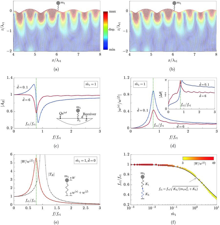
Figure 2: Rayleigh wave interaction with a single resonator on an elastic half-space ($\hat{m}_{1}=1$, $x_{1}=6\lambda_{r1}$). Total wavefield for a harmonic source at $f=f_{r1}$ computed using the (a) proposed analytical solution, (b) FE simulation. (c) Amplitude ratio $|A_{R}|$ in the near $\hat{d}=0.1$ (blue line) and far field $\hat{d}=6$ (red line). (d) Spectrum and phase of the scattered field vs. the free field. (e) Dynamic amplification factor of the resonator on a rigid (dashed line) and elastic substrate (red line). (f) Coupled frequency $f_{c1}$ vs. the mass of the resonator. For comparison, in (c), (d) and (e) we also provide the FE solutions denoted by dots.

In the near field response we observe a low-frequency region where the surface motion is amplified with respect to the free field, namely $|A_{R}|>1$, followed by a higher frequency region with a significant deamplification of the signal. The two regimes are separated by the frequency $f_{c1}$ which corresponds to the resonance of the oscillator coupled to the elastic substrate. In the far field the signal amplification disappears and we observe only a deamplification of the signal with a maximum drop occurring exactly at the coupled frequency $f_{c1}$.

To interpret the different responses observed near and far from the resonator, we expand the expression of $|A_{R}|$ given in Eq. (40) as:

$$|A_{R}|=\sqrt{1+\left|\frac{w^{(s)}}{w^{(f)}}\right|^{2}+2\mathrm{Re}\left(\frac{w^{(s)}}{w^{(f)}}\right)}=\sqrt{1+\left|\frac{w^{(s)}}{w^{(f)}}\right|^{2}+2\left|\frac{w^{(s)}}{w^{(f)}}\right|\cos(\Delta\theta)}$$ (41)

where $\Delta\theta$ is the relative phase between the scattered and free vertical displacements, namely, $w^{(s)}/w^{(f)}$.

According to the Eq. (41), both the amplitude and the relative phase of the scattered field play a role in the amplitude ratio $|A_{R}|$: the scattered field amplitude shows a similar trend both in the near and in the far field and reaches its peak exactly at the coupled frequency $f_{c1}$ (see Fig. 2d); conversely, the relative phase $\Delta\theta$ significantly changes depending on the receiver location. In the near field, around the coupling frequency, the relative phase (see inset in Fig. 2d) shows that the scattered and free responses are approximately orthogonal. Hence, the contribution of the scattered waves to the value of $|A_{R}|$ is negligible. Conversely, in the far field, scattered and free responses are out-of-phase, leading to destructive interference between the two wavefields and to a minimum value of the amplification ratio $|A_{R}|$.

Let us now investigate in more detail the variation of the coupled frequency $f_{c1}$ with respect to the mechanical parameters of the system, namely substrate and oscillator. To this purpose, we calculate the absolute vertical displacement $W$ of a resonator located on the half-space surface at distance $d=0$ from the source and compare its response to the one of an identical resonator placed on a rigid substrate. The two resonators vertical responses, normalized with respect to the relative base displacements, are plotted in Fig. 2e. As expected, the response of the resonator on a rigid substrate provides the transmissibility factor $|T_{R}|$ (dashed line), whereas the maximum amplitude response of the resonator lying on the half-space (red continuous line) does not occur at its natural frequency $f_{r1}$ but is shifted towards the coupled resonant frequency $f_{c1}$. This frequency shift can be predicted utilizing a lumped-mass model, in which the contribution of the half-space is lumped in the additional stiffness $K_{h}$ (see schematic in Fig. 2f). Hence, the coupled frequency can be calculated as:

$$f_{c1}=f_{r1}\sqrt{\frac{K_{h}}{m_{1}\omega_{r1}^{2}+K_{h}}}$$ (42)

where the equivalent substrate stiffness $K_{h}$ can be estimated from Eq. (27b) by considering the averaged stress over the contact area ($z=0$) and a null source-response distance ($x=x_{j}$):

$$\frac{1}{K_{h}}=\frac{-1}{2\pi\mu}\int_{-\infty}^{\infty}\frac{k_{s}^{2}p}{R(k)}\frac{\sin^{2}(ka)}{(ka)^{2}}\,\mathrm{d}k$$ (43)

Note that the integral in Eq. (43) is frequency dependent, so strictly speaking the coupling frequency $f_{c1}$ in Eq. (42) is frequency dependent too. As an approximation, here we calculate the value of $K_{h}$ at $f=f_{r1}$ and use it to predict the value of $f_{c1}$ for different resonator mass.

The value of the coupled frequency vs. the resonator mass as predicted from Eq. (42) is plotted in Fig. 2f as a continuous black line. The prediction agrees well with the frequency values at which the response of the different resonators reach its maximum amplitude as calculated from Eq. (19) (marked in Fig. 2f by colored circles). In particular, the color of the circles shows the value of the amplification factor ($W/w^{(f)}$) at resonance, and highlights that a change of mass produces a change in the effective quality factor of the resonator too. To conclude this section, we remark that all these results have been validated with FE models (see black dots superimposed onto all the curves in Figs. 2c,d,e).

3.2 Two resonators scenario

Studies on the dynamics of coupled oscillators on elastic supports are receiving renovate attention both in the geophysical context, to assess the response of close buildings and their influence on ground vibrations, and in the design of SAW devices, where micro/nano resonators are proposed for application in classical and quantum information processing [30]. In what follows, we show how our analytical formulation allows to properly analyze the mutual interaction between close resonators and to quantify its effects on the half-space and resonator responses.

We begin our investigation considering two identical resonators, with parameters given in Table 1 and with a relative spacing $d_{12}=0.1\lambda_{r1}$, excited by a far field ($x_{1}=6\lambda_{r1}$) harmonic source. We calculate the amplitude ratio $|A_{R}|$ for a receiver located at $\hat{d}=6$ from the first resonator. The presence of two oscillators atop the half-space leads to a significant reduction in the amplitude ratio which shows its minimum value at a frequency different from the resonator coupled frequency ($f_{c1}=f_{c2}$). We remark that the system response cannot be predicted from the simple superposition of the single resonator scenarios, which would neglect the cross-coupling interaction between the two resonators (see the $|A_{R}|$ of each single resonator scenario (blue lines) in Fig. 3a). To investigate further the coupling between the responses of the resonators, we expand the expression of the amplitude ratio as:

$$|A_{R}|=\sqrt{1+\left|\frac{w_{1}^{(s)}}{w^{(f)}}\right|^{2}+\left|\frac{w_{2}^{(s)}}{w^{(f)}}\right|^{2}+2\left|\frac{w_{1}^{(s)}}{w^{(f)}}\right|\cos(\Delta\theta_{1})+2\left|\frac{w_{2}^{(s)}}{w^{(f)}}\right|\cos(\Delta\theta_{2})+2\left|\frac{w_{1}^{(s)}}{w^{(f)}}\right|\left|\frac{w_{2}^{(s)}}{w^{(f)}}\right|\cos(\Delta\theta_{2}-\Delta\theta_{1})}$$ (44)

where $\Delta\theta_{1}$ and $\Delta\theta_{2}$ denote the phase of $w_{1}^{(s)}/w^{(f)}$ and $w_{2}^{(s)}/w^{(f)}$, respectively. The above equation clearly highlights the presence of the cross-coupling contribution, namely, the last term in Eq. (44), in addition to the independent contributions of each resonator.

This mutual interaction modifies also the resonators responses, as highlighted by Fig. 3b where the uncoupled and coupled oscillators amplification factors are shown. In particular, by looking at the maximum of the $|A_{R}|$ factor, one can observe a shift in the resonance of both oscillators. Additionally, the first resonator shows a characteristic “frequency splitting” behavior, recently observed experimentally in couples of micropillars attached to an elastic substrate [30].

An effective mutual interaction requires resonators with similar (possibly identical) resonance frequencies located at a relatively short distance. That is because the scattered fields are maximized at the coupled resonance frequencies and in the near fields of the resonators, as shown in Fig. 2d for a single resonator. To evidence this effect, let us consider a configuration of two resonators with different natural frequencies, e.g., $f_{r2}=2f_{r1}$, keeping the other parameters unchanged. Fig. 3c shows the amplitude ratio at $\hat{d}=6$. The reader can appreciate that the system response is now simply the envelope, namely the superposition of the two single case scenarios. Similarly, the amplification factors of the two resonators, reported in Fig. 3d, confirm that no significant shift occurs in the coupled frequencies of each resonator.

We remark that the extraction of these features is eased by our analytical framework which allows to investigate and distinguish the contribution of each scattered field to the total response.

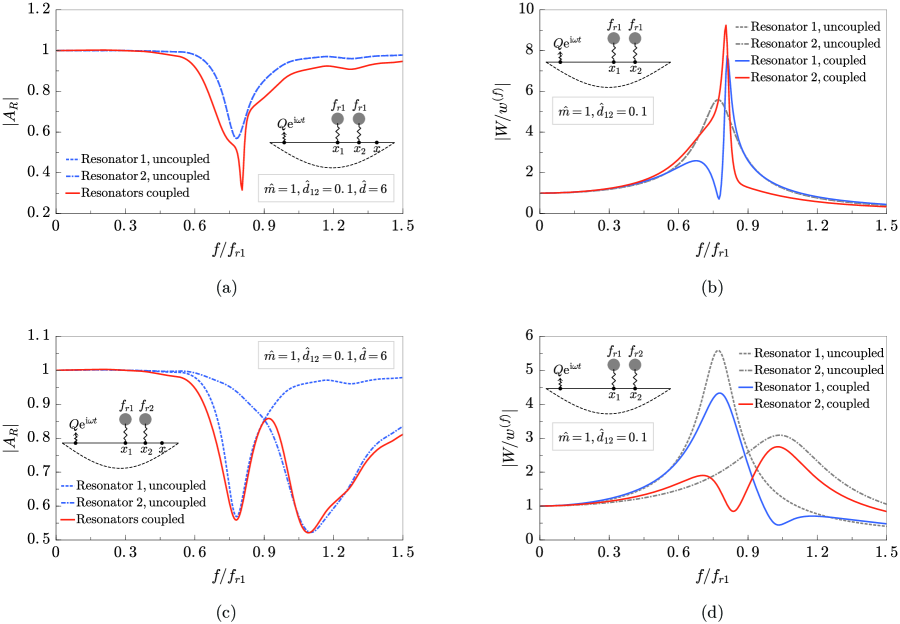
Figure 3: Rayleigh wave interaction with two resonators on an elastic half-space ($\hat{m}_{1}=\hat{m}_{2}=1,x_{1}=6\lambda_{r1},d_{12}=0.1\lambda_{r1}$). (a) Amplitude ratio $|A_{R}|$ computed at $\hat{d}=6$ for two identical resonators ($f_{r2}=f_{r1}$). (b) Uncoupled and coupled amplification factors for two identical resonators ($f_{r2}=f_{r1}$). (c) Amplitude ratio $|A_{R}|$ computed at $\hat{d}=6$ for two different resonators ($f_{r2}=2f_{r1}$). (d) Uncoupled and coupled amplification factors for two different resonators ($f_{r2}=2f_{r1}$).

3.3 Cluster of resonators

So far we have gained some physical insights into the behavior of single and coupled oscillators lying over an elastic substrate. When the number of resonators increases to form a cluster, or a so-called metasurface, the propagation of surface waves in the elastic substrate can be characterized by intriguing phenomena, such as surface-to-bulk wave conversions (from classical [13] and Umklapp scattering [16]) and wave localization (via classical [23] and topological rainbow trapping [24]). Although the extraction of the dispersive properties of such graded clusters can be typically inferred from analytical models developed for infinite regular arrays [14], the evaluation of the related wavefields require the use of numerical schemes. In what follows, we will show that our analytical framework can properly capture these phenomena.

We begin by considering an array of 40 identical resonators ($\hat{m}_{j}=0.5,f_{rj}=f_{r1}$), arranged periodically with a lattice spacing $0.1\lambda_{r1}$ (see Fig. 4a). Similar arrays have been analyzed to assess the surface wave filtering capabilities of a periodic metasurface [23, 18]. For such a configuration, we expect the existence of a band gap in a narrow frequency region above the oscillator resonance and the occurrence of surface-to-shear wave conversion.

To visualize this phenomenon, we consider an incident Rayleigh wave with frequency $f=1.1f_{r1}$, namely in the metasurface band gap, which is excited by the harmonic source $Q\mathrm{e}^{\mathrm{i}\omega t}$ sufficiently far away from the metasurface ($x_{1}=6\lambda_{r1}$). The displacement wavefield is displayed in Fig. 4a and shows how the incident Rayleigh wave is converted into a downward propagating shear wave.

The same wave-conversion phenomenon can be extended over a broader frequency range by utilizing a series of resonators with a graded variation of frequency along the array [23]. To achieve this purpose, we model an array of 40 resonators ($\hat{m}_{j}=0.5$) with resonant frequencies linearly increasing along the array with a step $\Delta f_{r}=0.05f_{r1}$, for an overall working bandwidth between $f_{r1}$ and 3$f_{r1}$. Alike the periodic metasurface previously discussed, we set a constant spacing between the resonators. Indeed, this graded configuration, also known in the literature as metawedge [23], supports both a mode conversion and a wave localization, depending on the direction of the incoming excitation. These two distinct wavefields, as calculated using our analytical framework, are shown respectively in Figs. 4b and 4c.

As last example, we calculate the wavefield of a disordered metasurface, constructed by randomly changing the order of resonators considered in the discussed metawedge. The investigation of such a non-periodic resonant system is attracting increasing interest in the research community as a design strategy to enlarge the filtering bandwidth of metamaterials [31, 32]. Note that a random configuration can be easily modeled using the proposed analytical approach which allows to set frequency and location of the resonating scatters at will. In Fig. 4d the reader can appreciate the related wavefield for an incident Rayleigh wave at $f=1.1f_{r1}$.

We also provide a comparison of the amplitude ratio $|A_{R}|$ calculated at $\hat{d}=6$ in the frequency range $f=[0,3]f_{r1}$. The result is shown in Fig. 4e and highlights that the disordered metasurface provides similar filtering performance to the two analyzed graded systems.

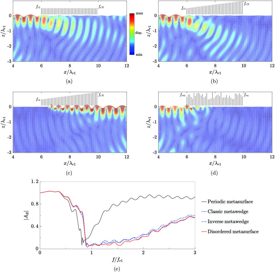
Figure 4: Rayleigh wave interaction with finite-size metasurfaces ($N=40$) on an elastic half-space ($\hat{m}=0.5$, resonator spacing $0.1\lambda_{r1}$, incident frequency $f=1.1f_{r1}$). Calculated wave field for: (a) a periodic metasurface. (b) an inverse metawedge. (c) a classical metawedge. (d) a disordered metasurface. In the schematics the length of the resonators represent the value of the related natural frequencies. (e) Amplitude ratio $|A_{R}|$ computed at $\hat{d}=6$ in the frequency range $f=[0,3]f_{r1}$ of the four considered cases.

4 Conclusions

This work proposes an analytical formulation to model and study the interaction of vertically polarized elastic waves with surface resonators. In particular, we have exploited the Green’s functions of the canonical Lamb’s problem to setup a coupled problem between the incident field generated by the source and the scattered wavefields generated by a set of resonators placed atop the half-space. The formulation can handle an arbitrary number of resonators arranged on the surface of the half-space in a generic configuration. The capabilities of the developed methodology have been discussed by modeling the dynamics of a single, a couple and a cluster of resonators arranged over an isotropic homogeneous half-space, and have been validated against finite element simulations.

The method allows to capture the frequency shift of a resonator coupled to the elastic substrate, the mutual interaction between a couple of close resonators in terms of frequency splitting and amplitude variation and the collective response of arrays of resonators, e.g., metasurfaces interacting with Rayleigh waves. Future research efforts will be devoted to extend the methodology to a 3D scenario and exploit its capability to design SAW devices, waveguides and interpret the dynamics of a cluster of buildings interacting with seismic waves and urban vibrations.

CRediT authorship contribution statement

Xingbo Pu: Conceptualization, Methodology, Investigation, Software, Data curation, Writing - original draft. Antonio Palermo: Conceptualization, Investigation, Validation, Writing - review & editing, Co-supervision. Alessandro Marzani: Conceptualization, Investigation, Writing - review & editing, Supervision, Funding acquisition.

Declaration of competing interest

The authors declare that they have no conflict of interest.

Appendix A Details on the FE model

In this Appendix, we provide details of the FE model (see Fig. 1) used to validate our analytical solutions in Section 3.1. First, to simulate the uniform vertical force imposed on the footprint, the mass-dashpot-spring oscillator is discretized as an ensemble of 11 truss elements, namely the truss spacing $0.2a\ll\lambda_{r}$. This procedure results in each point mass $m_{p}=m/11$, and the Young modulus of each truss $E_{t}=(m_{p}\omega_{r}^{2}+\mathrm{i}\omega c)/A_{t}$, where $A_{t}$ is the cross-sectional area of a truss. The incident Rayleigh wave is excited by the harmonic load with amplitude $Q$ at a sufficient distance ($6\lambda_{r}$) from the oscillator. To model the elastic half-space and to avoid unnecessary reflections, we add Perfectly Matched Layers (PMLs) to the vertical and bottom edges.

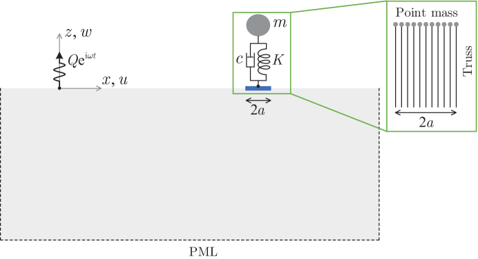
Figure 1: Schematic of FE model.

References

- [1] H. Lamb, I. on the propagation of tremors over the surface of an elastic solid, Philosophical Transactions of the Royal Society of London. Series A, Containing papers of a mathematical or physical character 203 (359-371) (1904) 1–42. doi:10.1098/rsta.1904.0013.
- [2] J. Luco, F. De Barros, Dynamic displacements and stresses in the vicinity of a cylindrical cavity embedded in a half-space, Earthquake engineering & structural dynamics 23 (3) (1994) 321–340. doi:10.1002/eqe.4290230307.
- [3] Y. Tanaka, S.-i. Tamura, Surface acoustic waves in two-dimensional periodic elastic structures, Physical Review B 58 (12) (1998) 7958. doi:10.1103/PhysRevB.58.7958.
- [4] I. Malfanti, A. Taschin, P. Bartolini, B. Bonello, R. Torre, Propagation of acoustic surface waves on a phononic surface investigated by transient reflecting grating spectroscopy, Journal of the Mechanics and Physics of Solids 59 (11) (2011) 2370–2381. doi:10.1016/j.jmps.2011.07.010.
- [5] S. Brûlé, E. Javelaud, S. Enoch, S. Guenneau, Experiments on seismic metamaterials: molding surface waves, Physical Review Letters 112 (13) (2014) 133901. doi:10.1103/PhysRevLett.112.133901.
- [6] G.-Y. Li, G. Xu, Y. Zheng, Y. Cao, Non-leaky modes and bandgaps of surface acoustic waves in wrinkled stiff-film/compliant-substrate bilayers, Journal of the Mechanics and Physics of Solids 112 (2018) 239–252. doi:10.1016/j.jmps.2017.11.024.
- [7] C. Wang, O. Balogun, J. D. Achenbach, Scattering of a rayleigh wave by a near surface crack which is normal to the free surface, International Journal of Engineering Science 145 (2019) 103162. doi:10.1016/j.ijengsci.2019.103162.
- [8] Y. Zhao, X. Zhou, G. Huang, Non-reciprocal rayleigh waves in elastic gyroscopic medium, Journal of the Mechanics and Physics of Solids 143 (2020) 104065. doi:10.1016/j.jmps.2020.104065.
- [9] P. C. Jennings, J. Bielak, Dynamics of building-soil interaction, Bulletin of the seismological society of America 63 (1) (1973) 9–48.
- [10] C. Boutin, P. Roussillon, Wave propagation in presence of oscillators on the free surface, International Journal of Engineering Science 44 (3-4) (2006) 180–204. doi:10.1016/j.ijengsci.2005.10.002.
- [11] M. Ghergu, I. R. Ionescu, Structure–soil–structure coupling in seismic excitation and “city effect”, International Journal of Engineering Science 47 (3) (2009) 342–354. doi:10.1016/j.ijengsci.2008.11.005.
- [12] A. Khelif, Y. Achaoui, S. Benchabane, V. Laude, B. Aoubiza, Locally resonant surface acoustic wave band gaps in a two-dimensional phononic crystal of pillars on a surface, Physical Review B 81 (21) (2010) 214303. doi:10.1103/PhysRevB.81.214303.
- [13] N. Boechler, J. Eliason, A. Kumar, A. Maznev, K. Nelson, N. Fang, Interaction of a contact resonance of microspheres with surface acoustic waves, Physical Review Letters 111 (3) (2013) 036103. doi:10.1103/PhysRevLett.111.036103.
- [14] D. Colquitt, A. Colombi, R. Craster, P. Roux, S. Guenneau, Seismic metasurfaces: Sub-wavelength resonators and rayleigh wave interaction, Journal of the Mechanics and Physics of Solids 99 (2017) 379–393. doi:10.1016/j.jmps.2016.12.004.
- [15] P. Wootton, J. Kaplunov, D. Colquitt, An asymptotic hyperbolic–elliptic model for flexural-seismic metasurfaces, Proceedings of the Royal Society A 475 (2227) (2019) 20190079. doi:10.1098/rspa.2019.0079.
- [16] G. J. Chaplain, J. M. De Ponti, A. Colombi, R. Fuentes-Dominguez, P. Dryburg, D. Pieris, R. J. Smith, A. Clare, M. Clark, R. V. Craster, Tailored elastic surface to body wave umklapp conversion, Nature communications 11 (1) (2020) 1–6. doi:10.1038/s41467-020-17021-x.
- [17] E. Garova, A. Maradudin, A. Mayer, Interaction of rayleigh waves with randomly distributed oscillators on the surface, Physical Review B 59 (20) (1999) 13291. doi:10.1103/PhysRevB.59.13291.
- [18] X. Pu, A. Palermo, Z. Cheng, Z. Shi, A. Marzani, Seismic metasurfaces on porous layered media: Surface resonators and fluid-solid interaction effects on the propagation of rayleigh waves, International Journal of Engineering Science 154 (2020) 103347. doi:10.1016/j.ijengsci.2020.103347.
- [19] J.-J. Marigo, K. Pham, A. Maurel, S. Guenneau, Effective model for elastic waves propagating in a substrate supporting a dense array of plates/beams with flexural resonances, Journal of the Mechanics and Physics of Solids 143 (2020) 104029. doi:10.1016/j.jmps.2020.104029.
- [20] A. Maznev, V. Gusev, Waveguiding by a locally resonant metasurface, Physical Review B 92 (11) (2015) 115422. doi:10.1103/PhysRevB.92.115422.
- [21] L. Schwan, C. Boutin, Unconventional wave reflection due to “resonant surface”, Wave Motion 50 (4) (2013) 852–868. doi:10.1016/j.wavemoti.2013.02.010.
- [22] A. Palermo, P. Celli, B. Yousefzadeh, C. Daraio, A. Marzani, Surface wave non-reciprocity via time-modulated metamaterials, Journal of the Mechanics and Physics of Solids 145 (2020) 104181. doi:10.1016/j.jmps.2020.104181.
- [23] A. Colombi, D. Colquitt, P. Roux, S. Guenneau, R. V. Craster, A seismic metamaterial: The resonant metawedge, Scientific reports 6 (1) (2016) 1–6. doi:10.1038/srep27717.
- [24] G. J. Chaplain, J. M. De Ponti, G. Aguzzi, A. Colombi, R. V. Craster, Topological rainbow trapping for elastic energy harvesting in graded su-schrieffer-heeger systems, Physical Review Applied 14 (5) (2020) 054035. doi:10.1103/PhysRevApplied.14.054035.
- [25] J. Achenbach, Wave propagation in elastic solids, New York: American Elsevier Publishing Company, Inc., 1973.
- [26] A. K. Chopra, et al., Dynamics of structures, Pearson Education Upper Saddle River, NJ, 2012.
- [27] A. Philippacopoulos, Lamb’s problem for fluid-saturated, porous media, Bulletin of the Seismological Society of America 78 (2) (1988) 908–923.
- [28] R. D. Woods, Screening of suface waves in soils, Journal of the Soil Mechanics and Foundations Division (1968) 951–979.
- [29] X. Pu, Z. Shi, Broadband surface wave attenuation in periodic trench barriers, Journal of Sound and Vibration 468 (2020) 115130. doi:10.1016/j.jsv.2019.115130.
- [30] L. Raguin, O. Gaiffe, R. Salut, J.-M. Cote, V. Soumann, V. Laude, A. Khelif, S. Benchabane, Dipole states and coherent interaction in surface-acoustic-wave coupled phononic resonators, Nature communications 10 (1) (2019) 1–8. doi:10.1038/s41467-019-12492-z.
- [31] P. Celli, B. Yousefzadeh, C. Daraio, S. Gonella, Bandgap widening by disorder in rainbow metamaterials, Applied Physics Letters 114 (9) (2019) 091903. doi:10.1063/1.5081916.
- [32] L. Cao, Z. Yang, Y. Xu, S.-W. Fan, Y. Zhu, Z. Chen, B. Vincent, B. Assouar, Disordered elastic metasurfaces, Physical Review Applied 13 (1) (2020) 014054. doi:10.1103/PhysRevApplied.13.014054.